Embed Size (px)
Citation preview
Evaluation of Canine Fracture Fixation Bone Plates
by
Edward Kalust Tacvorian
A Thesis
Submitted to the Faculty
of the
WORCESTER POLYTECHNIC INSTITUTE
In partial fulfillment of the requirements for the
Degree of Master of Science
In
Biomedical Engineering
November 6, 2012
APPROVED:
__________________________
Glenn Gaudette, Ph.D., Advisor, Biomedical Engineering
__________________________
Kristen Billiar, Ph.D., Biomedical Engineering
__________________________
Michael Kowaleski, DVM, DACVS, Cummings School of Veterinary Medicine

ii
Acknowledgements
Many thanks to my committee members Professor Kristen Billiar and Michael Kowaleski, DVM,
DACVS, for their direction, support, and continued guidance throughout my graduate education.
I would like to thank Jeremy Skorinko and Harry Hovagimian for their help throughout the
testing process.
I would also like to thank Julien Cabassu, DVM, Cara Blake, DVM, Randy Boudrieau, DVM,
DACVS, and (again) Michael Kowaleski, DVM, DACVS, from the Cummings School of
Veterinary Medicine at Tufts University for their clinical expertise and assistance which have
allowed for the completion of this research.
Without the continued support and encouragement from my mother, father, brother, family, and
friends, I would have accomplished nothing.
Finally, I would like to extend my extreme gratitude to Professor Glenn Gaudette for his
invaluable guidance and countless hours of support throughout my graduate education and
research.
iii
Abstract
The understanding of bone healing and principles of fracture fixation have improved
greatly over the past fifty years. Plating systems are ideal for use in fracture fixation as they
facilitate direct and indirect bone healing due to the stability they provide at the fracture site.
Their main failure mode, however, is through fatigue from the consistent loading and unloading
of the plated bone when healing. The goal of this study was to evaluate the mechanical properties
of the most prominent veterinary plating systems representing a comminuted fracture when
mated to a bone model. These assemblies were loaded to acute failure in four-point bending and
cycled in torsion to mimic fatigue loading. Based on the analyzed test data we are able to make a
number of conclusions. After performing four-point bending tests, the String Of Pearls (SOP)
system sustained the highest bending mechanical properties with a bending stiffness of
80.4±12.5 N/mm, bending structural stiffness of 8.7±1.4 N-m2, and bending strength of 11.6±1.7
N-mm. The Advanced Locking Plate System #10 (ALPS10) sustained the lowest bending
mechanical properties with a bending stiffness of 40.0±1.9 N/mm, bending structural stiffness of
4.3 ± 0.2 N-m2, and bending strength of 5.1±1.2 N-mm. Analysis of the cyclic fatigue data allow
us to conclude that the Dynamic Compression Plate (DCP) system is able to maintain the highest
absolute torque value across 15,000 torsion cycles and Fixin the lowest. This translates to
5.4±0.7 N-m and 3.5±0.4 N-m, respectively, when analyzed with Dixon-Mood equations and
5.4±2.5 N-m and 3.5±1.3 N-m, respectively, when analyzed with probability plots. In addition,
the ALPS10 system is able to maintain the highest percentage of its failure torque and SOP the
lowest. This translates to 76.4±16.3% and 43.6±5.3%, respectively, when analyzed with Dixon-
Mood equations, and 72.9±28.6% and 44.2±22.1% when analyzed with probability plots. To aid
in proper fracture healing, plating systems offering reduced or no contact with bone when
applied in addition to screw holes across the entire plate length are preferred. The results of this
evaluation are a start to better understanding plating system mechanics, which to develop further,
will require further fatigue life testing in both loading conditions.
iv
Table of Contents
Acknowledgements ......................................................................................................................... ii Abstract .......................................................................................................................................... iii
1. Introduction ............................................................................................................................. 1 2. Background.............................................................................................................................. 2
2.1 Bone ................................................................................................................................. 2 2.1.1 Bone Anatomy .......................................................................................................... 2
2.2 Biology of Fracture Healing ............................................................................................. 6 2.2.1 Unstable Fractures .................................................................................................... 6
2.2.1.1 Inflammatory Phase............................................................................................... 6
2.2.1.2 Repair Phase .......................................................................................................... 7 2.2.1.3 Remodeling Phase ................................................................................................. 8
2.2.2 Healing Under Restricted Motion ............................................................................. 8
2.2.3 Stable Fractures ......................................................................................................... 9 2.2.3.1 Contact Healing ................................................................................................... 10 2.2.3.2 Gap Healing......................................................................................................... 10
2.2.4 Bone Response to Mechanical Loads ..................................................................... 11 2.2.5 Stress Shielding ....................................................................................................... 12 2.2.6 Fracture Types ........................................................................................................ 13
2.3 Plating Systems .............................................................................................................. 14 2.3.1 Screws ..................................................................................................................... 14
2.3.1.1 Self-Tapping Screws ........................................................................................... 15
2.3.1.2 Standard Screws .................................................................................................. 15 2.3.1.3 Locking Head Screws.......................................................................................... 15
2.3.2 Plates ....................................................................................................................... 16
2.3.2.1 DCP ..................................................................................................................... 16
2.3.2.2 LC-DCP ............................................................................................................... 17 2.3.2.3 LCP...................................................................................................................... 17 2.3.2.4 SOP...................................................................................................................... 18
2.3.2.5 Fixin .................................................................................................................... 19 2.3.2.6 ALPS ................................................................................................................... 20
2.3.3 Fixing Plates to Bone .............................................................................................. 20 2.4 Bone Loading ................................................................................................................. 23
2.4.1 Tension .................................................................................................................... 23 2.4.2 Compression ........................................................................................................... 23 2.4.3 Bending ................................................................................................................... 23
2.4.4 Torsion .................................................................................................................... 24 2.4.5 Plating System Load Distribution ........................................................................... 25
2.5 Bridging the Gap ............................................................................................................ 26 3. Goals ...................................................................................................................................... 27
3.1 Specific Aim 1 ................................................................................................................ 27 3.2 Specific Aim 2 ................................................................................................................ 27
4. Experimentation .................................................................................................................... 28 4.1 Bone Model .................................................................................................................... 28 4.2 Plates and Screws ........................................................................................................... 28 4.3 Assembly tools ............................................................................................................... 29 4.4 Aim #1 Experimentation ................................................................................................ 30
4.4.1 Sample assembly ..................................................................................................... 30
v
4.4.2 Initial Mechanical Testing ...................................................................................... 31
4.4.3 Final Testing ........................................................................................................... 31 4.4.4 Aim #1 Results ........................................................................................................ 32
4.5 Aim #2 Experimentation ................................................................................................ 34 4.5.1 Sample Assembly.................................................................................................... 34
4.5.2 Initial Mechanical Testing ...................................................................................... 35 4.5.3 Final Testing ........................................................................................................... 37 4.5.4 Results ..................................................................................................................... 38
5. Results ................................................................................................................................... 42 5.1 Four-point Bending ........................................................................................................ 42 5.2 Torsion ........................................................................................................................... 43
6. Discussion.............................................................................................................................. 47 6.1 Four-Point Bending ........................................................................................................ 47 6.2 Torsion ........................................................................................................................... 49 6.3 Cinical Relevance ........................................................................................................... 52
7. Conclusions ........................................................................................................................... 54
Bibliography ................................................................................................................................. 55 Appendix A: Four-Point Bending Force-Displacement Graphs ............................................... 59
Appendix B: Four-Point Bending Calculated Data .................................................................. 75 Appendix C: Four-Point Bending Minitab Analysis ................................................................ 77 Appendix D: Cyclic Torsion Staircase Data per Plating System .............................................. 79
Appendix E: Cyclic Torsion Total Angular Rotation and Failure Modes ................................ 83 Appendix F: Cyclic Torsion Probability Plots ......................................................................... 85
Appendix G: Dixon-Mood Calculations ................................................................................... 92 Appendix H: Plot of Runout Torque vs. Rotational Displacement .......................................... 94

vi
Table of Figures
Figure 1: Structure of an Osteon[5] ................................................................................................ 3
Figure 2: Microscopic Anatomy of Compact Bone.[5] .................................................................. 4
Figure 3: Gross anatomy of the long bone. (a) Long bone structure. (b) Cancellous bone
structure. (c) Cortical bone structure.[5] ........................................................................ 5
Figure 4: Phase Timeline of Spontaneous Healing.[5] ................................................................... 8
Figure 5: Cutting cones in stable fracture healing.[5] ................................................................... 11
Figure 6: Microradiographs of plated femora. (a) SS plate (b) PTFCE plate.[25] ....................... 13
Figure 7: Fracture Types: (a)Transverse (b)Oblique (c)Spiral (d)Comminuted (e)Segmental. ... 14
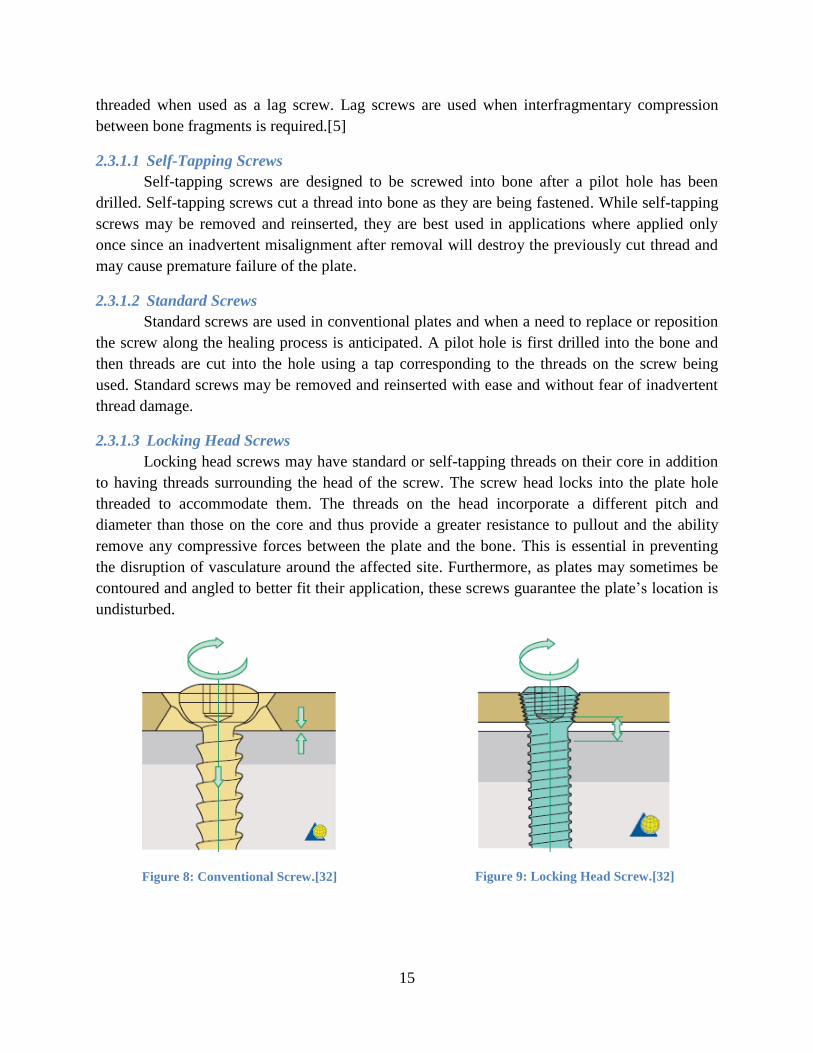
Figure 8: Conventional Screw.[32] ............................................................................................... 15
Figure 9: Locking Head Screw.[32].............................................................................................. 15
Figure 10: Dynamic Compression Plate ....................................................................................... 17
Figure 11: Low Contact Dynamic Compression Plate ................................................................. 17
Figure 12: Locking Compression Plate......................................................................................... 18
Figure 13: String of Pearls Plate. .................................................................................................. 19
Figure 14: Fixin Plate.................................................................................................................... 19
Figure 15: Advanced Locking Plate System #10 .......................................................................... 20
Figure 16: Advanced Locking Plate System #11 .......................................................................... 20
Figure 17: Eccentric Drill Guide (Left). Universal Drill guide (Right). ....................................... 22
Figure 18: Screw Securing Orders "A" and "B". .......................................................................... 22
Figure 19: Bone Loading. (a) Axial tension/compression. (b) Bending. (c) Torsion. (d) Shear. . 25
Figure 20: Axial and Bending Load Distribution for Conventional Plating Systems.[5] ............. 25
Figure 21: Axial and Bending Load Distribution for Locked Plating Systems.[5] ...................... 25
Figure 22: Torsion Load Distribution for Conventional Plating Systems. Adapted from [47]. ... 26
Figure 23: Torsion Load Distribution for Locked Plating Systems. Adapted from [47] .............. 26
Figure 24: Bone Model Cross-Section. ......................................................................................... 28
Figure 25: Drilling Guide and Spacer. .......................................................................................... 30
Figure 26: Centering Jig................................................................................................................ 30
Figure 27: Fixin Screw Deflection. ............................................................................................... 31
Figure 28: Properly Installed Four-Point Bending Test Sample. .................................................. 32
Figure 29: Anvil Span Measurement Locations. Adapted from ASTM F382.[7] ........................ 33
Figure 30: Sample Load-Displacement Curve. ............................................................................. 33
Figure 31: Complete Torsion Bone Model Segment (a) Front View (b) Top View..................... 35
Figure 32: Initial Torsion Test Setup. ........................................................................................... 36
Figure 33: Positive Cycle Data for ALPS11 Cycled at 2Hz. ........................................................ 37
Figure 34: Assembled Bone Segment End. .................................................................................. 37
Figure 35: Sample Plating System run-out and Failure Summary. .............................................. 39
Figure 36: Sample Probability Plot. .............................................................................................. 39
Figure 37: Four-point bending plate deformation. From left to right: DCP, LCP, SS LC-DCP,
Ti LC-DCP, ALPS11, ALPS10, Fixin, and SOP. ....................................................... 47

vii
Figure 38: Fixin Bone Model Fracture and Plate Deformation at Plate/Bone Model Interface. .. 48
Figure 39: Fixin Bone Model Failure. .......................................................................................... 48
Figure 40: ALPS10 Progressive Failure. ...................................................................................... 50
Figure A.1: ALPS10, Sample 1 .................................................................................................... 59
Figure A.2: ALPS10, Sample 2 .................................................................................................... 59
Figure A.3: ALPS10, Sample 3 .................................................................................................... 60
Figure A.4: ALPS10, Sample 4 .................................................................................................... 60
Figure A.5: ALPS11, Sample 1 .................................................................................................... 61
Figure A.6: ALPS11, Sample 2 .................................................................................................... 61
Figure A.7: ALPS11, Sample 3 .................................................................................................... 62
Figure A.8: ALPS11, Sample 4 .................................................................................................... 62
Figure A.9: DCP, Sample 1 .......................................................................................................... 63
Figure A.10: DCP, Sample 2 ........................................................................................................ 63
Figure A.11: DCP, Sample 3 ........................................................................................................ 64
Figure A.12: DCP, Sample 4 ........................................................................................................ 64
Figure A.13: Fixin, Sample 1 ........................................................................................................ 65
Figure A.14: Fixin, Sample 2 ........................................................................................................ 65
Figure A.15: Fixin, Sample 3 ........................................................................................................ 66
Figure A.16: Fixin, Sample 4 ........................................................................................................ 66
Figure A.17: SS LC-DCP, Sample 1 ............................................................................................ 67
Figure A.18: SS LC-DCP, Sample 2 ............................................................................................ 67
Figure A.19: SS LC-DCP, Sample 3 ............................................................................................ 68
Figure A.20: SS LC-DCP, Sample 4 ............................................................................................ 68
Figure A.21: Ti LC-DCP, Sample 1 ............................................................................................. 69
Figure A.22: Ti LC-DCP, Sample 2 ............................................................................................. 69
Figure A.23: Ti LC-DCP, Sample 3 ............................................................................................. 70
Figure A.24: Ti LC-DCP, Sample 4 ............................................................................................. 70
Figure A.25: LCP, Sample 1 ......................................................................................................... 71
Figure A.26: LCP, Sample 2 ......................................................................................................... 71
Figure A.27: LCP, Sample 3 ......................................................................................................... 72
Figure A.28: LCP, Sample 4 ......................................................................................................... 72
Figure A.29: SOP, Sample 1 ......................................................................................................... 73
Figure A.30: SOP, Sample 2 ......................................................................................................... 73
Figure A.31: SOP, Sample 3 ......................................................................................................... 74
Figure A.32: SOP, Sample 4 ......................................................................................................... 74
Figure D.1: ALPS10 Staircase Data Summary ............................................................................. 79
Figure D.2: ALPS11 Staircase Data Summary ............................................................................. 79
Figure D.3: DCP Staircase Data Summary ................................................................................... 80
Figure D.4: Fixin Staircase Data Summary .................................................................................. 80
Figure D.5: LCP Staircase Data Summary ................................................................................... 81

viii
Figure D.6: LC-DCP Staircase Data Summary ............................................................................ 81
Figure D.7: SOP Staircase Data Summary ................................................................................... 82
Figure F.1: ALPS10 Probability Plot, Percentage of Failure Torque. .......................................... 85
Figure F.2: ALPS10 Probability Plot, Absolute Torque Value. ................................................... 85
Figure F.3: ALPS11 Probability Plot, Percentage of Failure Torque. .......................................... 86
Figure F.4: ALPS11 Probability Plot, Absolute Torque Value. ................................................... 86
Figure F.5: Probability Plot, Percentage of Failure Torque. ......................................................... 87
Figure F.6: DCP Probability Plot, Absolute Torque Value. ......................................................... 87
Figure F.7: Fixin Probability Plot, Percentage of Failure Torque. ............................................... 88
Figure F.8: Fixin Probability Plot, Absolute Torque Value.......................................................... 88
Figure F.9: LCP Probability Plot, Percentage of Failure Torque. ................................................ 89
Figure F.10: LCP Probability Plot, Absolute Torque Value. ........................................................ 89
Figure F.11: LC-DCP Probability Plot, Percentage of Failure Torque......................................... 90
Figure F.12: LC-DCP Probability Plot, Absolute Torque Value. ................................................. 90
Figure F.13: SOP Probability Plot, Percentage of Failure Torque. .............................................. 91
Figure F.14: SOP Probability Plot, Absolute Torque Value. ........................................................ 91

ix
Table of Figures
Table 1: Greyhound and Pit-bull Long Bone Mechanical Properties.[8] ....................................... 5
Table 2: UTS and Max Elongation of tissues throughout fracture healing.[5] ............................... 7
Table 3: Plate and screw system features. .................................................................................... 29
Table 4: Bone Segment Lengths ................................................................................................... 35
Table 5: Sample Dixon-Mood Variable Calculation. ................................................................... 41
Table 6: Four-Point Bending Mechanical Property Summary. .................................................... 42
Table 7: Four-Point Bending Tukey Analysis Summary .............................................................. 43
Table 8: Plating System Torque Values........................................................................................ 44
Table 9: Plating System Failure Mode Occurrences. .................................................................... 44
Table 10: Mean Fatigue Strength Calculations. ............................................................................ 45
Table 11: Dixon-Mood and Svensson-Loren Standard Deviation Comparison. .......................... 46
Table B.1: Proof Load Calculations.............................................................................................. 75
Table B.2: Bending Stiffness Calculations. .................................................................................. 75
Table B.3: Bending Structural Stiffness Calculations. ................................................................. 75
Table B.4: Bending Strength Calculations.................................................................................... 76
Table G.1: ALPS10 Dixon-Mood Calculations. ........................................................................... 92
Table G.2: ALPS11 Dixon-Mood Calculations. ........................................................................... 92
Table G.3: DCP Dixon-Mood Calculations. ................................................................................. 92
Table G.4: Fixin Dixon-Mood Calculations. ................................................................................ 92
Table G.5: LCP Dixon-Mood Calculations. ................................................................................. 92
Table G.6: LC-DCP Dixon-Mood Calculations. .......................................................................... 93
Table G.7: SOP Dixon-Mood Calculations. ................................................................................. 93
1
1. Introduction
The understanding of bone healing and principles of fracture fixation has greatly
developed over the past half century. Depending on the method of fixation, bone may heal in
unstable or stable modes. An unstable fracture begins healing spontaneously, forming a
protruding callus at the fracture site in the process. If a fracture is left to heal in this mode, it may
take between six and nine years to fully complete the healing process. Fracture healing under
stable fixation methods occurs without formation of callus, and reduces fracture healing times to
about eighteen months. As controlling the movement and exercise of a canine with a fractured
leg is difficult, stable fixation is preferred.
Medical devices for human use must meet numerous requirements and regulations set by
the Food and Drug Administration (FDA) to ensure their safety and effectiveness. While the
FDA recommends that manufacturers of veterinary devices conduct tests to ensure their safety
and effectiveness, there are no regulations governing their approval for use. Consequently, very
few studies have been conducted calculating different mechanical properties of fracture fixation
systems and assessing their similarities and differences. Studies researched varied in their testing
methods as analyzed fixation devices were limited in addition to a restricted number of studies
utilizing in vivo loading considerations. This limitation prevents the surgeon from determining
the preferred fixation mode.[1-3]
Forces must be applied to bone to facilitate healing. When fixators are used to stabilize
bone fracture fragments, it is important for the stiffness of those fixators to be similar to that of
bone. As stated by Wolff’s law, bone undergoes many adaptations throughout its life to adapt to
its mechanical environment. As such, if fixators absorb a majority of the load placed on the bone,
stress shielding will effectively cause the fragment ends to resorb. This can lead to delayed
union, nonunion, or lack of bone growth.
Fixation plates are used for the stabilization of fractures in animals and humans. Using
the canine femur as a model, there exist numerous principal plate systems, of which the most
prominent were evaluated. Each of these systems contains a plate to span the fracture gap and
corresponding screws to affix the plate to the bone. These systems vary in their plate dimensions
and geometry, screw type, screw hole quantity, healing mode of plate application – ultimately
affecting the effectiveness, stiffness, and longevity of the system when placed under acute and
cyclic loads. Using a synthetic bone model and set fracture gap, the plating systems were
subjected to experiments to determine their bending strength under acute four-point bending
loads and their fatigue strength under cyclic torsion loads, as excess loading in these modes are
typically responsible for bone fracture.

2
2. Background
Bones are comprised of numerous tissues, vessels, and chemical structures and serve as a
rigid frame for the body’s tissues while also protecting internal organs from impact forces.[4]
More importantly, fracture or other damage should not occur from strain caused by repetitive
everyday activities. However, depending on an activity’s intensity level, duration, and repeated
loading, microscopic damage may be seen.[5] While osteoclasts and osteoblasts work together to
repair and maintain the structural integrity of bone, any damage occurring faster than the rate of
repair will experience fracture. Bone fracture may heal through different methods depending on
the damage level or fixation stability. Spontaneous healing occurs in fractures that are not fixated
in a stable manner, while primary healing occurs in rigidly fixed fractures.[5] As this study
focuses on femoral fracture fixator evaluation, the main fracture types associated with the
diaphysis of the femur are transverse, oblique, and comminuted. Numerous fixation methods
including intramedullary nails, pins, lag screws, and plating systems can be used to fixate these
fractures, in addition to allowing them to heal spontaneously without fracture stabilization.
2.1 Bone
The structure of bone can be broken down into multiple levels. While osseous tissue
dominates the makeup of bone, numerous structures exist on microscopic and chemical levels.
Epiphysis refers to the proximal and distal ends of bone while diaphysis refers to the main shaft.
A majority of the epiphysis is comprised of cancellous bone while the majority of the diaphysis
is comprised of cortical bone.
2.1.1 Bone Anatomy
Mammalian bone, including that of humans and canines, is a composite material
consisting of an organic matrix and inorganic hydroxyapatite. The wet weight of bone is derived
10-20% from water, 45-60% from hydroxyapatite (HA), and 30-35% from organic substances.
The organic composition can be further broken down to 90-95% collagen, 1%
glycosaminoglycans, and 5% other proteins.[6]
There are four levels associated with the structure of bone. Fundamentally, HA crystals are
ingrained between the ends of adjacent collagen fibrils. When separate, HA and collagen do not
possess high mechanical properties, but their combined form yields a composite with excellent
mechanical properties[6]. Generally, bone is more ductile than HA and is able absorb more
energy before failure and bear higher loads as it is more rigid than collagen. On the second level,
lamellae form from the combined collagen-HA fibrils and have specific orientations which
define the strength limits in their primary loading direction. This arrangement of lamellae is seen
on the third level. A tubular Haversian osteon is one functional unit of bone, produced from the
circular and concentric lamellae structure and possesses its maximum strength along the long
axis.[5] This is seen in Figure 1.
3
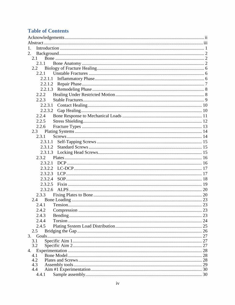
Figure 1: Structure of an Osteon[5]
The macroscopic structure of bone is observed on the fourth level of bone organization.
At this level, the main factors determining bone’s strength are its density and trabecular
orientation. There are two main bone structure types: cortical and cancellous. Cortical, or
compact, bone is found mainly in the diaphysis of long bones and the exterior shell of other bone
types. Compact bone consists of Haversian osteon systems and interstitial bone regions. Osteons
are typically oriented in the longitudinal direction of long bones and are typically 200µm in
diameter and 10-20mm long. They are further composed of concentric lamellae 3-9 µm thick.[6]
Haversian canals run through the center of osteons and allow blood vessels to deliver nutrients to
osteocytes (bone cells). Biomechanically, cortical bone can be characterized as being semi-
brittle, viscoelastic, and its strength is orientation dependent. Figure 2 shows the microscopic
anatomy of compact bone.
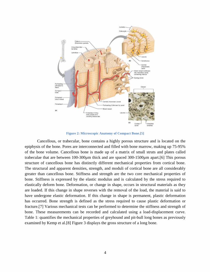
4
Figure 2: Microscopic Anatomy of Compact Bone.[5]
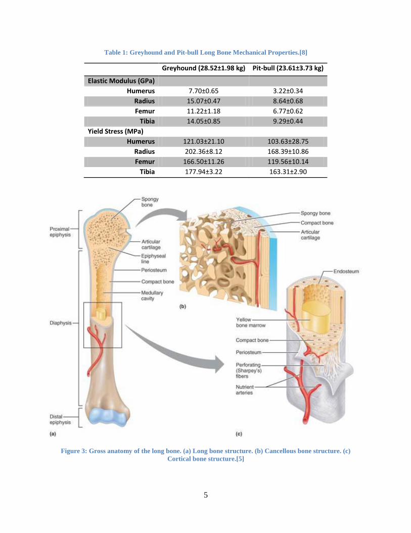
Cancellous, or trabecular, bone contains a highly porous structure and is located on the
epiphysis of the bone. Pores are interconnected and filled with bone marrow, making up 75-95%
of the bone volume. Cancellous bone is made up of a matrix of small struts and plates called
trabeculae that are between 100-300µm thick and are spaced 300-1500µm apart.[6] This porous
structure of cancellous bone has distinctly different mechanical properties from cortical bone.
The structural and apparent densities, strength, and moduli of cortical bone are all considerably
greater than cancellous bone. Stiffness and strength are the two core mechanical properties of
bone. Stiffness is expressed by the elastic modulus and is calculated by the stress required to
elastically deform bone. Deformation, or change in shape, occurs in structural materials as they
are loaded. If this change in shape reverses with the removal of the load, the material is said to
have undergone elastic deformation. If this change in shape is permanent, plastic deformation
has occurred. Bone strength is defined as the stress required to cause plastic deformation or
fracture.[7] Various mechanical tests can be performed to determine the stiffness and strength of
bone. These measurements can be recorded and calculated using a load-displacement curve.
Table 1: quantifies the mechanical properties of greyhound and pit-bull long bones as previously
examined by Kemp et al.[8] Figure 3 displays the gross structure of a long bone.
5
Table 1: Greyhound and Pit-bull Long Bone Mechanical Properties.[8]
Greyhound (28.52±1.98 kg) Pit-bull (23.61±3.73 kg)
Elastic Modulus (GPa)
Humerus 7.70±0.65 3.22±0.34
Radius 15.07±0.47 8.64±0.68
Femur 11.22±1.18 6.77±0.62
Tibia 14.05±0.85 9.29±0.44
Yield Stress (MPa)
Humerus 121.03±21.10 103.63±28.75
Radius 202.36±8.12 168.39±10.86
Femur 166.50±11.26 119.56±10.14
Tibia 177.94±3.22 163.31±2.90
Figure 3: Gross anatomy of the long bone. (a) Long bone structure. (b) Cancellous bone structure. (c)
Cortical bone structure.[5]
6
2.2 Biology of Fracture Healing
When bone experiences a load exceeding its ultimate tensile strength, fracture occurs.
Fracture is defined as a breach in continuity of bone, either on a macroscopic or microscopic
level. Fractures may heal via indirect or direct healing, depending on their relative stability.
2.2.1 Unstable Fractures
Unstable fractures heal via indirect healing, which is characterized by the formation of
callus as a process intermediate before modeling into hard bone.[5] This is also the mode of
healing for nonoperative fracture treatment, unstable internal and external fixation, along with
the plate osteosynthesis of highly comminuted fractures.[9, 10] The amount of callus produced is
inversely proportional to the stability of the fraction, as a less stable fracture results in increased
callus formation, and vice versa.[11] This is dictated by interfragmentary strain.
Interfragmentary strain is the deformation which occurs at a fracture’s bone fragment
interface. This is a major influence in the progression of fracture healing and is calculated by
dividing the displacement of the fracture gap by the initial gap width. Bone and callus formation
cannot occur with an interfragmentary strain greater than two percent. To overcome high strain,
muscles surrounding the bone first contract to begin resorption of the fragment ends. At strains
between two and ten percent, a fibrocartilage forms and between ten and one-hundred percent a
granulation tissue forms.[12] Once the tissues surrounding the fragment provide an
interfragmentary strain below two-percent, callus formation may begin.[5] The timeline of
unstable fracture healing is divided into three overlapping phases: inflammatory, repair, and
remodeling.
2.2.1.1 Inflammatory Phase
Once the integrity of bone and its surrounding tissues are disrupted, the inflammatory
phase begins and continues until the initiation of cartilage or bone formation. This typically lasts
three to four days depending on the level of damage and magnitude of force causing the bone
disruption.[5] Within hours after bone disruption, an extraosseous blood supply emerges from
the surrounding tissues to begin the revascularization of the hypoxic fracture site. This forms a
fibrin rich clot and initiates spontaneous healing. Growing evidence suggests that hematoma
fosters the repair phase by releasing growth factors to stimulate angiogenesis and bone
formation.[5] Vasoactive substances are released by mast cells and are believed to contribute to
new vessel formation.[13] Macrophages also play a role in fracture repair as they release
fibroblast growth factor (FGF), initiating fibroplasia both in soft tissues and in bone. As
vasculature is reconstructed, internal, or medullary, blood flow resumes and the extraosseous
blood supply diminishes. Mesenchymal stem cells (MSCs) from the cambium layer of the
periosteum, endosteum, bone marrow, and adjacent soft tissues proliferate during this phase.[9]
Unless infection, excessive motion, or extensive necrosis of the soft tissue is noted, the
hematoma will resorb by the end of the first week after bone disruption. The end of this phase is
marked by a decreased observation in pain or swelling.

7
2.2.1.2 Repair Phase
During the repair phase, hematoma is transformed into granulation tissue with assistance
from capillary ingrowth, mononuclear cells, and fibroblasts. While interfragmentary strain
remains high in this phase, the sustained formation of granulation tissue is explained by its
ability to stretch to twice its length. The first observation of mechanical strength in the disrupted
bone is observed during this phase as the formed granulation tissue has a tensile strength of 0.1
N/m2. Granulation tissue helps reduce interfragmentary strain at the fracture site and in turn
initiates cartilage formation.[5, 11] The tissue matures predominantly into Type I collagen fibers
that have an ultimate tensile strength of 1-60 N/m2 and can resist elongation to a maximum of
17%.[5] As the fibers mature, they organize into a diagonal pattern to allow for optimized
elongation ability. Many elements including low oxygen tension, poor vascularity, growth
factors, and interfragmentary strain influence the ability of the collagen fibers to develop into a
cartilaginous callus. Proliferated MSCs present from the inflammatory phase are orchestrated by
TGF- and morphogenic proteins (BMPs) to differentiate into chondrocytes. This differentiation
is essential to the maturation of collagenous fibers at the fracture gap into internal and external
cartilaginous “soft callus” matrices, which are facilitated by angiogenesis and an intact
periosteum. In well-vascularized unstable fractures, a bulging external callus is also found,
increasing the injured bone’s resistance to bending. An increase in proteoglycan concentrations
in the fibrocartilage is observed, contributing to increased stiffness at the interfragmentary gap.
This callus resists compression, but has a similar ultimate tensile strength and elongation before
rupture as fibrous tissue (4-19 N/m2, 10-12.8%). Once interfragmentary strain reduces to below
ten percent, this cartilaginous matrix may mineralize, maturing into “hard callus” by
endochondral ossification.[9, 11] In this process, chondrocytes calcify and degenerate, facilitate
angiogenesis, and allow osteoblasts to lay down woven bone on the collagen framework left by
the chondrocytes.
The length of time necessary to achieve union depends on the fracture configuration and
location, the status of adjacent soft tissues, in addition to the patient’s statistics. While bone
union is achieved at the end of the repair phase, its existing structure at the fracture site does not
resemble that of the original bone. At the end of the repair phase, however, enough strength and
rigidity has been regained to allow a canine to begin low impact exercise. Table 2 describes the
ultimate tensile strength and maximum elongation of tissues formed throughout the fracture
healing process.
Table 2: UTS and Max Elongation of tissues throughout fracture healing.[5]
UTS (N/m
2) Max Elongation
Granulation Tissue 0.1 200%
Collagen Fibers 1-60 17%
Early soft callus 4-19 10-12.8%
Bone 130 2%

8
2.2.1.3 Remodeling Phase
In the final phase of fracture repair, hard callus undergoes a morphological adaptation to
regain the optimal function and strength of intact bone. In humans, 6-9 years can pass until the
process completes, and represents 70% of the total healing time. During this phase, the woven
hard callus remodels into the required amount of lamellar bone and any excess callus is removed,
thereby restoring the medullary canal and bone shape.[11] Bone is arranged in areas
experiencing excess stress and removed from areas where there is too little, according to the
accepted theory known as Wolff’s Law which states that bone structure constantly adapts to the
mechanical loads to which it is subject.
Figure 4 shows the phases and time distribution required to spontaneously heal bone. As
previously described, the progression of soft to hard callus in spontaneous fracture healing is
dependent on the fracture site being supplied with sufficient blood in addition to consistent
increase in stability. Without these two factors, fibrous tissue will not advance to hard callus and
will lead to an atrophic nonunion. This is typically remedied with the addition of bone grafts or
removing the layer of both on the two apposed fracture ends to restart the healing process. If
proper vasculature exists without interfragmentary motion control, the fracture will progress into
a cartilaginous callus unable to stabilize the fragments and will further progress into hypertrophic
nonunion. This is typically remedied with the addition of rigid fixation. When canine bone
undergoes spontaneous bone repair, malunion is not uncommon.[5]
Figure 4: Phase Timeline of Spontaneous Healing.[5]
2.2.2 Healing Under Restricted Motion
Fractures controlled under restricted motion heal in a process intermediate to spontaneous
healing of uncontrolled fractures and healing after absolute stabilization. To limit motion at the

9
fracture gap and minimize the likelihood of malalignment, pins and nails are often implanted.
Healing of fractures under restricted motion begins with some resorption of the fragment ends.
Primitive implantation methods advised reaming the medullary canal prior to implanting nails,
thereby removing bone marrow and disrupting endosteal blood flow. This allowed for the largest
possible nail diameter to be implanted in the medullary canal. The initial stability of these
implants is attributed to the contact between the nail and the bone’s inner cortex, in addition to
the screws used to provide rotational stability. The process of reaming prior to implantation,
however, decreases the blood supply available at the fracture site by 70%.[14] Since research has
established that an appropriate blood supply is required for fracture healing, nailing methods and
implants have been modernized to minimize disruption. This includes making optional the
reaming of the medullary canal in addition to changes to implant geometry, which together have
demonstrated only a 30% reduction in blood supply at the fracture site. Unreaming nails,
however, do not offer the initial fixation stability of reaming nails. Some research has shown that
the increased blood supply associated with unreamed implants may not correspond to improved
healing times.[15] While the restricted motion from IM nailing demonstrates a significant
improvement over spontaneous healing, the ossification associated with healing under restricted
motion is only about 10% of that associated with plate or external fixator stabilization.[15]
Advocates of unreamed nailing believe reaming of the intramedullary canal is detrimental as the
endosteal blood flow will be disrupted and may potentially further damage the bone.[15, 16]
Though studies have debated the healing success of reamed versus undreamed intramedullary
nails, stable fixation remains the most effective form of fracture management as it facilitates
direct healing.
External fixators may also be used to restrict motion and are applied using closed
reduction techniques while further minimizing vasculature disruption and maintaining stability.
The amount of callus formed is minimal but can vary greatly depending on the configuration of
the fracture and the rigidity of the fixator frame applied.[5] Variation can occur if the implant is
not placed on the tension side of the bone, fracture reduction is not perfect, or if the implant lacks
rigidity. These factors are most relevant in fixation of comminuted fractures since fragment ends
are more difficult to align properly and mechanical stability greatly influences the course of
healing. While closed reduction external fracture fixators offer decreased callus formation, their
structure may not provide adequate stability due to the moment created by implant being offset
from the body. More importantly, a higher probability of infection exists as the implant must
pass through the patient’s dermis in multiple locations. Overall, while healing by restricted
motion may pose benefits to the healing process over spontaneous healing, increased stability
and lack of callus formation resulting from stable fracture fixation is optimal.
2.2.3 Stable Fractures
In 1949, Danis reported that a callus is not formed during bone healing when two bone
fragments are apposed under a rigid plate and axially compressed.[5] Application of rigid,
nongliding implants, such as compression plates and lag screws results in a stable bone fragment
10
interlocking connection. It was later confirmed by Schenk and Willenegger that healing under
these conditions was the result of direct osteonal proliferation.[5, 17] This repair mode, termed
“primary” or “direct” healing, refers to direct filling of the fracture site with bone, without the
formation of periosteal or endosteal callus. Rigid fixation and precise reduction suppress the
biological signals found through indirect healing methods which attract callus promoting
osteoprogenitor cells to the fracture site.
Interfragmentary compression induced by a plating system creates differences in the
biomechanical microenvironment within the fracture site and influences the progression of bone
development.[5] Contact and compression areas are bounded regions separated by areas where
fragments ends are separated by small gaps. A compression plate applied across a fracture site
will create two different healing zones. The cortex directly under the plate will experience
contact and compression characteristics triggered by the plating system. The far cortex will be
exposed to forces in tension and will be subject to gap healing. Both contact and gap healing are
mechanisms classified under direct fracture healing. Utilization of plating systems to facilitate
primary healing remains the method of choice when fracture healing is required.[5]
2.2.3.1 Contact Healing
Contact healing in stable fractures is observed when the defect between bone ends is
smaller than 0.01mm and the interfragmentary strain is less than 2%.[3, 5, 9, 12] Lamellar bone
is directly formed as a result of primary osteonal reconstruction and is oriented in the normal
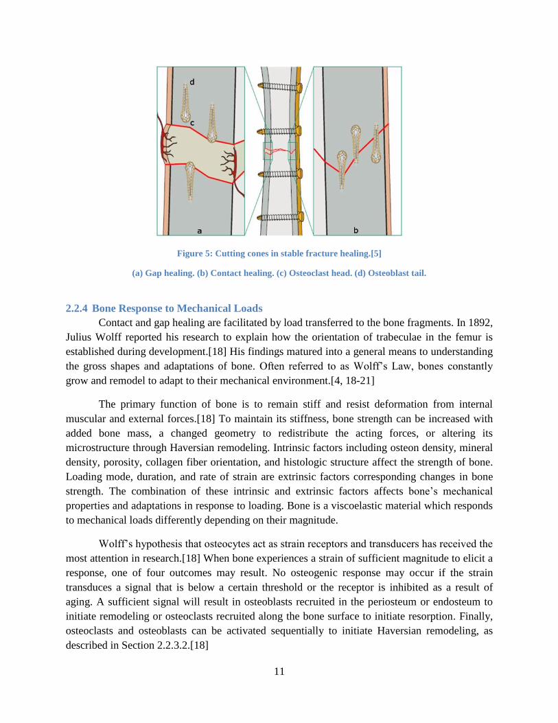
axial direction. Cutting cones are cells which form at the ends of the osteons closest to the
fracture site. These are seen in Figure 5, adapted from Rüedi et al.[5] Osteoclasts line the head of
the cutting cones while osteoblasts line the tail. This enables bony union and Haversian
remodeling to occur simultaneously.[5] Osteoclasts advance across the fracture site and create
longitudinally oriented cavities in which the osteoblastic ends deposit osteoids. Cutting cone
navigation has been reported across canine radial osteotomies under rigid fixation as early as
three weeks after surgery. Cutting cones travel across fragments at a rate of 50-100 µm/day and
become the “spot welds” which unite the fragment ends without the production of callus.[17]
The bone formed during remodeling will be visible on radiographs until bone density at the
fracture site reaches that of intact cortical bone.
2.2.3.2 Gap Healing
Direct healing at gaps between 800µm to 1mm occurs in a similar process to contact
healing, though bony union and Haversian remodeling remain separate, sequential steps.[9]
Healing starts with osteoblasts depositing layers of lamellar bone on both fracture surfaces,
perpendicular to the long axis, until the ends unite.[9] This area, however, remains weak due to
this bone orientation. Haversian remodeling initiates between three and eight weeks after surgery
when osteoclasts form on both fracture ends and create longitudinally oriented resorption
cavities. Longitudinally oriented lamellar bone is deposited into these cavities over time by the
osteoblast tail of the cutting cone so anatomical and mechanical integrity of the cortex may be
reestablished.[5]
11
Figure 5: Cutting cones in stable fracture healing.[5]
(a) Gap healing. (b) Contact healing. (c) Osteoclast head. (d) Osteoblast tail.
2.2.4 Bone Response to Mechanical Loads
Contact and gap healing are facilitated by load transferred to the bone fragments. In 1892,
Julius Wolff reported his research to explain how the orientation of trabeculae in the femur is
established during development.[18] His findings matured into a general means to understanding
the gross shapes and adaptations of bone. Often referred to as Wolff’s Law, bones constantly
grow and remodel to adapt to their mechanical environment.[4, 18-21]
The primary function of bone is to remain stiff and resist deformation from internal
muscular and external forces.[18] To maintain its stiffness, bone strength can be increased with
added bone mass, a changed geometry to redistribute the acting forces, or altering its
microstructure through Haversian remodeling. Intrinsic factors including osteon density, mineral
density, porosity, collagen fiber orientation, and histologic structure affect the strength of bone.
Loading mode, duration, and rate of strain are extrinsic factors corresponding changes in bone
strength. The combination of these intrinsic and extrinsic factors affects bone’s mechanical
properties and adaptations in response to loading. Bone is a viscoelastic material which responds
to mechanical loads differently depending on their magnitude.
Wolff’s hypothesis that osteocytes act as strain receptors and transducers has received the
most attention in research.[18] When bone experiences a strain of sufficient magnitude to elicit a
response, one of four outcomes may result. No osteogenic response may occur if the strain
transduces a signal that is below a certain threshold or the receptor is inhibited as a result of
aging. A sufficient signal will result in osteoblasts recruited in the periosteum or endosteum to
initiate remodeling or osteoclasts recruited along the bone surface to initiate resorption. Finally,
osteoclasts and osteoblasts can be activated sequentially to initiate Haversian remodeling, as
described in Section 2.2.3.2.[18]
12
Though the methods of sensing mechanical loads by bone cells are not well understood,
there are many indications that strain rate and magnitude are important stimuli effecting bone
response.[18, 21, 22] One of the hypotheses regarding the mechanism of mechanotransduction
which has received the most attention suggests that osteocytes are mechanosensors of shear
stresses.[23] Osteocytes have radiating canaliculi which communicate with other osteocytes
through transmitter proteins at gap junctions. Together, these osteocytes form a connected
cellular network surrounding the periosteal and endosteal membranes. These cells further
connect to osteoblasts lining the periosteum and endosteum which connect to preosteoblasts in
the membrane. Together, this network effectively creates a nervous system in the bone which
controls nutrient flow and initiates bone remodeling when activated.[18]
2.2.5 Stress Shielding
As described by Wolff’s law, mechanical loading of bone stimulates the initiation of
Haversian remodeling. One issue observed with the introduction of rigid fixation systems is bone
refracture after implant removal. Researchers have attributed this to bone atrophy as a result of
the fixation system bearing a majority of the load, and not the bone.[24] This phenomenon has
been termed stress shielding.
Stress shielding is a common occurrence with rigid fixation systems and results in a loss
of bone mass around the area where a plating system is applied.[12] The effects of this are
apparent when a system is comprised of two or more components, as these components typically
have different moduli of elasticity.[25, 26] An applied bone plating system, for example, creates
a system comprised of the fractured bone, fixation plate, and plate screws as the components,
which may all have different moduli of elasticity. When a load is placed on this system, the
stiffer component bears more of the load, thus “shielding” the other components.[25] Research
has suggested that fixation of fractured long bones with a plating system leads to osteoporosis
and the possibility of fatigue fracture after its removal.[25] Immature bone formation and
thinning of the cortical wall have been found at fracture sites shielded from loads by an apposed
rigid plate.[25] As a system’s material and geometry determine its stiffness, minimizing the
effects of stress shielding will require a system’s stiffness to be near that of bone. Preliminary
clinical research, however, has shown promise in the use of internal fixators for stable fracture
repair.[27]
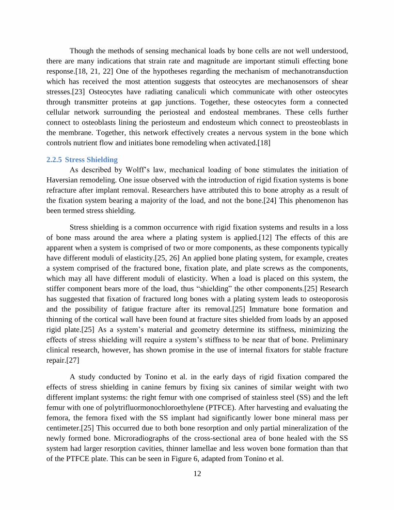
A study conducted by Tonino et al. in the early days of rigid fixation compared the
effects of stress shielding in canine femurs by fixing six canines of similar weight with two
different implant systems: the right femur with one comprised of stainless steel (SS) and the left
femur with one of polytrifluormonochloroethylene (PTFCE). After harvesting and evaluating the
femora, the femora fixed with the SS implant had significantly lower bone mineral mass per
centimeter.[25] This occurred due to both bone resorption and only partial mineralization of the
newly formed bone. Microradiographs of the cross-sectional area of bone healed with the SS
system had larger resorption cavities, thinner lamellae and less woven bone formation than that
of the PTFCE plate. This can be seen in Figure 6, adapted from Tonino et al.
13
Figure 6: Microradiographs of plated femora. (a) SS plate (b) PTFCE plate.[25]
Mechanical testing confirmed these observations impacted the bone’s strength as the
femora healed with SS plates required a 30% lower force to fracture, 22% lower bending
strength, and 20% lower modulus of elasticity than those healed with the PTFCE plate. The
observed histological and mechanical differences are entirely due to the plate material as both
systems had the same geometry and application area. It can therefore be concluded that the
material composition of the SS plating system played a role in the stress shielding effects
observed by the femora. Similar results have been reported by Diehl and Mittelmeier who
observed a loss of function in tibias healed with stainless steel plating systems. They found the
load required to fracture the bone to be one-third that of intact bone.[25] The effects of stress
shielding are further amplified with systems disrupting bone’s surrounding vasculature as this
prevents bone growth beneath the plate. Recent plating system developments have attempted to
address the issues surrounding stress shielding by changing plate material and geometry.
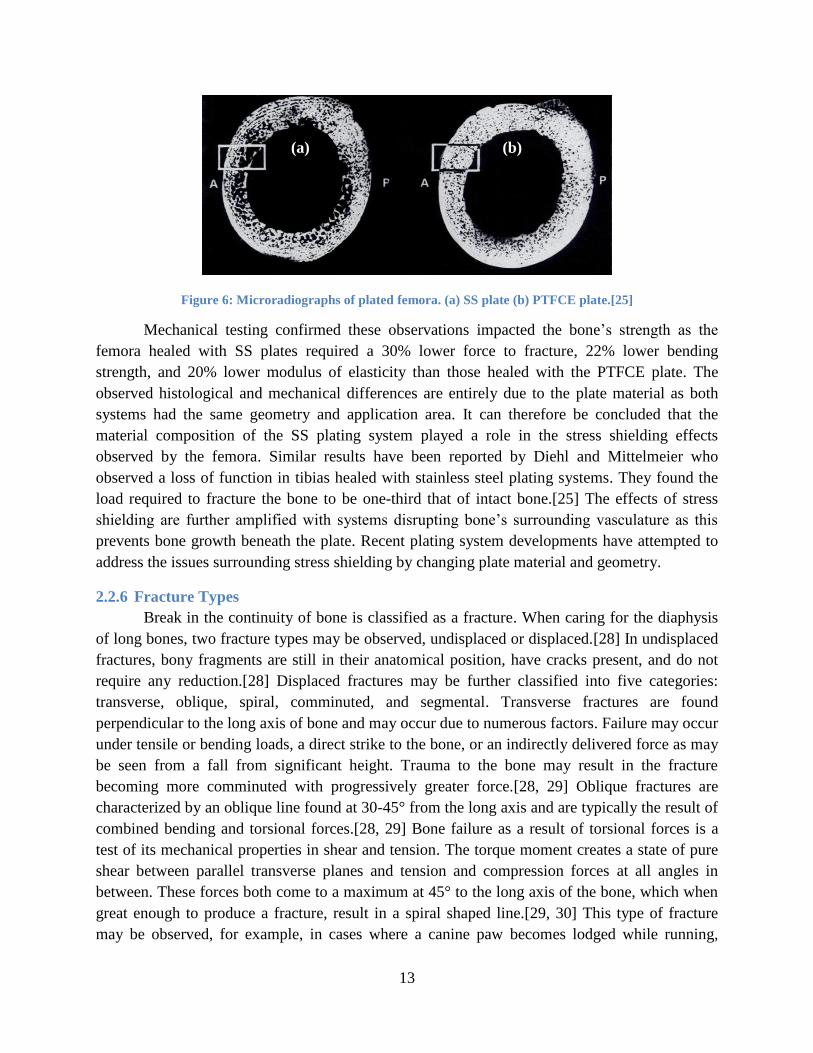
2.2.6 Fracture Types
Break in the continuity of bone is classified as a fracture. When caring for the diaphysis
of long bones, two fracture types may be observed, undisplaced or displaced.[28] In undisplaced
fractures, bony fragments are still in their anatomical position, have cracks present, and do not
require any reduction.[28] Displaced fractures may be further classified into five categories:
transverse, oblique, spiral, comminuted, and segmental. Transverse fractures are found
perpendicular to the long axis of bone and may occur due to numerous factors. Failure may occur
under tensile or bending loads, a direct strike to the bone, or an indirectly delivered force as may
be seen from a fall from significant height. Trauma to the bone may result in the fracture
becoming more comminuted with progressively greater force.[28, 29] Oblique fractures are
characterized by an oblique line found at 30-45° from the long axis and are typically the result of
combined bending and torsional forces.[28, 29] Bone failure as a result of torsional forces is a
test of its mechanical properties in shear and tension. The torque moment creates a state of pure
shear between parallel transverse planes and tension and compression forces at all angles in
between. These forces both come to a maximum at 45° to the long axis of the bone, which when
great enough to produce a fracture, result in a spiral shaped line.[29, 30] This type of fracture
may be observed, for example, in cases where a canine paw becomes lodged while running,
(a) (b)
14
indirectly distributing a torsional load to its long bones. A comminuted fracture is one where
more than two bone fragments exist, typically including small wedges and small fragments
which are nonreducible.[29, 31] Segmental fractures are a type of comminuted fracture where
the fragments are whole and large enough to be anatomically reconstructed.[5] Figure 7 depicts
these fracture types.
Figure 7: Fracture Types: (a) Transverse (b) Oblique (c) Spiral (d) Comminuted (e) Segmental.
2.3 Plating Systems
Screws and plates are used to achieve bony union of two or more fragment ends of a
fracture, whether surgery is performed with Open Reduction Internal Fixation (ORIF) or
Minimally Invasive Plate Osteosynthesis (MIPO) techniques. Depending on the type of fracture,
different plates may be used to facilitate the proper healing function. Plates may accommodate
conventional or locking screws. Multiple screw types may be used to attach a plate to bone.
These include cortical and cancellous screws with self-tapping or standard threads, and may have
locking heads. There are two plate types which can be applied: conventional and locking.
2.3.1 Screws
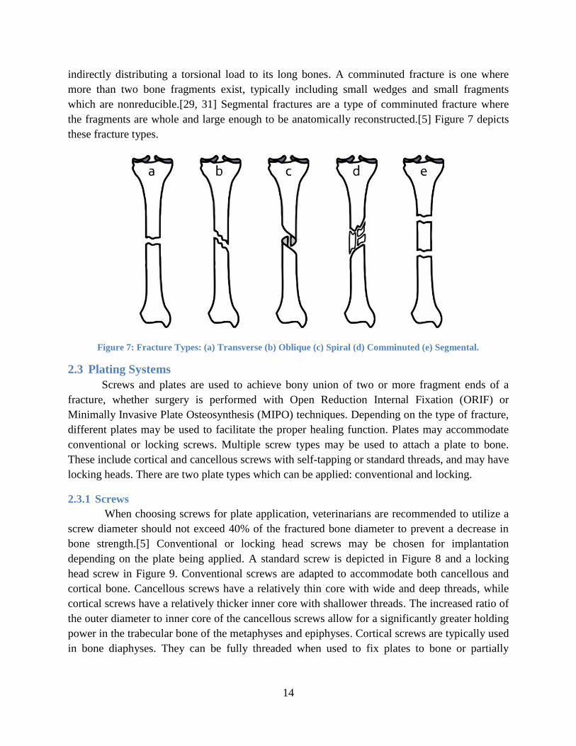
When choosing screws for plate application, veterinarians are recommended to utilize a
screw diameter should not exceed 40% of the fractured bone diameter to prevent a decrease in
bone strength.[5] Conventional or locking head screws may be chosen for implantation
depending on the plate being applied. A standard screw is depicted in Figure 8 and a locking
head screw in Figure 9. Conventional screws are adapted to accommodate both cancellous and
cortical bone. Cancellous screws have a relatively thin core with wide and deep threads, while
cortical screws have a relatively thicker inner core with shallower threads. The increased ratio of
the outer diameter to inner core of the cancellous screws allow for a significantly greater holding
power in the trabecular bone of the metaphyses and epiphyses. Cortical screws are typically used
in bone diaphyses. They can be fully threaded when used to fix plates to bone or partially
15
threaded when used as a lag screw. Lag screws are used when interfragmentary compression
between bone fragments is required.[5]
2.3.1.1 Self-Tapping Screws
Self-tapping screws are designed to be screwed into bone after a pilot hole has been
drilled. Self-tapping screws cut a thread into bone as they are being fastened. While self-tapping
screws may be removed and reinserted, they are best used in applications where applied only
once since an inadvertent misalignment after removal will destroy the previously cut thread and
may cause premature failure of the plate.
2.3.1.2 Standard Screws
Standard screws are used in conventional plates and when a need to replace or reposition
the screw along the healing process is anticipated. A pilot hole is first drilled into the bone and
then threads are cut into the hole using a tap corresponding to the threads on the screw being
used. Standard screws may be removed and reinserted with ease and without fear of inadvertent
thread damage.
2.3.1.3 Locking Head Screws
Locking head screws may have standard or self-tapping threads on their core in addition
to having threads surrounding the head of the screw. The screw head locks into the plate hole
threaded to accommodate them. The threads on the head incorporate a different pitch and
diameter than those on the core and thus provide a greater resistance to pullout and the ability
remove any compressive forces between the plate and the bone. This is essential in preventing
the disruption of vasculature around the affected site. Furthermore, as plates may sometimes be
contoured and angled to better fit their application, these screws guarantee the plate’s location is
undisturbed.
Figure 8: Conventional Screw.[32]
Figure 9: Locking Head Screw.[32]
16
2.3.2 Plates
Plates are designed to facilitate one or more of the following functions in fracture
fixation: compression, neutralization, bridging, or buttress. Compression plating generates axial
forces by use of a tensioning device or eccentrically loading screws. This mode is typically used
in simple transverse fractures and those with low obliquity. If a diaphyseal fracture is fixed with
a plate and screws to not produce any compressive axial forces, the system functions in a
neutralization mode.[33] In addition, as lag screws may be used to fix fragments in comminuted
fractures, a plate applied in neutralization mode protects the interfragmentary compression of the
fragments from any rotational, bending, or shears forces when loaded.[5] A plate functioning as
a buttress is applied to metaphyseal fractures to prevent the collapse of fragments when the
articular surface is exposed to compressive forces.[5] A plate functioning as a bridge is applied
when indirect reduction of bone is required, as in comminuted fractures. It functions as a splint to
maintain correct length of the bone and normal joint alignment when fixing the fragment ends as
it prevents axial deformity as a result of shear or bending forces.[5] Since the plate gets subjected
to full weight-bearing forces, it is important that the soft tissue surrounding the fragments
maintain their vascular supply as the success of indirect reduction is dependent on the formation
of the bridging callus.[5] In all plates depicted below, the top panel shows the top surface of the
plate, and the bottom panel shower the underside surface.
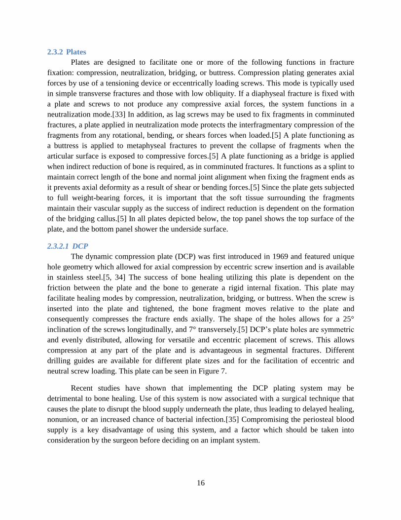
2.3.2.1 DCP
The dynamic compression plate (DCP) was first introduced in 1969 and featured unique
hole geometry which allowed for axial compression by eccentric screw insertion and is available
in stainless steel.[5, 34] The success of bone healing utilizing this plate is dependent on the
friction between the plate and the bone to generate a rigid internal fixation. This plate may
facilitate healing modes by compression, neutralization, bridging, or buttress. When the screw is
inserted into the plate and tightened, the bone fragment moves relative to the plate and
consequently compresses the fracture ends axially. The shape of the holes allows for a 25°
inclination of the screws longitudinally, and 7° transversely.[5] DCP’s plate holes are symmetric
and evenly distributed, allowing for versatile and eccentric placement of screws. This allows
compression at any part of the plate and is advantageous in segmental fractures. Different
drilling guides are available for different plate sizes and for the facilitation of eccentric and
neutral screw loading. This plate can be seen in Figure 7.
Recent studies have shown that implementing the DCP plating system may be
detrimental to bone healing. Use of this system is now associated with a surgical technique that
causes the plate to disrupt the blood supply underneath the plate, thus leading to delayed healing,
nonunion, or an increased chance of bacterial infection.[35] Compromising the periosteal blood
supply is a key disadvantage of using this system, and a factor which should be taken into
consideration by the surgeon before deciding on an implant system.
17
Figure 10: Dynamic Compression Plate
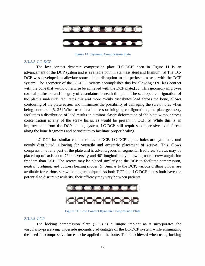
2.3.2.2 LC-DCP
The low contact dynamic compression plate (LC-DCP) seen in Figure 11 is an
advancement of the DCP system and is available both in stainless steel and titanium.[5] The LC-
DCP was developed to alleviate some of the disruption to the periosteum seen with the DCP
system. The geometry of the LC-DCP system accomplishes this by allowing 50% less contact
with the bone that would otherwise be achieved with the DCP plate.[35] This geometry improves
cortical perfusion and integrity of vasculature beneath the plate. The scalloped configuration of
the plate’s underside facilitates this and more evenly distributes load across the bone, allows
contouring of the plate easier, and minimizes the possibility of damaging the screw holes when
being contoured.[5, 35] When used in a buttress or bridging configurations, the plate geometry
facilitates a distribution of load results in a minor elastic deformation of the plate without stress
concentration at any of the screw holes, as would be present in DCP.[5] While this is an
improvement from the DCP plating system, LC-DCP still requires compressive axial forces
along the bone fragments and periosteum to facilitate proper healing.
LC-DCP has similar characteristics to DCP. LC-DCP’s plate holes are symmetric and
evenly distributed, allowing for versatile and eccentric placement of screws. This allows
compression at any part of the plate and is advantageous in segmental fractures. Screws may be
placed up off-axis up to 7° transversely and 40° longitudinally, allowing more screw angulation
freedom than DCP. The screws may be placed similarly to the DCP to facilitate compression,
neutral, bridging, and buttress healing modes.[5] Similar to the DCP, various drilling guides are
available for various screw loading techniques. As both DCP and LC-DCP plates both have the
potential to disrupt vascularity, their efficacy may vary between patients.
Figure 11: Low Contact Dynamic Compression Plate
2.3.2.3 LCP
The locking compression plate (LCP) is a unique implant as it incorporates the
vascularity-preserving underside geometric advantages of the LC-DCP system while eliminating
the need for compressive forces to be applied to the bone. This is achieved when using locking

18
head screws, though LCP is a combination hole plate which accommodates standard screws as
well.[36] One-half of each hole is designed to accommodate the standard DCP and LC-DCP
screws for fragment compression while the other half accommodates the locking head screws,
advantageous for angular stability and removal of compressive forces from the bone fragment
surfaces. As locking head screws have a larger core diameter, their use increases bending and
shear strengths while displacing the load across a larger area across the bone. Use of locking
head screws reduces the priority of perfectly contouring the plate due to the angular stability
produced.[36] This plate is illustrated in Figure 12.
In vitro biomechanical testing was conducted in a study by Aguila et al. comparing the
LC-DCP and LCP plates when fixed to 14 pairs of femora with a 20mm osteotomy gap. No
significant difference in structural stiffness of both plates was found in four-point bending. The
LC-DCP system was found to be significantly stiffer when tested in cyclic torsion.[36]
Figure 12: Locking Compression Plate
2.3.2.4 SOP
The string of pearls (SOP) plating system, illustrated in Figure 13, is a newer, stainless
steel locking plate system designed both for veterinary and human use. Though it is a locking
plate, it is secured using standard screws. Holes in the spherical “pearls” of the plate have threads
which correspond to those on the core of the screws. As the screw is secured to the plate, it
threads into the pearls and thus allows the screw to be properly torqued while removing any
compressive force acting on the bone. The SOP system is similar to that of the LCP as they both
locking plates which serve to minimize damage to the periosteal blood supply and minimize the
need for plate contouring to the bone. The SOP plate is comprised of cylindrical internodes
connecting the spheres, which have a greater moment of inertia over the DCP, LC-DCP, and
LCP plating systems due to their geometry. The internodes are 5mm in diameter while the
spheres are 8mm in diameter for all plate lengths. These cylindrical components allow the plate
to have up to six degrees of rotational freedom when contouring is necessary.[37] The design of
these components also prevents potential deformation of the screw holes when being contoured,
a drawback to the flat locking plate systems.
In a four-point bending study conducted by Ness, the SOP plating system attained a
higher bending stiffness, bending structural stiffness, and bending strength than the DCP
system.[37] Further testing was conducted comparing bent, twisted, and contoured SOP plates to
the untouched DCP plate. The results of these tests demonstrated that the twisted and contoured
SOP plate maintained higher strength and stiffness properties. No significant difference was

19
found between the mechanical properties of the bent SOP plate and the untouched DCP
plate.[37] Another study conducted by Ness evaluated the outcome of humeral fracture repair in
canines with a mean weight of 22.8 kg where two SOP systems were applied to the fracture.
Postoperative analysis of the thirteen canine humeri demonstrated satisfactory function of the
repaired limb in 12 of the 13 canines.[38] Additional surgery due to complications was recorded
in four canines, three of which demonstrated satisfactory function after healing. Refracture was
only evident in one canine. No screw loosening, backing out, or breakage was observed in the
115 SOP screws used for fracture fixation.[38] While the functional outcome following surgery
was excellent in most cases, no bone density analysis was performed analyzing the healed bone.
Figure 13: String of Pearls Plate.
2.3.2.5 Fixin
Fixin is a novel locking plate system which incorporates a bushing insert between the
screw-plate interfaces. It facilitates locking by creating a friction fit between the conical bushing
and screw head as the bushing threads screw into the plate and the screw threads into the
fractured bone. The bushing’s titanium make-up allows for easier removal of the implant as the
any concern of removal complications resulting from cold welding, cross threading, or damage
to the hexagonal screw recess previously reported with other locking plate systems.[39] This
combination of features allows the Fixin plating system to be angularly stable, simple to apply,
and easy to remove when necessary.
The Fixin plate is made of stainless steel and has threaded holes for the titanium bushing
inserts. The screws used in this plating system are typically stainless steel, self-tapping, and are
used in a locking mode. They have a larger core diameter to increase bending and shear strength
while also improving load distribution along the bone. The head of the screw incorporates a
conical surface matching that of the titanium insert, allowing stability through friction,
microwelding, and elastic deformation.[39] While no previous studies have been found
evaluating the stability and stiffness of this system, typical patients are canines and felines
weighing up to 10kg. This is illustrated in Figure 14.
Figure 14: Fixin Plate

20
2.3.2.6 ALPS
The Advanced Locking Plate System (ALPS) is a novel system incorporating a uniform
cross-sectional moment of inertia along the entire length of the plate due to its geometry where
the screw hole sections are wider than those connecting them.[40] The profile of this plate also
allows for improved periosteal blood flow in comparison to standard plates as there is minimal
contact with the bone.[40] The scalloped geometry and titanium makeup allow for increased
resistance to infection and deceased healing time as contact with the bone is decreased.[40] The
screw holes on the plate allow for standard screws to be placed in various angulations, or locking
head screws in fixed angulation. The locking mechanism of the hole functions by engaging the
threads on the screw shaft. As the screw reaches its last few threads by the screw head, the thread
diameter is reduced and the plate is pulled toward the bone when the locking mechanism is fully
engaged.[40] The conical interface between the screw heads and plate hole also allows both
screw types to be held in a stable position.
The manufacturer of this plating system, Kyon Pharma Inc., claims the strength of their
ALPS10 plating system is higher than that of the 3.5 DCP system.[41] In a study case report
written by Inauen et al., an ALPS5 plate was implanted into a two-year old feline to repair the
left hind limb lameness caused by a separation in an arthrodial joint of its foot. Five days post-
surgery, the owner reported no apparent lameness, and unrestricted activity was allowed.[40]
The surgeon had initially advised two weeks of cage rest followed by three weeks of restricted
activity. Clinical examination six weeks after surgery proved the feline was without lameness
and its left tarsus was stable and not swollen.[40] Furthermore, radiographs depicted uneventful
healing. As a result of this study, the ALPS system is shown to be effective in conditions where
standard compression plates may be applied for healing.[40] ALPS10 and ALPS11 are depicted
in Figure 15 and Figure 16.
Figure 15: Advanced Locking Plate System #10
Figure 16: Advanced Locking Plate System #11
2.3.3 Fixing Plates to Bone
In summary, conventional plates require compressive forces to be applied to the bone
fragments, require contouring to the bone, and may disrupt the bone’s surrounding vasculature
21
depending on the geometry of the plate’s underside. Locking plates do not require compressive
forces to be applied to the bone and also do not require exact contouring to the bone to facilitate
adequate healing and as a result of no compressive forces being applied to the bone, the bone’s
surrounding vasculature is preserved. However, due to their geometry and the method of
application, locking screws cannot be applied eccentrically in these plates to provide
compression at the fracture site.
When plating systems are required to heal bone fracture, Open Reduction Internal
Fixation (ORIF) or Minimally Invasive Plate Osteosynthesis (MIPO) techniques may be
employed to secure plates to bone. To allow proper alignment, ORIF utilizes direct reduction
techniques as the fracture site and surrounding tissues are exposed. This is typically achievable
with transverse, oblique, segmental, and comminuted fractures with one to three reducible
fragments.[5, 28] This treatment allows fragments to be perfectly aligned, but comes at the cost
of increase healing time due to the disruption of surrounding tissues. Plates fixed to these
fracture types will act in compression or neutralization modes. MIPO utilizes indirect reduction
techniques to align fracture fragments without exposing the fracture site or disrupting the
periosteum, thus maximizing the healing potential of the fracture site.[42] Reduction instruments
are inserted through skin incisions made near the fracture to align the fragments.[42] After
proper alignment, a plate is inserted through the incisions. Incisions are then made over the area
of the plate where screws are inserted. This is typically performed in undisplaced or highly
comminuted fractures.[42] Plates fixed to these fracture types will act in bridging or buttress.
Fractures reduced by direct reduction will be healed via direct healing.[5, 9] As anatomical
reconstruction is not possible in fractures reduced by indirect reduction techniques, these
fractures will heal via indirect healing.[5, 9] The correct plating system to stabilize a fracture is
dependent on the required fixation mode.
Plate size is typically dependent on the diameter of the fractured bone and the patient’s
weight, but is chosen at the surgeon’s discretion. Screw size is dependent on the requirements of
the plate being applied as the screw holes accommodate a certain size. After choosing the
appropriate plate and screw, a pilot hole is drilled for the chosen screw size using a drill bit and
drill sleeve for accurate alignment. While conventional plating systems allow the surgeon to
angulate the applied screws when inserted, studies have shown that insertion perpendicular to the
plate provides the highest resistance to pullout in normal bone and forty degrees off-axis the
lowest.[43] Different types of drill guides may be used to facilitate the intended function of the
plating system. These include a universal guide to center the drill in the plate hole for a Neutrally
applied screw for Neutralization, Bridging, and Buttress modes and an eccentric guide to offset
the drill to enable Compression mode.[5] Figure depicts the difference in screw application using
the two guides. When securing holes in an eccentrically drilled screw hole, the fragment ends of
the fracture being secured glide toward each other and apply a compressive force at the fracture
site. This is only possible in fractures that are transverse or minimally oblique, to ensure the
fragment ends do not slide when exposed to compressive axial forces along the bone.
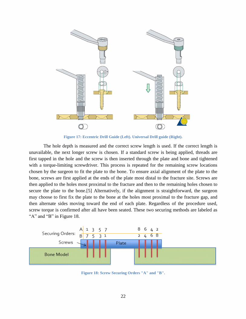
22
Figure 17: Eccentric Drill Guide (Left). Universal Drill guide (Right).
The hole depth is measured and the correct screw length is used. If the correct length is
unavailable, the next longer screw is chosen. If a standard screw is being applied, threads are
first tapped in the hole and the screw is then inserted through the plate and bone and tightened
with a torque-limiting screwdriver. This process is repeated for the remaining screw locations
chosen by the surgeon to fit the plate to the bone. To ensure axial alignment of the plate to the
bone, screws are first applied at the ends of the plate most distal to the fracture site. Screws are
then applied to the holes most proximal to the fracture and then to the remaining holes chosen to
secure the plate to the bone.[5] Alternatively, if the alignment is straightforward, the surgeon
may choose to first fix the plate to the bone at the holes most proximal to the fracture gap, and
then alternate sides moving toward the end of each plate. Regardless of the procedure used,
screw torque is confirmed after all have been seated. These two securing methods are labeled as
“A” and “B” in Figure 18.
Figure 18: Screw Securing Orders "A" and "B".

23
2.4 Bone Loading
There are four predominant mechanical testing methods used in the evaluation of bone
and plating systems: tension, compression, bending, and torsion. These sufficiently calculate
various mechanical properties of bone.
2.4.1 Tension
Tensile testing is a simple method of determining the mechanical properties of both
cortical and cancellous bone, though the specimen required is usually large. Prior to testing,
specimens are modified to form a dog bone-like shape to ensure a uniform strain in central
portion of the specimen. This test is not physiologically relevant as in vivo bone is not primarily
loaded in tension, though it may still be used to calculate Young’s modulus, ultimate strength,
and yield strength.[6, 30]
Only a limited number of studies evaluate the tensile properties of healing bone. In one
study, bone healing was investigated in an osteotomy of the diaphysis of the right sheep
metatarsal as a function of gap size and stability. Specimens containing callus were evaluated
nine weeks after surgery and were found to have a decreasing tensile strength with greater initial
interfragmentary gap.[44] For example, a one millimeter initial gap corresponded to a tensile
strength eight times lower than normal bone; a six millimeter gap resulted in a tensile strength 36
times lower than normal bone.
2.4.2 Compression
Compression testing is more commonly used to test cancellous bone as this is its most
physiologically relevant loading mode. Compression tests are advantageous as they require
smaller specimens compared to tensile tests, thus simplifying the mechanical testing. Most
importantly, compression testing more closely simulates in vivo loading conditions, especially in
vertebrae.[6]
Similar to tensile testing, few studies have reported compressive properties of healing
bone. The same study analyzing tensile properties of healing bone collected from a transverse
osteotomy in the midshaft of sheep metatarsal nine weeks after surgery reported compressive
testing results. Testing showed a great variation in mean indentation stiffness depending on
callus location, gap size, and stability.[44] A similar technique was used in a study using the
canine femoral osteotomy model. Specimens showed an increase in indentation stiffness from
2% to 25% from two to twelve weeks after surgery. The change in local stiffness over time also
correlated significantly to the increase in maximum torque and torsional stiffness.[45]
2.4.3 Bending
Bending tests can be performed either in three-point or four-point loading modes. Three-
point bending involves a simply supported beam with one load applied between the supporting
ends. Four-point bending applies two loads between the supporting ends. Bending tests allow
tensile stresses to be present on one side of the specimen while the other side experiences
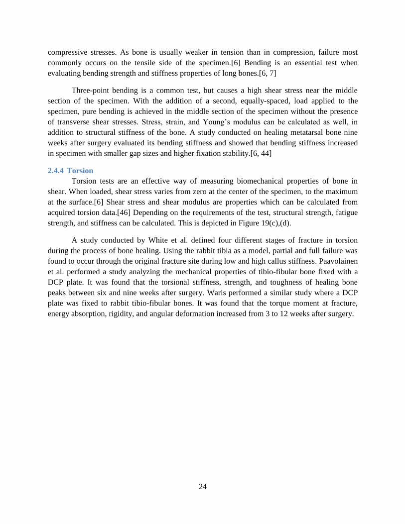
24
compressive stresses. As bone is usually weaker in tension than in compression, failure most
commonly occurs on the tensile side of the specimen.[6] Bending is an essential test when
evaluating bending strength and stiffness properties of long bones.[6, 7]
Three-point bending is a common test, but causes a high shear stress near the middle
section of the specimen. With the addition of a second, equally-spaced, load applied to the
specimen, pure bending is achieved in the middle section of the specimen without the presence
of transverse shear stresses. Stress, strain, and Young’s modulus can be calculated as well, in
addition to structural stiffness of the bone. A study conducted on healing metatarsal bone nine
weeks after surgery evaluated its bending stiffness and showed that bending stiffness increased
in specimen with smaller gap sizes and higher fixation stability.[6, 44]
2.4.4 Torsion
Torsion tests are an effective way of measuring biomechanical properties of bone in
shear. When loaded, shear stress varies from zero at the center of the specimen, to the maximum
at the surface.[6] Shear stress and shear modulus are properties which can be calculated from
acquired torsion data.[46] Depending on the requirements of the test, structural strength, fatigue
strength, and stiffness can be calculated. This is depicted in Figure 19(c),(d).
A study conducted by White et al. defined four different stages of fracture in torsion
during the process of bone healing. Using the rabbit tibia as a model, partial and full failure was
found to occur through the original fracture site during low and high callus stiffness. Paavolainen
et al. performed a study analyzing the mechanical properties of tibio-fibular bone fixed with a
DCP plate. It was found that the torsional stiffness, strength, and toughness of healing bone
peaks between six and nine weeks after surgery. Waris performed a similar study where a DCP
plate was fixed to rabbit tibio-fibular bones. It was found that the torque moment at fracture,
energy absorption, rigidity, and angular deformation increased from 3 to 12 weeks after surgery.
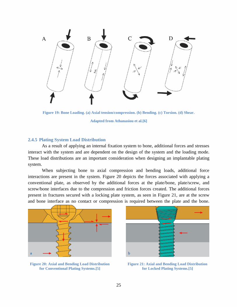
25
Figure 19: Bone Loading. (a) Axial tension/compression. (b) Bending. (c) Torsion. (d) Shear.
Adapted from Athanasiou et al.[6]
2.4.5 Plating System Load Distribution
As a result of applying an internal fixation system to bone, additional forces and stresses
interact with the system and are dependent on the design of the system and the loading mode.
These load distributions are an important consideration when designing an implantable plating
system.
When subjecting bone to axial compression and bending loads, additional force
interactions are present in the system. Figure 20 depicts the forces associated with applying a
conventional plate, as observed by the additional forces at the plate/bone, plate/screw, and
screw/bone interfaces due to the compression and friction forces created. The additional forces
present in fractures secured with a locking plate system, as seen in Figure 21, are at the screw
and bone interface as no contact or compression is required between the plate and the bone.
Figure 20: Axial and Bending Load Distribution
for Conventional Plating Systems.[5]
Figure 21: Axial and Bending Load Distribution
for Locked Plating Systems.[5]

26
Similarly, when subjecting the systems to torsional loads, Figure 22 and Figure 23 are
adapted from Gautier and Sommer and depict the additional force interactions in these
systems.[47]
Figure 22: Torsion Load Distribution for
Conventional Plating Systems. Adapted from [47].
Figure 23: Torsion Load Distribution for Locked
Plating Systems. Adapted from [47]
2.5 Bridging the Gap
Unlike medical devices for humans, no regulations exist in the Federal Food, Drug, and
Cosmetic Act under the FDA requiring evidence of the safety and effectiveness of veterinary
devices. Although several studies evaluate the functionality of one or two plating systems, no
research has been conducted evaluating the mechanical properties of each plating system in a
standardized fashion. Mechanical and clinical evaluation of plating system mechanics and bone
healing effectiveness will allow for a better understanding of system behavior in vivo and will
pronounce their benefits and faults. Evaluation of the eight most prevalent plating systems will
help veterinary surgeons better treat their canine patients with the optimal device for the
fractured bone by identifying plating characteristics which both support and inhibit fracture
healing.
27
3. Goals
The most prominent loading modes experienced by bone are bending and torsion. To
simulate this loading, two types of mechanical tests will be performed: four-point bending and
torsion. Mechanical tests will be conducted simulating a comminuted femoral fracture with a
plating system bridged across the gap. To diminish any variation with regard to bone geometry,
implant placement, implant shape, and gap size, a standardized model must be used. Through the
normal gait of canines, numerous forces act upon their bones translating primarily to a
combination of bending and torsional forces. Though the exact mode and intensity of loading is
not known, it is important to analyze the response of the plating systems to these loading
types.[48, 49] As described in ASTM F382, Standard Specification and Test Method for Metallic
Bone Plates, cyclic loading should allow for one million cycles to be placed on the plating
system without causing failure. Though it is important to analyze the cyclic loading properties in
each loading mode, testing machine limitations will allow us to only conduct cyclic loading in
torsion. The only previously conducted testing on these plating systems evaluated their single
cycle to failure properties in torsion. In this evaluation, we will determine the various mechanical
properties of these seven plating systems when simulating a comminuted fracture utilizing a
synthetic bone model.
3.1 Specific Aim 1
Evaluate the mechanical properties of eight plating
systems in single cycle to failure four-point bending.
Utilizing ASTM F382 as guidance, four-point bending tests will be conducted to evaluate
the mechanical properties of the various plating systems. The bending stiffnesses and strengths
will be calculated for each construct and compared to determine if any significant differences
exist. Furthermore, failure modes of each plating system will be noted. Due to limitations in the
equipment used for the acute four-point bending tests, cyclic loading will not be performed at
this time.
3.2 Specific Aim 2
Evaluate the fatigue strength of seven plating systems in cyclic torsional loading.
A previous evaluation has identified the acute failure torque in these systems.[50]
Utilizing the staircase method, samples will be cyclically torqued for evaluation. This will allow
us to ultimately determine the fatigue strength of each plating system utilizing probability plots
and Dixon-Mood analysis. Furthermore, failure modes of each plating system will be noted.

28
4. Experimentation
Acute failure properties were evaluated for eight plating systems using four-point
bending tests. Seven plating systems were evaluated for their fatigue strength using cyclic torsion
tests. While limited biomechanical data exist for a few of these systems, no data exist evaluating
them in a standardized manner. Samples were assembled in a fashion to simulate a comminuted
fracture utilizing a synthetic bone model as the fractured bone fragments and plating systems to
span the fracture gap.
4.1 Bone Model
To remove variability encountered with cadaveric bone, a synthetic bone model was used
in the mechanical testing. Short-fiber filled hollow epoxy (SFE) cylinders were previously
validated to simulate the mechanical properties of bone.[51] This study compared the elastic
modulus, maximum stress, and yield stress of synthetic bone models of various dimensions to
published pit-bull and greyhound femur, humerus, and tibia results.[8] Based on their results, the
bone model with a 20mm outer diameter and 3mm wall thickness best represented these
mechanical properties of native bone. The model used is depicted in Figure 24.
Figure 24: Bone Model Cross-Section.
4.2 Plates and Screws
Eight different plating systems were evaluated when used as a bridging plate and tested in
acute four-point bending, while only seven of these plating systems were evaluated in cyclic
torsion. While both SS and TI LC-DCP systems were evaluated in four-point bending, only the
SS LC-DCP system was evaluated in torsion due to limited sample quantities. These systems
included two conventional, four locking plates, and one combination standard/locking hole plate.
These plates were secured to the bone model with the appropriate screws corresponding to the
manufacturer’s specifications. These included standard and locking screws for both monocortical
and bicortical purchase. Table 3 below summarizes the properties of the plates and screws used.
It should be noted that only the locking holes were used in the combination hole LCP plate. In
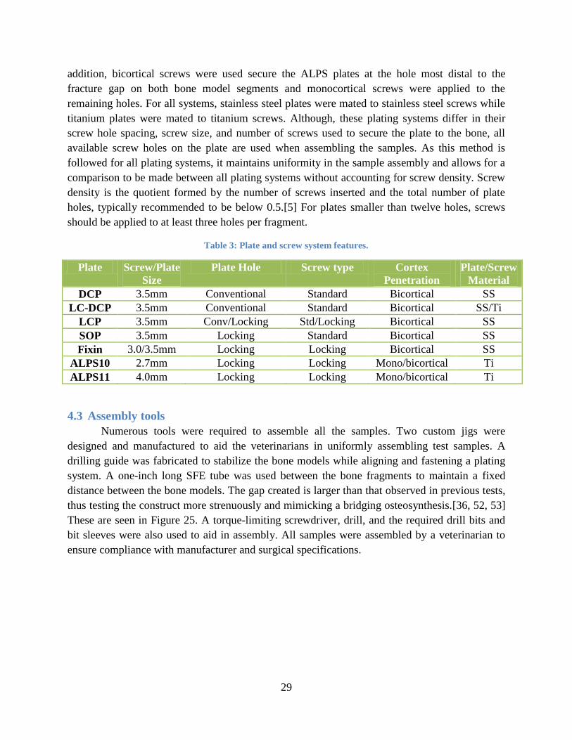
29
addition, bicortical screws were used secure the ALPS plates at the hole most distal to the
fracture gap on both bone model segments and monocortical screws were applied to the
remaining holes. For all systems, stainless steel plates were mated to stainless steel screws while
titanium plates were mated to titanium screws. Although, these plating systems differ in their
screw hole spacing, screw size, and number of screws used to secure the plate to the bone, all
available screw holes on the plate are used when assembling the samples. As this method is
followed for all plating systems, it maintains uniformity in the sample assembly and allows for a
comparison to be made between all plating systems without accounting for screw density. Screw
density is the quotient formed by the number of screws inserted and the total number of plate
holes, typically recommended to be below 0.5.[5] For plates smaller than twelve holes, screws
should be applied to at least three holes per fragment.
Table 3: Plate and screw system features.
Plate Screw/Plate
Size
Plate Hole Screw type Cortex
Penetration
Plate/Screw
Material
DCP 3.5mm Conventional Standard Bicortical SS
LC-DCP 3.5mm Conventional Standard Bicortical SS/Ti
LCP 3.5mm Conv/Locking Std/Locking Bicortical SS
SOP 3.5mm Locking Standard Bicortical SS
Fixin 3.0/3.5mm Locking Locking Bicortical SS
ALPS10 2.7mm Locking Locking Mono/bicortical Ti
ALPS11 4.0mm Locking Locking Mono/bicortical Ti
4.3 Assembly tools
Numerous tools were required to assemble all the samples. Two custom jigs were
designed and manufactured to aid the veterinarians in uniformly assembling test samples. A
drilling guide was fabricated to stabilize the bone models while aligning and fastening a plating
system. A one-inch long SFE tube was used between the bone fragments to maintain a fixed
distance between the bone models. The gap created is larger than that observed in previous tests,
thus testing the construct more strenuously and mimicking a bridging osteosynthesis.[36, 52, 53]
These are seen in Figure 25. A torque-limiting screwdriver, drill, and the required drill bits and
bit sleeves were also used to aid in assembly. All samples were assembled by a veterinarian to
ensure compliance with manufacturer and surgical specifications.
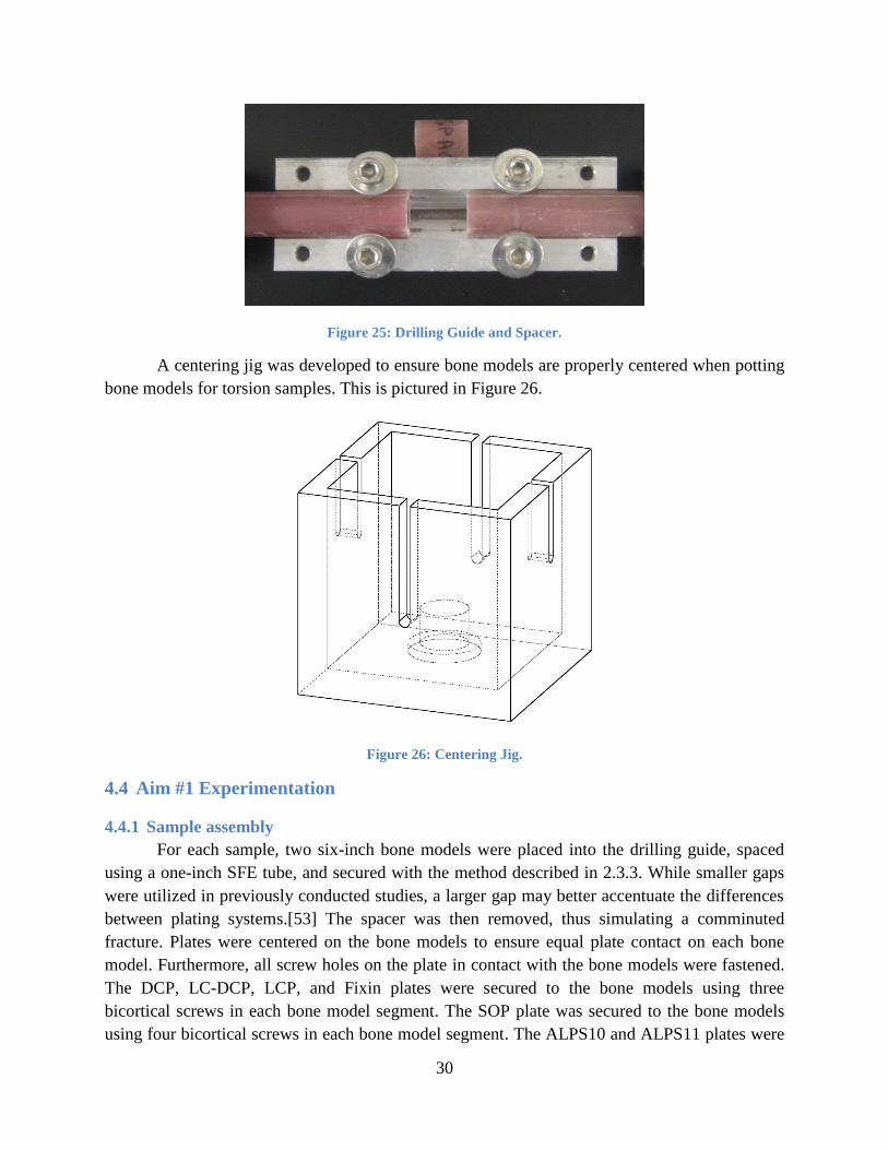
30
Figure 25: Drilling Guide and Spacer.
A centering jig was developed to ensure bone models are properly centered when potting
bone models for torsion samples. This is pictured in Figure 26.
Figure 26: Centering Jig.
4.4 Aim #1 Experimentation
4.4.1 Sample assembly
For each sample, two six-inch bone models were placed into the drilling guide, spaced
using a one-inch SFE tube, and secured with the method described in 2.3.3. While smaller gaps
were utilized in previously conducted studies, a larger gap may better accentuate the differences
between plating systems.[53] The spacer was then removed, thus simulating a comminuted
fracture. Plates were centered on the bone models to ensure equal plate contact on each bone
model. Furthermore, all screw holes on the plate in contact with the bone models were fastened.
The DCP, LC-DCP, LCP, and Fixin plates were secured to the bone models using three
bicortical screws in each bone model segment. The SOP plate was secured to the bone models
using four bicortical screws in each bone model segment. The ALPS10 and ALPS11 plates were
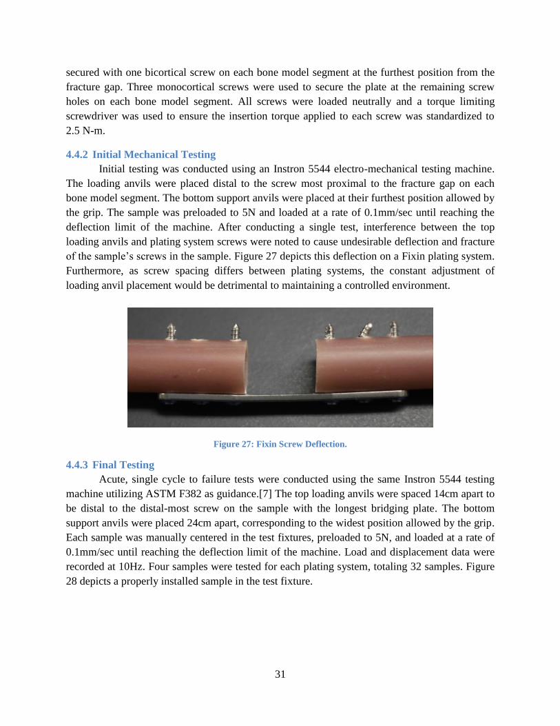
31
secured with one bicortical screw on each bone model segment at the furthest position from the
fracture gap. Three monocortical screws were used to secure the plate at the remaining screw
holes on each bone model segment. All screws were loaded neutrally and a torque limiting
screwdriver was used to ensure the insertion torque applied to each screw was standardized to
2.5 N-m.
4.4.2 Initial Mechanical Testing
Initial testing was conducted using an Instron 5544 electro-mechanical testing machine.
The loading anvils were placed distal to the screw most proximal to the fracture gap on each
bone model segment. The bottom support anvils were placed at their furthest position allowed by
the grip. The sample was preloaded to 5N and loaded at a rate of 0.1mm/sec until reaching the
deflection limit of the machine. After conducting a single test, interference between the top
loading anvils and plating system screws were noted to cause undesirable deflection and fracture
of the sample’s screws in the sample. Figure 27 depicts this deflection on a Fixin plating system.
Furthermore, as screw spacing differs between plating systems, the constant adjustment of
loading anvil placement would be detrimental to maintaining a controlled environment.
Figure 27: Fixin Screw Deflection.
4.4.3 Final Testing
Acute, single cycle to failure tests were conducted using the same Instron 5544 testing
machine utilizing ASTM F382 as guidance.[7] The top loading anvils were spaced 14cm apart to
be distal to the distal-most screw on the sample with the longest bridging plate. The bottom
support anvils were placed 24cm apart, corresponding to the widest position allowed by the grip.
Each sample was manually centered in the test fixtures, preloaded to 5N, and loaded at a rate of
0.1mm/sec until reaching the deflection limit of the machine. Load and displacement data were
recorded at 10Hz. Four samples were tested for each plating system, totaling 32 samples. Figure
28 depicts a properly installed sample in the test fixture.

32
Figure 28: Properly Installed Four-Point Bending Test Sample.
4.4.4 Aim #1 Results
After mechanically testing all the samples, the acquired data are evaluated to extrapolate
the bending stiffness, bending structural stiffness, and bending strength. Bending stiffness is
defined as the maximum slope of the linear-elastic portion of the load-displacement curve for
each sample. Bending strength is defined as the bending moment needed to generate a 0.2%
offset displacement in the sample. Finally, the bending structural stiffness is a normalized
effective bending stiffness taking the test setup configuration into consideration.
To calculate the various mechanical properties, anvil span measurements must first be
noted. Loading span, h, is defined as the distance between one bottom support anvil and the
nearest top loading anvil. Center span, a, is defined as the distance between the top loading
anvils. Both span measurements are used in their millimeter form. These values correspond to
50mm and 140mm, respectively, according to our test setup. Figure 29 is adapted from ASTM
F382 and depicts these measurement locations.[7]
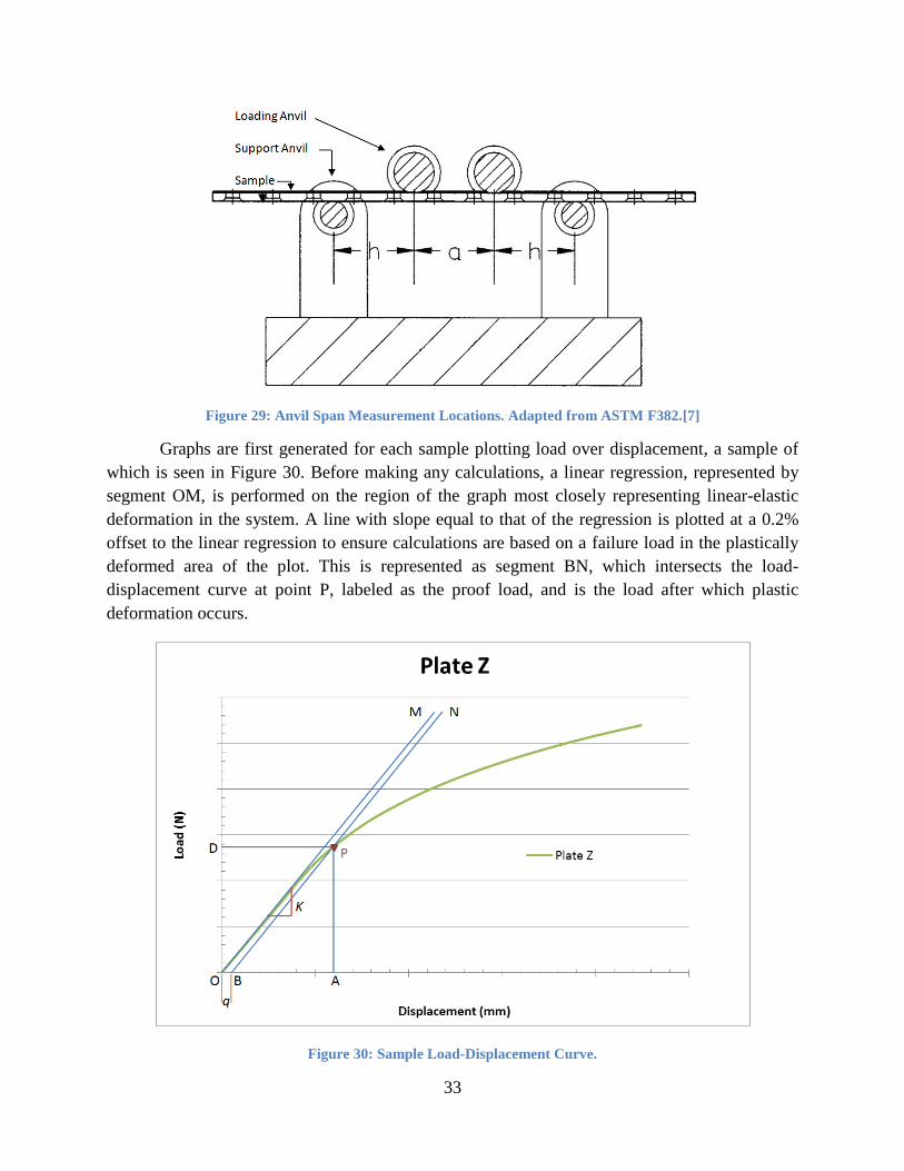
33
Figure 29: Anvil Span Measurement Locations. Adapted from ASTM F382.[7]
Graphs are first generated for each sample plotting load over displacement, a sample of
which is seen in Figure 30. Before making any calculations, a linear regression, represented by
segment OM, is performed on the region of the graph most closely representing linear-elastic
deformation in the system. A line with slope equal to that of the regression is plotted at a 0.2%
offset to the linear regression to ensure calculations are based on a failure load in the plastically
deformed area of the plot. This is represented as segment BN, which intersects the load-
displacement curve at point P, labeled as the proof load, and is the load after which plastic
deformation occurs.
Figure 30: Sample Load-Displacement Curve.
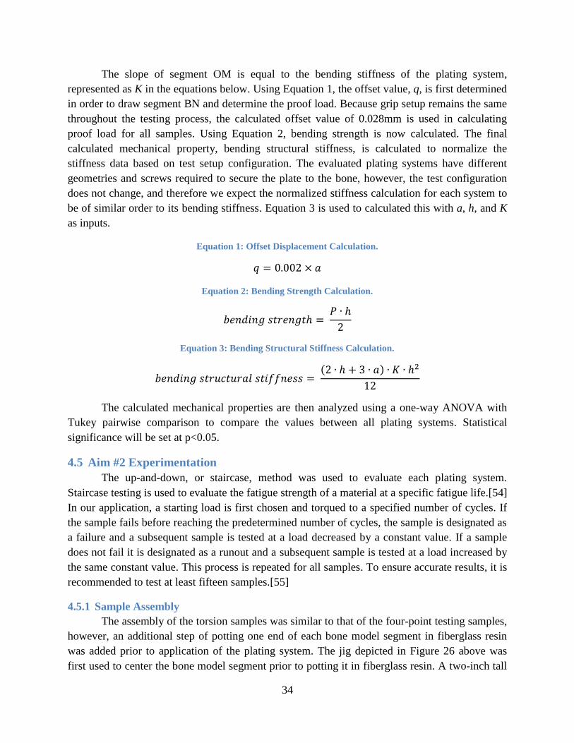
34
The slope of segment OM is equal to the bending stiffness of the plating system,
represented as K in the equations below. Using Equation 1, the offset value, q, is first determined
in order to draw segment BN and determine the proof load. Because grip setup remains the same
throughout the testing process, the calculated offset value of 0.028mm is used in calculating
proof load for all samples. Using Equation 2, bending strength is now calculated. The final
calculated mechanical property, bending structural stiffness, is calculated to normalize the
stiffness data based on test setup configuration. The evaluated plating systems have different
geometries and screws required to secure the plate to the bone, however, the test configuration
does not change, and therefore we expect the normalized stiffness calculation for each system to
be of similar order to its bending stiffness. Equation 3 is used to calculated this with a, h, and K
as inputs.
Equation 1: Offset Displacement Calculation.
Equation 2: Bending Strength Calculation.
Equation 3: Bending Structural Stiffness Calculation.
( )
The calculated mechanical properties are then analyzed using a one-way ANOVA with
Tukey pairwise comparison to compare the values between all plating systems. Statistical
significance will be set at p<0.05.
4.5 Aim #2 Experimentation
The up-and-down, or staircase, method was used to evaluate each plating system.
Staircase testing is used to evaluate the fatigue strength of a material at a specific fatigue life.[54]
In our application, a starting load is first chosen and torqued to a specified number of cycles. If
the sample fails before reaching the predetermined number of cycles, the sample is designated as
a failure and a subsequent sample is tested at a load decreased by a constant value. If a sample
does not fail it is designated as a runout and a subsequent sample is tested at a load increased by
the same constant value. This process is repeated for all samples. To ensure accurate results, it is
recommended to test at least fifteen samples.[55]
4.5.1 Sample Assembly
The assembly of the torsion samples was similar to that of the four-point testing samples,
however, an additional step of potting one end of each bone model segment in fiberglass resin
was added prior to application of the plating system. The jig depicted in Figure 26 above was
first used to center the bone model segment prior to potting it in fiberglass resin. A two-inch tall

35
and two-inch square PVC tube was inserted into the jig along with a bone model segment over
the centering nub. Two pins were then inserted perpendicularly through adjacent faces of the
PVC tube and bone model segment to keep the bone model segment centered upon removal from
the jig. When removed, this setup was placed on a sheet of cellophane wrap and the tube was
filled with resin to facilitate ultimate stability while testing. After the resin fully cured, the
respective plate was secured to the bone models with the method described in Section 4.4.1. The
length of the bone model segment varied between plates to allow a fixed distance between the
distal-most screw to the fracture gap and the top of the potting fiberglass resin. Table 4 below
lists the bone model segment lengths for all plating systems and Figure 31 depicts multiple views
of a complete bone model segment.
Table 4: Bone Segment Lengths
Plating System Bone Segment Lengths (mm)
DCP 123
LCP 122
Fixin 118
ALPS10 130
ALPS11 134
SOP 130
LC-DCP 123
4.5.2 Initial Mechanical Testing
Initial testing was conducted using a MTS 858 Mini-Bionix hydraulic testing machine,
utilizing the sample assembly methods from the four-point bending tests described in Section
4.4.1 and machine grips from previously conducted acute torsion testing. This setup did not
(a) (b)
Figure 31: Complete Torsion Bone Model Segment (a) Front View (b) Top View.

36
include potted bone model ends, and was secured in the grip using screws to provide stability
through a friction fit. This setup is seen in Figure 32.
Figure 32: Initial Torsion Test Setup.
Initial testing was conducted cycling the samples at 1Hz torqued to 60% of the plating
system’s failure torque in both positive and negative directions, as determined through prior
testing. The maximum torque value from each positive and negative cycle was recorded. It was
found that the grips used to secure the constructs allowed slight movement in the construct when
cyclically tested, thus leading to inaccurate acquisition of data. Figure 33 plots the maximum
positive torque values and corresponding angles recorded during a portion of the test. Though the
torsion testing was torque driven, slip within the grip did not allow the specified torque value to
be consistently attained. In an effort to reduce any slip throughout the test, the ends of the sample
were potted in fiberglass resin and new machine grips were manufactured.
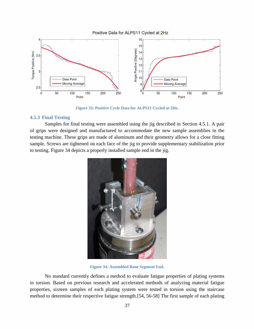
37
Figure 33: Positive Cycle Data for ALPS11 Cycled at 2Hz.
4.5.3 Final Testing
Samples for final testing were assembled using the jig described in Section 4.5.1. A pair
of grips were designed and manufactured to accommodate the new sample assemblies in the
testing machine. These grips are made of aluminum and their geometry allows for a close fitting
sample. Screws are tightened on each face of the jig to provide supplementary stabilization prior
to testing. Figure 34 depicts a properly installed sample end in the jig.
Figure 34: Assembled Bone Segment End.
No standard currently defines a method to evaluate fatigue properties of plating systems
in torsion. Based on previous research and accelerated methods of analyzing material fatigue
properties, sixteen samples of each plating system were tested in torsion using the staircase
method to determine their respective fatigue strength.[54, 56-58] The first sample of each plating

38
system was cycled at 1Hz to 60% of its previously determined acute failure torque, and all
samples were cycled 15,000 times.[50] After implanting a plating system, the patient is
recommended to remain under cage rest for the first six to eight weeks with activity limited to
five minutes a day. Based on gait analysis, 15,000 cycles represents an estimated number of
strides a canine will load onto the healing bone during six weeks of limited activity.[59] As seen
in previous studies, samples were torqued about the center axis of the bone model.[52, 60, 61]
One cycle is defined as torqueing the sample from its neutral position to the specified torque in
the positive direction, returning past the neutral position to the specified torque in the negative
direction, and back to its neutral position. The cycling torque for subsequent tests was increased
by 10% if run-out was achieved or decreased by 10% if the sample failed. To assist in
determining run-out or failure, maximum torque and angular displacement were recorded and
plotted for each half cycle of the test. After collaborating with veterinarians, three failure criteria
were defined before initiating the tests. Failure was considered if total angular rotation
progressively increased by at least 25% of its original value at the end of the test. This was
chosen as any higher angular rotation would have a greater chance of improperly healing. When
viewing the plot of total angular rotation per each half cycle, abrupt increases in angular rotation
were translated to sample failure as this depicts fracture in the system. Finally, if any visual
fracture of the bone plate, bone screws, or bone model were observed, the test was terminated
early and the sample was labeled as a failure. These criteria were established to ensure evaluation
of the plating systems with no addition fracture points or deformation. All samples and data were
also evaluated with veterinarians to confirm run-out and failure presence. Sixteen samples were
tested for each plating system.
4.5.4 Results
After testing is complete for each plating system sample, the acquired data and physical
integrity of the construct are analyzed to determine run-out or failure. When data portray sample
failure or fracture to the sample causes a premature end to the test, the construct is visually
inspected to determine the root cause. We expect to visualize failure in the form of screw pullout,
screw failure, bone model fracture, bone model failure, and plate failure. Screw pullout is
defined as the loosening or backing out of a screw from the plate as a result of cyclic loading.
Screw failure is defined as breakage of screws into two or more pieces. Bone model fracture is
defined as an intact construct only containing cracks on the bone model. Finally, bone model
failure is defined as breakage of a bone model into two or more pieces.
After testing is complete for each of the sixteen samples tested per plating system, a chart
is developed summarizing each the run-out and failure points at the various load levels. A sample
chart is seen in Figure 35.
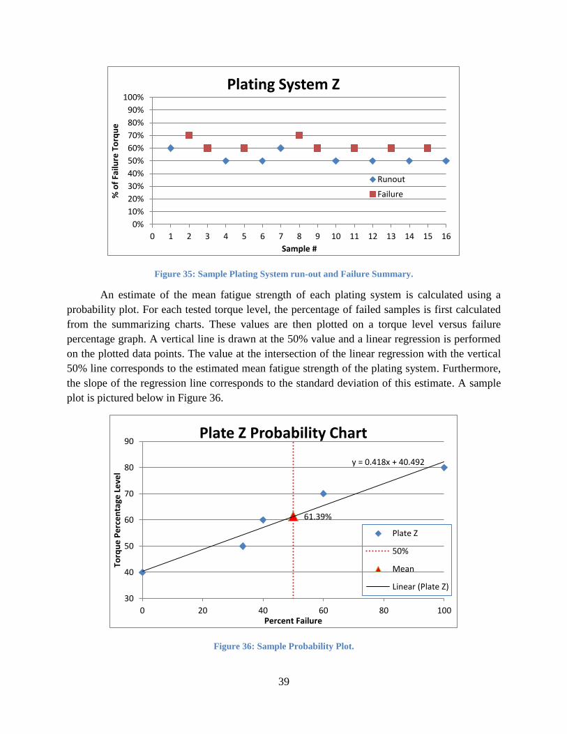
39
Figure 35: Sample Plating System run-out and Failure Summary.
An estimate of the mean fatigue strength of each plating system is calculated using a
probability plot. For each tested torque level, the percentage of failed samples is first calculated
from the summarizing charts. These values are then plotted on a torque level versus failure
percentage graph. A vertical line is drawn at the 50% value and a linear regression is performed
on the plotted data points. The value at the intersection of the linear regression with the vertical
50% line corresponds to the estimated mean fatigue strength of the plating system. Furthermore,
the slope of the regression line corresponds to the standard deviation of this estimate. A sample
plot is pictured below in Figure 36.
Figure 36: Sample Probability Plot.
0%
10%
20%
30%
40%
50%
60%
70%
80%
90%
100%
0 1 2 3 4 5 6 7 8 9 10 11 12 13 14 15 16
% o
f Fa
ilure
To
rqu
e
Sample #
Plating System Z
Runout
Failure
61.39%
y = 0.418x + 40.492
30
40
50
60
70
80
90
0 20 40 60 80 100
Torq
ue
Pe
rce
nta
ge L
eve
l
Percent Failure
Plate Z Probability Chart
Plate Z
50%
Mean
Linear (Plate Z)

40
The Dixon-Mood method is the more common technique used to estimate the mean and
standard deviation of fatigue strength.[54, 57] Enumerating run-outs and failures of each plating
system is first completed. The more prominent occurrence is used to perform the calculations. In
the event that the number of run-outs equals the number of failures, either group may be used as
they will yield the same results. Equation 4 below defines the variables A, B, and C required in
the Dixon-Mood equations.
Equation 4: A, B, and C variables for Dixon-Mood Equations.
∑
∑
∑
Load level is denoted as the integer parameter i in these equations with imax corresponding
to the highest stress level in the staircase. Stress level i = 0 corresponds to the lowest stress level
where run-out is observed if a majority of samples in the plating system failed. Conversely, i = 0
would correspond to the lowest stress level where failure is observed if a majority of samples in
the plating system achieved run-out. For example, if 9 of 16 samples failed with the lowest
survival load at 40% of the plating system’s failure torque, i = 0 would correspond to the 40%
level. If the step level in the staircase was 10% and the highest load level was 90%, imax would
equal five.
Equation 5 below defines the Dixon-Mood equation for mean fatigue strength in which
A, B, and C are inserted. Fatigue strength is defined as µ, initial load level is S0, and step size is
s. The plus sign in the equation is used when failures are the more prominent occurrence while
the minus sign is used when the opposite holds true.
Equation 5: Dixon-Mood Equation for Mean Fatigue Strength.
(
)
The Dixon-Mood method for calculating standard deviation is defined below in Equation
6 as variable σ.
Equation 6: Dixon-Mood Equation for Standard Deviation.
(
)
A table is created to more simply calculate the A, B, and C values which will be inserted
into the Dixon and Mood equations for mean fatigue strength and standard deviation. Load levels
are placed in descending order in column i. A second column is created noting the occurrences in
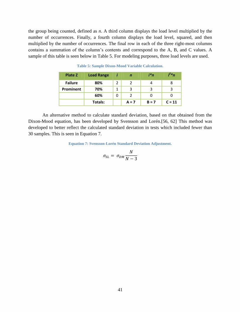
41
the group being counted, defined as n. A third column displays the load level multiplied by the
number of occurrences. Finally, a fourth column displays the load level, squared, and then
multiplied by the number of occurrences. The final row in each of the three right-most columns
contains a summation of the column’s contents and correspond to the A, B, and C values. A
sample of this table is seen below in Table 5. For modeling purposes, three load levels are used.
Table 5: Sample Dixon-Mood Variable Calculation.
Plate Z Load Range i n i*n i2*n
Failure 80% 2 2 4 8
Prominent 70% 1 3 3 3
60% 0 2 0 0
Totals: A = 7 B = 7 C = 11
An alternative method to calculate standard deviation, based on that obtained from the
Dixon-Mood equation, has been developed by Svensson and Lorén.[56, 62] This method was
developed to better reflect the calculated standard deviation in tests which included fewer than
30 samples. This is seen in Equation 7.
Equation 7: Svensson-Lorén Standard Deviation Adjustment.

42
5. Results
5.1 Four-point Bending
Raw data were recorded as comma separated variables. Three variables were reported:
time, displacement, and force. This data were analyzed using Microsoft Excel 2010, MATLAB
R2010b and Minitab Release 16. Calculations were made with the assistance of the ASTM F382
standard test methods for metallic bone plates. These methods describe the process for testing
metallic bone plates via four-point bending and extrapolation of bending stiffness, bending
structural stiffness, and bending strength properties as described in Section 4.4.1. The load
required to achieve plastic deformation in each plating system ranged from 150.0N to 580.4N.
The bending stiffness of each plating system ranged from 37.2N/mm to 98.2N/mm. The bending
strength of each plating system ranged from 3.8N-mm to 12.5N-mm. The bending structural
stiffness of each plating system ranged from 4.03Nm2 to 10.64Nm
2. The load-displacement
curves with calculated proof load are summarized in Appendix A. The mean and standard
deviation of these mechanical properties were calculated for each plating system and are
summarized in Table 6 below while the calculated data are elaborated in Appendix B. A one-way
ANOVA with Tukey pairwise comparison was conducted to determine which plating systems
had significantly different means when comparing their bending stiffness, bending strength, and
bending structural stiffness.
Table 6: Four-Point Bending Mechanical Property Summary.
Plating System Bending Stiffness (N/mm)
Bending Structural Stiffness (N-m2)
Bending Strength (N-mm)
Mean SD Mean SD Mean SD
DCP 71.0 15.2 7.7 1.7 9.6 2.1
LCDCP 57.3 1.3 6.2 0.1 8.5 0.4
Ti-LCDCP 44.2 2.6 4.8 0.3 6.1 0.6
LCP 66.7 6.6 7.2 0.7 6.7 2.1
ALPS10 40.0 1.9 4.3 0.2 5.1 1.2
ALPS11 76.3 1.8 8.3 0.2 11.6 0.6
SOP 80.4 12.5 8.7 1.4 11.6 1.7
Fixin 44.4 2.8 4.8 0.3 7.3 1.4
When comparing bending stiffnesses, DCP was significantly different from Ti LC-DCP,
ALPS10, and Fixin. LC-DCP was significantly different from SOP. Ti LC-DCP was
significantly different from LCP, ALPS11, and SOP. LCP was significantly different from
ALPS10 and Fixin. ALPS10 was significantly different from ALPS11 and SOP. Finally,
ALPS11 and SOP were both significantly different from Fixin. This is summarized in Table 7.
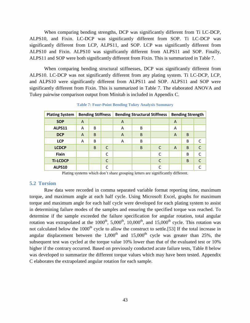
43
When comparing bending strengths, DCP was significantly different from Ti LC-DCP,
ALPS10, and Fixin. LC-DCP was significantly different from SOP. Ti LC-DCP was
significantly different from LCP, ALPS11, and SOP. LCP was significantly different from
ALPS10 and Fixin. ALPS10 was significantly different from ALPS11 and SOP. Finally,
ALPS11 and SOP were both significantly different from Fixin. This is summarized in Table 7.
When comparing bending structural stiffnesses, DCP was significantly different from
ALPS10. LC-DCP was not significantly different from any plating system. Ti LC-DCP, LCP,
and ALPS10 were significantly different from ALPS11 and SOP. ALPS11 and SOP were
significantly different from Fixin. This is summarized in Table 7. The elaborated ANOVA and
Tukey pairwise comparison output from Minitab is included in Appendix C.
Table 7: Four-Point Bending Tukey Analysis Summary
Plating System Bending Stiffness Bending Structural Stiffness Bending Strength
SOP A
A
A
ALPS11 A B
A B
A
DCP A B
A B
A B
LCP A B
A B
B C
LCDCP
B C
B C A B C
Fixin
C
C
B C
Ti-LCDCP
C
C
B C
ALPS10
C
C
C
Plating systems which don’t share grouping letters are significantly different.
5.2 Torsion
Raw data were recorded in comma separated variable format reporting time, maximum
torque, and maximum angle at each half cycle. Using Microsoft Excel, graphs for maximum
torque and maximum angle for each half cycle were developed for each plating system to assist
in determining failure modes of the samples and ensuring the specified torque was reached. To
determine if the sample exceeded the failure specification for angular rotation, total angular
rotation was extrapolated at the 1000th
, 5,000th
, 10,000th
, and 15,000th
cycle. This rotation was
not calculated below the 1000th
cycle to allow the construct to settle.[53] If the total increase in
angular displacement between the 1,000th
and 15,000th
cycle was greater than 25%, the
subsequent test was cycled at the torque value 10% lower than that of the evaluated test or 10%
higher if the contrary occurred. Based on previously conducted acute failure tests, Table 8 below
was developed to summarize the different torque values which may have been tested. Appendix
C elaborates the extrapolated angular rotation for each sample.

44
Table 8: Plating System Torque Values.
Plating System Torque Values (N-m)
100% 90% 80% 70% 60% 50% 40% 30% 20% 10%
SOP 8.66 7.79 6.93 6.06 5.20 4.33 3.46 2.60 1.73 0.87
LCP 8.53 7.68 6.82 5.97 5.12 4.27 3.41 2.56 1.71 0.85
ALPS11 8.35 7.52 6.68 5.85 5.01 4.18 3.34 2.51 1.67 0.84
DCP 8.32 7.49 6.66 5.82 4.99 4.16 3.33 2.50 1.66 0.83
LC-DCP 7.58 6.82 6.06 5.31 4.55 3.79 3.03 2.27 1.52 0.76
Fixin 6.80 6.12 5.44 4.76 4.08 3.40 2.72 2.04 1.36 0.68
ALPS10 5.68 5.11 4.54 3.98 3.41 2.84 2.27 1.70 1.14 0.57
When total angular displacement increased by 25% throughout the test, bone model
fracture, at minimum, was evident. When tested samples failed before reaching 15,000 cycles,
samples were visually inspected to determine the cause of failure. Screw fracture was evident
across all plating systems. Multiple plating systems also experienced bone model fracture and
failure. Screw pullout was only evident on one plating system, as was plate fracture. Table 9
summarizes the number of occurrences for each construct failure mode.
Table 9: Plating System Failure Mode Occurrences.
Screw Pullout
Screw Fracture
Bone Model Fracture
Bone Model Failure
Plate Failure
DCP
Occ
urr
ence
s
3 3 4
LCP 7 2
Fixin 8
ALPS10 1 1 6
ALPS11 5 7
SOP 1 9
LC-DCP 1 3 5
The run-out and failure data points for samples of each plating system were plotted to
note any visible trends in the data and are included in Appendix D. Appendix E includes the
summarized angular rotation, in degrees, for each plating system across four points throughout
the cycle. Probability plots were developed as one method of quantifying the estimated mean
fatigue strength and standard deviation of each plating system. These can be seen in Appendix F.
The previously described Dixon-Mood equations were also used as an equivalent method
for calculating mean fatigue strength and standard deviation. Mean fatigue strength was
calculated in terms of each plating system’s acute failure torque percentage and absolute torque
value in both methods. The highest mean fatigue strength in terms of percentage of acute failure
torque of the plating system able to survive at its highest percentage of acute torque was
observed in the ALPS10 plating system. The lowest was seen in the SOP plating system. Dixon-
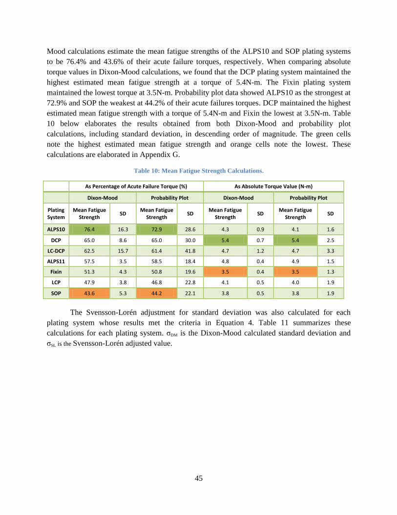
45
Mood calculations estimate the mean fatigue strengths of the ALPS10 and SOP plating systems
to be 76.4% and 43.6% of their acute failure torques, respectively. When comparing absolute
torque values in Dixon-Mood calculations, we found that the DCP plating system maintained the
highest estimated mean fatigue strength at a torque of 5.4N-m. The Fixin plating system
maintained the lowest torque at 3.5N-m. Probability plot data showed ALPS10 as the strongest at
72.9% and SOP the weakest at 44.2% of their acute failures torques. DCP maintained the highest
estimated mean fatigue strength with a torque of 5.4N-m and Fixin the lowest at 3.5N-m. Table
10 below elaborates the results obtained from both Dixon-Mood and probability plot
calculations, including standard deviation, in descending order of magnitude. The green cells
note the highest estimated mean fatigue strength and orange cells note the lowest. These
calculations are elaborated in Appendix G.
Table 10: Mean Fatigue Strength Calculations.
As Percentage of Acute Failure Torque (%) As Absolute Torque Value (N-m)
Dixon-Mood Probability Plot Dixon-Mood Probability Plot
Plating System
Mean Fatigue Strength
SD Mean Fatigue
Strength SD
Mean Fatigue Strength
SD Mean Fatigue
Strength SD
ALPS10 76.4 16.3 72.9 28.6 4.3 0.9 4.1 1.6
DCP 65.0 8.6 65.0 30.0 5.4 0.7 5.4 2.5
LC-DCP 62.5 15.7 61.4 41.8 4.7 1.2 4.7 3.3
ALPS11 57.5 3.5 58.5 18.4 4.8 0.4 4.9 1.5
Fixin 51.3 4.3 50.8 19.6 3.5 0.4 3.5 1.3
LCP 47.9 3.8 46.8 22.8 4.1 0.5 4.0 1.9
SOP 43.6 5.3 44.2 22.1 3.8 0.5 3.8 1.9
The Svensson-Lorén adjustment for standard deviation was also calculated for each
plating system whose results met the criteria in Equation 4. Table 11 summarizes these
calculations for each plating system. σDM is the Dixon-Mood calculated standard deviation and
σSL is the Svensson-Lorén adjusted value.

46
Table 11: Dixon-Mood and Svensson-Loren Standard Deviation Comparison.
Dixon-Mood and Svensson-Loren Standard Deviation Comparison
Failure Torque As: Percentage (%) Absolute Value (N-m)
Plating System σDM σSL σDM σSL
ALPS10 16.3 20.1 0.9 1.1
ALPS11 3.5 4.3 0.4 0.5
DCP 8.6 10.6 0.7 0.9
Fixin 4.3 5.3 0.4 0.4
LCP 3.8 4.7 0.5 0.6
LC-DCP 15.7 19.3 1.2 1.5
SOP 5.3 6.5 0.5 0.6

47
6. Discussion
6.1 Four-Point Bending
A few observations were made about the effect of bending forces on tested constructs.
With exception to Fixin, which has a flat underside, all plating systems have uniquely scalloped
or curved undersides with distinct lateral geometries. These features, in combination with evenly
spaced screw holes spanning across the entire length of the plate, influence the areas of
deformation in each plate when exposed to bending forces. These geometries can be observed
through two general design concepts. While not always the case, plates may incorporate wide
sections to accommodate screws with narrow connecting features. Furthermore, plates can have
scallops or other unique underside geometries in combination with a thicker profile at screw
holes and thinner profile at connecting segments. Deformation is guided to these narrower and
thinner sections as their smaller cross-sectional area results in a lower moment of inertia. This
lower moment of inertia corresponds to lower resistance to bending. Figure 37 below shows a
sample of each bone construct when loaded to the machine’s deflection limits via four-point
bending. Deformation is evident along the screw holes on the plate. These observations are
similar to those found in a study conducted by DeTora and Kraus.[35]
Figure 37: Four-point bending plate deformation. From left to right: DCP, LCP, SS LC-DCP, Ti LC-DCP,
ALPS11, ALPS10, Fixin, and SOP.
With exception to the Fixin plating system, no fracture was found to any plate, screw, or
bone model. Due to the geometry of the Fixin plate, we found that loads applied to the system
during four point bending induced a minor crack at the interface between the bone model and
plate at the fracture gap in one sample and catastrophic bone model fracture in a second sample.
This can be seen in Figure 38 and Figure 39. We attribute this partly to its flat underside as this
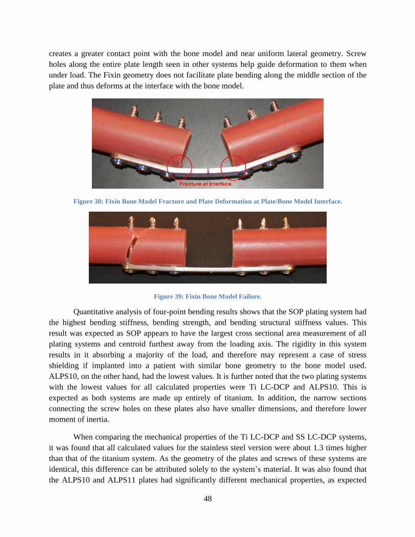
48
creates a greater contact point with the bone model and near uniform lateral geometry. Screw
holes along the entire plate length seen in other systems help guide deformation to them when
under load. The Fixin geometry does not facilitate plate bending along the middle section of the
plate and thus deforms at the interface with the bone model.
Figure 38: Fixin Bone Model Fracture and Plate Deformation at Plate/Bone Model Interface.
Figure 39: Fixin Bone Model Failure.
Quantitative analysis of four-point bending results shows that the SOP plating system had
the highest bending stiffness, bending strength, and bending structural stiffness values. This
result was expected as SOP appears to have the largest cross sectional area measurement of all
plating systems and centroid furthest away from the loading axis. The rigidity in this system
results in it absorbing a majority of the load, and therefore may represent a case of stress
shielding if implanted into a patient with similar bone geometry to the bone model used.
ALPS10, on the other hand, had the lowest values. It is further noted that the two plating systems
with the lowest values for all calculated properties were Ti LC-DCP and ALPS10. This is
expected as both systems are made up entirely of titanium. In addition, the narrow sections
connecting the screw holes on these plates also have smaller dimensions, and therefore lower
moment of inertia.
When comparing the mechanical properties of the Ti LC-DCP and SS LC-DCP systems,
it was found that all calculated values for the stainless steel version were about 1.3 times higher
than that of the titanium system. As the geometry of the plates and screws of these systems are
identical, this difference can be attributed solely to the system’s material. It was also found that
the ALPS10 and ALPS11 plates had significantly different mechanical properties, as expected
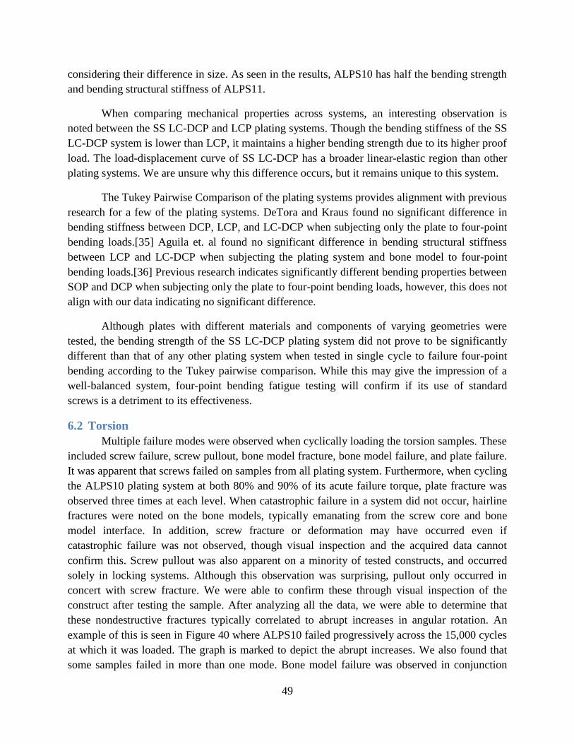
49
considering their difference in size. As seen in the results, ALPS10 has half the bending strength
and bending structural stiffness of ALPS11.
When comparing mechanical properties across systems, an interesting observation is
noted between the SS LC-DCP and LCP plating systems. Though the bending stiffness of the SS
LC-DCP system is lower than LCP, it maintains a higher bending strength due to its higher proof
load. The load-displacement curve of SS LC-DCP has a broader linear-elastic region than other
plating systems. We are unsure why this difference occurs, but it remains unique to this system.
The Tukey Pairwise Comparison of the plating systems provides alignment with previous
research for a few of the plating systems. DeTora and Kraus found no significant difference in
bending stiffness between DCP, LCP, and LC-DCP when subjecting only the plate to four-point
bending loads.[35] Aguila et. al found no significant difference in bending structural stiffness
between LCP and LC-DCP when subjecting the plating system and bone model to four-point
bending loads.[36] Previous research indicates significantly different bending properties between
SOP and DCP when subjecting only the plate to four-point bending loads, however, this does not
align with our data indicating no significant difference.
Although plates with different materials and components of varying geometries were
tested, the bending strength of the SS LC-DCP plating system did not prove to be significantly
different than that of any other plating system when tested in single cycle to failure four-point
bending according to the Tukey pairwise comparison. While this may give the impression of a
well-balanced system, four-point bending fatigue testing will confirm if its use of standard
screws is a detriment to its effectiveness.
6.2 Torsion
Multiple failure modes were observed when cyclically loading the torsion samples. These
included screw failure, screw pullout, bone model fracture, bone model failure, and plate failure.
It was apparent that screws failed on samples from all plating system. Furthermore, when cycling
the ALPS10 plating system at both 80% and 90% of its acute failure torque, plate fracture was
observed three times at each level. When catastrophic failure in a system did not occur, hairline
fractures were noted on the bone models, typically emanating from the screw core and bone
model interface. In addition, screw fracture or deformation may have occurred even if
catastrophic failure was not observed, though visual inspection and the acquired data cannot
confirm this. Screw pullout was also apparent on a minority of tested constructs, and occurred
solely in locking systems. Although this observation was surprising, pullout only occurred in
concert with screw fracture. We were able to confirm these through visual inspection of the
construct after testing the sample. After analyzing all the data, we were able to determine that
these nondestructive fractures typically correlated to abrupt increases in angular rotation. An
example of this is seen in Figure 40 where ALPS10 failed progressively across the 15,000 cycles
at which it was loaded. The graph is marked to depict the abrupt increases. We also found that
some samples failed in more than one mode. Bone model failure was observed in conjunction
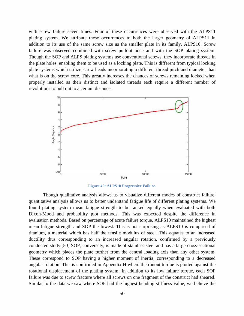
50
with screw failure seven times. Four of these occurrences were observed with the ALPS11
plating system. We attribute these occurrences to both the larger geometry of ALPS11 in
addition to its use of the same screw size as the smaller plate in its family, ALPS10. Screw
failure was observed combined with screw pullout once and with the SOP plating system.
Though the SOP and ALPS plating systems use conventional screws, they incorporate threads in
the plate holes, enabling them to be used as a locking plate. This is different from typical locking
plate systems which utilize screw heads incorporating a different thread pitch and diameter than
what is on the screw core. This greatly increases the chances of screws remaining locked when
properly installed as their distinct and isolated threads each require a different number of
revolutions to pull out to a certain distance.
Figure 40: ALPS10 Progressive Failure.
Though qualitative analysis allows us to visualize different modes of construct failure,
quantitative analysis allows us to better understand fatigue life of different plating systems. We
found plating system mean fatigue strength to be ranked equally when evaluated with both
Dixon-Mood and probability plot methods. This was expected despite the difference in
evaluation methods. Based on percentage of acute failure torque, ALPS10 maintained the highest
mean fatigue strength and SOP the lowest. This is not surprising as ALPS10 is comprised of
titanium, a material which has half the tensile modulus of steel. This equates to an increased
ductility thus corresponding to an increased angular rotation, confirmed by a previously
conducted study.[50] SOP, conversely, is made of stainless steel and has a large cross-sectional
geometry which places the plate further from the central loading axis than any other system.
These correspond to SOP having a higher moment of inertia, corresponding to a decreased
angular rotation. This is confirmed in Appendix H where the runout torque is plotted against the
rotational displacement of the plating system. In addition to its low failure torque, each SOP
failure was due to screw fracture where all screws on one fragment of the construct had sheared.
Similar to the data we saw where SOP had the highest bending stiffness value, we believe the
51
failure mode of this system’s fatigue testing in torsion further support the idea that this system
has a high potential to cause stress shielding and be detriment to fracture healing. Although the
Fixin plating system also failed due to screw fracture, we do not believe this is due to stress
shielding. The shape of the plate deflects a majority of the angular rotation to the interface
between the plate and the bone model and transfers much of this energy to the screws, thereby
causing screw fracture across the tested cycle.
Higher angular rotation corresponds to a less stiff system and a lower angular rotation to
a stiffer system. When the system is more ductile, as in the case with ALPS10, the plate is able to
absorb more of the energy, thus removing some stresses present at the plate and screw interface.
This corresponds to a lower susceptibility of screw fracture. Only one sample failed due to screw
fracture with ALPS10, whereas it was the cause for failure in nine of the SOP samples. It is
observed that the two plating systems comprised of titanium, ALPS10 and ALPS11, generally
have a greater rotational displacement than the stainless steel plating systems across overlapping
torque ranges. We are unsure of the impact of monocortical screw use in vivo as cyclic loading
caused erosion of the bone model at the screw interface. By calculating the percentage of the
failure torque a plating system is able to sustain, we can see how its material and geometry
impacts its ability to be cyclically loaded.
When comparing absolute torque values, DCP proved to be the strongest and Fixin the
weakest. We expected this considering the Fixin plating system has the smallest cross-sectional
area of all plating systems. When comparing dimensions of the DCP, LCP, and LC-DCP plating
systems, we found their width and height to be identical, though their screw hole patterns and
underside geometries differed. We attribute the higher mean fatigue strength of the DCP
construct to its greater cross-sectional area as its underside geometry is uniform when compared
to the LCP and LC-DCP plating systems. This further allowed increased contact at the plate and
bone model interface. While the DCP system employs the highest absolute fatigue strength, its
clinical use may not be ideal due to non-locking screws and increased blood supply interference.
We also note that DCP maintained the second strongest plating system when comparing
percentage of acute failure torque, though ALPS10 maintained the median absolute torque value.
By calculating the absolute torque values sustained by each system, we are able to compare them
all regardless of their geometry. However, this cannot outline the effects of stress shielding as
each plating system was able to maintain different angular rotations.
LCP and LC-DCP have similar, though not equal, failure torques. Based on the measured
angular rotation in each construct at equal load levels, as seen in Appendix E:, LCP demonstrates
a higher total angular rotation in comparison to LC-DCP and therefore a lower resistance to
cyclic torsion loading. This aligns with previous research indicating LCP is less resistant to
cyclic torsion loads in comparison to LC-DCP when secured to a bone model.[53] Depending on
the activity level of the patient, angular rotation of the system can play a role in fracture healing.
Although activity should be restricted during the first six to eight weeks after implantation, those
52
that are more active and able to transfer higher loads to the fractured bone may benefit from a
stiffer plate to limit angular rotation as excessive movement can lead to delayed or non-union.
Probability plots and the Dixon-Mood method are the only methods of analyzing
staircase data. The accuracy of probability plots are directly proportional to the number of torque
levels at which the samples have been tested as the calculated mean fatigue strength is dependent
on the goodness of fit of the linear regression. Estimated mean fatigue strength using both
probability plots and Dixon and Mood equations seem to be similar, though the calculated
standard deviations vary greatly. Unfortunately, we are unable to statistically quantify the
correlation between the values acquired through the two evaluation methods. We believe that the
probability plots have a higher standard deviation due to the low number of tested torque levels.
While standard deviation calculated from the Dixon-Mood equations appear to be more accurate,
the research of Svensson and Lorén makes particular note to the need for more accurate standard
deviation calculations when testing small sample sizes. This is the motive behind the
supplementary calculation to the Dixon-Mood results. It is evident from the Svensson-Lorén
results that a higher standard deviation is calculated in all applicable plating systems in
comparison to the values acquired from the Dixon-Mood methods. This is expected as smaller
sample sizes may not always portray an accurate population mean and standard deviation.
Testing of supplementary constructs will allow us to create a more accurate calculation of both
fatigue strength and standard deviation.
A once-inch gap was chosen for the constructs to mimic a bridging osteosynthesis for a
comminuted fracture. This gap, in addition, more severely tests the differences in plate geometry
and securing methods due to the increased plating area lacking an interface with the bone model.
A limitation of this test setup is that the loading axis lies along the center of the bone model. If
each construct was assembled to mimic the true loading axis for each construct based on the
applied plating system’s geometry, more physiologically accurate results would be acquired. By
torqueing the plating systems along the center axis of the bone model, we were able to maintain a
uniform testing field throughout all samples, in addition to more severely stressing the plating
systems. The more physiologically accurate torqueing axis would be shifted away from the bone
center and toward the plate at a distance dependent on the plate’s centroid. Furthermore, this
setup does not portray the true effect of internal and external forces acting upon a fractured bone
as they typically act in a combination of torsion, bending, and shear modes and not pure
torsion.[48, 49] Thus, the calculated fatigue strength of these plating systems represents the
worst-case torsion loading conditions.
6.3 Cinical Relevance
Stiffness and relative rigidity of these plating systems provide a good indication of
systems which may contribute more to stress shielding than others, based on the results of our
quantitative analyses for both loading modes. However, based on our observations, plating
systems offer various design features which may promote or reduce healing ability.
53
Features reducing the contact area between the plate and the bone result in preserving the
blood supply at the fracture site and thus promote proper healing. The plates incorporating these
features include SS LC-DCP, Ti LC-DCP, LCP, ALPS10, ALPS11, and SOP. Furthermore,
locking plates provide the least disruption of the blood supply since no contact is required
between the plate and the bone.
As observed in the Fixin plating system, lacking screw holes across the entire length of
the plate deflects loads to the plate and bone interface rather than distributing the load more
evenly across the entire plate length. This feature, in addition to Fixin’s underside geometry
posing a high risk of disrupting the blood supply at the fracture site reduce its ability to properly
heal fractures.
Deformation in the other systems was relatively uniform, though most apparent along the
screw holes. ALPS10 and ALPS11 deformed most uniformly across the entire length of the plate
due to its unique geometric features. Based on the evaluated bending properties of these two
plating systems, ALPS11 maintains the second highest values and ALPS10 the lowest, thus
representing nearly the entire range of tested systems. Therefore, based on what we have
observed with regard to the bending profiles of the ALPS10 and ALPS11 plates, implementing
this design to create a range of stiffness properties based on the size of the patient and severity of
the fracture would be beneficial.
The unique geometry of the SOP system allows for it to be contoured with six degrees of
freedom when necessary without deforming the screw holes. However, due to the size of this
system, a majority of the load is absorbed by the plate and the stresses transferred to the screws,
leading to screw failure. Unless unique contouring is required or the geometry is updated to
better distribute the load, implanting an SOP system may not be the ideal choice for promoting
proper healing.
54
7. Conclusions
This focus of this study was to evaluate the mechanical properties of seven plating
systems using acute four-point bending and cyclic fatigue torsion test methods. The combination
of these forces has been shown to represent more than 90% of loads acting on a fracture, though
their exact mechanisms are not known.[48, 49] Based on the analyzed test data we are able to
conclude that the SOP system has the highest acute bending mechanical properties and ALPS10
the lowest. Analysis of the cyclic torsion fatigue data allows us to conclude that the ALPS10
system is able to maintain the highest percentage of its failure torque when tested to 15,000
cycles and SOP the lowest. Furthermore, the DCP system is able to maintain the highest absolute
torque value across 15,000 cycles and Fixin the lowest. The absolute torque data gives us an idea
of how the plating system’s material and geometry influence its cyclic behavior, although this
alone cannot determine the superior plating system as it does not account for effects of stress
shielding.
Based on qualitative analysis of the plating systems, several design features are beneficial
to the healing of fractures. By incorporating screw holes along with a unique geometry along the
entire length of the plate, plating system deformation as a result of bending loads can be made
more uniform and deflected away from the plate and bone interface. In addition, as preserving
the periosteum of the of the bone is critical to the reconstruction of bone, conventional plating
systems which reduce the contact with bone and locked plating systems which do not require
contact with bone are able to achieve this. Finally, although not preferred, if a complex plate
contour is required to properly heal bone, the pearls and internodes of the SOP plating system
offer a unique approach to contouring a plate without risk of deforming the screw holes.
The conducted mechanical evaluation is the start of better understanding plate mechanics.
To further develop and understand the mechanical properties of these plating systems, it is
recommended to perform fatigue life testing with both loading conditions. This should entail
cyclic testing in both torsion and four-point bending to at least one million cycles per sample.
This is recommended by ASTM F382 to accurately compare a plating system’s geometric and
material properties to its ability to resist fatigue. While the quantitative testing is an excellent
start to the evaluation of bone plating systems, we are still unable to make conclusions about
their effectiveness in vivo as biological responses were not examined. Controlled testing in vivo
will allow for more accurate determination of the shortcomings of each system in addition to
providing a more accurate understanding of a plating system’s mechanical and biological
response. Controlled in vivo testing will allow conclusions to be made regarding each system’s
effectiveness.
When considering application of a plating system on a comminuted canine femoral
fracture, the results reported in this study should be interpreted in concert with cyclic four-point
bending results and veterinary requirements.

55
Bibliography
1. Tan, S.L. and Z.J. Balogh, Indications and limitations of locked plating. Injury, 2009. 40(7):
p. 683-691.
2. Zlowodzki, M., et al., Operative treatment of acute distal femur fractures: systematic review
of 2 comparative studies and 45 case series (1989 to 2005). J Orthop Trauma, 2006. 20(5): p.
366-71.
3. Miller, D.L. and T. Goswami, A review of locking compression plate biomechanics and their
advantages as internal fixators in fracture healing. Clinical Biomechanics, 2007. 22(10): p.
1049-1062.
4. Carter, D.R., Mechanical loading histories and cortical bone remodeling. Calcified tissue
international, 1984. 36: p. 19-24.
5. Rüedi, T.P., et al., AO principles of fracture management. Vol. 1. 2007: George Thieme
Verlag.
6. Athanasiou, K.A., et al., Fundamentals of biomechanics in tissue engineering of bone. Tissue
engineering, 2000. 6(4): p. 361-381.
7. ASTM Standard F382, 2008e1, "Standard Specification and Test Method for Metallic Bone
Plates," ASTM International, West Conshohocken, PA, 2008.
8. Kemp, T., et al., Functional trade-offs in the limb bones of dogs selected for running versus
fighting. Journal of experimental biology, 2005. 208(18): p. 3475-3482.
9. Marsell, R. and T.A. Einhorn, The biology of fracture healing. Injury, 2011. 42(6): p. 551-
555.
10. Perren, S.M., Evolution of the internal fixation of long bone fractures: the scientific basis of
biological internal fixation: choosing a new balance between stability and biology. Journal
of Bone and Joint Surgery-British Volume, 2002. 84(8): p. 1093.
11. Jahagirdar, R. and B.E. Scammell, Principles of fracture healing and disorders of bone
union. Surgery (Oxford), 2009. 27(2): p. 63-69.
12. Ramakrishna, K., et al., Design of Fracture Fixation Plate for Necessary and Sufficient Bone
Stress Shielding. JSME International Journal Series C Mechanical Systems, Machine
Elements and Manufacturing, 2004. 47(4): p. 1086-1094.
13. Lindholm, R., et al., The mast cell as a component of callus in healing fractures. J Bone Joint
Surg Br, 1969. 51(1): p. 148-55.
14. Pape, H.C., et al., Effects of intramedullary femoral fracture fixation: what is the impact of
experimental studies in regards to the clinical knowledge? Shock, 2002. 18(4): p. 291-300.
15. Court-Brown, C.M., et al., Reamed or unreamed nailing for closed tibial fractures. A
prospective study in Tscherne C1 fractures. J Bone Joint Surg Br, 1996. 78(4): p. 580-3.
16. Haas, N., et al., A new solid unreamed tibial nail for shaft fractures with severe soft tissue
injury. Injury, 1993. 24(1): p. 49-54.
17. McKibbin, B., The biology of fracture healing in long bones. J Bone Joint Surg Br, 1978. 60-
B(2): p. 150-62.
18. Pearson, O.M. and D.E. Lieberman, The aging of Wolff's "law": ontogeny and responses to
mechanical loading in cortical bone. Am J Phys Anthropol, 2004. Suppl 39: p. 63-99.
19. Besdo, S., Determination of dynamically adapting anisotropic material properties of bone
under cyclic loading. J Biomech, 2011. 44(2): p. 272-6.
56
20. Robling, A.G., D.B. Burr, and C.H. Turner, Partitioning a Daily Mechanical Stimulus into
Discrete Loading Bouts Improves the Osteogenic Response to Loading. Journal of Bone and
Mineral Research, 2000. 15(8): p. 1596-1602.
21. Burr, D.B., A.G. Robling, and C.H. Turner, Effects of biomechanical stress on bones in
animals. Bone, 2002. 30(5): p. 781-6.
22. Huang, C. and R. Ogawa, Mechanotransduction in bone repair and regeneration. FASEB J,
2010. 24(10): p. 3625-32.
23. Datta, H.K., et al., The cell biology of bone metabolism. Journal of Clinical Pathology, 2008.
61(5): p. 577-587.
24. Cordey, J., S.M. Perren, and S.G. Steinemann, Stress protection due to plates: myth or
reality? A parametric analysis made using the composite beam theory. Injury, 2000. 31
Suppl 3: p. C1-13.
25. Tonino, A.J., et al., Protection from stress in bone and its effects. Experiments with stainless
steel and plastic plates in dogs. J Bone Joint Surg Br, 1976. 58(1): p. 107-13.
26. Krishna, K.R., I. Sridhar, and D.N. Ghista, Analysis of the helical plate for bone fracture
fixation. Injury, 2008. 39(12): p. 1421-36.
27. Stoffel, K., et al., Biomechanical testing of the LCP – how can stability in locked internal
fixators be controlled? Injury, 2003. 34, Supplement 2(0): p. 11-19.
28. Levine, R.S., Injury to the extremities. Accidental injury: biomechanics and prevention.
Nahum AM, Melvin J, eds. New York: Springer-Verlag, 1993: p. 460-492.
29. Pierce, M.C., et al., Evaluating long bone fractures in children: a biomechanical approach
with illustrative cases. Child Abuse Negl, 2004. 28(5): p. 505-24.
30. Turner, C.H. and D.B. Burr, Basic biomechanical measurements of bone: A tutorial. Bone,
1993. 14(4): p. 595-608.
31. Kress, T., et al. Fracture patterns of human cadaver long bones. 1995.
32. AO Surgery Reference. [cited 2012 June 25]; Available from: http://www2.aofoundation.org.
33. Stiffler, K.S., Internal fracture fixation. Clinical Techniques in Small Animal Practice, 2004.
19(3): p. 105-113.
34. Niemeyer, P. and N.P. Sudkamp, Principles and clinical application of the locking
compression plate (LCP). Acta Chir Orthop Traumatol Cech, 2006. 73(4): p. 221-228.
35. DeTora, M. and K. Kraus, Mechanical testing of 3.5 mm locking and non-locking bone
plates. Vet Comp Orthop Traumatol, 2008. 21(4): p. 318-22.
36. Aguila, A.Z., et al., In vitro biomechanical comparison of limited contat dynamic
compression plate and locking compression plate. Vet Comp Orthop Traumatol, 2005. 18(4):
p. 220-6.
37. Ness, M.G., The effect of bending and twisting on the stiffness and strength of the 3.5 SOP
implant. Vet Comp Orthop Traumatol, 2009. 22(2): p. 132-6.
38. Ness, M.G., Repair of Y-T humeral fractures in the dog using paired 'String of Pearls'
locking plates. Vet Comp Orthop Traumatol, 2009. 22(6): p. 492-7.
39. Petazzoni, M., et al., Fixin internal fixator: Concept and technique. VCOT, 2009. 22(4): p.
309-315.
40. Inauen, R., D. Koch, and M. Bass, Arthrodesis of the tarsometatarsal joints in a cat with a
two hole advanced locking plate system. Vet Comp Orthop Traumatol, 2009. 22(2): p. 166-9.
41. Kyon Veterinary Surgical Products. [cited 2012 May 1]; Available from:
http://www.kyon.ch.
57
42. Apivatthakakul, T., C. Phornphutkul, and S. Patumasutra, Idea and innovation: Simple
minimally invasive plate osteosynthesis (MIPO) instruments. Injury Extra, 2009. 40(2): p. 39-
44.
43. Patel, P.S.D., D.E.T. Shepherd, and D.W.L. Hukins, The effect of screw insertion angle and
thread type on the pullout strength of bone screws in normal and osteoporotic cancellous
bone models. Medical Engineering & Physics, 2010. 32(8): p. 822-828.
44. Augat, P., et al., Local tissue properties in bone healing: Influence of size and stability of the
osteotomy gap. Journal of Orthopaedic Research, 1998. 16(4): p. 475-481.
45. Markel, M.D., M.A. Wikenheiser, and E.Y.S. Chao, A study of fracture callus material
properties: Relationship to the torsional strength of bone. Journal of Orthopaedic Research,
1990. 8(6): p. 843-850.
46. Jepsen, K.J. and D.T. Davy, Comparison of damage accumulation measures in human
cortical bone. Journal of Biomechanics, 1997. 30(9): p. 891-894.
47. Gautier, E. and C. Sommer, Guidelines for the clinical application of the LCP. Injury, 2003.
34 Suppl 2: p. B63-76.
48. Stoffel, K., K. Klaue, and S.M. Perren, Functional load of plates in fracture fixation in vivo
and its correlate in bone healing. Injury, 2000. 31, Supplement 2(0): p. 37-86.
49. Gautier, E., S. Perren, and J. Cordey, Strain distribution in plated and unplated sheep tibia
an in vivo experiment. Injury, 2000. 31: p. 37-93.
50. Cabassu, J., et al., Single cycle to failure in torsion of three standard and five locking plate
constructs. Veterinary and Comparative Orthopaedics and Traumatology, 2011. 24(6): p.
418.
51. Acker ML, T.B., Kowaleski MP, Boudrieau RJ. Structural properties of synthetic bone
models compared to native canine bone. in European College of Veterinary Surgeons, 19th
Annual Scientific Meeting. 2010. Helsinki, Finland.
52. Fitzpatrick, D.C., et al., Relative stability of conventional and locked plating fixation in a
model of the osteoporotic femoral diaphysis. Clinical Biomechanics, 2009. 24(2): p. 203-209.
53. Filipowicz, D., et al., A biomechanical comparison of 3.5 locking compression plate fixation
to 3.5 limited contact dynamic compression plate fixation in a canine cadaveric distal
humeral metaphyseal gap model. Veterinary and Comparative Orthopaedics and
Traumatology, 2009. 22(4): p. 270-7.
54. Lin, S.K., Y.L. Lee, and M.W. Lu, Evaluation of the staircase and the accelerated test
methods for fatigue limit distributions. International journal of fatigue, 2001. 23(1): p. 75-83.
55. Lee, Y.L., Fatigue testing and analysis: theory and practice. Vol. 13. 2005: Butterworth-
Heinemann.
56. Pollak, R.D., Analysis of Methods for Determining High Cycle Fatigue Strength of a
Material With Investigation of Ti-6Al-4V Gigacycle Fatigue Behavior, 2005, DTIC
Document.
57. Nicholas, T., High cycle fatigue: a mechanics of materials perspective2006: Elsevier
Science.
58. Crow, E.L., F.A. Davis, and M.W. Maxfield, Statistics manual: with examples taken from
ordnance development. Vol. 3369. 1960: Dover Publications.
59. Hottinger, H.A., et al., Noninvasive kinematic analysis of the walk in healthy large-breed
dogs. Am J Vet Res, 1996. 57(3): p. 381-8.
60. Heiner, A.D. and T.D. Brown, Structural properties of a new design of composite replicate
femurs and tibias. Journal of Biomechanics, 2001. 34(6): p. 773-781.

58
61. Yánez, A., J.A. Carta, and G. Garcés, Biomechanical evaluation of a new system to improve
screw fixation in osteoporotic bones. Medical Engineering & Physics, 2010. 32(5): p. 532-
541.
62. Pollak, R., A. Palazotto, and T. Nicholas, A simulation-based investigation of the staircase
method for fatigue strength testing. Mechanics of Materials, 2006. 38(12): p. 1170-1181.
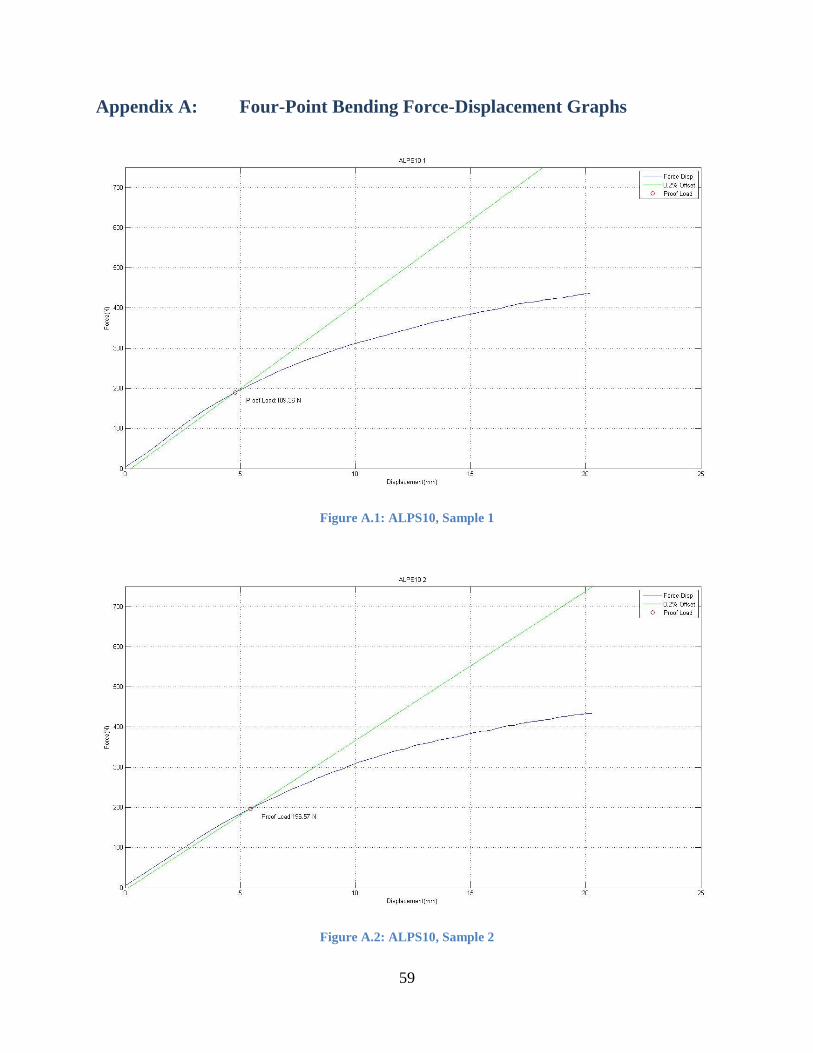
59
Appendix A: Four-Point Bending Force-Displacement Graphs
Figure A.1: ALPS10, Sample 1
Figure A.2: ALPS10, Sample 2

60
Figure A.3: ALPS10, Sample 3
Figure A.4: ALPS10, Sample 4

61
Figure A.5: ALPS11, Sample 1
Figure A.6: ALPS11, Sample 2
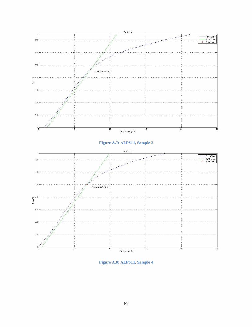
62
Figure A.7: ALPS11, Sample 3
Figure A.8: ALPS11, Sample 4

63
Figure A.9: DCP, Sample 1
Figure A.10: DCP, Sample 2

64
Figure A.11: DCP, Sample 3
Figure A.12: DCP, Sample 4
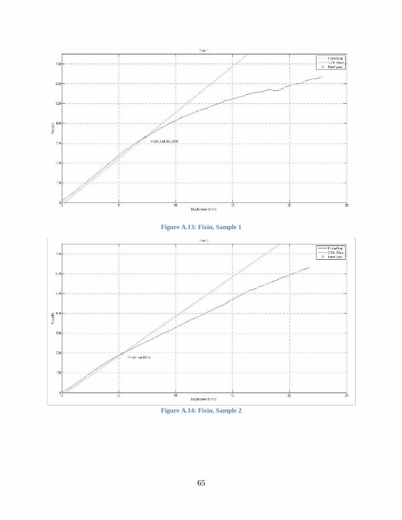
65
Figure A.13: Fixin, Sample 1
Figure A.14: Fixin, Sample 2
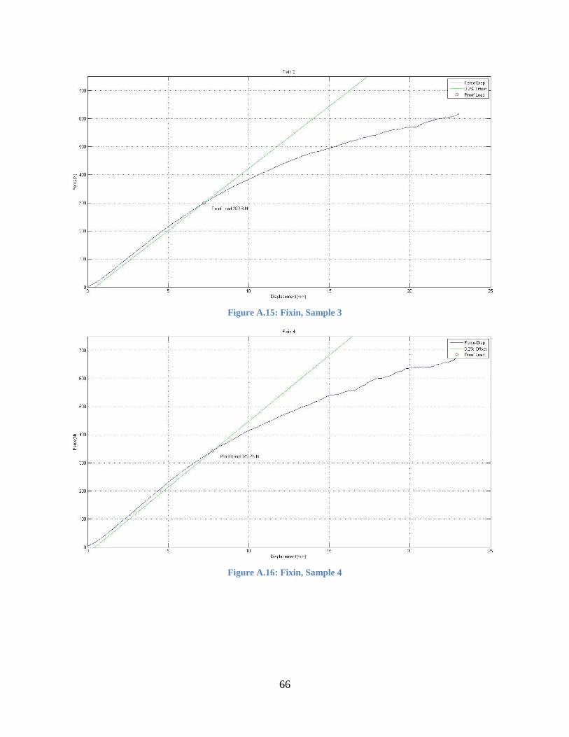
66
Figure A.15: Fixin, Sample 3
Figure A.16: Fixin, Sample 4
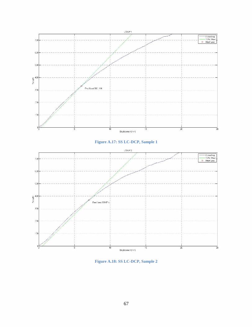
67
Figure A.17: SS LC-DCP, Sample 1
Figure A.18: SS LC-DCP, Sample 2
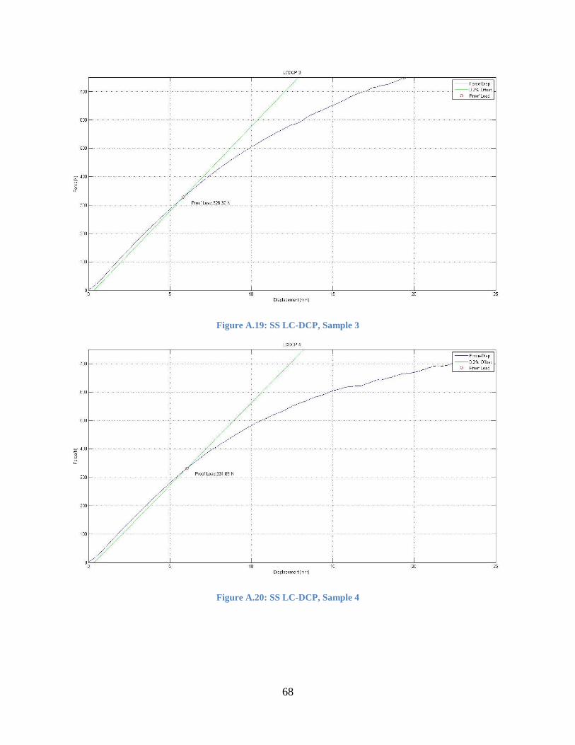
68
Figure A.19: SS LC-DCP, Sample 3
Figure A.20: SS LC-DCP, Sample 4
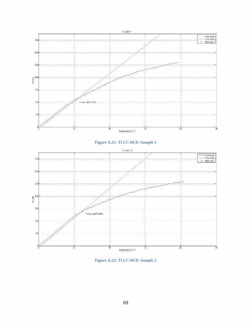
69
Figure A.21: Ti LC-DCP, Sample 1
Figure A.22: Ti LC-DCP, Sample 2

70
Figure A.23: Ti LC-DCP, Sample 3
Figure A.24: Ti LC-DCP, Sample 4
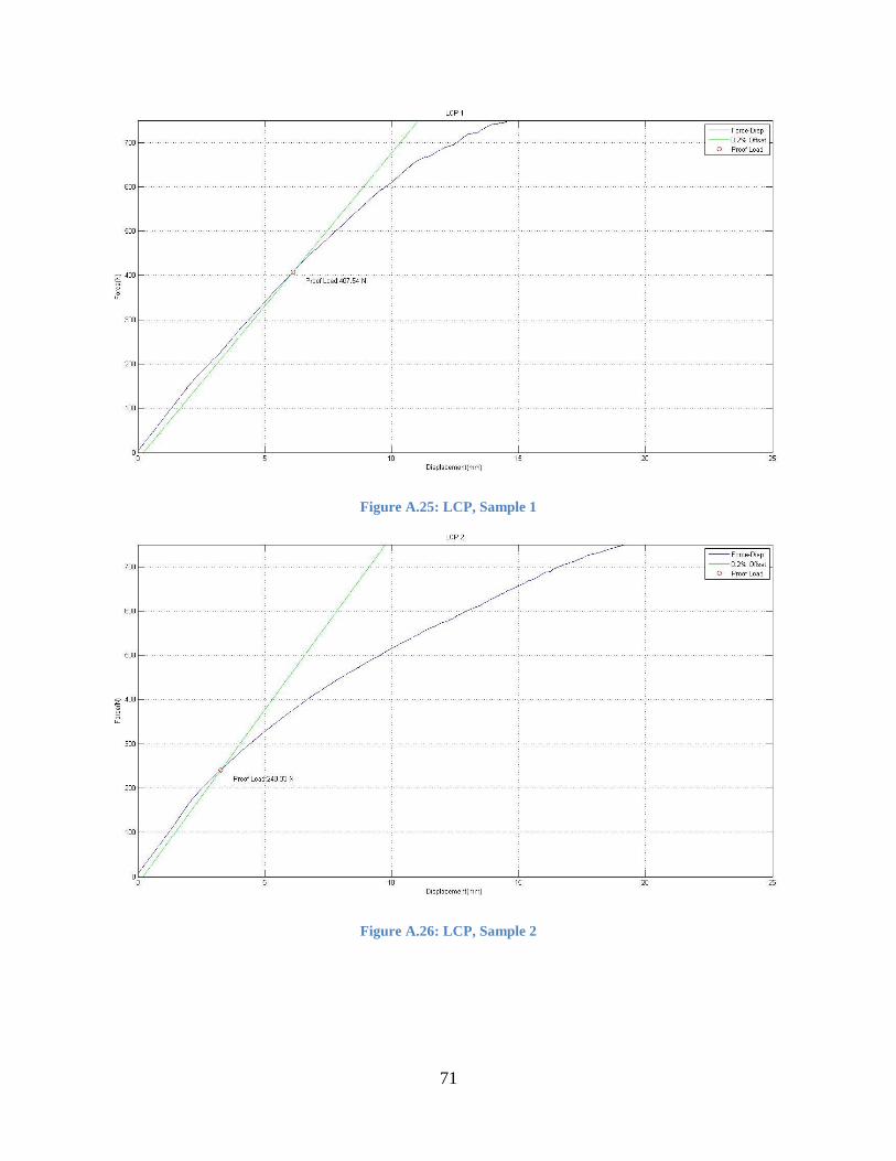
71
Figure A.25: LCP, Sample 1
Figure A.26: LCP, Sample 2

72
Figure A.27: LCP, Sample 3
Figure A.28: LCP, Sample 4

73
Figure A.29: SOP, Sample 1
Figure A.30: SOP, Sample 2
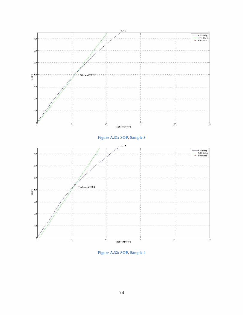
74
Figure A.31: SOP, Sample 3
Figure A.32: SOP, Sample 4
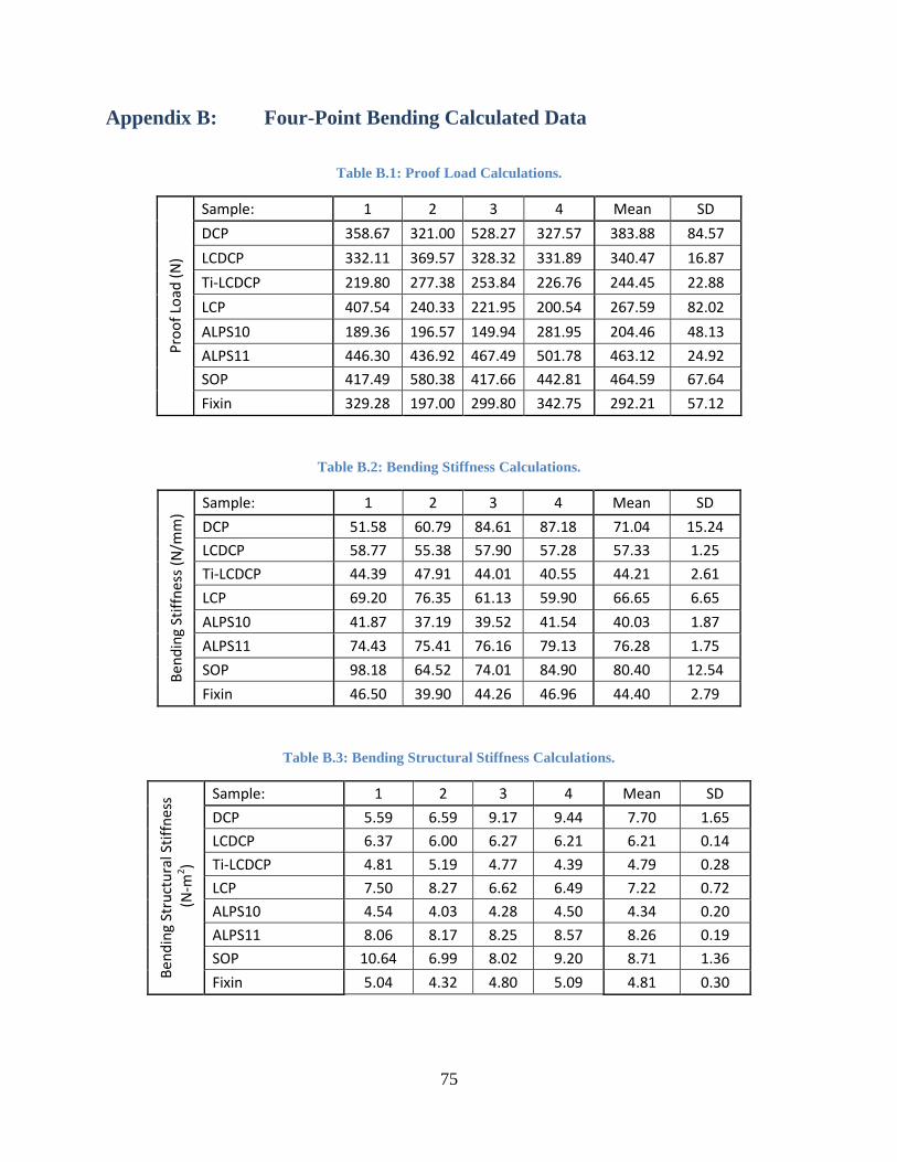
75
Appendix B: Four-Point Bending Calculated Data
Table B.1: Proof Load Calculations. P
roo
f Lo
ad (
N)
Sample: 1 2 3 4 Mean SD
DCP 358.67 321.00 528.27 327.57 383.88 84.57
LCDCP 332.11 369.57 328.32 331.89 340.47 16.87
Ti-LCDCP 219.80 277.38 253.84 226.76 244.45 22.88
LCP 407.54 240.33 221.95 200.54 267.59 82.02
ALPS10 189.36 196.57 149.94 281.95 204.46 48.13
ALPS11 446.30 436.92 467.49 501.78 463.12 24.92
SOP 417.49 580.38 417.66 442.81 464.59 67.64
Fixin 329.28 197.00 299.80 342.75 292.21 57.12
Table B.2: Bending Stiffness Calculations.
Ben
din
g St
iffn
ess
(N/m
m)
Sample: 1 2 3 4 Mean SD
DCP 51.58 60.79 84.61 87.18 71.04 15.24
LCDCP 58.77 55.38 57.90 57.28 57.33 1.25
Ti-LCDCP 44.39 47.91 44.01 40.55 44.21 2.61
LCP 69.20 76.35 61.13 59.90 66.65 6.65
ALPS10 41.87 37.19 39.52 41.54 40.03 1.87
ALPS11 74.43 75.41 76.16 79.13 76.28 1.75
SOP 98.18 64.52 74.01 84.90 80.40 12.54
Fixin 46.50 39.90 44.26 46.96 44.40 2.79
Table B.3: Bending Structural Stiffness Calculations.
Ben
din
g St
ruct
ura
l Sti
ffn
ess
(N
-m2 )
Sample: 1 2 3 4 Mean SD
DCP 5.59 6.59 9.17 9.44 7.70 1.65
LCDCP 6.37 6.00 6.27 6.21 6.21 0.14
Ti-LCDCP 4.81 5.19 4.77 4.39 4.79 0.28
LCP 7.50 8.27 6.62 6.49 7.22 0.72
ALPS10 4.54 4.03 4.28 4.50 4.34 0.20
ALPS11 8.06 8.17 8.25 8.57 8.26 0.19
SOP 10.64 6.99 8.02 9.20 8.71 1.36
Fixin 5.04 4.32 4.80 5.09 4.81 0.30
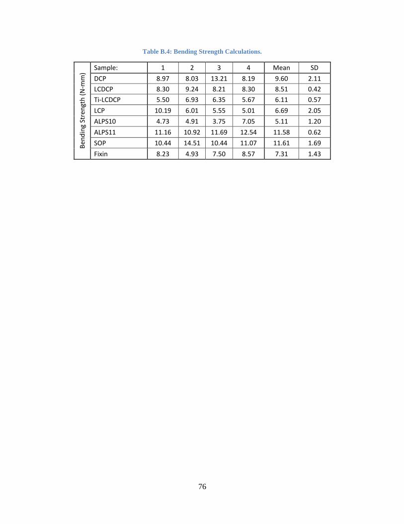
76
Table B.4: Bending Strength Calculations.
Ben
din
g St
ren
gth
(N
-mm
)
Sample: 1 2 3 4 Mean SD
DCP 8.97 8.03 13.21 8.19 9.60 2.11
LCDCP 8.30 9.24 8.21 8.30 8.51 0.42
Ti-LCDCP 5.50 6.93 6.35 5.67 6.11 0.57
LCP 10.19 6.01 5.55 5.01 6.69 2.05
ALPS10 4.73 4.91 3.75 7.05 5.11 1.20
ALPS11 11.16 10.92 11.69 12.54 11.58 0.62
SOP 10.44 14.51 10.44 11.07 11.61 1.69
Fixin 8.23 4.93 7.50 8.57 7.31 1.43
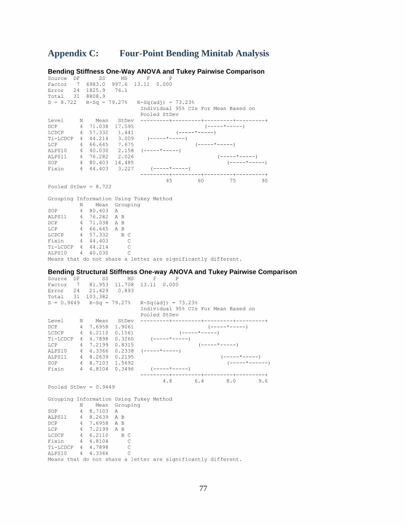
77
Appendix C: Four-Point Bending Minitab Analysis Bending Stiffness One-Way ANOVA and Tukey Pairwise Comparison Source DF SS MS F P
Factor 7 6983.0 997.6 13.11 0.000
Error 24 1825.9 76.1
Total 31 8808.9
S = 8.722 R-Sq = 79.27% R-Sq(adj) = 73.23%
Individual 95% CIs For Mean Based on
Pooled StDev
Level N Mean StDev ---------+---------+---------+---------+
DCP 4 71.038 17.595 (-----*-----)
LCDCP 4 57.332 1.441 (-----*-----)
Ti-LCDCP 4 44.214 3.009 (-----*-----)
LCP 4 66.645 7.675 (-----*-----)
ALPS10 4 40.030 2.158 (-----*-----)
ALPS11 4 76.282 2.026 (-----*-----)
SOP 4 80.403 14.485 (-----*-----)
Fixin 4 44.403 3.227 (-----*-----)
---------+---------+---------+---------+
45 60 75 90
Pooled StDev = 8.722
Grouping Information Using Tukey Method
N Mean Grouping
SOP 4 80.403 A
ALPS11 4 76.282 A B
DCP 4 71.038 A B
LCP 4 66.645 A B
LCDCP 4 57.332 B C
Fixin 4 44.403 C
Ti-LCDCP 4 44.214 C
ALPS10 4 40.030 C
Means that do not share a letter are significantly different.
Bending Structural Stiffness One-way ANOVA and Tukey Pairwise Comparison Source DF SS MS F P
Factor 7 81.953 11.708 13.11 0.000
Error 24 21.429 0.893
Total 31 103.382
S = 0.9449 R-Sq = 79.27% R-Sq(adj) = 73.23%
Individual 95% CIs For Mean Based on
Pooled StDev
Level N Mean StDev ---------+---------+---------+---------+
DCP 4 7.6958 1.9061 (-----*-----)
LCDCP 4 6.2110 0.1561 (-----*-----)
Ti-LCDCP 4 4.7898 0.3260 (-----*-----)
LCP 4 7.2199 0.8315 (-----*-----)
ALPS10 4 4.3366 0.2338 (-----*-----)
ALPS11 4 8.2639 0.2195 (-----*-----)
SOP 4 8.7103 1.5692 (-----*------)
Fixin 4 4.8104 0.3496 (-----*-----)
---------+---------+---------+---------+
4.8 6.4 8.0 9.6
Pooled StDev = 0.9449
Grouping Information Using Tukey Method
N Mean Grouping
SOP 4 8.7103 A
ALPS11 4 8.2639 A B
DCP 4 7.6958 A B
LCP 4 7.2199 A B
LCDCP 4 6.2110 B C
Fixin 4 4.8104 C
Ti-LCDCP 4 4.7898 C
ALPS10 4 4.3366 C
Means that do not share a letter are significantly different.

78
Bending Strength One-way ANOVA with Tukey Pairwise Comparison Source DF SS MS F P
Factor 7 167.99 24.00 9.05 0.000
Error 24 63.66 2.65
Total 31 231.65
S = 1.629 R-Sq = 72.52% R-Sq(adj) = 64.51%
Individual 95% CIs For Mean Based on
Pooled StDev
Level N Mean StDev ------+---------+---------+---------+---
DCP 4 9.597 2.441 (-----*------)
LCDCP 4 8.512 0.487 (------*------)
Ti-LCDCP 4 6.111 0.660 (-----*------)
LCP 4 6.690 2.368 (------*-----)
ALPS10 4 5.111 1.389 (-----*------)
ALPS11 4 11.578 0.719 (-----*------)
SOP 4 11.615 1.953 (-----*------)
Fixin 4 7.305 1.649 (------*------)
------+---------+---------+---------+---
5.0 7.5 10.0 12.5
Pooled StDev = 1.629
Grouping Information Using Tukey Method
N Mean Grouping
SOP 4 11.615 A
ALPS11 4 11.578 A
DCP 4 9.597 A B
LCDCP 4 8.512 A B C
Fixin 4 7.305 B C
LCP 4 6.690 B C
Ti-LCDCP 4 6.111 B C
ALPS10 4 5.111 C
Means that do not share a letter are significantly different.

79
Appendix D: Cyclic Torsion Staircase Data per Plating System
Figure D.1: ALPS10 Staircase Data Summary
Figure D.2: ALPS11 Staircase Data Summary
0%
10%
20%
30%
40%
50%
60%
70%
80%
90%
100%
0 1 2 3 4 5 6 7 8 9 10 11 12 13 14 15 16
% o
f Fa
ilure
To
rqu
e
Cycle #
ALPS10
Runout
Failure
0%
10%
20%
30%
40%
50%
60%
70%
80%
90%
100%
0 1 2 3 4 5 6 7 8 9 10 11 12 13 14 15 16
% o
f Fa
ilure
To
rqu
e
Cycle #
ALPS11
Runout
Failure
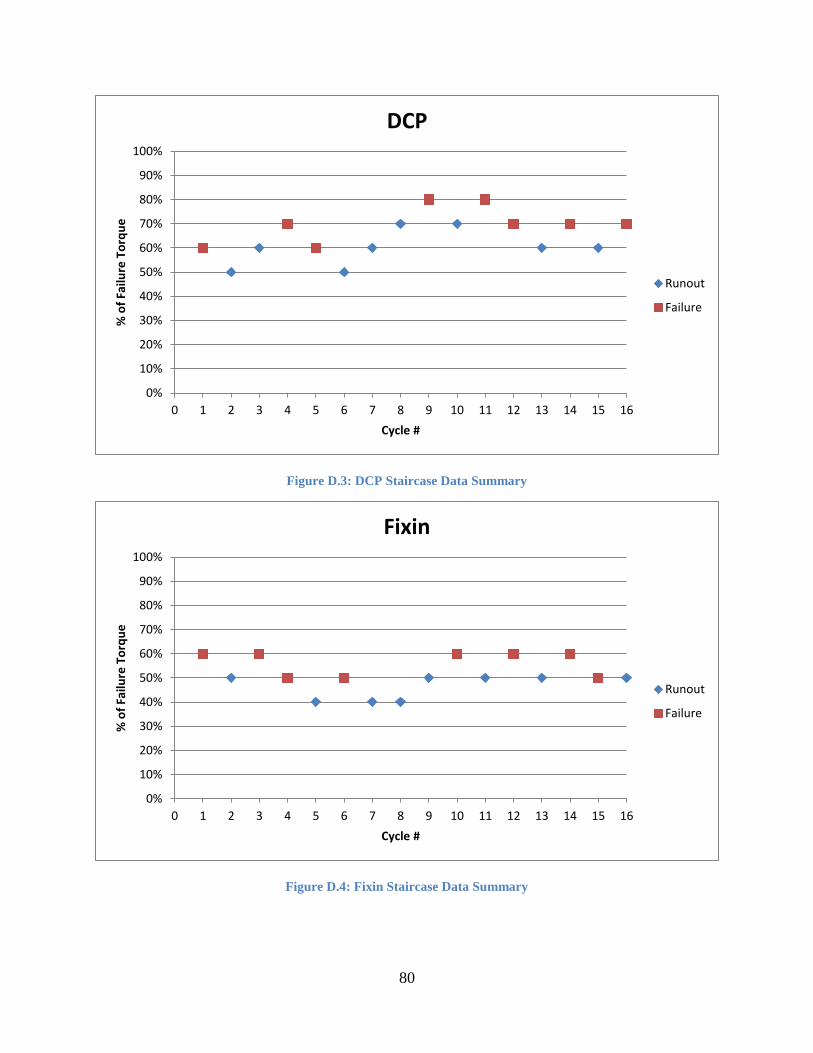
80
Figure D.3: DCP Staircase Data Summary
Figure D.4: Fixin Staircase Data Summary
0%
10%
20%
30%
40%
50%
60%
70%
80%
90%
100%
0 1 2 3 4 5 6 7 8 9 10 11 12 13 14 15 16
% o
f Fa
ilure
To
rqu
e
Cycle #
DCP
Runout
Failure
0%
10%
20%
30%
40%
50%
60%
70%
80%
90%
100%
0 1 2 3 4 5 6 7 8 9 10 11 12 13 14 15 16
% o
f Fa
ilure
To
rqu
e
Cycle #
Fixin
Runout
Failure
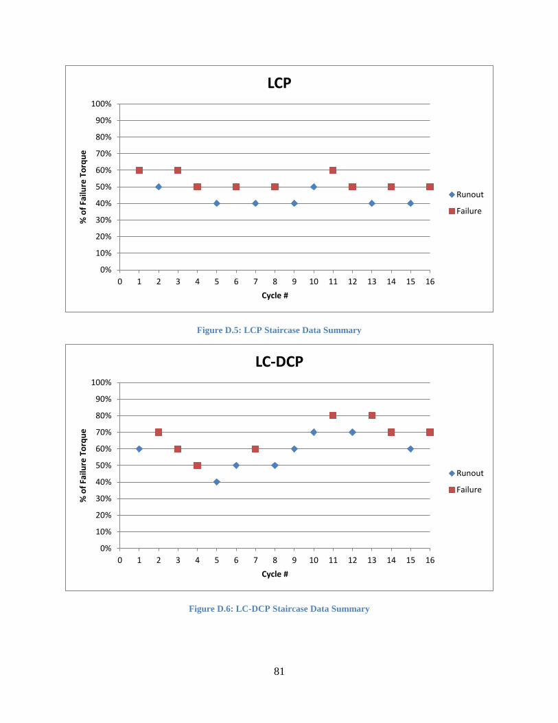
81
Figure D.5: LCP Staircase Data Summary
Figure D.6: LC-DCP Staircase Data Summary
0%
10%
20%
30%
40%
50%
60%
70%
80%
90%
100%
0 1 2 3 4 5 6 7 8 9 10 11 12 13 14 15 16
% o
f Fa
ilure
To
rqu
e
Cycle #
LCP
Runout
Failure
0%
10%
20%
30%
40%
50%
60%
70%
80%
90%
100%
0 1 2 3 4 5 6 7 8 9 10 11 12 13 14 15 16
% o
f Fa
ilure
To
rqu
e
Cycle #
LC-DCP
Runout
Failure

82
Figure D.7: SOP Staircase Data Summary
0
0.1
0.2
0.3
0.4
0.5
0.6
0.7
0.8
0.9
1
0 1 2 3 4 5 6 7 8 9 10 11 12 13 14 15 16
% o
f Fa
ilure
To
rqu
e
Cycle #
SOP
Runout
Failure

83
Appendix E: Cyclic Torsion Total Angular Rotation and Failure Modes
Angular rotation, per sample, in degrees, at various cycle points.
Failure Mode Key: Runout = No failure , F Progressive = Progressive, noncatastrophic failure across entire cycle ,
F Acute = Catastrophic failure prior to end of cycle
Cycle 1 ALPS10 (60%) ALPS11 (60%) DCP (60%) Fixin (60%) LCP (60%) LC-DCP (60%) SOP (60%)
1000 15.99 17.28 12.16 13.83 12.46 9.94 13.94
5000 17.94 18.36 12.83 14.30 14.93 10.03 14.64
10000 19.50 19.50 15.52 14.93 18.23 10.25 19.91
15000 22.29 20.42 N/A 18.32 N/A 10.40 N/A
Mode: F Progressive Runout F Acute F Acute F Acute Runout F Acute
Rotation: 39% 18% 28% 32% 46% 5% 43%
Cycle 2 ALPS10 (50%) ALPS11 (70%) DCP (50%) Fixin (54%) LCP (54%) LC-DCP (70%) SOP (50%)
1000 11.65 20.59 9.39 12.00 11.61 12.79 11.83
5000 12.29 23.34 9.50 12.08 11.93 12.78 12.05
10000 12.52 26.16 10.00 12.08 12.33 13.32 14.77
15000 12.65 N/A 10.02 12.13 13.06 15.27 N/A
Mode: Runout F Acute Runout Runout Runout F Acute F Acute
Rotation: 9% 27% 7% 1% 12% 19% 25%
Cycle 3 ALPS10 (60%) ALPS11 (60%) DCP (60%) Fixin (60%) LCP (60%) LC-DCP (60%) SOP (40%)
1000 15.37 15.89 10.92 13.55 13.85 10.99 9.07
5000 16.38 -88.98 11.25 13.82 15.22 11.41 9.09
10000 16.84 N/A 10.87 -26.8 18.09 13.27 9.15
15000 17.35 N/A 9.94 N/A N/A 13.44 10.08
Mode: Runout F Acute Runout F Acute F Acute F Acute Runout
Rotation: 13% 660% 9% 298% 31% 22% 11%
Cycle 4 ALPS10 (70%) ALPS11 (50%) DCP (70%) Fixin (50%) LCP (50%) LC-DCP (50%) SOP (50%)
1000 17.75 11.81 13.31 10.59 11.15 7.85 11.94
5000 19.92 12.49 13.58 10.62 11.38 8.03 12.44
10000 21.16 13.22 14.02 12.23 14.21 8.85 14.34
15000 21.53 14.32 16.67 -21.29 17.76 9.20 38.88
Mode: Runout Runout F Progressive F Acute F Acute F Acute F Acute
Rotation: 21% 21% 25% 301% 59% 17% 226%
Cycle 5 ALPS10 (80%) ALPS11 (60%) DCP (60%) Fixin (40%) LCP (40%) LC-DCP (40%) SOP (40%)
1000 24.39 15.81 11.1 8.56 9.11 7.48 8.89
5000 26.66 20.76 11.48 8.65 9.17 7.48 8.89
10000 28.13 N/A 11.74 8.69 9.22 7.47 8.94
15000 29.11 N/A 14.62 8.66 9.24 7.46 9.04
Mode: F Acute F Acute F Progressive Runout Runout Runout Runout
Rotation: 19% 31% 32% 1% 1% 0% 2%
Cycle 6 ALPS10 (70%) ALPS11 (50%) DCP (50%) Fixin (50%) LCP (50%) LC-DCP (50%) SOP (50%)
1000 19.41 13.91 8.29 11.05 10.61 8.56 11.09
5000 20.95 14.07 8.21 11.23 11.13 8.66 12.14
10000 21.53 14.34 8.2 15.8 12.67 8.68 18.23
15000 21.92 14.65 8.26 N/A N/A 8.73 N/A
Mode: Runout Runout Runout F Acute F Acute Runout F Acute
Rotation: 13% 5% 0% 43% 19% 2% 64%
Cycle 7 ALPS10 (80%) ALPS11 (60%) DCP (60%) Fixin (40%) LCP (40%) LC-DCP (60%) SOP (40%)
1000 20.82 14.58 12.05 8.42 9.1 11.96 8.85
5000 22.5 15.03 12.17 8.12 9.13 12.31 8.88
10000 23.31 15.23 12.36 8.48 9.33 15.35 8.88
15000 24.44 15.41 12.46 8.48 9.6 15.59 8.94
Mode: Runout Runout Runout Runout Runout F Acute Runout
Rotation: 17% 6% 3% 1% 5% 30% 1%
Cycle 8 ALPS10 (90%) ALPS11 (70%) DCP (70%) Fixin (50%) LCP (50%) LC-DCP (50%) SOP (50%)
1000 26.08 24.82 12.91 11.2 9.96 8.2 11.56
5000 30.29 34.05 12.97 11.21 10.87 8.17 11.7
10000 43.77 N/A 13.6 11.23 11.32 8.2 11.99
15000 N/A N/A 14.04 11.48 12.86 8.2 19.06
Mode: F Acute F Acute Runout Runout F Acute Runout F Acute
Rotation: 68% 37% 9% 3% 29% 0% 65%
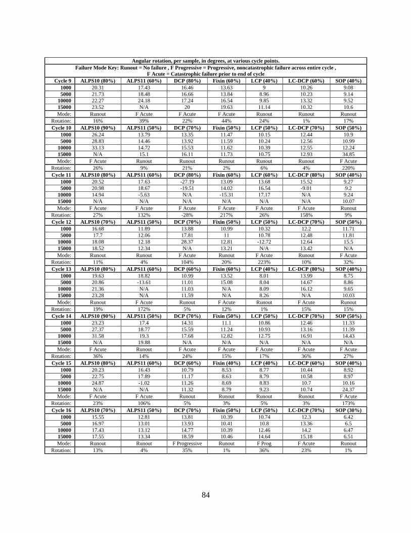
84
Angular rotation, per sample, in degrees, at various cycle points.
Failure Mode Key: Runout = No failure , F Progressive = Progressive, noncatastrophic failure across entire cycle ,
F Acute = Catastrophic failure prior to end of cycle
Cycle 9 ALPS10 (80%) ALPS11 (60%) DCP (80%) Fixin (60%) LCP (40%) LC-DCP (60%) SOP (40%)
1000 20.31 17.43 16.46 13.63 9 10.26 9.08
5000 21.73 18.48 16.66 13.84 8.96 10.23 9.14
10000 22.27 24.18 17.24 16.54 9.85 13.32 9.52
15000 23.52 N/A 20 19.63 11.14 10.32 10.6
Mode: Runout F Acute F Acute F Acute Runout Runout Runout
Rotation: 16% 39% 22% 44% 24% 1% 17%
Cycle 10 ALPS10 (90%) ALPS11 (50%) DCP (70%) Fixin (50%) LCP (50%) LC-DCP (70%) SOP (50%)
1000 26.24 13.79 13.35 11.47 10.15 12.44 10.9
5000 28.83 14.46 13.92 11.59 10.24 12.56 10.99
10000 33.13 14.72 15.53 11.62 10.39 12.55 12.24
15000 N/A 15.1 16.11 11.73 10.75 12.93 34.85
Mode: F Acute Runout Runout Runout Runout Runout F Acute
Rotation: 26% 9% 21% 2% 6% 4% 220%
Cycle 11 ALPS10 (80%) ALPS11 (60%) DCP (80%) Fixin (60%) LCP (60%) LC-DCP (80%) SOP (40%)
1000 20.52 17.63 -27.19 13.09 13.68 15.52 9.27
5000 20.98 18.67 -19.51 14.02 16.54 -9.01 9.2
10000 14.94 -5.63 N/A -15.31 17.17 N/A 9.24
15000 N/A N/A N/A N/A N/A N/A 10.07
Mode: F Acute F Acute F Acute F Acute F Acute F Acute Runout
Rotation: 27% 132% -28% 217% 26% 158% 9%
Cycle 12 ALPS10 (70%) ALPS11 (50%) DCP (70%) Fixin (50%) LCP (50%) LC-DCP (70%) SOP (50%)
1000 16.68 11.89 13.88 10.99 10.32 12.2 11.71
5000 17.7 12.06 17.81 11 10.78 12.48 11.81
10000 18.08 12.18 28.37 12.81 -12.72 12.64 15.5
15000 18.52 12.34 N/A 13.21 N/A 13.42 N/A
Mode: Runout Runout F Acute Runout F Acute Runout F Acute
Rotation: 11% 4% 104% 20% 223% 10% 32%
Cycle 13 ALPS10 (80%) ALPS11 (60%) DCP (60%) Fixin (60%) LCP (40%) LC-DCP (80%) SOP (40%)
1000 19.63 18.82 10.99 13.52 8.01 13.99 8.75
5000 20.86 -13.61 11.01 15.08 8.04 14.67 8.86
10000 21.36 N/A 11.03 N/A 8.09 16.12 9.65
15000 23.28 N/A 11.59 N/A 8.26 N/A 10.03
Mode: Runout F Acute Runout F Acute Runout F Acute Runout
Rotation: 19% 172% 5% 12% 1% 15% 15%
Cycle 14 ALPS10 (90%) ALPS11 (50%) DCP (70%) Fixin (50%) LCP (50%) LC-DCP (70%) SOP (50%)
1000 23.23 17.4 14.31 11.1 10.86 12.46 11.33
5000 27.37 18.77 15.59 11.24 10.93 13.16 11.39
10000 31.58 19.3 17.68 12.82 12.75 16.91 14.43
15000 N/A 19.88 N/A N/A N/A N/A N/A
Mode: F Acute Runout F Acute F Acute F Acute F Acute F Acute
Rotation: 36% 14% 24% 15% 17% 36% 27%
Cycle 15 ALPS10 (80%) ALPS11 (60%) DCP (60%) Fixin (40%) LCP (40%) LC-DCP (60%) SOP (40%)
1000 20.23 16.43 10.79 8.53 8.77 10.44 8.92
5000 22.75 17.89 11.17 8.63 8.79 10.58 8.97
10000 24.87 -1.02 11.26 8.69 8.83 10.7 10.16
15000 N/A N/A 11.32 8.79 9.23 10.74 24.37
Mode: F Acute F Acute Runout Runout Runout Runout F Acute
Rotation: 23% 106% 5% 3% 5% 3% 173%
Cycle 16 ALPS10 (70%) ALPS11 (50%) DCP (70%) Fixin (50%) LCP (50%) LC-DCP (70%) SOP (30%)
1000 15.55 12.81 13.81 10.39 10.74 12.3 6.42
5000 16.97 13.01 13.93 10.41 10.8 13.36 6.5
10000 17.43 13.12 14.77 10.39 12.46 14.2 6.47
15000 17.55 13.34 18.59 10.46 14.64 15.18 6.51
Mode: Runout Runout F Progressive Runout F Prog F Acute Runout
Rotation: 13% 4% 35% 1% 36% 23% 1%
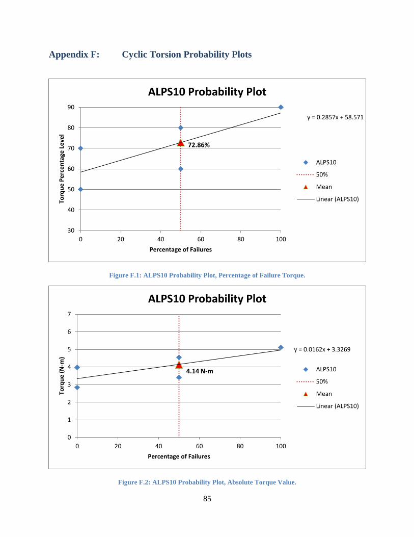
85
Appendix F: Cyclic Torsion Probability Plots
Figure F.1: ALPS10 Probability Plot, Percentage of Failure Torque.
Figure F.2: ALPS10 Probability Plot, Absolute Torque Value.
72.86%
y = 0.2857x + 58.571
30
40
50
60
70
80
90
0 20 40 60 80 100
Torq
ue
Pe
rce
nta
ge L
eve
l
Percentage of Failures
ALPS10 Probability Plot
ALPS10
50%
Mean
Linear (ALPS10)
4.14 N-m
y = 0.0162x + 3.3269
0
1
2
3
4
5
6
7
0 20 40 60 80 100
Torq
ue
(N
-m)
Percentage of Failures
ALPS10 Probability Plot
ALPS10
50%
Mean
Linear (ALPS10)
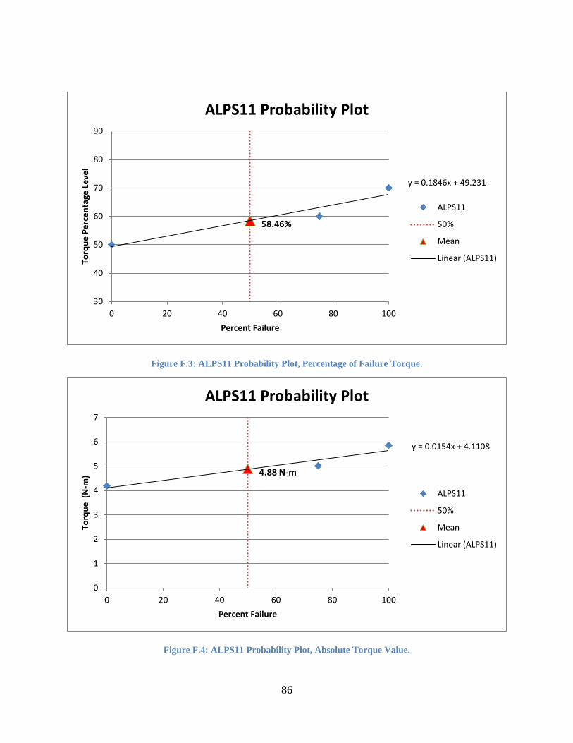
86
Figure F.3: ALPS11 Probability Plot, Percentage of Failure Torque.
Figure F.4: ALPS11 Probability Plot, Absolute Torque Value.
58.46%
y = 0.1846x + 49.231
30
40
50
60
70
80
90
0 20 40 60 80 100
Torq
ue
Pe
rce
nta
ge L
eve
l
Percent Failure
ALPS11 Probability Plot
ALPS11
50%
Mean
Linear (ALPS11)
4.88 N-m
y = 0.0154x + 4.1108
0
1
2
3
4
5
6
7
0 20 40 60 80 100
Torq
ue
(N
-m)
Percent Failure
ALPS11 Probability Plot
ALPS11
50%
Mean
Linear (ALPS11)
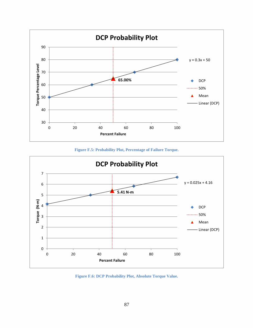
87
Figure F.5: Probability Plot, Percentage of Failure Torque.
Figure F.6: DCP Probability Plot, Absolute Torque Value.
65.00%
y = 0.3x + 50
30
40
50
60
70
80
90
0 20 40 60 80 100
Torq
ue
Pe
rce
nta
ge L
eve
l
Percent Failure
DCP Probability Plot
DCP
50%
Mean
Linear (DCP)
5.41 N-m
y = 0.025x + 4.16
0
1
2
3
4
5
6
7
0 20 40 60 80 100
Torq
ue
(N
-m)
Percent Failure
DCP Probability Plot
DCP
50%
Mean
Linear (DCP)

88
Figure F.7: Fixin Probability Plot, Percentage of Failure Torque.
Figure F.8: Fixin Probability Plot, Absolute Torque Value.
50.82%
y = 0.1959x + 41.02
30
40
50
60
70
80
90
0 20 40 60 80 100
Torq
ue
Pe
rce
nta
ge L
eve
l
Percent Failure
Fixin Probability Plot
Fixin
50%
Mean
Linear (Fixin)
3.45 N-m
y = 0.0133x + 2.7894
0
1
2
3
4
5
6
7
0 20 40 60 80 100
Torq
ue
(N
-m)
Percent Failure
Fixin Probability Plot
Fixin
50%
Mean
Linear (Fixin)

89
Figure F.9: LCP Probability Plot, Percentage of Failure Torque.
Figure F.10: LCP Probability Plot, Absolute Torque Value.
46.84%
y = 0.2279x + 35.442
30
40
50
60
70
80
90
0 20 40 60 80 100
Torq
ue
Pe
rce
nta
ge L
eve
l
Percent Failure
LCP Probability Plot
LCP
50%
Mean
Linear (LCP)
3.99 N-m
y = 0.0194x + 3.0232
0
1
2
3
4
5
6
7
0 20 40 60 80 100
Torq
ue
(N
-m)
Percent Failure
LCP Probability Plot
LCP
50%
Mean
Linear (LCP)

90
Figure F.11: LC-DCP Probability Plot, Percentage of Failure Torque.
Figure F.12: LC-DCP Probability Plot, Absolute Torque Value.
61.392
y = 0.418x + 40.492
30
40
50
60
70
80
90
0 20 40 60 80 100
Torq
ue
Pe
rce
nta
ge L
eve
l
Percent Failure
LC-DCP Probability Plot
LC-DCP
50%
Mean
Linear (LC-DCP)
4.65 N-m
y = 0.0317x + 3.0693
0
1
2
3
4
5
6
7
0 20 40 60 80 100
Torq
ue
(N
-m)
Percent Failure
LC-DCP Probability Plot
LC-DCP
50%
Mean
Linear (LC-DCP)

91
Figure F.13: SOP Probability Plot, Percentage of Failure Torque.
Figure F.14: SOP Probability Plot, Absolute Torque Value.
44.21%
y = 0.2211x + 33.157
30
40
50
60
70
80
90
0 20 40 60 80 100
Torq
ue
Pe
rce
nta
ge L
eve
l
Percent Failure
SOP Probability Plot
SOP
50%
Mean
Linear (SOP)
3.83 N-m
y = 0.0191x + 2.8714
0
1
2
3
4
5
6
7
0 20 40 60 80 100
Torq
ue
(N
-m)
Percent Failure
SOP Probability Plot
SOP
50%
Mean
Linear (SOP)

92
Appendix G: Dixon-Mood Calculations Table G.1: ALPS10 Dixon-Mood Calculations.
ALPS10 Range i n i*n i^2*n
90% 3 3 9 27
80% 2 3 6 12
70% 1 0 0 0 µ 76.43
60% 0 1 0 0 σDM 16.34
Total
A = 7 B = 15 C = 39 σSL 20.11
Table G.2: ALPS11 Dixon-Mood Calculations.
ALPS11 Range i n i*n i^2*n
70% 1 2 2 2 µ 57.50
60% 0 6 0 0 σDM 5.30
Total
A = 8 B = 2 C = 2 σSL 6.52
Table G.3: DCP Dixon-Mood Calculations.
DCP Range i n i*n i^2*n
80% 2 2 4 8
70% 1 4 4 4 µ 65.00
60% 0 2 0 0 σDM 8.57
Total
A = 8 B = 8 C = 12 σSL 10.55
Table G.4: Fixin Dixon-Mood Calculations.
Fixin Range i n i*n i^2*n
60% 1 5 5 5 µ 51.25
50% 0 3 0 0 σDM 5.30
Total
A = 8 B = 5 C = 5 σSL 6.52
Table G.5: LCP Dixon-Mood Calculations.
LCP Range i n i*n i^2*n
50% 1 2 2 2 µ 47.86
40% 0 5 0 0 σDM 5.30
Total
A = 7 B = 2 C = 2 σSL 6.52

93
Table G.6: LC-DCP Dixon-Mood Calculations.
LC-DCP Range i n i*n i^2*n
80% 3 2 6 18
70% 2 3 6 12
60% 1 2 2 2 µ 62.50
50% 0 1 0 0 σDM 15.66
Total
A = 8 B = 14 C = 32 σSL 19.27
Table G.7: SOP Dixon-Mood Calculations.
SOP Range i n i*n i^2*n
60% 3 0 0 0
50% 2 0 0 0
40% 1 6 6 6 µ 43.57
30% 0 1 0 0 σDM 5.30
Total
A = 7 B = 6 C = 6 σSL 6.52

94
Appendix H: Plot of Runout Torque vs. Rotational Displacement