Evaluation of Bureau of Land Management Protocols for Monitoring Stream Condition

Laura Y. Johnson

Thesis submitted to the Faculty of the Virginia Polytechnic Institute and State University in partial fulfillment of the requirements for the degree of

Master of Science

In Forestry

Dr. Stephen P. Prisley, Chair Dr. Paul Angermeier, Fisheries and Wildlife

Dr. W. Michael Aust, Forestry Dr. Conrad D. Heatwole, Biological Systems Engineering

Dr. Harold E. Burkhart, Department head

May 27, 2005 Blacksburg, VA

Keywords: Riparian areas, Geographic Information Systems, benthic macroinvertebrates, qualitative assessments, Livestock Grazing

Evaluation of Bureau of Land Management Protocols for Monitoring Stream Condition

Laura Y. Johnson

(ABSTRACT)

The goal of the Aquatic Indicators of Land Condition (AILC) project is to

develop analytical tools that integrate land condition information with stream condition

for improved watershed management within the United States Bureau of Land

Management (BLM). Based on the goal of the AILC, two objectives for this study were:

to determine the effect of four GIS-derived distance measurements on potential

relationships between common BLM landscape stressors (mining and grazing) and

changes in benthic macroinvertebrate community structure; and to assess the

effectiveness of individual questions on a commonly-used Bureau-wide qualitative

stream assessment protocol, the proper functioning condition (PFC) assessment.

The four GIS distance measurements assessed for biotic relevance included:

straight-line distance, slope distance, flow length, and travel time. No significant

relationships were found between the measured distance to stressor and

macroinvertebrate community structure. However, the hydrological relevance of flow

length and travel time are logically superior to straight-line and slope distance and should

be researched further.

Several individual questions in the PFC assessment had statistically significant

relationships with the final reach ratings and with field-measured characteristics. Two of

the checklist questions were significantly related to the number of cow droppings. This

may indicate a useful and efficient measure of stream degradation due to grazing. The

handling and use of the PFC assessment within the BLM needs further documentation

and examination for scientific viability, and the addition of quantitative measurements to

the PFC in determining restoration potential would be desirable.

2

Acknowledgements This degree paper is the result of cooperation and encouragement from many

individuals. I would like to thank the members of my committee: Dr. Stephen P. Prisley

(chair) for the opportunity to work on this project and lots of help; Dr. Paul Angermeier,

Dr. W. Michael Aust, and Dr. Conrad Heatwole, for their help, patience, and

encouragement.

I would also like to thank the Bureau of Land Management (BLM) for the

agency’s funding and support of this project. Many people within the BLM contributed

time, data, and assistance in this project. Jarrad Kosa, Richard Bulavinetz, Kevin Whalen,

Karl Stein, and Mark Vinson were instrumental in the development of the AILC project

and provided direction for the study. Additionally, BLM field and state office contacts

Melissa Cunningham, John Henderson, Craig Johnson, Charles Keeports, Patrick

Koelsch, James Kott, Todd Kuck, Tom Mendenhall, Jolie Pollet, Holly Schue, Anna

Smith, Cynthia Tait, and Craig Johnson, were invaluable in providing PFC checklists,

GIS data, and directing our summer field crews. Leon Pack at the BLM National Science

center in Denver provided grazing information from the RAS database.

Much of this research would not have been possible without the hard work of the

summer field crews, which included: Joshua Faulkner (2 summers), Adrian Harpold, and

Jennifer Moore. Aaron Bernard contributed greatly to the data processing involved in this

project, and also provided support and technical help. Finally, thank you to family and

friends for your support during this process.

iii

Table of Contents List of Tables ...................................................................................................................... v List of Figures .................................................................................................................... vi Chapter 1: Introduction ....................................................................................................... 1

1.1 Monitoring the Biotic Integrity of Water Resources ........................................... 1 1.2 Development of BLM stream monitoring............................................................. 3 1.3 BLM data resources................................................................................................ 6 1.4 Study objectives....................................................................................................... 7 Stream distance study ..................................................................................................... 7 PFC checklist study......................................................................................................... 7 Question A ...................................................................................................................... 8 Question B ...................................................................................................................... 8

Chapter 2: Literature Review.............................................................................................. 9 2.1 Riparian areas and their monitoring .................................................................... 9 2.2 The use of macroinvertebrates in stream monitoring ....................................... 11 2.3 Impacts of Mining and Livestock Grazing ......................................................... 16 2.4 Use of GIS and Spatial Scale................................................................................ 19

Chapter 3: Data and Methods ........................................................................................... 22 3.1 Base data ................................................................................................................ 22 3.2 Macroinvertebrate Data ....................................................................................... 25 3.3 Stressor Data ......................................................................................................... 26 3.4 Study area .............................................................................................................. 26 3.5 Methods for stream distance study ..................................................................... 31 3.6 Methods for PFC checklist study......................................................................... 53 PFC Question B ............................................................................................................ 54

Chapter 4: Results ............................................................................................................. 57 4.1 Objective 1 ............................................................................................................. 57 4.2 Objective 2A .......................................................................................................... 61 4.3 Objective 2B .......................................................................................................... 67

Chapter 5: Discussion ....................................................................................................... 72 5.1 Objective 1 ............................................................................................................. 72 5.2 Objective 2A .......................................................................................................... 74 5.3 Objective 2B .......................................................................................................... 77

Chapter 6: Conclusions ..................................................................................................... 82 6.1 Objective 1 ............................................................................................................. 82 6.2 Objective 2A .......................................................................................................... 82 6.3 Objective 2B .......................................................................................................... 83

Chapter 7: Literature Cited ............................................................................................... 85 Appendix A: PFC Assessment checksheet ....................................................................... 91 Appendix B: Stream sampling data sheet used by AILC ................................................. 93

iv

List of Tables

Table 1. Data types and sources used in the study............................................................ 23 Table 2. Characteristics of study areas chosen for the stream distance study. ................. 27 Table 3. District offices and participating field offices within each district..................... 30 Table 4. Comparison of distance calculation methods used in the stream distance study.

With increased model attributes and number of inputs comes increased potential error and decreased spatial certainty......................................................................... 31

Table 5. Calculation of Hydraulic radius, R, given a constant cross-sectional area for five common channel shapes. R = Area/Wetted Perimeter.............................................. 44

Table 6. Stream types and Manning’s n values used for the study(Ward and Trimble 2004). ........................................................................................................................ 45

Table 7. Wyoming GAP categories, cover types, and Manning’s n values assigned (Ward and Trimble 2004)..................................................................................................... 47

Table 8. Utah GAP categories, cover types, and assigned Manning’s n values.(Ward and Trimble 2004) ........................................................................................................... 48

Table 9. PFC questions with applicable measured site characteristics. ............................ 55 Table 10. Differences in mean and range of values for the macroinvertebrate metrics used

in the stream distance study. ..................................................................................... 59 Table 11. Comparison of mean EPT (Ephemoptera, Plectoptera, Trichoptera) abundances

between Omernik’s (1989) aquatic ecoregions using Tukey’s HSD (Significant probabilities are in bold). .......................................................................................... 60

Table 12. Wald statistic test results on individual questions in the ordinal logistic regression model.Significant probabilities (α = 0.05) are given in bold. Where degrees of freedom (DF) = 1, responses only consisted of “yes” and “no”; where DF = 2, responses included “yes”, “no” and “N/A”. ...................................................... 64

Table 13. Parameter estimates and Chi-Squared test results for individual questions for both the yes, no responses and the yes, N/A responses for each significant question from Table 12. Significant probabilities (α = 0.05) are given in bold. ..................... 65

Table 14. PCA results for PFC checklist study objective A. The first two axes account for 47.4% of the variance in samples, with diminishing percent variance explained for higher-level axes. ...................................................................................................... 65

Table 15. Question loadings (eigenvalues) in the PCA analysis. Question 2 had the highest loading of axis 2, question 13 has the largest loading of axis one, and question 12 has the smallest and only positive loading of axis one.......................... 66

Table 16. Comparison and results of PFC responses with field crew measured or observed characteristics. Significant probabilities are given in bold........................ 69

Table 17. Principal Components loadings of the PCA analysis of field-crew measured characteristics............................................................................................................ 71

v

List of Figures

Figure 1. Utah study areas. Note the area within Arizona, however, there are no sample points within Arizona................................................................................................ 28

Figure 2. Wyoming study area for stream distance study................................................. 29 Figure 3. Locations of participating BLM districts and reach locations for the checklist

question study. .......................................................................................................... 30 Figure 4. Straight-line distance for sample point ES-169 in Utah (triangle). The

delineated watershed is the watershed for sample point ES-169. The black line shows the path used to measure distance between the sample point and the stressor (circle), 2377 meters. ................................................................................................ 33

Figure 5. Flow distance for sample point ES-169 in Utah (triangle). Flow distance in meters was calculated using Raster Calculator, which resulted in a grid. The path of the flow distance from the stressor (circle) to the sample is shown by the black line, 2899 m. ..................................................................................................................... 35

Figure 6. Travel time for sample point ES-169. Travel time follows the same path as flow distance (black line) but also incorporates information about ground cover. The travel time from the stressor (circle) to the sample point (triangle) was 95 minutes.36

Figure 7. Selection of a DEM-generated Flow Netwotk (DEF-FN) for the Utah 1 subwatershed. Each DEM-FN was compared with the Digital Raster Graphic flow network (DRG-FN), the same as those delineated on USGS topographic maps. Note how the DEM-FN 800 is almost completely hidden by the DRG-FN, however, the other generated FN are not........................................................................................ 39

Figure 8. Types of flow partitioned for the travel time calculations. Channel flow (dark blue) includes channels similar in length to those delineated on a UGSG topographic map. Overland flow (light yellow) includes the area from the top of the ridge (shown by USGS topo quad in black) 100 meters down, following the flow path distance from the ridge top, which results in an irregular border. Shallow flow (light blue) includes the areas in between the overland and channel flows and can indicate ephemeral drains and areas of rill flow..................................................................... 40

Figure 9. Visual comparison of travel time zones using high R (hydraulic radius) -value of 0.68 (grid on the right) and low R-value of 0.60 (grid on the left). Grids were separated by 180-minute intervals of time to outlet in a subwatershed in Utah 1. ... 44

Figure 10. Partition calculator created using ArcObjects (ESRI 2002)............................ 50 Figure 11. Watershed velocity calculator programmed using ArcObjects (ESRI 2002).. 51 Figure 12. Distribution of macroinvertebrate samples among years for the 247 sites used

in the stream distance study. ..................................................................................... 53 Figure 13. Scatter plots comparing the various distances calculated from grazing stressor

centroids to sample points. Two outliers with travel times greater than 1000 minutes were excluded. .......................................................................................................... 58

Figure 14. Sample sites that occurred within grazing polygons were identified using a GIS. ........................................................................................................................... 61

Figure 15. Distribution of reaches among contributing BLM Field Offices. BAK = Baker, Oregon; COL = Colorado; COT = Cottonwood, Idaho; ELK = Elko, Nevada; JAR = Jarbidge, Idaho; PRI = Prineville, Oregon; and WYO = Wyoming, which includes three separate field offices.......................................................................... 62

vi

Figure 16. Number of study sites used in objective 2A with reach ratings of PFC, FAR, and NF....................................................................................................................... 63

Figure 17. Mosaic plot of the proportion of reaches in each reach rating category by field office. Mosaic plots are calculated by dividing the X axis (Field Office) by the proportions of samples in each category, and then dividing the Y axis (Reach Rating) by the estimated probability responses of each office, or category. The final mosaic plot represents the frequency of each combination of reach rating (Y) and office (X) in relationship to all other possible combinations by the proportional area of the cell. BAK = Baker, Oregon; COL = Colorado; COT = Cottonwood, Idaho; ELK = Elko, Nevada; JAR = Jarbidge, Idaho; PRI = Prineville, Oregon; and WYO = Wyoming, which includes three separate field offices. Note that the Elko field office had only FAR reaches, but also had the smallest sample size (n = 10). ................... 63

Figure 18. Euclidean distance biplot of the first two principal components, PC 1 (x-axis) and PC 2 (y-axis). Clusters of points are outlined and labeled by their reach rating. All unlabeled points had a reach rating of FAR, the most common reach rating. Each numbered point represents one site and each arrow represents one checklist question.................................................................................................................................... 67

Figure 19. Biplot of the principal components (PC 1 and PC 2) for the analysis of field crew observations and measurements. There were no clear clusters of points by reach rating. Each numbered point represents one site............................................. 70

Figure 20. Mosaic plot of the dependence of PFC rating on the response to question 5 (p > 0.10). The mosaic plot represents the frequency of each combination of reach rating (Y) and answer to question 5 (X) in relationship to all other possible combinations by the proportional area of the cell..................................................... 75

Figure 21. Distribution in years of difference between the field crew visit and PFC assessment for all sites used in objective 2B. ........................................................... 80

vii

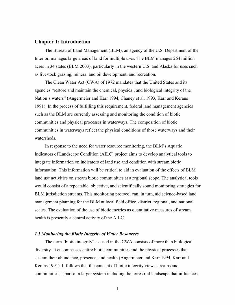
Chapter 1: Introduction The Bureau of Land Management (BLM), an agency of the U.S. Department of the

Interior, manages large areas of land for multiple uses. The BLM manages 264 million

acres in 34 states (BLM 2003), particularly in the western U.S. and Alaska for uses such

as livestock grazing, mineral and oil development, and recreation.

The Clean Water Act (CWA) of 1972 mandates that the United States and its

agencies “restore and maintain the chemical, physical, and biological integrity of the

Nation’s waters” (Angermeier and Karr 1994, Chaney et al. 1993, Karr and Kerans

1991). In the process of fulfilling this requirement, federal land management agencies

such as the BLM are currently assessing and monitoring the condition of biotic

communities and physical processes in waterways. The composition of biotic

communities in waterways reflect the physical conditions of those waterways and their

watersheds.

In response to the need for water resource monitoring, the BLM’s Aquatic

Indicators of Landscape Condition (AILC) project aims to develop analytical tools to

integrate information on indicators of land use and condition with stream biotic

information. This information will be critical to aid in evaluation of the effects of BLM

land use activities on stream biotic communities at a regional scope. The analytical tools

would consist of a repeatable, objective, and scientifically sound monitoring strategies for

BLM jurisdiction streams. This monitoring protocol can, in turn, aid science-based land

management planning for the BLM at local field office, district, regional, and national

scales. The evaluation of the use of biotic metrics as quantitative measures of stream

health is presently a central activity of the AILC.

1.1 Monitoring the Biotic Integrity of Water Resources

The term “biotic integrity” as used in the CWA consists of more than biological

diversity- it encompasses entire biotic communities and the physical processes that

sustain their abundance, presence, and health (Angermeier and Karr 1994, Karr and

Kerans 1991). It follows that the concept of biotic integrity views streams and

communities as part of a larger system including the terrestrial landscape that influences

1

them. Biotic integrity is “a quantitative expression of a number of known relationships

between human disturbance and the characteristics of the resident biota”(Karr and Kerans

1991). Therefore, measuring biotic integrity requires the establishment of reference

conditions and ongoing monitoring of stream and watershed conditions (Angermeier and

Karr 1994, Chessman 1999, Harrelson et al. 1994, Lundquist and Beatty 1999, Platts et

al. 1987). Reference conditions are physical and biotic conditions of stream reaches that

have had little to no human influence. The physical and biotic conditions of other, more

human-influenced, streams can be compared with the conditions of reference streams of a

similar location to assess the effects of human activity.

Monitoring is a system of observation and planning designed to track changes in

water resource conditions over time, particularly those changes influenced by

management (Platts et al. 1987). Variables monitored and measured in stream systems

may include physicochemical parameters (Meador and Goldstein 2003, Townsend et al.

1997), stream and floodplain morphology (Leopold 1994, Muhar and Jungwirth 1998),

riparian soils, riparian vegetation (Townsend et al. 1997, Wallace et al. 1997), catchment

land use and land cover (Bryce et al. 1999, Lammert and Allan 1999, Richards et al.

1997, Weigel et al. 2000), historical information on stream conditions and land use

(Harding et al. 1998), and biotic community composition (Delong and Brusven 1998,

Plafkin et al. 1989, Platts et al. 1987, Roth et al. 1996). These measurements of stream

resources can be taken using direct field observations or remote sensing. Remote sensing

utilizes aerial photos and digital spatial data to make measurements.

Water resource physical and biotic conditions can vary both temporally and

spatially (Poff and Ward 1990). Effective monitoring should therefore encompass a range

of spatial and temporal scales (Karr and Kerans 1991). Landscape influences on aquatic

systems may occur at multiple spatial scales and through multiple processes (Allan and

Johnson 1997). Water resource data can be organized at the watershed/ catchment level,

and the riparian/reach level. Watershed-level data incorporate all information about an

entire drainage area for a particular stream outlet point. Riparian-level data include

information about a particular stream reach and its surrounding zone of influence. Stream

reach-level data can also consist of the particular data collected at a point within the

reach, including detailed information about biotic communities, stream physicochemistry,

2

and stream morphology. Successful monitoring of stream conditions requires integration

of both levels of water resource data.

1.2 Development of BLM stream monitoring

In order to track the condition of streams under the BLM’s jurisdiction, a

monitoring protocol must be in place (Platts et al. 1987). The BLM has acquired stream

physical condition data for areas of its jurisdiction using the proper functioning condition

assessment protocol.

The term proper functioning condition (PFC) refers to the functionality of a stream

reach’s physical processes. Physical processes determine the hydrology, morphology, and

riparian vegetation of a particular stream segment or reach. PFC assessments are based on

the assumption that if physical processes are correctly functioning, a riparian area will be

consistently resilient after flooding (Prichard et al. 1998). Resiliency refers to a condition

of dynamic equilibrium, where the processes of aggradation (deposition) and degradation

(erosion) are offset by the channel’s physical properties, such as riparian rooting, channel

slope, and sediment size (DeBano and Schmidt 1989). According to the PFC assessment

manual (Prichard et al. 1998), if an area were not functioning properly, an imbalance of

aggradation and degradation and subsequent major channel alterations during flood

events would be expected.

The qualitative (judgment-based rather than measurement-based) PFC process is

widely used by the BLM. PFC is simple to implement, requires little to no quantitative

(measured) data or sample collection, and is designed for use across diverse BLM lands

(Prichard et al. 1998). PFC is a ranking procedure designed to help land managers rank

restoration potential of stream reaches. The procedure is to be completed by a team of

experts, who visit the site in question and fill out a standard lotic checklist to determine

the PFC ranking of the area (Appendix A). To complete a PFC assessment, after

answering the field sheet questions, observers place stream reaches in one of three

condition categories based on a qualitative assessment that focuses on the riparian area.

Questions about hydrologic characteristics, riparian vegetation, and erosional

characteristics of the site are addressed on the standard lotic checklist as yes/no answers

(Prichard et al. 1998). To determine the final ranking, the team is to consider their

3

answers to the check sheet questions and then determine an overall reach rating based on

their expert judgment. A rating of PFC or Proper Functioning Condition indicates that the

area is resilient to flooding. A rating of Functioning- At Risk (FAR) means that the area

has some important physical processes in place, but there is a high likelihood that a flood

would severely damage the area. Damage may consist of streambank damage, drastic

channel relocation, and accelerated erosion and deposition rates. A direction of change

(upward, downward, or trend not apparent) is associated with the FAR rating, referring to

the reach’s movement toward or away from PFC. A rating of Not Functioning (NF)

indicates that none of the physical processes assessed are functioning for the reach and

flood damage is usually already evident or damage is imminent with the next flood event

(Prichard et al. 1998).

For the remainder of this document, the entire PFC protocol or process will be

referred to as the “PFC assessment”. The questions on a checklist used during the PFC

assessment will be referred to as “checklist questions” and the checklist itself will be

called the “standard lotic checklist” or “checklist”, the final rating of a reach (PFC, FAR,

or NF) will be referred to as the “reach rating”, and a final rating of PFC for a specific

reach will be referred to as a “reach rating of PFC” to avoid confusion between the

overall name of the assessment and the ranking of a particular reach.

The PFC protocol is intended for use as an initial assessment of an area in order to

rank its restoration potential, not for use as a long- term monitoring tool or a watershed

analysis tool (Prichard et al. 1998, Pyke et al. 2002). Restoration is defined as the

“reestablishment of the structure and function of an ecosystem” (Williams et al. 1997). It

is unknown to what extent the PFC is used to rank restoration potential with follow-up

including restoration activities. Additionally, the current state of knowledge about the

PFC process and its scientific effectiveness is limited. Researchers are aware that the PFC

relies solely on professional opinion that is categorized as scientific procedure

(Stringham 2004).

Due to the widespread acceptance of the PFC process and its substitution for

quantitative science, although not the original intent of the authors (Prichard et al. 1998)

it would be prudent to scientifically assess its viability. The procedure’s widespread use

and acceptance in the BLM justifies its further scientific study.

4

In order to meet the AILC project’s objective of examining relationships between

stream conditions and land use, the land uses within BLM lands must be identified and

studied in addition to the PFC and instream biotic conditions. The BLM manages land for

many different uses, including recreation, livestock grazing, mining, and oil and gas

development. Management activities related to these land uses may include construction

of dams or water diversions, fencing, extermination of invasive and noxious weed

species, construction of roads, construction of oil and gas well heads, and construction of

mines and mine infrastructure. This study will focus on the impacts of grazing and

mining on macroinvertebrate communities.

To examine possible landscape factors affecting biotic integrity, a measure of biotic

integrity must be used. Biotic integrity can be quantified through the use of several types

of indices and metrics, which are discussed further in the literature review. These indices

can be calculated from collection of benthic macroinvertebrates or fish and quantifying

the community composition. The quantification method is determined by the index used.

Benthic macroinvertebrate communities are commonly-used indicators of watershed

health. Collection of macroinvertebrates is simple to implement, requires little specialized

equipment, and specimens can be kept in a laboratory for further analysis (Plafkin et al.

1989, Weber 1973). Macroinvertebrates are also plentiful in most streams and the wide

range of macroinvertebrate species can represent a gradient of pollution tolerances

(Rosenberg and Resh 1993).

The BLM manages 264 million acres of surface land, and is also responsible for

overseeing the mineral rights to 700 million acres of land in the U.S (BLM 2003). Mining

and mineral claims, along with oil and gas development, represented 92% of the revenue

generated by the BLM in 2003 (BLM 2003). Mining impacts on streams vary according

to the type of mining or mineral extraction, but can include direct pollution of heavy

metals, increased turbidity, and decreased pH (Grigorovich and Angermeier 2004).

The BLM also manages huge areas of range (livestock grazing areas). For example,

18,186 grazing permits and leases were issued in 2002 (BLM 2003). Streams are

frequently the only source of drinking water for livestock in rangelands, which can lead

to overuse and degradation of riparian areas (Platts 1991). The impact of rangeland

grazing on riparian areas is of increasing concern to many stakeholders (Clary and

5

Leininger 2000). The management of rangelands may affect stream quality both directly

and indirectly through alteration of water chemistry, soil properties, and vegetation cover

of riparian areas. Stream biotic and physical indicators assessed in this study may reflect

grazing and mining practices and help inform future management decisions.

1.3 BLM data resources

The BLM has access to many resources to aid in reaching the AILC project’s goals

of developing a sound stream monitoring system and providing objective information to

assist in making sound land management strategies at multiple levels. The PFC protocol,

macroinvertebrate data, land use information, spatial data, and Geographic Information

Systems (GIS) are all easily accessible to the BLM and will be integral in reaching the

goals of the AILC project.

The PFC process represents an excellent starting point for developing a

quantitative, objective, and repeatable monitoring protocol within BLM because of its

wide acceptance and implementation within the agency. Therefore, the strength of

correlation between PFC and landscape factors and instream conditions is an important

topic of study, and relevant to the goals of the AILC.

In addition, the BLM has access to entomologists who can identify and compile

macroinvertebrate data at the National Aquatic Monitoring Center (NAMC) in Logan,

Utah. The NAMC also trains field collection crews to collect macroinvertebrates with a

standardized sampling protocol.

The BLM also maintains several databases of management activities. The

Rangeland Assessment System (RAS) is one of these databases, used to catalog grazing

activity on all BLM lands (BLM 2003). Data on grazing allotment boundaries, vegetation

cover, land ownership, climate, mining development, and dam locations are also

available within the BLM or readily available through other federal agencies. Grazing

and mining location information are the most readily available landscape stressor data at

this time.

Furthermore, watershed and riparian area characteristics, including elevation,

stream order, road density, watershed area, and land cover, can all be derived remotely

from spatial datasets in a GIS. Using spatial datasets to derive these variables, rather than

field measurements, will reduce the amount of resources needed to generate information

6

for the AILC project. The correlation of PFC sampling points and macroinvertebrate

assemblages with these spatial variables will involve large amounts of spatial data at

varying spatial and temporal scales. GIS provides a system of data management, analysis,

and display of spatial data that will be of critical importance to the goals of the AILC.

This study will provide selected GIS analysis and data management for the AILC project.

1.4 Study objectives

Based on the goals of the AILC project and the resources available to the BLM, the

proposed research will include two related studies: a stream distance study and a PFC

checklist study.

Stream distance study

Potential relationships between landscape stressors and macroinvertebrate

community structure are of central importance to the goals of the AILC. If

macroinvertebrate community structure represents a monitoring structure that fulfills the

goals of the AILC, then the relationship between macroinvertebrate communities and

landscape activities will help guide management decisions. However, the location of a

stressor relative to a macroinvertebrate sampling site may affect the observed relationship

between the stressor and the biota at the sampling site.

The distance between stressor and sample point can be calculated in a variety of

different ways within a GIS. Which distance measure will result in the strongest

relationship between stressor and biotic sampling point? Does the intensity of the

stressor, i.e. the grazing pressure at a site, affect any relationship, quantified by distance,

between stressor and sample?

These questions were addressed using a GIS analysis of four distance

measurements for two stressors in Wyoming and Utah. The distance measures tested

included: straight-line (crow’s flight) distance, slope distance, flow length, and travel

time.

PFC checklist study

The study of the PFC assessment, its applicability to a wide range of western

BLM managed lands, and its overall viability will also be important to the goals of the

AILC in implementing an effective stream monitoring system. Study of the PFC

7

assessment will address two questions, outlined below. The analysis of the PFC process

will help to strengthen responses and the scientific relevance of the qualitative method. If

no relationships between checklist questions and final reach ratings, or between checklist

questions and field crew observations are found, then the use of the PFC process in the

BLM should be examined further.

Question A

Within the PFC assessment, do some questions contribute more than others to the

reach rating? Are some checklist questions redundant in determining the reach rating?

The answer to these questions may illustrate which parts of the PFC procedure, which

does not use any formal ranking or weighting measures, can be overlooked or simply not

considered by observers when assigning a final PFC ranking based on collective

responses to the 17 individual PFC questions.

Question B

Do standard lotic checklist responses correspond to measured field conditions? To

assess this question, measurements and observations recorded by a summer data

collection field crew (Appendix B) at sites with reach ratings previously assigned were

assumed to represent actual field conditions. Not all checklist questions have logical

corresponding field data, so a subset of the checklist questions was studied. Individual

PFC statement responses with stronger spatial correlations to instream characteristics

identify areas of the standard lotic checklist that effectively characterize measured field

conditions, while weak correlations of checklist responses and instream characteristics

may identify questions less effective in characterizing measured field conditions or a

need for further study. The response to each checklist question within the subset was

compared with the measurement (continuous) or observation (categorical) of the summer

field data.

8

Chapter 2: Literature Review Relevant literature in the study of riparian areas, macroinvertebrate sampling, land

use effects on riparian areas, and GIS analysis will be reviewed.

2.1 Riparian areas and their monitoring

The PFC assessment relies heavily on observable, moment-in-time riparian

properties to assess the “functioning condition” of a stream reach. The exact area that

determines a riparian zone, or area of influence around a stream, is subject to

interpretation. Chaney and others (1993) state that riparian areas are places next to bodies

of water where the vegetation is influenced by or dependent on the water body. Riparian

areas, particularly in the semiarid west, represent areas of rich resources for humans,

livestock, wildlife, and aquatic populations.

Riparian areas are often subject to continuous fluctuations in water levels, sediment

loads, and biotic communities and are therefore dynamic and complex systems (Naiman

et al. 2000). Snapshot-type monitoring of riparian areas is not sufficient to encompass the

wide range of fluctuations riparian areas undergo. Restoration activities should take into

account the highly dynamic nature of riparian areas (Ebersole and Liss 1997).

The term riparian area is ambiguous, although many researchers use a 100-m

straight-line buffer on either side of a stream as the standard area of riparian influence

(Pess et al. 2002, Richards et al. 1996). The problem with the use of straight-line buffers

around a stream is that they are determined by humans and not by the landscape. The

areas surrounding streams could differ greatly in topography or soil type, which could

affect the distribution of riparian vegetation, but the use of straight-line buffers does not

take these factors into account. However, the use of hydrologic travel time, or the time it

takes for precipitation to enter into a stream via the overland flow network, can be used to

delineate a riparian area of influence as well (Heatwole and Burcher 2003). Each point in

a watershed has a specific time to channel output associated with it for a given amount of

rainfall. These times could be generalized into zones (e.g. 30 minutes or less, 90 minutes

or less) and an appropriate zone chosen to represent the riparian area. An appropriate

travel time zone would closely follow the riparian and upland vegetation ecotone;

however, this research has not yet been done.

9

The determination of travel time may allow for better partitioning of the effects of

specific land uses on stream quality (Heatwole and Burcher 2003) at the landscape scale

than the use of riparian buffers. One disadvantage of this method compared to the use of

straight-line buffers is the time-consuming nature of calculations required for one riparian

area. However, GIS offers an excellent platform for calculation of these areas, and script

programs offer the possibility of full or partial automation of these processes.

In addition to the consideration of the area that makes up a riparian zone, the

method of communicating the physical and biotic properties of the riparian area is also of

importance. Indices are often used to categorize riparian monitoring data, and can be

calculated from measurements or qualitative observations. In North Carolina, scientists

conducted a pilot study in two sets of paired watersheds comparing the predictive power

of several qualitative indices of watershed health against an index of biotic integrity (IBI)

for fish (McQuaid and Norfleet 1999). Qualitative indices like the PFC are based on

several weight-of-evidence (McMahon et al. 2001) rather than measured observations.

The study found that all qualitative indices had a low correlation with IBI and suggested

that qualitative measures of watershed health have little utility and need further

examination. Although the PFC process is qualitative, the manual claims that the

questions are based on quantitative science (Prichard et al. 1998), and should therefore

have the potential for correlations with instream biotic condition.

The PFC manual describes for each of the 17 checklist questions supporting science

for the development of the question and any quantitative methods of evaluating the

question (Prichard et al. 1998). The reasoning behind the wording of most questions is

based on interpretation and assumption of conclusions of other studies. However, the

scientific relevance of a large portion of the questions is not clearly explained (questions

1, 2, 4, 7, 12, 14, 15, 16, 17, Appendix A) and assumes reader knowledge about literature

on the subject and provides no explicit scientific basis for the questions (Prichard et al.

1998). Several questions do have a clearly outlined scientific basis (questions 3, 5, 6, 8, 9,

10, 11, 13, Appendix A) with measurable characteristics, including Manning’s channel

roughness, Rosgen’s (1996) stream channel classification, empirical studies of channel

response to streamflow changes, Myers (1989) wetland plant classification, and Platts

and others’ (1987) method for determining streambank stability (Prichard et al. 1998).

10

However, the vague scientific background of many of the checklist questions further

warrants the scientific study of the PFC process.

2.2 The use of macroinvertebrates in stream monitoring

The relationship between PFC ratings and instream biotic conditions, as well as

riparian and watershed variables, is unknown. Studies of these correlations are integral to

the aforementioned goals of the AILC. Instream biotic conditions will be assessed for this

study using benthic macroinvertebrates. There are several advantages of using

macroinvertebrates over other biota, such as fish, including ease of collection, relatively

stationary nature, and the need for little specialized collection equipment (Plafkin et al.

1989, Weber 1973). There are also direct relationships between macroinvertebrate

abundance and fish production (Waters 1995). However, processing of macroinvertebrate

samples does require specialized knowledge and considerable time. Furthermore,

macroinvertebrate abundance fluctuates seasonally (Rosenberg and Resh 1993, Weber

1973). The plethora of available indices involving macroinvertebrates also suggests that

finding an appropriate measure of biotic integrity is difficult and variable (Rosenberg and

Resh 1993).

Macroinvertebrate community compositions can reflect changes over time. Because

of their stationary nature, many researchers believe that macroinvertebrates tend to reflect

changes in local or riparian conditions more than watershed-wide conditions (Lammert

and Allan 1999, Plafkin et al. 1989, Rosenberg and Resh 1993), although some authors

have disagreed (Weigel et al. 2000). Changes in macroinvertebrate communities may

reflect changes in substrate type, depth of stream, and velocity of streams (Weber 1973),

which may be directly or indirectly caused by natural variation or anthropogenic

influences, on local or watershed-wide scales. The partitioning of these wide ranges of

influences on macroinvertebrate communities will be discussed further.

There are several types of indices that can be generated using macroinvertebrates.

Diversity and biotic indices (Johnson et al. 1993) offer two distinct ways to compare

macroinvertebrate community structure with environmental factors. Useful indices

would show large differences between reference and disturbed sites at the onset of

11

disturbance, and diminishing difference as the disturbed site recovers over time (Stone

and Wallace 1998).

Diversity indices are based on the total number of individuals and total number of

taxa present (Norris and Georges 1993). Species abundance and species richness are

taken into account in the formulation of diversity indices. Diversity is assumed to be low

in environmentally stressed areas (Norris and Georges 1993). Common diversity indices

include Simpson’s index (Simpson 1949) and species per 1,000 individual organisms.

Biotic indices, based on known pollution tolerances, assign a ranking for each type

of organism observed or captured within a given area. The index is composed of these

individual species rankings, and sometimes will allow for physical and seasonal

fluctuations as well. Biotic indices are developed using assumptions about pollution type

and geography (Johnson et al. 1993).

The Hilsenhoff (1987) biotic index is one widely used biotic index. This index

ranks species by their organic pollution tolerance from 1 – 10 and also takes stream

current, temperature, and seasonal fluctuations into account (Hilsenhoff 1987). Because

this index is suited mainly for organic pollution impacts, it is suited for response to

grazing impacts (Grigorovich and Angermeier 2004). Another common biotic index is

the count of Ephemeroptera, Trichoptera, and Plecoptera (EPT) taxa. EPT taxa are

usually indicative of high-quality sites (Weigel et al. 2000), so the relative abundances of

these taxa are used to indicate the quality of a site. This index is simple to calculate, and

is suited for responding to impacts from development and direct, inorganic pollution such

as impacts from mining (Grigorovich and Angermeier 2004). The ratio of EPT to

Chironomidae taxa is thought to also include response to organic pollution impacts, such

as those from grazing (Grigorovich and Angermeier 2004). Many other biotic indices

exist as well (Rosenberg and Resh 1993) but these represent a small fraction of simple,

commonly-used, and available metrics for this study.

The relationship between macroinvertebrate community structure and riparian cover

has been widely studied, and is important when assessing land use influences on stream

condition. Riparian vegetation also represents a large portion of the variables assessed in

the PFC process (Prichard et al. 1998) and studying vegetation- related variables may

help illustrate any links between reach rating, land use, and instream biotic conditions.

12

The presence of riparian plants provides stability for streambanks and stream shading.

Percent vegetation cover has been related to land use (Townsend et al. 1997), particularly

grazing, development, and forestry.

Riparian vegetation provides organic matter in the form of leaves and woody

debris, which are important as food sources for specific groups of macroinvertebrates.

Riparian vegetation represents a significant portion of organic inputs to stream systems

(Kauffman and Kreuger 1984). Vegetation also provides shading and filtering properties

for streams (McEldowney et al. 2002). It follows that a decrease in riparian vegetation

would result in a loss of suitable habitat (increased temperature, increased turbidity) and

loss of food source for macroinvertebrates, which would be evident through changes in

the biotic community, for example, increased numbers of shredders. Scrimgeour and

Kendall (2003) found that the total biomass of invertebrates in grazed streams was

significantly affected by grazing practice.

Correlation between functional feeding groups and riparian vegetation is apparent

in some cases; however, this division of macroinvertebrate communities is not always

effective or necessary (Cummins 1974, Norris and Georges 1993). Macroinvertebrate

functional feeding groups can be indicators of land use and its effect on riparian

vegetation (Townsend et al. 1997). Shredders represent one functional feeding group with

direct connection to the amount and type of riparian vegetation. Shredders ingest the

largest particles of organic matter, mainly leaves, taking in about 40% of the matter for

internal processes and excreting the remaining 60%. Other feeding groups, such as the

collectors, feed on these particles (Cummins 1974). Reed and others (1994) found that

shredder biomass was higher in forested stream sites than in non-forested stream sites.

Similarly, Stout and others (1993) found that the response of shredders to disturbance

paralleled the response of the surrounding vegetation to disturbance.

Classifying the sources of variation in macroinvertebrate communities is

important to the goals of the AILC. Results of correlations between land use and physical

characteristics with macroinvertebrate biotic indices can be interpreted only by

understanding which community characteristics are a result of natural variation and

which are a result of land management practices and anthropogenic influences.

Classification of natural variance will be especially important due to the large regional

13

scope of the AILC project. There is a large body of literature on the partitioning of

variance in stream biota.

Poff and Ward (1990) identify several scales, or levels at which variation can be

classified. Spatial (regional to local), temporal (seasonal to geological), and ecological

(physiology and behavior to species migration) differences are all considerations in the

partitioning of variation in biotic communities (Poff and Ward 1990). Ecological scale

for this study will focus on macroinvertebrate assemblages, rather than individuals or

species migrations.

Classification methods for partitioning natural variance in benthic

macroinvertebrates are typically categorized using a large spatial scale (encompassing

large regions) or a small spatial scale (focusing on local variation). Large-scale

classifications use ecoregions, basins, or geology to account for natural variation in biotic

communities. There are several systems of ecoregionalization currently used, including

Major Land Resource Areas, the National Hierarchy of Ecological Units, and Level III

Ecosystems (McMahon et al. 2001). Ecoregions are large stratifications based on some

combination of any of the following factors: geology, land use, land cover, climate,

vegetation, and physiography (Omernik 1987). Hughes and others (1993) found that

ecoregions could not account for certain fauna and could not successfully predict fish

abundance. Ecoregions also have limited success in regionalizing biotic communities and

can be useful as a rough stratification framework for sampling design (Hawkins et al.

2000, Omernik and Bailey 1997) but not as a sole source for stratifying variation. Basins

are often difficult to use for classification, particularly in some geological areas (Omernik

and Bailey 1997).

Angermeier and others (2000) compared the effects of ecoregions and basins for on

variation in fish community composition. The authors found that a combination of

ecoregions and basins was more desirable than the use of just one of the two systems.

Van Sickle and Hughes (2000) studied the classification strengths of ecoregions and large

basins among other techniques. The authors concluded that large-scale geographic

partitioning by ecoregions or basin could account for only small amounts of natural

variation.

14

Some authors propose using geology alone as a large-scale stratification (Allan and

Johnson 1997). Harrellson and others (1994) also recommend classifying reference sites

based on underlying geomorphology. However, this is not likely to work as a stand-alone

large-scale classification for all geographic areas, as a study by Delong and Brusven

(1998) did not find that geologic patterns successfully partitioned macroinvertebrate

variation. This may be because the relative influence of geology on stream biota can vary

by geographic area.

Small-scale stratification considers smaller, more site-specific factors in

partitioning natural variation. Local characteristics are thought to be more effective

predictors of natural variation in stream macroinvertebrates (Hawkins et al. 2000).

Chessman (1999) proposes a method of classification that predicts species abundance

directly from a stream’s departure from local reference conditions: latitude, longitude,

temperature, elevation, and stream size. Stream substratum, stream flow rate, and

temperature have also been suggested as local stratification methods (Poff and Ward

1990).

Hawkins and Vinson (2000) state that due to the continuous nature of

environmental variation in streams, a classification system using small-scale

environmental gradients will be most effective in partitioning variation. The river

continuum concept (Vannote et al. 1980) also supports this theory. The river continuum

concept states that as a stream’s physical properties change from headwaters (the

uppermost part of a channel with flow significant enough to sustain macroinvertebrates)

to outlet, stream biotic properties should also change. This should result in a change in

the relative abundance of functional feeding groups. Shredders should dominate upper

reaches of the stream, where organic matter inputs are high, and the biotic community

composition should gradually shift towards collectors where the stream widens and

organic matter inputs are less important (Delong and Brusven 1998, Vannote et al. 1980).

In areas where the community abundances do not change longitudinally, this may

indicate a departure from reference conditions (Delong and Brusven 1998). Quantifying

these continua may prove more challenging than using large-scale stratification.

In addition to spatial variability, both benthic macroinvertebrates and stream

systems are subject to temporal variability. Over time, stream processes can change

15

naturally and benthic communities would change as well. The temporal regime of stream

systems is often ignored (Muhar and Jungwirth 1998) but is important to address. Land

use along a stream corridor also changes temporally (Allan and Johnson 1997). Karr and

Kerans (1991) state that monitoring of stream areas should occur at several temporal as

well as spatial scales. The effects of land use on macroinvertebrate communities and

their structure encompasses a large body of literature. The effect of livestock grazing and

mining as land uses of interest will be explored in this study.

2.3 Impacts of Mining and Livestock Grazing

Mining and livestock grazing on BLM lands are both economically important and

extensive current and historical land uses. Mining claims represent a large proportion of

BLM revenues (BLM 2003).

Impacts of mining and mineral extraction depend on the type and size of the mines.

Mining activities in the study area of interest included phosphate mining, hard rock

mining, and some extraction of construction materials (BLM 2003). However, there are

some generalized impacts of mining. Stream pollution by mine tailings (waste) can

increase heavy metal concentration in streams (Beasley and Kneale 2002, Marqués et al.

2003). Stream turbidity can also increase with increased erosion caused by surface

mining. Coal mining can lower stream pH dramatically in streams with low buffering

capacities (Jarvis and Younger 1997). In one study of several mining-related stream

characteristics as well as agriculture and physiography related characteristics, the biota

responded most strongly to the mining factors (García - Criado et al. 1999).

Concentrations of toxic metals, pH, and electrical conductivity are effective measures of

mining impacts on stream systems (Marqués et al. 2003).

Chaney and others (1993) state that grazing has more wide-reaching landscape

effects in the west than any other land use. Dividing grazing areas into allotments became

a common management practice in the 1960’s and is the most common organization of

range management used in the west today, particularly by the BLM (Platts 1991). Each

allotment may represent a different leasing ranch or use of a different grazing system.

Each allotment is further divided into any number of pastures, the number of which is

16

determined by the rancher’s needs, the number of livestock, and the grazing system in

use.

The amount of forage necessary to sustain one mature cow and her suckling calf for

thirty days is referred to as an animal unit month (AUM), where the cow and calf are

considered one animal unit. Other definitions of animal units also exist for other foraging

livestock. AUM’s are used to quantify the amount of forage resources needed, used, or

leased within an allotment or pasture.

Grazing systems refer to the rotation patterns of livestock within an area. There

are many types of grazing systems in use; continuous, rest-rotation, deferred, and high-

intensity short-duration systems are the most common systems in use on BLM lands in

the intermountain west. Holochek (1983) gives a through description of these patterns,

and other, lesser-used patterns. The following is a summary of Holochek’s descriptions.

Continuous grazing is the name given to any type of grazing using one pasture for

consecutive years. Continuous systems can cause some areas of pasture to be severely

overused, particularly riparian areas. In deferred rotation grazing, the rancher waits until

maturity has been reached on the most important feed grasses to rotate livestock into a

pasture. This system has proved advantageous in mountainous areas and areas where

plant availability and desirability are different. However, this system can also lead to

rapid degradation of riparian areas. Rest-rotation typically uses 4 pastures, where one

pasture is rested one full year every 4 years. Productivity of cattle may not be as high as

for other systems, however this system favors aesthetics and wildlife. High intensity short

duration grazing typically uses a ‘wagon wheel’ layout of pastures, where cattle are

moved between pastures at a high rate (4-6 weeks). Theoretically, high intensity short

duration would decrease infiltration of water due to the hoof impacts, and cause even use

of the entire allotment. In mountainous rangelands, this system can cause irreversible

damage to plants and soils. However, lowlands and areas with uniform plant palatability

and longer growing seasons may not be harmed by this system.

Both cattle and sheep graze BLM lands. Cattle grazing will be the focus of this

study, as they are more commonly grazed and their effects on stream habitats are heavily

researched. Additionally, there was no data or other evidence to suggest that sheep

grazing occurs on any of the study area lands. Cattle prefer riparian areas over upland

17

grazing areas, due to the increased water, thermal cover, high quality forage, and gentle

topography available in riparian areas (Clary and Leininger 2000, Kauffman and Kreuger

1984). Historically, overuse of rangeland riparian areas has been a problem (Chaney et al.

1993, Platts 1991), leaving the remaining functioning riparian areas with an increased

value to humans and wildlife (Kauffman and Kreuger 1984). This increased value of

rangeland riparian areas points to a need for informed, science-based management to

protect and restore remaining resources.

Grazing has many effects on water quality, both from upland and direct riparian

effects. Upland grazing areas, although not as heavily used as riparian areas, nevertheless

affect water quality. Upland pressures include trampling, an increase in soil bulk density

under intense grazing, the formation of trails which can lead to gully erosion, and

removal of vegetation which can lead to a decrease in infiltration (Trimble and Mendel

1995). This study took into account the effects of these upland (entire-watershed) impacts

through the flow-length and travel time distances.

There are many direct effects of cattle overuse on riparian communities, including

changes in stream morphology, water quality, wildlife habitat, and riparian vegetation

(Kauffman and Kreuger 1984). Grazing can cause compaction of soil in the riparian area,

which leads to decreased infiltration (Chaney et al. 1993). Erosion was found to increase

three to six times in grazed areas versus ungrazed areas in one study (Trimble 1994).

Cattle can also cause direct pollution through urine and manure, cause streambank

shearing by hooves, and influence the widening and shallowing of streams (Chaney et al.

1993, Clary and Leininger 2000, Waters 1995). Grazing can also lead to a loss of fish

habitat including smothering of spawning gravels and removal of riparian cover (Chaney

et al. 1993, Kauffman and Kreuger 1984, Waters 1995).

Overgrazing of riparian grasses can lead to the replacement of deep- rooted riparian

grasses with shallow-rooted species. This leads to increased bank width, decreased bank

stability, and increased turbidity (Clary and Leininger 2000, Manning et al. 1989, Platts

1991). In a study of grazing effects on sediment transport, stem density was found to be

one of the most important factors influencing sediment transport to streams, with higher

grass stem density reducing sediment transport. Grazing by cattle was found to reduce

stem density by 40% (McEldowney et al. 2002).

18

When examining potential relationships between land use and riparian condition, it

is important to acknowledge the dynamic nature of stream systems and the wide range of

natural and anthropogenic influences on these systems (Platts 1991). The natural

morphology and soil types of riparian areas and streams may render some areas more

sensitive to grazing pressure than others (Chaney et al. 1993). In modeling applications,

including the use of GIS, the diversity of rangeland types must be addressed. Rangelands

should be grouped according to their responses to precipitation and relationships among

physical characteristics for the development of valid models (Pierson et al. 2002).

2.4 Use of GIS and Spatial Scale

The conditions and processes of watersheds, riparian areas, and stream reaches

undoubtedly affect stream biota (Angermeier and Bailey 1992). A GIS has the ability to

store, process, display, and analyze spatial data quickly and efficiently, particularly at

large spatial scales. GIS can combine general scientific knowledge in visual form (maps)

with specific information in the form of a database (Longley et al. 2001). These

capabilities make GIS technology an effective tool in aquatic ecosystem management

(Angermeier and Bailey 1992).

Furthermore, GIS are equipped to handle multi-dimensional problems (Longley et

al. 2001). The multi-faceted nature of the interaction between land use and stream biota is

therefore well suited to GIS analysis. In addition, GIS can handle spatial distributions of

biotic characteristics, and can effectively model environmental processes (Longley et al.

2001), which will be vital to this study.

Watershed-scale variables such as catchment area, slope, stream gradient, road

density, vegetation cover, and similar relevant variables can be found by using GIS

algorithms and nationally available data. These types of variables have been used in a

variety of studies of impacts of land use on aquatic communities (Pess et al. 2002,

Richards et al. 1996, Roth et al. 1996, Sharma and Hillborn 2001). The ability of GIS to

determine variables remotely may save resources by eliminating the need for some field

measurements and calculations.

Distance from one geographic area to another is a common calculation that can be

made in GIS. Houlahan and Findlay (2004) found that different chemical and sediment

19

stressors created by deforestation significantly affected wetlands at different distances,

and the distances were fairly large, up to 4km. Additionally, there is scientific evidence

that not all methods of calculating distance are equally relevant (Yuan 2004b).

In the case of this study, the distance from a point stream sample to a point or

polygon landscape stressor is of interest. There are several ways that distance can be

calculated in GIS, each with an increasing level of required inputs and time.

The simplest way to calculate distance within a GIS is by using a spatial join. A

spatial join adds the attributes of one layer to another based on a spatial property, in this

case, distance. The distance from a feature in one layer to the closest feature in another

layer is recorded, along with the attributes of the closest feature (ESRI 2002).

Another method of calculating distance is by finding the change in elevation from

one feature to another. The net elevation change and the straight-line distance are used as

inputs to the Pythagorean theorem to find the distance between two points incorporating

the net elevation change. This is referred to as slope distance.

A third method of calculating distance to a hydrologic feature, such as a stream

sample point, can be calculated using the ArcGIS function flow length, which uses an

elevation dataset to calculate a flow path, rather than straight-line distance, based on

terrain. The flow length distance is the distance from the stressor to the nearest ephemeral

drain and the length of all ephemeral, intermittent, and perennial streams to the outlet

point. This function, when set to calculate downstream distance, will find the distance in

map units from each cell in the watershed of the sample point to the sample point (ESRI

2002).

GIS can also be used to determine hydrologic travel time based on time of

concentration (Heatwole and Burcher 2003). Extensive hydrology equations can be

calculated within GIS for display and analysis. This method requires the input of both

elevation and land cover data and the calculation of velocity for the watershed. The flow

length function is part of these calculations, although they are much more complex and

time-consuming than simply calculating flow length.

The specific limitations of the data inputs will be discussed in the review of data

and methods. With increasing modeling capability and increased inputs comes increased

potential error in the final distance measurement.The calculation of spatial attributes and

20

characteristics of watersheds must fit into the larger framework of the actual landscape

being studied, and the processes and extent of interest within that landscape. Therefore,

the determination of spatial scale is an important aspect to consider when designing a

study using GIS. Caution should be used when approaching problems from a large-scale

(regional extent) view. Regional data can be easily managed and processed in a GIS, but

study results may be extremely temporally variable (Wiley et al. 1997). Roth and others

(1996) did find that watershed (large) scale land use data analyzed using a GIS were

effective predictors of biotic indices and conditions of fish communities. A combination

approach of large-scale data and small-scale (local extent), temporally repeated (same

measurement made multiple years) data would also be appropriate (Wiley et al. 1997)

and would reduce variability due to temporal under-sampling. However, Lammert and

Allan (1999) found that a single-extent approach was often sufficient to identify

relationships between land use and biota, although they agreed with Wiley and others

(1997) that the nested approach would be ideal. Allan and Johnson (1997) also found that

changing spatial scale could result in different results, particularly with partitioning

variation. The authors also recommend using multiple spatial scales when approaching a

landscape level problem.

21

Chapter 3: Data and Methods Because this study will focus heavily on GIS analysis, several types of spatial and

attribute data will be used. Base physical data, macroinvertebrate data, and stressor data

will all be important in this study (Table 1). In addition to a review of data types, sources,

and accuracy, GIS and statistical methods for both studies will be explained.

3.1 Base data

Base GIS data for this project consisted of elevation, hydrography, land cover, and

land features. These data are used to derive other landform and watershed characteristics,

such as slope, stream order, flow accumulation, travel time, elevation, percent vegetative

cover, surface roughness, and other characteristics.

Elevation grids known as digital elevation models (DEMs) are available with

nationwide coverage through an online database. USGS topographic quad sheets partition

DEM coverage. The accuracy of DEM grids is categorized based on grid development

methods. Level 3 grids, the most accurate, are developed directly from hydrography and

hypsography topographic data. Level 3 DEMs are permitted a root mean square error

(RMSE; similar to standard deviation), of one-third of the topographic contour interval

(USGS 2002). Level 2 grids are the middle accuracy level, and are produced by

smoothing or filtering of older grids. Some hydrographic and hypsographic data are used

to increase accuracy of these grids. The maxium permitted RMSE for Level 2 grids is

one-half the topographic contour interval (USGS 2002). DEM data for the study area

selected are all level 3 DEM data (USGS 2002).

High-resolution DEM grids are usually 10 meters or 30 meters [USGS makes some

DEM grids with much lower resolution, like 1 km or 100 m]. Although the higher (10-m)

resolution would be more desirable, the accuracy level of data in the area should prove

more important than resolution level in deriving accurate measurements. In one study,

10-m Level 3 DEMs were found to be superior, particularly to the 30-m Level 1 DEMs,

in several categories of analysis. This was due more to the drainage enforcement

(enforced consistency between elevation-derived flow paths and hydrology) than the

increased resolution in the opinion of the authors (Clarke and Burnett 2003). Ten-meter

22

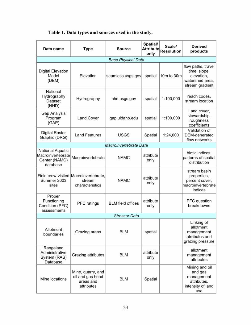
Table 1. Data types and sources used in the study.

Data name Type Source Spatial/

Attribute only

Scale/ Resolution

Derived products

Base Physical Data

Digital Elevation Model (DEM)

Elevation seamless.usgs.gov spatial 10m to 30m

flow paths, travel time, slope, elevation,

watershed area, stream gradient

National Hydrography

Dataset (NHD)

Hydrography nhd.usgs.gov spatial 1:100,000 reach codes, stream location

Gap Analysis Program (GAP)

Land Cover gap.uidaho.edu spatial 1:100,000

Land cover, stewardship, roughness coefficients

Digital Raster Graphic (DRG) Land Features USGS Spatial 1:24,000

Validation of DEM-generated flow networks

Macroinvertebrate Data National Aquatic

Macroinvertebrate Center (NAMC)

database

Macroinvertebrate NAMC attribute only

biotic indices, patterns of spatial

distribution

Field crew-visited Summer 2003

sites

Macroinvertebrate, stream

characteristics NAMC attribute

only

stream basin properties,

percent cover, macroinvertebrate

indices Proper

Functioning Condition (PFC)

assessments

PFC ratings BLM field offices attribute only PFC question

breakdowns

Stressor Data

Allotment boundaries Grazing areas BLM spatial

Linking of allotment

management atrributes and

grazing pressureRangeland

Administrative System (RAS)

Database

Grazing attributes BLM attribute only

allotment management

attributes

Mine locations

Mine, quarry, and oil and gas head

areas and attributes

BLM Spatial

Mining and oil and gas

management attributes,

intensity of land use

23

data were used for this study due to the available coverage in the western United

States. All DEM grids in the study area are 1/3 arc second (10-m) coverage (USGS

2002).

Digital elevation models can be used to derive watershed areas, flow networks,

watershed travel time, and other hydrologic and terrain variables in a GIS (Jenson and

Domingue 1988, Morris and Heerdegen 1988). It is important to note that any digital data

source will have inherent error in accordance with its source data and the technique used

to generate the data product. DEM elevations may not match field collected elevation

data, but when applied at a larger spatial scale, DEM derivatives can useful. There are

procedures and algorithms to reduce some of the error in DEM-derived flow networks

(Turcotte et al. 2001). A seamless version of DEM data is available through the National

Elevation Dataset (NED), which will be useful in study areas spanning more than one

topographic quadrangle map.

Hydrography data, including stream reach data and Hydrologic Unit Code (HUC)

boundaries are available through the National Hydrography Dataset (NHD), which is also

available online with nationwide coverage. Stream reach data for the NHD originates

from digital line graphs and EPA reach files (USGS 2000). The NHD contains streams,

bodies of water, coastlines, and wetlands in some areas. The NHD contains geocoded

reach data reach numbers as well as common stream names. Each stream reach has a

unique 14-digit permanent, non-transferable numeric identifier code, with the first 8

digits being the HUC code that the stream falls in, and the last 6 digits being the reach

code (USGS 2000). Producers of the NHD intend that these reach codes will be used to

identify and link information to stream reaches in a uniform manner. In addition to the

reach code, each reach also has a 10-digit common identifier code. The NHD also has

flow relationships and stream levels (the reverse of stream order, with the largest rivers

having the lowest level number) encoded (USGS 2000).

Land cover for areas in the stream distance study was determined through another

nationally available source, the gap analysis program (GAP). GAP data are available

online, free of charge, through the USGS. The GAP aims to provide vegetation and

stewardship mapping, in addition to species mapping, on a state-by-state basis (Jennings

24

and Scott 1997). Maps are produced at a 1:100,000 scale and are updated at regular

intervals, the length of which depends on the state.

Land features for areas in the stream distance study were needed to assess the

validity of DEM-generated flow networks. Digital raster graphics (DRG) are rasterized

USGS topographic maps, which show land features and topography at a 1:24000 scale.

DRG were used to determine flow networks mapped on USGS topographic quads for

selected study areas.

3.2 Macroinvertebrate Data

Macroinvertebrate point sampling data and biotic indices for specific sites were

available from the National Aquatic Monitoring Center (NAMC) in Logan, Utah. This

dataset provided the sampling points used in the stream distance study. A large (15,000

record) database of stream sample points covers many areas in the western U.S. The

dataset includes the sampling type (qualitative, quantitative), habitat type (coarse

particulate organic matter, riffle, multiple), total individuals counted, total taxa counted,

number of unique families, the number of unique genera, the number of unique

Ephemeroptera, Trichoptera, and Plecoptera genera. It can also include the calculated

Hilsenhoff (1987) biotic index, calculated Shannon’s diversity index, latitude and

longitude of the sample point, the water body type (stream, lake) and the organization or

individual who took the sample (Vinson 2003), it can also include many other calculated

metrics.

A field crew, referred to as the “summer field crew”, also sampled 79 sites with

previously assigned reach ratings in summer of 2003 and 84 sites in the summer of 2004.

Macroinvertebrate data were collected for both qualitative and quantitative assessments

and the NAMC processed these samples. Additionally, measurements of stream width,

percent overhead vegetative stream cover, stream substrate, flow rate, and temperature

were taken at each site, along with observations of land use at each stream site (Appendix

B). The NAMC catalogs the macroinvertebrate data into a database. The site

measurements that correspond with PFC statements were used in this study, which will

be discussed further.

25

PFC assessment sheets were acquired from BLM field offices for the points

sampled in summer 2003 and 2004. These ratings will provide the necessary individual

PFC responses as well as the overall ratings for each of these points. These PFC sheets

were entered into a Microsoft Access database and georeferenced to the summer data

points, along with the physical site data from the sampling field sheets.

3.3 Stressor Data

Specific allotment data were available through a large online BLM-managed

database, the Rangeland Administration System (RAS). RAS maintains information on

permitted rangelands for BLM in several states, including all of the states within the

Interior Columbia Basin (ICB). RAS contains information sorted by allotment on

permittees, grazing management, and grazing intensities. RAS data can be easily

associated with spatially linked grazing allotments using GIS. Digitized allotment

boundaries are available for some areas within individual BLM field offices.

Individual BLM field offices catalog mines, quarries, and oil and gas wells. There

is normally attribute data associated with these locations. Each field office records

varying degrees of detail about these stressors, however, so only location of the mines

were used for consistency within the study.

3.4 Study area

An appropriate study area for the stream distance study needed to fulfill several

characteristics. The area had to contain numerous sampling sites; contain areas of low

land use intensity; encompass a large geographic area in keeping with the desired

outcomes of the AILC; contain a large amount of BLM managed land; have grazing and

mining development as predominant land uses; and have spatial data readily available.

The selection of a study area was approached in three narrowing sets of criteria: available

land use data, differences in topographic relief and climate, and sufficient numbers of

existing macroinvertebrate sample plots and BLM managed land.

Areas within the AILC major study areas (northwest Wyoming, north central Idaho,

south central Utah, and northeast Oregon) that had readily available land use data

(grazing and mining) included only Utah and Wyoming. This strictly limited the further

26

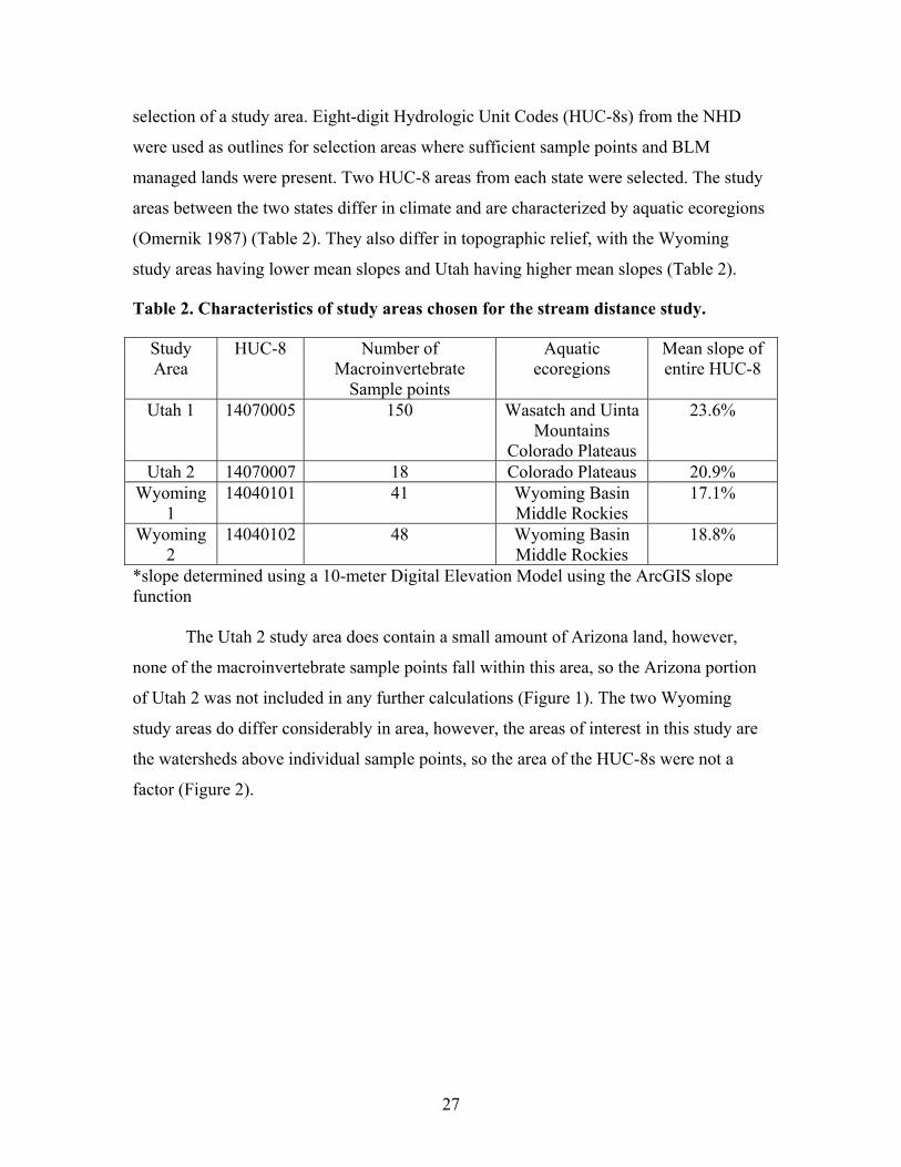
selection of a study area. Eight-digit Hydrologic Unit Codes (HUC-8s) from the NHD

were used as outlines for selection areas where sufficient sample points and BLM

managed lands were present. Two HUC-8 areas from each state were selected. The study

areas between the two states differ in climate and are characterized by aquatic ecoregions

(Omernik 1987) (Table 2). They also differ in topographic relief, with the Wyoming

study areas having lower mean slopes and Utah having higher mean slopes (Table 2).

Table 2. Characteristics of study areas chosen for the stream distance study.

Study Area

HUC-8 Number of Macroinvertebrate

Sample points

Aquatic ecoregions

Mean slope of entire HUC-8

Utah 1 14070005 150 Wasatch and Uinta Mountains

Colorado Plateaus

23.6%

Utah 2 14070007 18 Colorado Plateaus 20.9% Wyoming

1 14040101 41 Wyoming Basin

Middle Rockies 17.1%

Wyoming 2

14040102 48 Wyoming Basin Middle Rockies

18.8%

*slope determined using a 10-meter Digital Elevation Model using the ArcGIS slope function

The Utah 2 study area does contain a small amount of Arizona land, however,

none of the macroinvertebrate sample points fall within this area, so the Arizona portion

of Utah 2 was not included in any further calculations (Figure 1). The two Wyoming

study areas do differ considerably in area, however, the areas of interest in this study are

the watersheds above individual sample points, so the area of the HUC-8s were not a

factor (Figure 2).

27

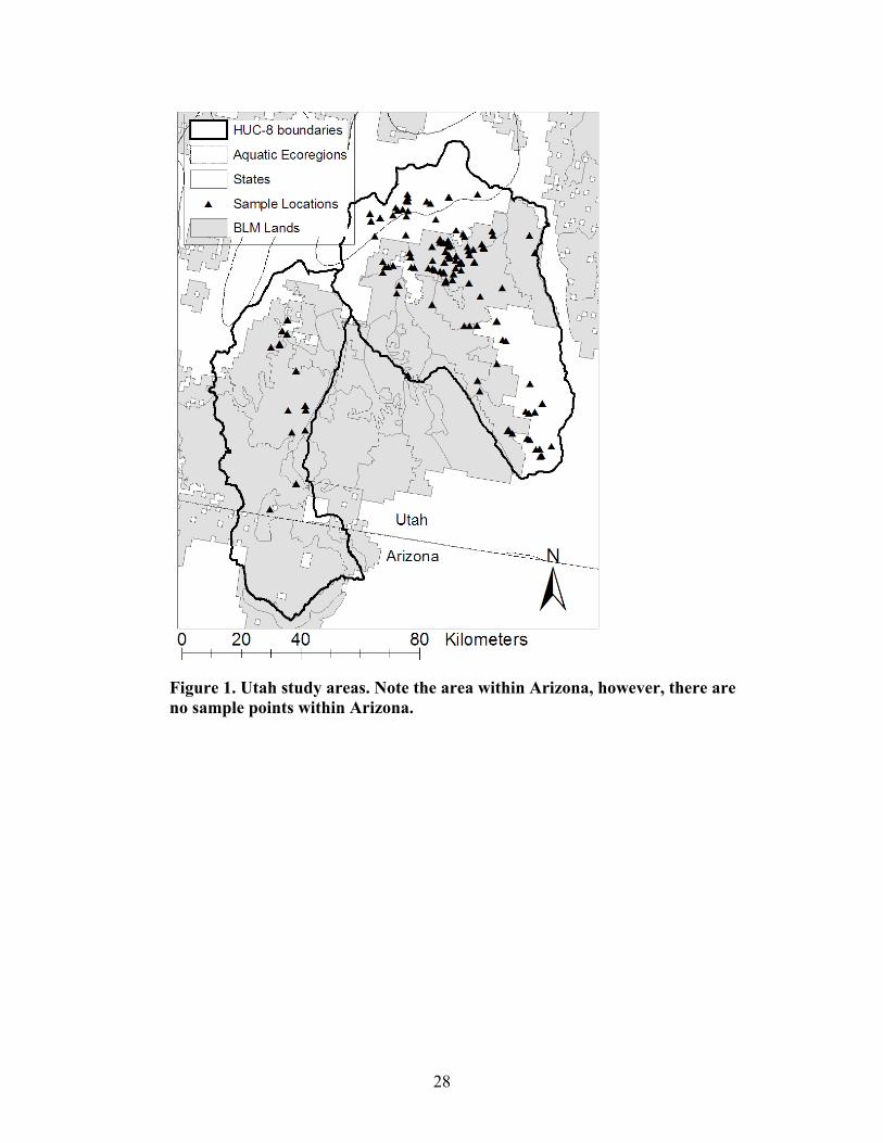
Figure 1. Utah study areas. Note the area within Arizona, however, there are no sample points within Arizona.

28

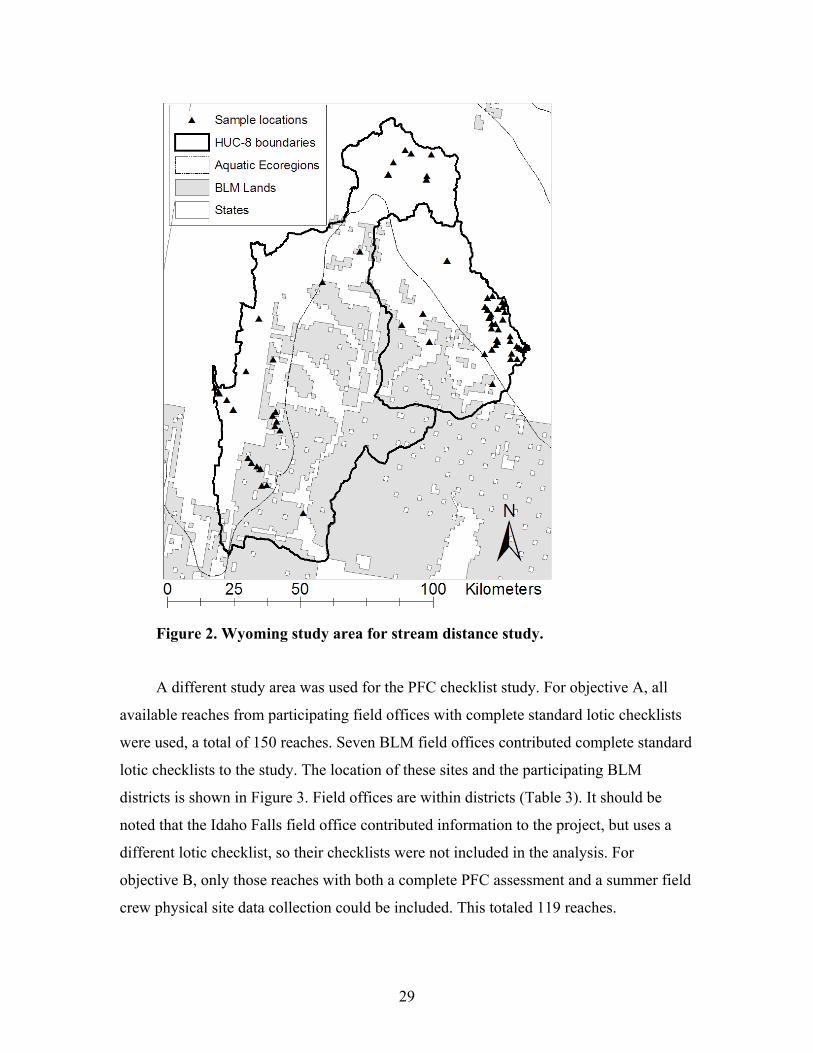
Figure 2. Wyoming study area for stream distance study.

A different study area was used for the PFC checklist study. For objective A, all

available reaches from participating field offices with complete standard lotic checklists

were used, a total of 150 reaches. Seven BLM field offices contributed complete standard

lotic checklists to the study. The location of these sites and the participating BLM

districts is shown in Figure 3. Field offices are within districts (Table 3). It should be

noted that the Idaho Falls field office contributed information to the project, but uses a

different lotic checklist, so their checklists were not included in the analysis. For

objective B, only those reaches with both a complete PFC assessment and a summer field

crew physical site data collection could be included. This totaled 119 reaches.

29

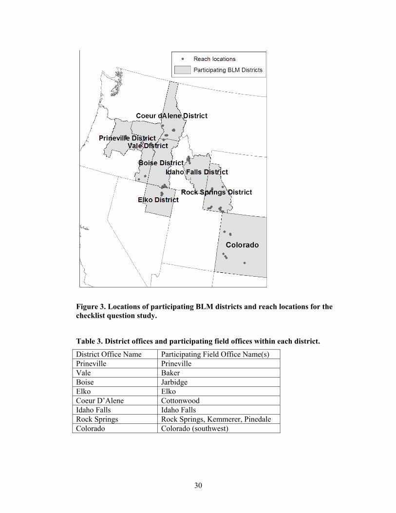
Figure 3. Locations of participating BLM districts and reach locations for the checklist question study.

Table 3. District offices and participating field offices within each district.

District Office Name Participating Field Office Name(s) Prineville Prineville Vale Baker Boise Jarbidge Elko Elko Coeur D’Alene Cottonwood Idaho Falls Idaho Falls Rock Springs Rock Springs, Kemmerer, Pinedale Colorado Colorado (southwest)

30

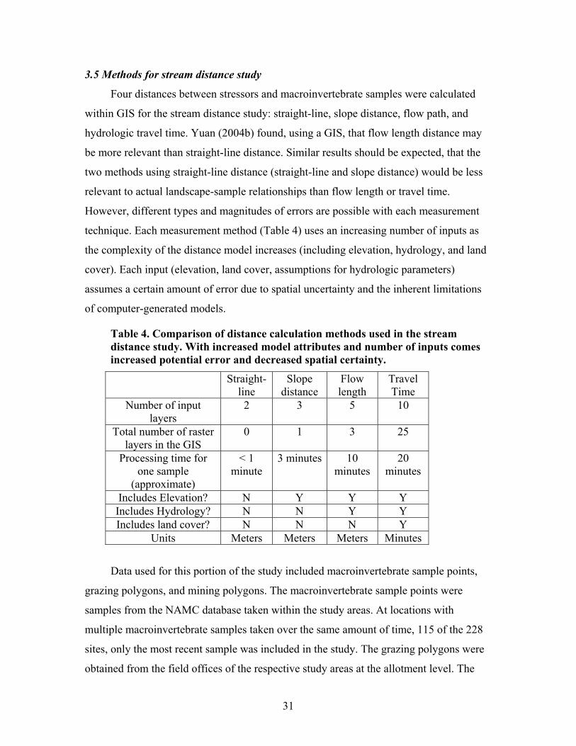
3.5 Methods for stream distance study

Four distances between stressors and macroinvertebrate samples were calculated

within GIS for the stream distance study: straight-line, slope distance, flow path, and

hydrologic travel time. Yuan (2004b) found, using a GIS, that flow length distance may

be more relevant than straight-line distance. Similar results should be expected, that the

two methods using straight-line distance (straight-line and slope distance) would be less

relevant to actual landscape-sample relationships than flow length or travel time.

However, different types and magnitudes of errors are possible with each measurement

technique. Each measurement method (Table 4) uses an increasing number of inputs as

the complexity of the distance model increases (including elevation, hydrology, and land

cover). Each input (elevation, land cover, assumptions for hydrologic parameters)

assumes a certain amount of error due to spatial uncertainty and the inherent limitations

of computer-generated models.

Table 4. Comparison of distance calculation methods used in the stream distance study. With increased model attributes and number of inputs comes increased potential error and decreased spatial certainty.

Straight-line

Slope distance

Flow length

Travel Time

Number of input layers

2 3 5 10

Total number of raster layers in the GIS

0 1 3 25

Processing time for one sample

(approximate)

< 1 minute

3 minutes 10 minutes

20 minutes

Includes Elevation? N Y Y Y Includes Hydrology? N N Y Y Includes land cover? N N N Y

Units Meters Meters Meters Minutes

Data used for this portion of the study included macroinvertebrate sample points,

grazing polygons, and mining polygons. The macroinvertebrate sample points were

samples from the NAMC database taken within the study areas. At locations with

multiple macroinvertebrate samples taken over the same amount of time, 115 of the 228

sites, only the most recent sample was included in the study. The grazing polygons were

obtained from the field offices of the respective study areas at the allotment level. The

31

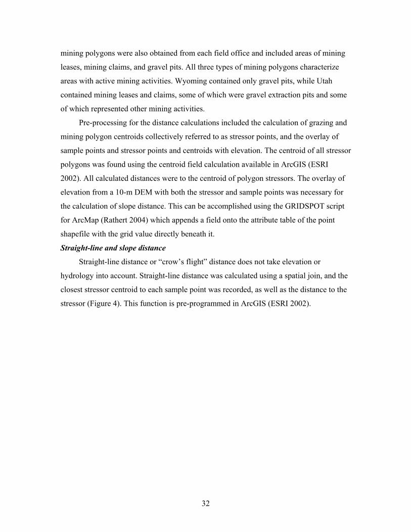
mining polygons were also obtained from each field office and included areas of mining

leases, mining claims, and gravel pits. All three types of mining polygons characterize

areas with active mining activities. Wyoming contained only gravel pits, while Utah

contained mining leases and claims, some of which were gravel extraction pits and some

of which represented other mining activities.

Pre-processing for the distance calculations included the calculation of grazing and

mining polygon centroids collectively referred to as stressor points, and the overlay of

sample points and stressor points and centroids with elevation. The centroid of all stressor

polygons was found using the centroid field calculation available in ArcGIS (ESRI

2002). All calculated distances were to the centroid of polygon stressors. The overlay of

elevation from a 10-m DEM with both the stressor and sample points was necessary for

the calculation of slope distance. This can be accomplished using the GRIDSPOT script

for ArcMap (Rathert 2004) which appends a field onto the attribute table of the point

shapefile with the grid value directly beneath it.

Straight-line and slope distance

Straight-line distance or “crow’s flight” distance does not take elevation or

hydrology into account. Straight-line distance was calculated using a spatial join, and the

closest stressor centroid to each sample point was recorded, as well as the distance to the

stressor (Figure 4). This function is pre-programmed in ArcGIS (ESRI 2002).

32

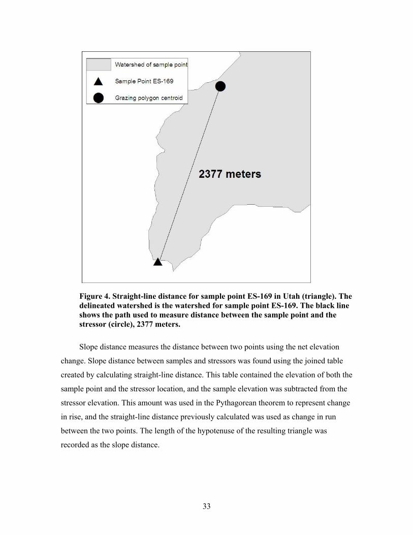
Figure 4. Straight-line distance for sample point ES-169 in Utah (triangle). The delineated watershed is the watershed for sample point ES-169. The black line shows the path used to measure distance between the sample point and the stressor (circle), 2377 meters.

Slope distance measures the distance between two points using the net elevation

change. Slope distance between samples and stressors was found using the joined table

created by calculating straight-line distance. This table contained the elevation of both the

sample point and the stressor location, and the sample elevation was subtracted from the

stressor elevation. This amount was used in the Pythagorean theorem to represent change

in rise, and the straight-line distance previously calculated was used as change in run

between the two points. The length of the hypotenuse of the resulting triangle was

recorded as the slope distance.

33

Flow length

Flow length takes elevation and topography information into account. This is

accomplished within a GIS by first calculating the flow direction of each cell within the

watersheds of interest using a DEM. Flow direction is calculated for one nine-cell block,

or neighborhood, at a time. A pre-programmed algorithm computes all calculations for

flow length. The flow direction is defined as the steepest downhill slope from the center

cell (ESRI 2002). From the flow direction, the length of the path water would take to an

outlet can be determined. In this case, outlets were the macroinvertebrate sample points.

Flow length distance was calculated using the flow length command available in Raster

Calculator in ArcMap (ESRI 2002) (Figure 5). The downstream distance was calculated

from each stressor to the closest outlet point, or sample. GRIDSPOT was used to record

the distance to outlet at each stressor location.

34

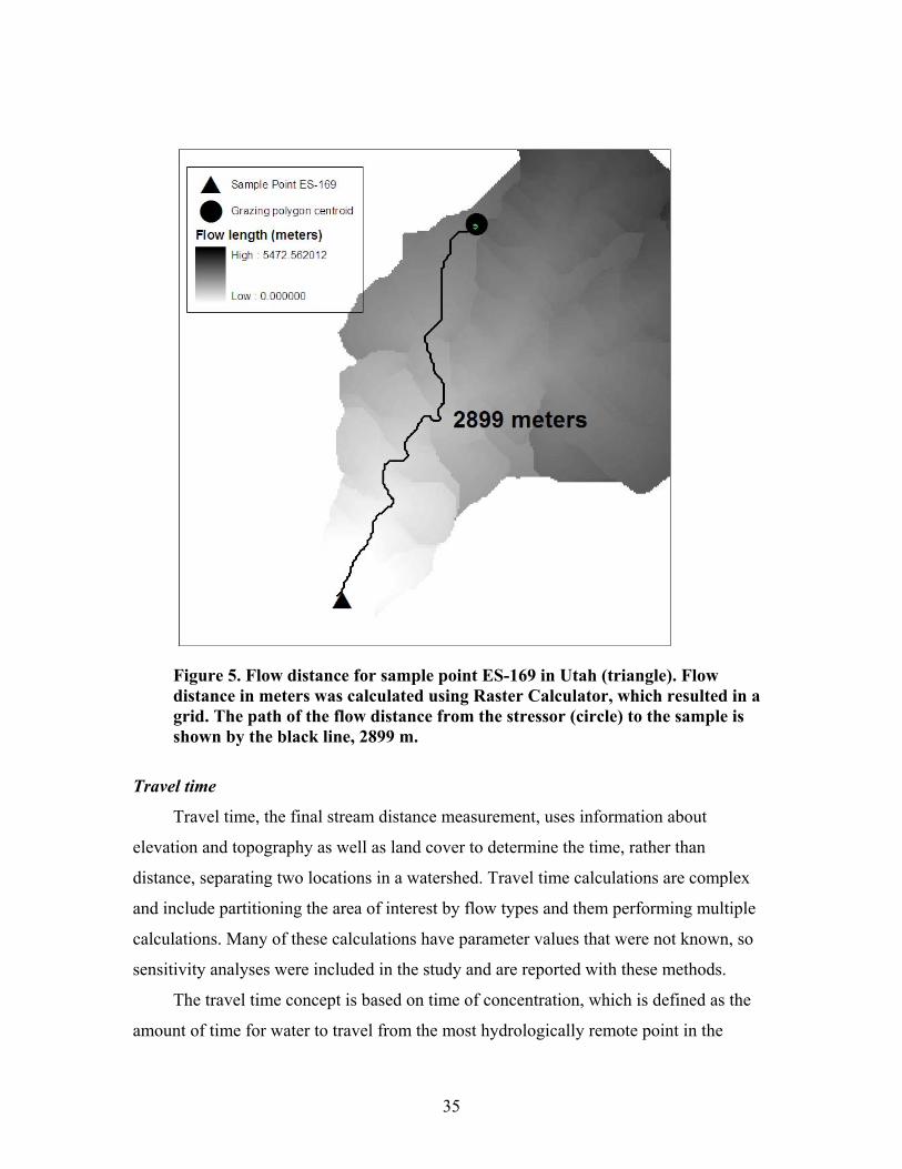
Figure 5. Flow distance for sample point ES-169 in Utah (triangle). Flow distance in meters was calculated using Raster Calculator, which resulted in a grid. The path of the flow distance from the stressor (circle) to the sample is shown by the black line, 2899 m.

Travel time

Travel time, the final stream distance measurement, uses information about

elevation and topography as well as land cover to determine the time, rather than

distance, separating two locations in a watershed. Travel time calculations are complex

and include partitioning the area of interest by flow types and them performing multiple

calculations. Many of these calculations have parameter values that were not known, so

sensitivity analyses were included in the study and are reported with these methods.

The travel time concept is based on time of concentration, which is defined as the

amount of time for water to travel from the most hydrologically remote point in the

35

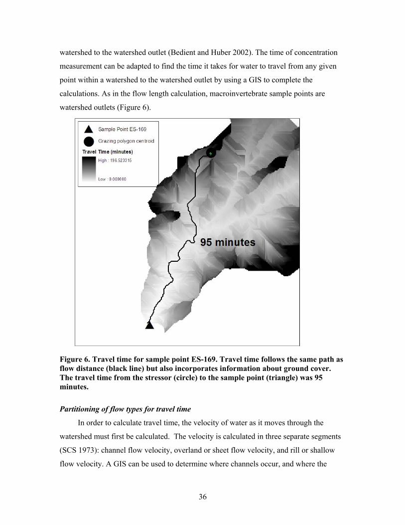
watershed to the watershed outlet (Bedient and Huber 2002). The time of concentration

measurement can be adapted to find the time it takes for water to travel from any given

point within a watershed to the watershed outlet by using a GIS to complete the

calculations. As in the flow length calculation, macroinvertebrate sample points are

watershed outlets (Figure 6).

Figure 6. Travel time for sample point ES-169. Travel time follows the same path as flow distance (black line) but also incorporates information about ground cover. The travel time from the stressor (circle) to the sample point (triangle) was 95 minutes. Partitioning of flow types for travel time

In order to calculate travel time, the velocity of water as it moves through the

watershed must first be calculated. The velocity is calculated in three separate segments

(SCS 1973): channel flow velocity, overland or sheet flow velocity, and rill or shallow

flow velocity. A GIS can be used to determine where channels occur, and where the

36

separation between overland and shallow flow occurs. Each 10 by 10-meter cell in a

watershed represents only one type of flow. The resulting grid from the GIS operations to

separate the three types of flow will be referred to as a partition grid. The partition grid

will contain an integer in each cell designating which of the three types of flow occurred

in that grid cell. Channel locations can be determined using a flow accumulation grid

produced using a pre-programmed function in GIS (ESRI 2002). Flow accumulation is

calculated using flow direction (see above) and based on the direction of flow and the

position of the cell in the watershed, measures the number of cells “flowing” into that

cell. This is calculated for every cell in the watershed, resulting in a flow accumulation

grid. This can be used to estimate channel location, were cells with high flow

accumulations are assumed to be channels. To separate channels from non-channels, a

conditional statement it used based on the minimum flow accumulation a cell must have

to be considered a channel. This minimum flow accumulation will be referred to as the

flow accumulation cutoff, or FA cutoff. The resulting flow network will be referred to as

a digital elevation model-generated flow network, or a DEM-FN. A sensitivity analysis

was performed on each HUC8 in the study area to determine the most desirable FA

cutoff. One subwatershed in each HUC8 was chosen. The subwatersheds were each about

25,000 ha in area, and were chosen to represent the upper to middle reaches of the entire

study areas.

A USGS Digital Raster Graphic (DRG) was used as a reference to determine the

most desirable FA cutoff for the DEM-FN. The most desirable FA cutoff would be that

which most closely aligns with the DRG stream channel. A DRG is a scanned and

rasterized USGS topographic quad that shows all intermittent stream channels marked by

the USGS and was assumed to represent ground truth for the purposes of this study. For

each subwatershed, the stream color was separated out of the DRG and ArcScan was

used to generate a continuous network. Then, DEM-FN were generated at the FA

thresholds of 200, 400, 800, 1000,1400, 1600, and 2000 (10 m cells). Each DEM-FN was

overlaid on the DRG-FN to visually determine which DEM-FN had the best match to the

intermittent stream networks from the DRG.

For Utah subwatershed 1, the FA cutoff of 800 cells appeared to give the closest

match (Figure 7). In Utah subwatershed 2, the FA cutoff of 1600 cells appeared to best

37

match the DRG-FN, however, results are not as clearly interpretable as for subwatershed

1. In Wyoming subwatershed 1, an FA cutoff of 2000 cells was chosen as the best

representation of the DRG flow network, and in Wyoming subwatershed 2, an FA cutoff

of 1600 cells was chosen. In Utah 1 and Wyoming 1, choosing the DEM-FN was

relatively straightforward. The flow network lengths were relatively homogeneous

throughout the watershed and closely matched the DRG-FN in almost all areas.

However, in Utah 2 and Wyoming 2 there were many areas that were erroneous, due to

lack of relief in the DEM and due to water bodies other than streams in the DRG. These

errors also made a qualitative approach to choosing a FA cutoff difficult. When faced

with such a watershed, and an appropriate FA cutoff is not obvious, the analyst should

choose a reasonable FA cutoff (between 200 and 2000 cells) that appears to best

represent the stream network as a whole. It is the author’s opinion that each HUC8 should

be tested for the most appropriate FA cutoff, as the FA cutoff will change according to

climatic and topographical differences, even among adjacent HUC8s.

38

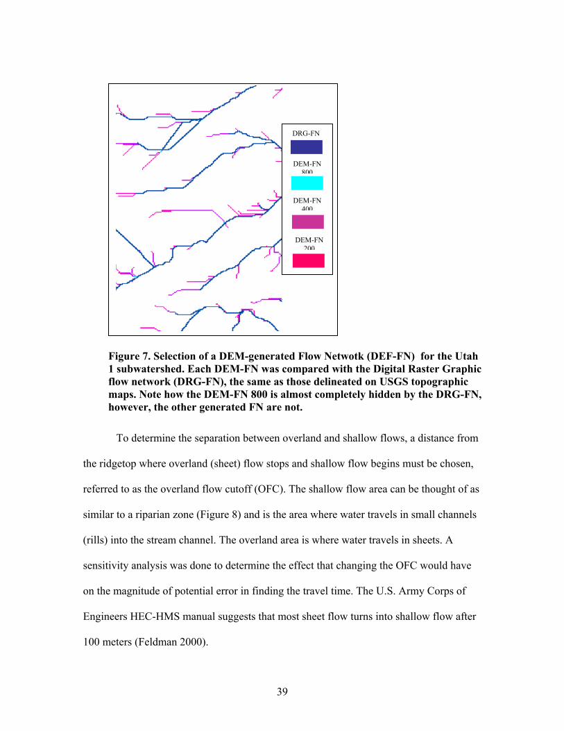
DRG-FN

DEM-FN 800

DEM-FN 400

DEM-FN 200

Figure 7. Selection of a DEM-generated Flow Netwotk (DEF-FN) for the Utah 1 subwatershed. Each DEM-FN was compared with the Digital Raster Graphic flow network (DRG-FN), the same as those delineated on USGS topographic maps. Note how the DEM-FN 800 is almost completely hidden by the DRG-FN, however, the other generated FN are not.

To determine the separation between overland and shallow flows, a distance from

the ridgetop where overland (sheet) flow stops and shallow flow begins must be chosen,

referred to as the overland flow cutoff (OFC). The shallow flow area can be thought of as

similar to a riparian zone (Figure 8) and is the area where water travels in small channels

(rills) into the stream channel. The overland area is where water travels in sheets. A

sensitivity analysis was done to determine the effect that changing the OFC would have

on the magnitude of potential error in finding the travel time. The U.S. Army Corps of

Engineers HEC-HMS manual suggests that most sheet flow turns into shallow flow after

100 meters (Feldman 2000).

39

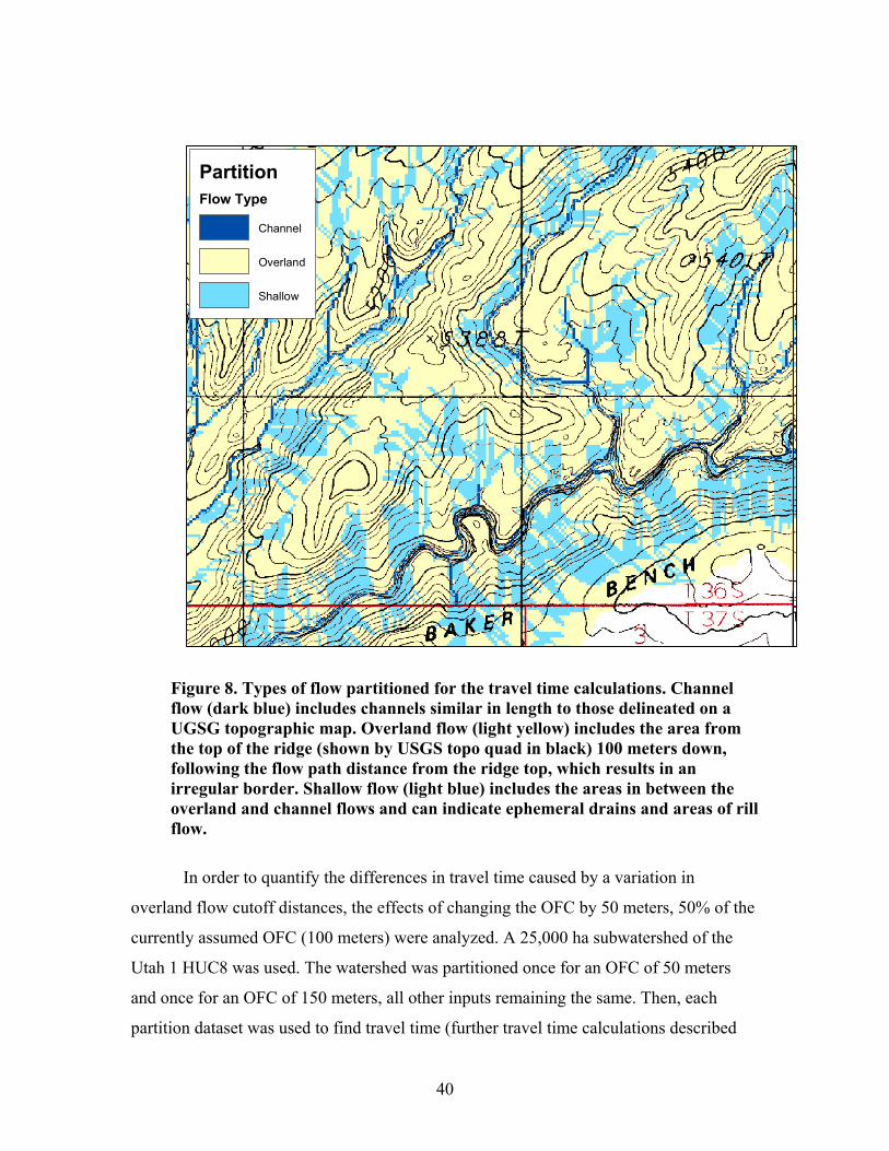
PartitionFlow Type

Channel

Overland

Shallow

Figure 8. Types of flow partitioned for the travel time calculations. Channel flow (dark blue) includes channels similar in length to those delineated on a UGSG topographic map. Overland flow (light yellow) includes the area from the top of the ridge (shown by USGS topo quad in black) 100 meters down, following the flow path distance from the ridge top, which results in an irregular border. Shallow flow (light blue) includes the areas in between the overland and channel flows and can indicate ephemeral drains and areas of rill flow.

In order to quantify the differences in travel time caused by a variation in

overland flow cutoff distances, the effects of changing the OFC by 50 meters, 50% of the

currently assumed OFC (100 meters) were analyzed. A 25,000 ha subwatershed of the

Utah 1 HUC8 was used. The watershed was partitioned once for an OFC of 50 meters

and once for an OFC of 150 meters, all other inputs remaining the same. Then, each

partition dataset was used to find travel time (further travel time calculations described

40

hereafter). The travel time results were compiled and the mean travel time for the

watershed was found. The mean travel time for the 50-meter OFC was 132 minutes and

the mean travel time for the 150-meter OFC was 133 minutes. Since less than one minute

(0.7 %) mean difference between 50 meter and 150 meter OFC’s were found in the final

travel time, this study assumes that an overland flow distance of 100 meters will be

sufficient and appropriate as suggested in the HEC-HMS manual (Feldman 2000). If

ground truth data or researcher knowledge in this area improves, then other distances

should be tested for their final effect on travel times.

Computing channel velocity for travel time

Once the partitioning of flow types was complete, velocity was computed for each

separate flow type: channel, shallow, and overland. To determine channel velocity,

Manning’s equation was used:

Vchannel= (CR2/3S1/2)/n;

where R= Hydraulic radius of the stream,

S= slope of stream channel, and

n= Manning roughness coefficient (Feldman 2000, Haan et al. 1994).

Hydraulic radius was determined by the equation

R = A/Wp,

where A is the cross-sectional area of the stream channel and Wp is the wetted perimeter

of the cross-sectional area. This calculation presents some problems when incorporated

into a GIS. First, R changes slightly at each cross-section along a stream network, so the

possible values of R within a study area are nearly infinite. Additionally, velocity and

channel dimensions are dependent on R (as calculated here) but R is also dependent on

velocity. Therefore, some generalizations must be made about the average R based on

assumptions about flow in a study area. Additionally, the resolution of the DEMs used in

this study is too coarse to be used in determining stream widths and depths. However,

equations are available for most regions that relate channel properties, such as width and

depth, and sometimes R directly to watershed properties, such as drainage area. Drainage

area can be calculated in a GIS and then a regional flow equation can be used to

determine average channel width and depth, or R if available, from the drainage area. If

an equation for R is not available, then the width and depth can be used to find the area

41

and wetted perimeter of the stream after a representative stream cross-sectional shape is

chosen from those listed in Rosgen (1994) and a simplified R value can be calculated.

The regional flow equation used for Wyoming was from Lowham (1976). Lowham

used regions to separate areas of Wyoming that were largely different in hydrologic

regime. The region used for this study was region 1, or the Wyoming mountainous areas.

Lowham calculated hydraulic radius (R) at each gauging station used for data collection

in region 1. Lowham assumed from his observations Rosgen stream type B, a moderately

entrenched triangular shape with a high width: depth ratio, and both streambanks

generally at equal angles to the stream bottom. The equation

log10R = 0.1170357 + 0.4583036 log10DA;

where DA = acres of drainage area, was used and had an r2 value of 0.78 (Lowham

1976). Individual equations for width and depth were also available, but had lower r2

values than the equation for R and would introduce more potential error into the final

calculation.

The regional flow equations used for Utah were from Fields (1975). The

equations

W = 3.27 * DA 0.51 (r2 = 0.83) and

D = 0.79 * DA0.24 (r2 = 0.58)

where W = stream width in feet and

D = stream depth in feet were used (Fields 1975).

A Rosgen (1994) stream type of B was used and the equation used to determine R was:

R = (1/2W2 + D2)/2

substituting the W and D equations above. An equation for R directly from drainage area

would have been ideal, however, no such information was found in the literature.

A sensitivity analysis was performed to determine the effect that the choice of

stream shape for calculating an approximate hydraulic radius would have on travel time.

Ideally, flow rate could be held constant with R calculated for differing channel shapes.

However, flow rate (velocity) is the ultimate product in this calculation, so channel cross-

sectional area will be used as a constant. The change in R given a constant cross-sectional

channel area (4 m2) across five common channel shapes, corresponding to Rosgen stream

types, was calculated (Table 5). Travel time was calculated twice, once using the

42

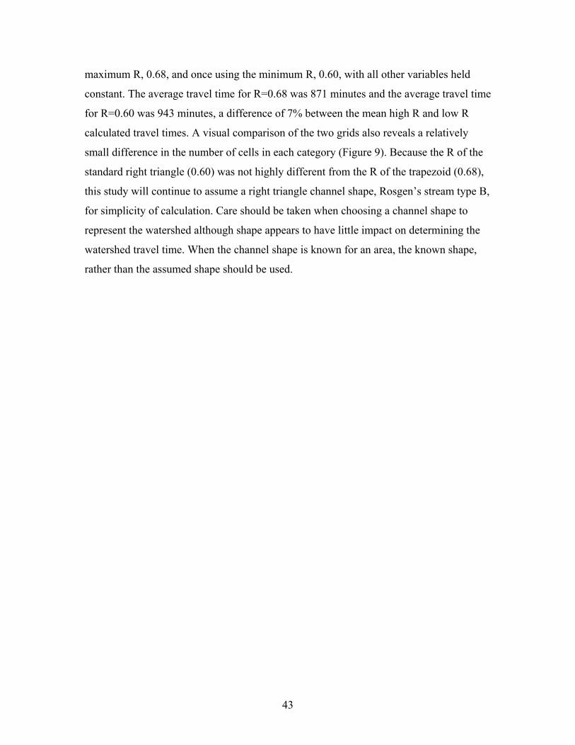
maximum R, 0.68, and once using the minimum R, 0.60, with all other variables held

constant. The average travel time for R=0.68 was 871 minutes and the average travel time

for R=0.60 was 943 minutes, a difference of 7% between the mean high R and low R

calculated travel times. A visual comparison of the two grids also reveals a relatively

small difference in the number of cells in each category (Figure 9). Because the R of the

standard right triangle (0.60) was not highly different from the R of the trapezoid (0.68),

this study will continue to assume a right triangle channel shape, Rosgen’s stream type B,

for simplicity of calculation. Care should be taken when choosing a channel shape to

represent the watershed although shape appears to have little impact on determining the

watershed travel time. When the channel shape is known for an area, the known shape,

rather than the assumed shape should be used.

43

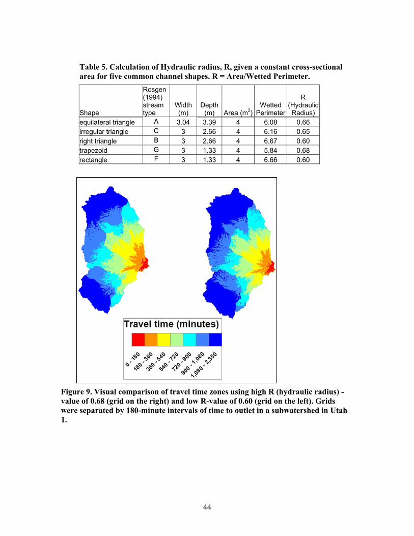
Table 5. Calculation of Hydraulic radius, R, given a constant cross-sectional area for five common channel shapes. R = Area/Wetted Perimeter.

Shape

Rosgen (1994) stream type

Width (m)

Depth (m) Area (m2)

Wetted Perimeter

R (Hydraulic Radius)

equilateral triangle A 3.04 3.39 4 6.08 0.66 irregular triangle C 3 2.66 4 6.16 0.65 right triangle B 3 2.66 4 6.67 0.60 trapezoid G 3 1.33 4 5.84 0.68 rectangle F 3 1.33 4 6.66 0.60

Figure 9. Visual comparison of travel time zones using high R (hydraulic radius) -value of 0.68 (grid on the right) and low R-value of 0.60 (grid on the left). Grids were separated by 180-minute intervals of time to outlet in a subwatershed in Utah 1.

44

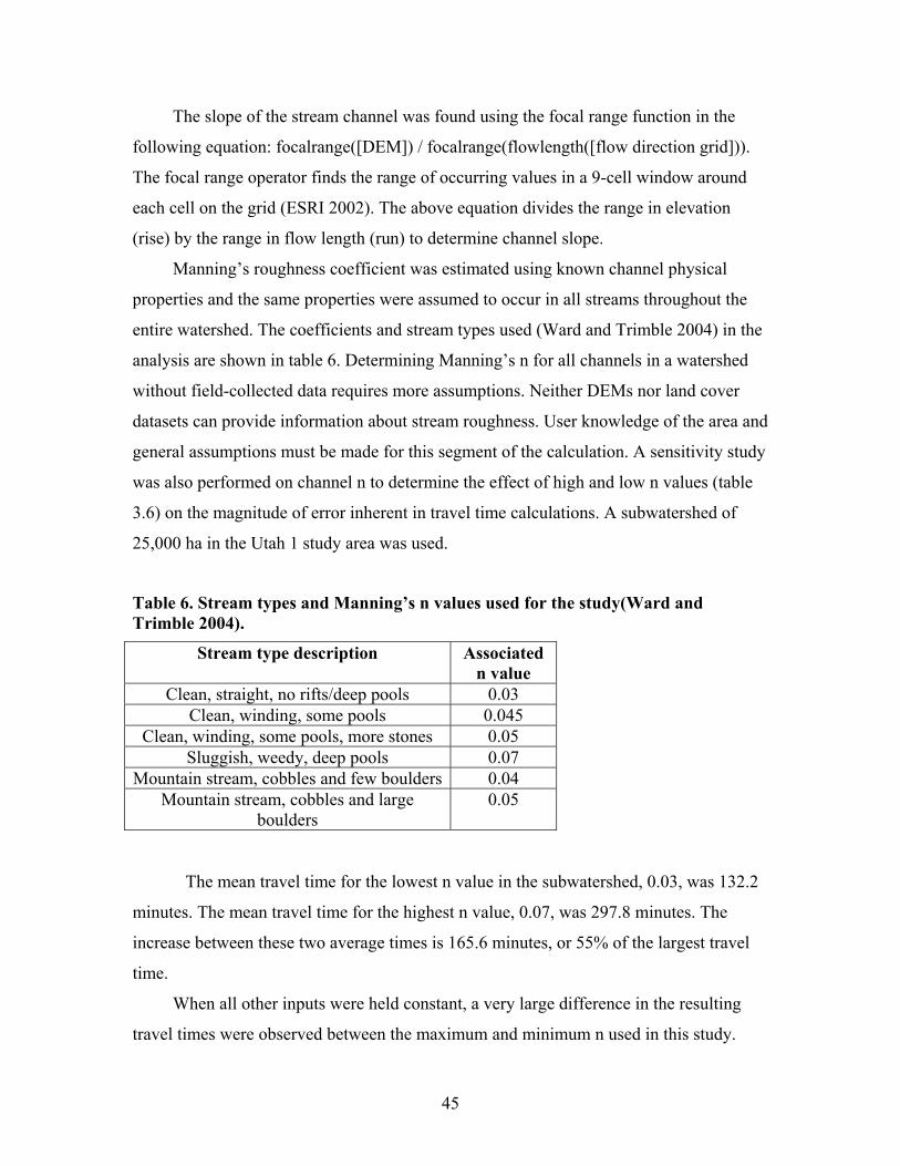
The slope of the stream channel was found using the focal range function in the

following equation: focalrange([DEM]) / focalrange(flowlength([flow direction grid])).

The focal range operator finds the range of occurring values in a 9-cell window around

each cell on the grid (ESRI 2002). The above equation divides the range in elevation

(rise) by the range in flow length (run) to determine channel slope.

Manning’s roughness coefficient was estimated using known channel physical

properties and the same properties were assumed to occur in all streams throughout the

entire watershed. The coefficients and stream types used (Ward and Trimble 2004) in the

analysis are shown in table 6. Determining Manning’s n for all channels in a watershed

without field-collected data requires more assumptions. Neither DEMs nor land cover

datasets can provide information about stream roughness. User knowledge of the area and

general assumptions must be made for this segment of the calculation. A sensitivity study

was also performed on channel n to determine the effect of high and low n values (table

3.6) on the magnitude of error inherent in travel time calculations. A subwatershed of

25,000 ha in the Utah 1 study area was used.

Table 6. Stream types and Manning’s n values used for the study(Ward and Trimble 2004).

Stream type description Associated n value

Clean, straight, no rifts/deep pools 0.03 Clean, winding, some pools 0.045

Clean, winding, some pools, more stones 0.05 Sluggish, weedy, deep pools 0.07

Mountain stream, cobbles and few boulders 0.04 Mountain stream, cobbles and large

boulders 0.05

The mean travel time for the lowest n value in the subwatershed, 0.03, was 132.2

minutes. The mean travel time for the highest n value, 0.07, was 297.8 minutes. The

increase between these two average times is 165.6 minutes, or 55% of the largest travel

time.

When all other inputs were held constant, a very large difference in the resulting

travel times were observed between the maximum and minimum n used in this study.

45

This illustrates that the travel time calculation is very sensitive to the input of channel n,

determined by the channel type. For this study, because dominant channel type is not

known, an n value of 0.05 “Clean, winding, some pools, more stones” and “Mountain

stream, cobbles and large boulders”(Ward and Trimble 2004) will be assumed. This n

value was chosen because it avoids the extremes of the n values available and it is viable

for two distinctly different stream types. Researcher knowledge of the stream type would

have been preferable, but was beyond the sampling scope of this study.

Computing shallow and overland velocities for travel time

The velocity of cells in the watershed partitioned as shallow flow was calculated as:

Vshallow =16.1345(sqrt S) for unpaved areas and =20.3282(sqrt S) for paved areas, where:

S= percent land slope (Feldman 2000). Paved and unpaved areas were determined using

GAP data (Table 2). Areas classified as urban, suburban industrial, or commercial were

considered “paved” areas and all other classifications “unpaved”. Percent land slope was

determined using the pre-programmed slope function in ArcGIS, which uses the Z-values

(elevation) of an eight-cell neighborhood surrounding each cell to determine the slope of

that cell. Cells directly adjacent to the center cell are weighted more heavily than the cells

diagonal to the center cell (ESRI 2002).

The velocity of cells partitioned as overland (sheet) flow was determined by:

Voverland= (Lm/((0.007 (nL)0.8)/(P20.5*S0.4)))/60 where: Lm = flow length to outlet in

meters; n= Manning’s roughness coefficient for land; L= flow length to outlet in feet;

P2=2-year, 24-hour rainfall; S= percent land slope (Feldman 2000, Haan et al. 1994,

Heatwole and Burcher 2003).

Manning’s roughness coefficient for the land surface was found using GAP data to

determine land cover, and Manning’s n charts for each land cover type provided in a

hydrology text (Ward and Trimble 2004). Land cover types in the Manning’s n chart did

not exactly match the GAP categories for either state, so some assumptions were made to

assign n values to each land cover type present in the study areas (Table 7 and Table 8).

There were also differences in the detail of coverage between the two states, where

Wyoming had many detailed cover types and Utah had fewer, less detailed cover types.

46

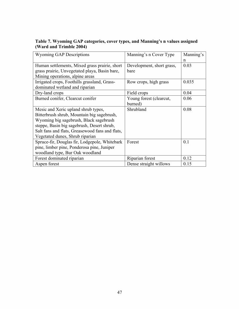
Table 7. Wyoming GAP categories, cover types, and Manning’s n values assigned (Ward and Trimble 2004)

Wyoming GAP Descriptions Manning’s n Cover Type Manning’s n

Human settlements, Mixed grass prairie, short grass prairie, Unvegetated playa, Basin bare, Mining operations, alpine areas

Development, short grass, bare

0.03

Irrigated crops, Foothills grassland, Grass-dominated wetland and riparian

Row crops, high grass 0.035

Dry-land crops Field crops 0.04 Burned conifer, Clearcut conifer Young forest (clearcut,

burned) 0.06

Mesic and Xeric upland shrub types, Bitterbrush shrub, Mountain big sagebrush, Wyoming big sagebrush, Black sagebrush steppe, Basin big sagebrush, Desert shrub, Salt fans and flats, Greasewood fans and flats, Vegetated dunes, Shrub riparian

Shrubland 0.08

Spruce-fir, Douglas fir, Lodgepole, Whitebark pine, limber pine, Ponderosa pine, Juniper woodland type, Bur Oak woodland

Forest 0.1

Forest dominated riparian Riparian forest 0.12 Aspen forest Dense straight willows 0.15

47

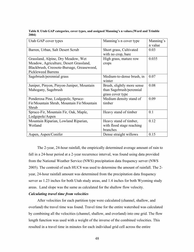
Table 8. Utah GAP categories, cover types, and assigned Manning’s n values.(Ward and Trimble 2004)

Utah GAP cover types Manning’s n cover type Manning’s n value

Barren, Urban, Salt Desert Scrub Short grass, Cultivated with no crop, bare

0.03

Grassland, Alpine, Dry Meadow, Wet Meadow, Agriculture, Desert Grassland, Blackbrush, Creosote-Bursage, Greasewood, Pickleweed Barrens

High grass, mature row crops

0.035

Sagebrush/perennial grass Medium-to-dense brush, in winter

0.07

Juniper, Pinyon, Pinyon-Juniper, Mountain Mahogany, Sagebrush

Brush, slightly more sense than Sagebrush/perennial grass cover type

0.08

Ponderosa Pine, Lodgepole, Spruce-Fir/Mountain Shrub, Mountain Fir/Mountain Shrub

Medium density stand of timber

0.09

Spruce-Fir, Mountain Fir, Oak, Maple, Lodgepole/Aspen

Heavy stand of timber 0.1

Mountain Riparian, Lowland Riparian, Wetland

Heavy stand of timber, with flood stage reaching branches

0.12

Aspen, Aspen/Conifer Dense straight willows 0.15

The 2-year, 24-hour rainfall, the empirically determined average amount of rain to

fall in a 24-hour period at a 2-year recurrence interval, was found using data provided

from the National Weather Service (NWS) precipitation data frequency server (NWS

2005). The centroid of each HUC8 was used to determine the amount of rainfall. The 2-

year, 24-hour rainfall amount was determined from the precipitation data frequency

server as 1.23 inches for both Utah study areas, and 1.4 inches for both Wyoming study

areas. Land slope was the same as calculated for the shallow flow velocity.

Calculating travel time from velocities

After velocities for each partition type were calculated (channel, shallow, and

overland) the travel time was found. Travel time for the entire watershed was calculated

by combining all the velocities (channel, shallow, and overland) into one grid. The flow

length function was used with a weight of the inverse of the combined velocities. This

resulted in a travel time in minutes for each individual grid cell across the entire

48

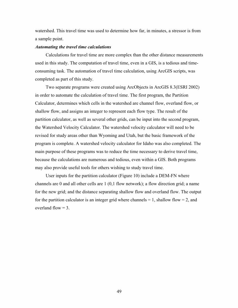
watershed. This travel time was used to determine how far, in minutes, a stressor is from

a sample point.

Automating the travel time calculations

Calculations for travel time are more complex than the other distance measurements

used in this study. The computation of travel time, even in a GIS, is a tedious and time-

consuming task. The automation of travel time calculation, using ArcGIS scripts, was

completed as part of this study.

Two separate programs were created using ArcObjects in ArcGIS 8.3(ESRI 2002)

in order to automate the calculation of travel time. The first program, the Partition

Calculator, determines which cells in the watershed are channel flow, overland flow, or

shallow flow, and assigns an integer to represent each flow type. The result of the

partition calculator, as well as several other grids, can be input into the second program,

the Watershed Velocity Calculator. The watershed velocity calculator will need to be

revised for study areas other than Wyoming and Utah, but the basic framework of the

program is complete. A watershed velocity calculator for Idaho was also completed. The

main purpose of these programs was to reduce the time necessary to derive travel time,

because the calculations are numerous and tedious, even within a GIS. Both programs

may also provide useful tools for others wishing to study travel time.

User inputs for the partition calculator (Figure 10) include a DEM-FN where

channels are 0 and all other cells are 1 (0,1 flow network); a flow direction grid; a name

for the new grid; and the distance separating shallow flow and overland flow. The output

for the partition calculator is an integer grid where channels = 1, shallow flow = 2, and

overland flow = 3.

49

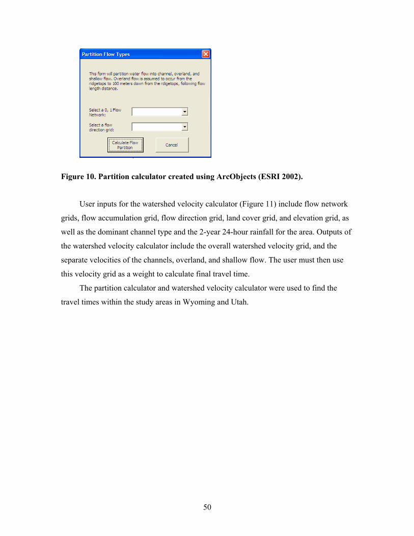
Figure 10. Partition calculator created using ArcObjects (ESRI 2002).

User inputs for the watershed velocity calculator (Figure 11) include flow network

grids, flow accumulation grid, flow direction grid, land cover grid, and elevation grid, as

well as the dominant channel type and the 2-year 24-hour rainfall for the area. Outputs of

the watershed velocity calculator include the overall watershed velocity grid, and the

separate velocities of the channels, overland, and shallow flow. The user must then use

this velocity grid as a weight to calculate final travel time.

The partition calculator and watershed velocity calculator were used to find the

travel times within the study areas in Wyoming and Utah.

50

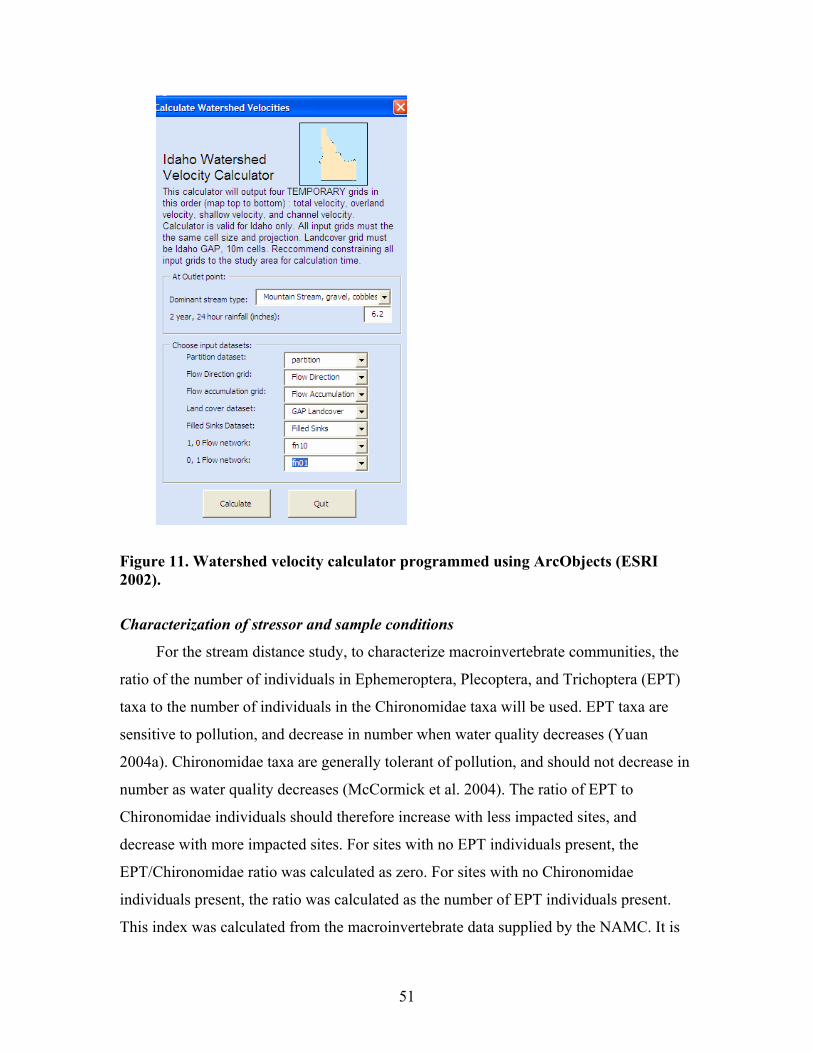
Figure 11. Watershed velocity calculator programmed using ArcObjects (ESRI 2002). Characterization of stressor and sample conditions

For the stream distance study, to characterize macroinvertebrate communities, the

ratio of the number of individuals in Ephemeroptera, Plecoptera, and Trichoptera (EPT)

taxa to the number of individuals in the Chironomidae taxa will be used. EPT taxa are

sensitive to pollution, and decrease in number when water quality decreases (Yuan

2004a). Chironomidae taxa are generally tolerant of pollution, and should not decrease in

number as water quality decreases (McCormick et al. 2004). The ratio of EPT to

Chironomidae individuals should therefore increase with less impacted sites, and

decrease with more impacted sites. For sites with no EPT individuals present, the

EPT/Chironomidae ratio was calculated as zero. For sites with no Chironomidae

individuals present, the ratio was calculated as the number of EPT individuals present.

This index was calculated from the macroinvertebrate data supplied by the NAMC. It is

51

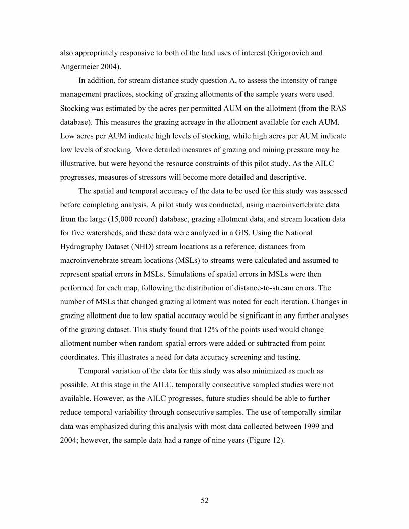
also appropriately responsive to both of the land uses of interest (Grigorovich and

Angermeier 2004).

In addition, for stream distance study question A, to assess the intensity of range

management practices, stocking of grazing allotments of the sample years were used.

Stocking was estimated by the acres per permitted AUM on the allotment (from the RAS

database). This measures the grazing acreage in the allotment available for each AUM.

Low acres per AUM indicate high levels of stocking, while high acres per AUM indicate

low levels of stocking. More detailed measures of grazing and mining pressure may be

illustrative, but were beyond the resource constraints of this pilot study. As the AILC

progresses, measures of stressors will become more detailed and descriptive.

The spatial and temporal accuracy of the data to be used for this study was assessed

before completing analysis. A pilot study was conducted, using macroinvertebrate data

from the large (15,000 record) database, grazing allotment data, and stream location data

for five watersheds, and these data were analyzed in a GIS. Using the National

Hydrography Dataset (NHD) stream locations as a reference, distances from

macroinvertebrate stream locations (MSLs) to streams were calculated and assumed to

represent spatial errors in MSLs. Simulations of spatial errors in MSLs were then

performed for each map, following the distribution of distance-to-stream errors. The

number of MSLs that changed grazing allotment was noted for each iteration. Changes in

grazing allotment due to low spatial accuracy would be significant in any further analyses

of the grazing dataset. This study found that 12% of the points used would change

allotment number when random spatial errors were added or subtracted from point

coordinates. This illustrates a need for data accuracy screening and testing.

Temporal variation of the data for this study was also minimized as much as

possible. At this stage in the AILC, temporally consecutive sampled studies were not

available. However, as the AILC progresses, future studies should be able to further

reduce temporal variability through consecutive samples. The use of temporally similar

data was emphasized during this analysis with most data collected between 1999 and

2004; however, the sample data had a range of nine years (Figure 12).

52

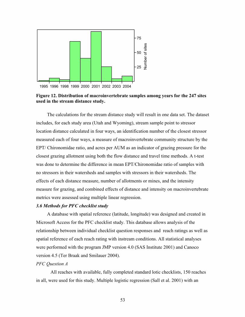
25

50

75

Num

ber o

f site

s

1995 1996 1998 1999 2000 2001 2002 2003 2004 Figure 12. Distribution of macroinvertebrate samples among years for the 247 sites used in the stream distance study.

The calculations for the stream distance study will result in one data set. The dataset

includes, for each study area (Utah and Wyoming), stream sample point to stressor

location distance calculated in four ways, an identification number of the closest stressor

measured each of four ways, a measure of macroinvertebrate community structure by the

EPT/ Chironomidae ratio, and acres per AUM as an indicator of grazing pressure for the

closest grazing allotment using both the flow distance and travel time methods. A t-test

was done to determine the difference in mean EPT/Chironomidae ratio of samples with

no stressors in their watersheds and samples with stressors in their watersheds. The

effects of each distance measure, number of allotments or mines, and the intensity

measure for grazing, and combined effects of distance and intensity on macroinvertebrate

metrics were assessed using multiple linear regression.

3.6 Methods for PFC checklist study

A database with spatial reference (latitude, longitude) was designed and created in

Microsoft Access for the PFC checklist study. This database allows analysis of the

relationship between individual checklist question responses and reach ratings as well as

spatial reference of each reach rating with instream conditions. All statistical analyses

were performed with the program JMP version 4.0 (SAS Institute 2001) and Canoco

version 4.5 (Ter Braak and Smilauer 2004).

PFC Question A

All reaches with available, fully completed standard lotic checklists, 150 reaches

in all, were used for this study. Multiple logistic regression (Sall et al. 2001) with an

53

alpha level of 0.05 was used to find the relationship between the reach rating (dependent

variable) and each checklist question (independent variables). Ordinal logistic regression

was used in place of binary logistic regression (often referred to as simply logistic

regression) because the response variable has more than two categories and the

explanatory variables have any number of categories. In this case, the response variable is

PFC rating with three possible categories, and the explanatory variables are the 17

checklist questions, each with three possible categories as well. Apparent trends for the

FAR category (downward, upward, not apparent) were ignored in this analysis because of

the inconsistency between observers in assigning apparent trends. The log odds between

the three separate categories are simulated at the same time in multiple ordinal logistic

regression. For example, log odds of PFC vs. FAR, FAR vs. NF, and NF vs. PFC are all

estimated together.

Principal components analysis was also used to illustrate any response patterns.

PCA analysis produces a biplot with multiple axes, where axes represent eigenvalues,

which are composites of several variables, arrows represent checklist questions, and

points on the plot represent sample points. In a PCA biplot, the length of the arrows

indicates the strength of the question’s relationship to the PCA axes. The direction of the

question’s arrow in relationship to the other arrows indicates the degree of association

with other questions; where arrows with a large angle of separation are less likely to be

associated, and those with a small angle of separation are more likely to be associated.

Axes were scaled in the PCA analysis, for both this question and PFC question B

(below). Scaling of the PCA axes causes all eigenvalues to sum to one and varies from

non-scaled analyses in this regard. A non-scaled eigenvalue, which is a descriptor of one

Principal Component (axis), would typically have a value greater than one. A scaled

eigenvalue will have a value between zero and one, and the sum of all eigenvalues for all

principal components will sum to one. Similarly, since eigenvalues are composites of

several variables, individual variable (in this case checklist questions) loadings will also

be scaled proportionately.

PFC Question B

A subset of checklist questions with additional applicable site data collected in the

field by the summer field crew was selected (Table 9) totaling 119 sites. Potential

54

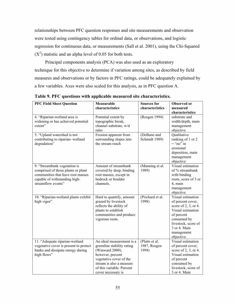
relationships between PFC question responses and site measurements and observation

were tested using contingency tables for ordinal data, or observations, and logistic

regression for continuous data, or measurements (Sall et al. 2001), using the Chi-Squared

(X2) statistic and an alpha level of 0.05 for both tests.

Principal components analysis (PCA) was also used as an exploratory

technique for this objective to determine if variation among sites, as described by field

measures and observations or by factors in PFC ratings, could be adequately explained by

a few variables. Axes were also scaled for this analysis, as in PFC question A.

Table 9. PFC questions with applicable measured site characteristics. PFC Field Sheet Question Measurable

characteristics Sources for characteristics

Observed or measured characteristics

4. “Riparian-wetland area is widening or has achieved potential extent”

Potential extent by topographic break, channel substrate, w/d ratio

(Rosgen 1994) substrate and width/depth, main management objective

5. “Upland watershed is not contributing to riparian- wetland degradation”

Erosion apparent from surrounding slopes into the stream reach

(DeBano and Schmidt 1989)

Qualitative ranking of 1 or 2 = “no” in erosional deposition, main management objective

9. “Streambank vegetation is comprised of those plants or plant communities that have root masses capable of withstanding high-streamflow events”

Amount of streambank covered by deep, binding root masses, except in bedrock or boulder channels.

(Manning et al. 1989)

Visual estimation of % streambank with binding roots, score of 3 or 4, main management objective

10. “Riparian-wetland plants exhibit high vigor”

Hard to quantify, amount grazed by livestock reflects the ability of plants to establish communities and produce vigorous roots.

(Prichard et al. 1998)

Visual estimation of percent cover, score of 2, 3, or 4. Visual estimation of percent consumed by livestock, score of 3 or 4. Main management objective.

11. “Adequate riparian-wetland vegetative cover is present to protect banks and dissipate energy during high flows”

An ideal measurement is a greenline stability rating (Winward 2000), however, percent vegetative cover of the stream is also a measure of this variable. Percent cover necessary is

(Platts et al. 1987, Rosgen 1994)

Visual estimation of percent cover, score of 2, 3, or 4. Visual estimation of percent consumed by livestock, score of 3 or 4. Main

55

determined by the channel and bank type.

management objective.

13. “Floodplain and channel characteristics are adequate to dissipate energy”

Measurement of sinuousity, w/d ratio, stream gradient

(Cowan 1956, Rosgen 1994)

W/d ratio and stream gradient.

56

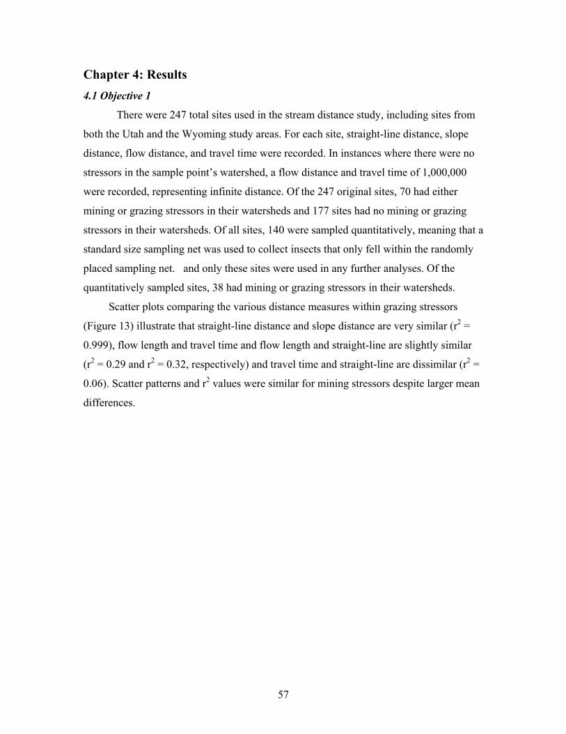
Chapter 4: Results 4.1 Objective 1

There were 247 total sites used in the stream distance study, including sites from

both the Utah and the Wyoming study areas. For each site, straight-line distance, slope

distance, flow distance, and travel time were recorded. In instances where there were no

stressors in the sample point’s watershed, a flow distance and travel time of 1,000,000

were recorded, representing infinite distance. Of the 247 original sites, 70 had either

mining or grazing stressors in their watersheds and 177 sites had no mining or grazing

stressors in their watersheds. Of all sites, 140 were sampled quantitatively, meaning that a

standard size sampling net was used to collect insects that only fell within the randomly

placed sampling net. and only these sites were used in any further analyses. Of the

quantitatively sampled sites, 38 had mining or grazing stressors in their watersheds.

Scatter plots comparing the various distance measures within grazing stressors

(Figure 13) illustrate that straight-line distance and slope distance are very similar (r2 =

0.999), flow length and travel time and flow length and straight-line are slightly similar

(r2 = 0.29 and r2 = 0.32, respectively) and travel time and straight-line are dissimilar (r2 =

0.06). Scatter patterns and r2 values were similar for mining stressors despite larger mean

differences.

57

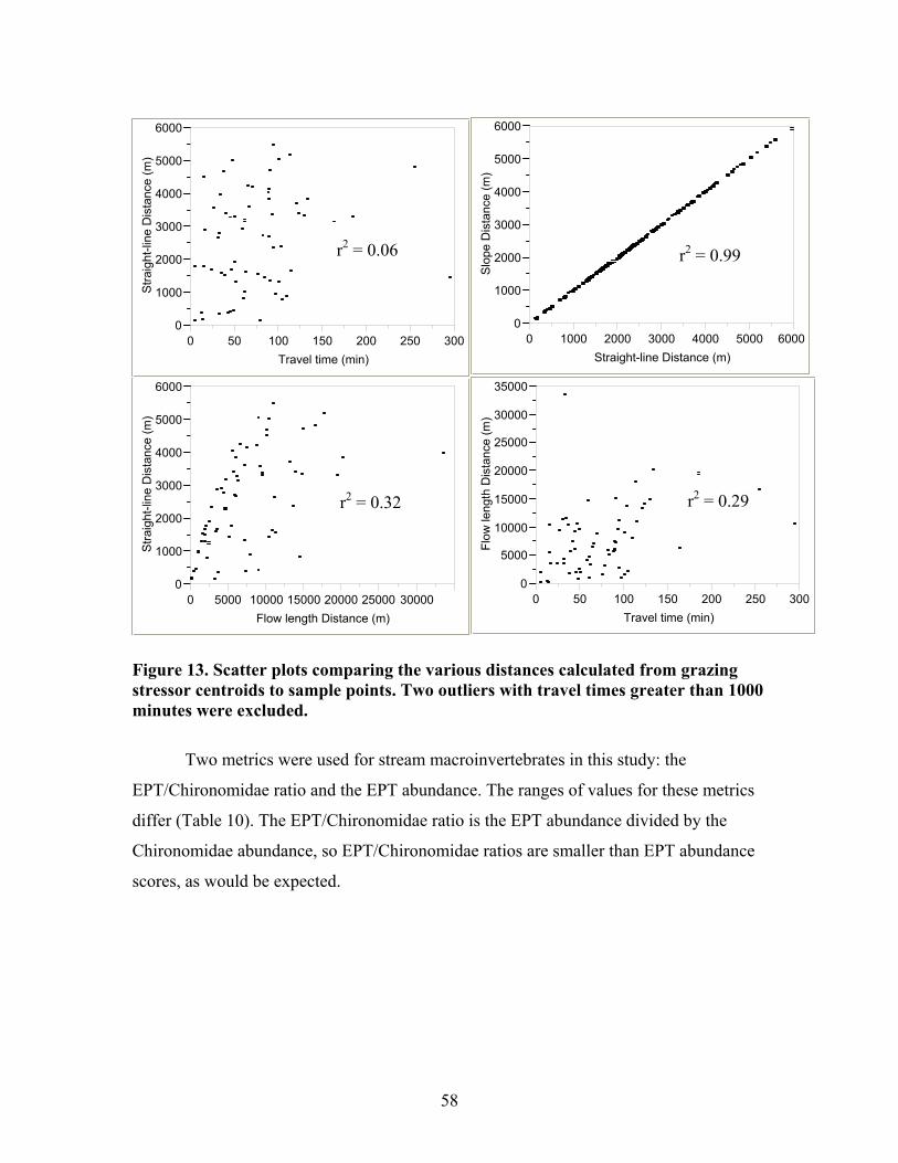
0

5000

10000

15000

20000

25000

30000

35000

Flow

leng

th D

ista

nce

(m)

0 50 100 150 200 250 300Travel time (min)

0

1000

2000

3000

4000

5000

6000S

traig

ht-li

ne D

ista

nce

(m)

0 50 100 150 200 250 300Travel time (min)

0

1000

2000

3000

4000

5000

6000

Slo

pe D

ista

nce

(m)

0 1000 2000 3000 4000 5000 6000Straight-line Distance (m)

r2 = 0.99 r2 = 0.06

0

1000

2000

3000

4000

5000

6000

Stra

ight

-line

Dis

tanc

e (m

)

0 5000 10000 15000 20000 25000 30000Flow length Distance (m)

r2 = 0.29 r2 = 0.32

Figure 13. Scatter plots comparing the various distances calculated from grazing stressor centroids to sample points. Two outliers with travel times greater than 1000 minutes were excluded.

Two metrics were used for stream macroinvertebrates in this study: the

EPT/Chironomidae ratio and the EPT abundance. The ranges of values for these metrics

differ (Table 10). The EPT/Chironomidae ratio is the EPT abundance divided by the

Chironomidae abundance, so EPT/Chironomidae ratios are smaller than EPT abundance

scores, as would be expected.

58

Table 10. Differences in mean and range of values for the macroinvertebrate metrics used in the stream distance study.

Metric Mean (both study areas) Maxium Minimum EPT 822 20957 0 EPT/Chir 5.15 247 0

A t-test was used to test for a difference in mean EPT/Chironomidae ratio and mean

EPT abundance between the sites with stressor centroids and the sites without stressor

centroids. A difference in means was expected between the two groups. There was no

statistically significant evidence (p > 0.10) that the mean EPT/Chironomidae ratio or

mean EPT abundance differed between sites with and sites without mining or grazing

stressor centroids in their watersheds. Furthermore, one-way ANOVAS were run to test

for differences in mean EPT/Chironomidae ratio in sampling method (Surber net, kick

net, plankton net, Hess net) and habitat (riffle, pool, pelagic, littoral, backwater, tinaja,

multiple habitats). There was no statistically significant evidence that the mean

EPT/Chironomidae ratio or EPT abundance differed between sampling techniques (p >

0.10) or habitats sampled (p > 0.10). A one-way ANOVA was also used to determine the

difference in mean EPT/Chironomidae ratio and EPT abundance between aquatic

ecoregions (Omernik 1987) and the same test was run for differences in means between

states. There was no statistically significant evidence that mean EPT/Chironomidae ratio

difference between ecoregions or states (p > 0.10). However, there was statistically

significant evidence that mean EPT abundance differed between ecoregions and states (p

< 0.0001, both tests). Significant differences in mean EPT abundance between ecoregions

was tested using Tukey’s HSD. Significant (< 0.05) differences occurred in all pairs of

ecoregions except the Middle Rockies and Wasatch and Uinta Mountains, and between

the Colorado Plateaus and the Wasatch and Uinta Mountains (Table 11).

59

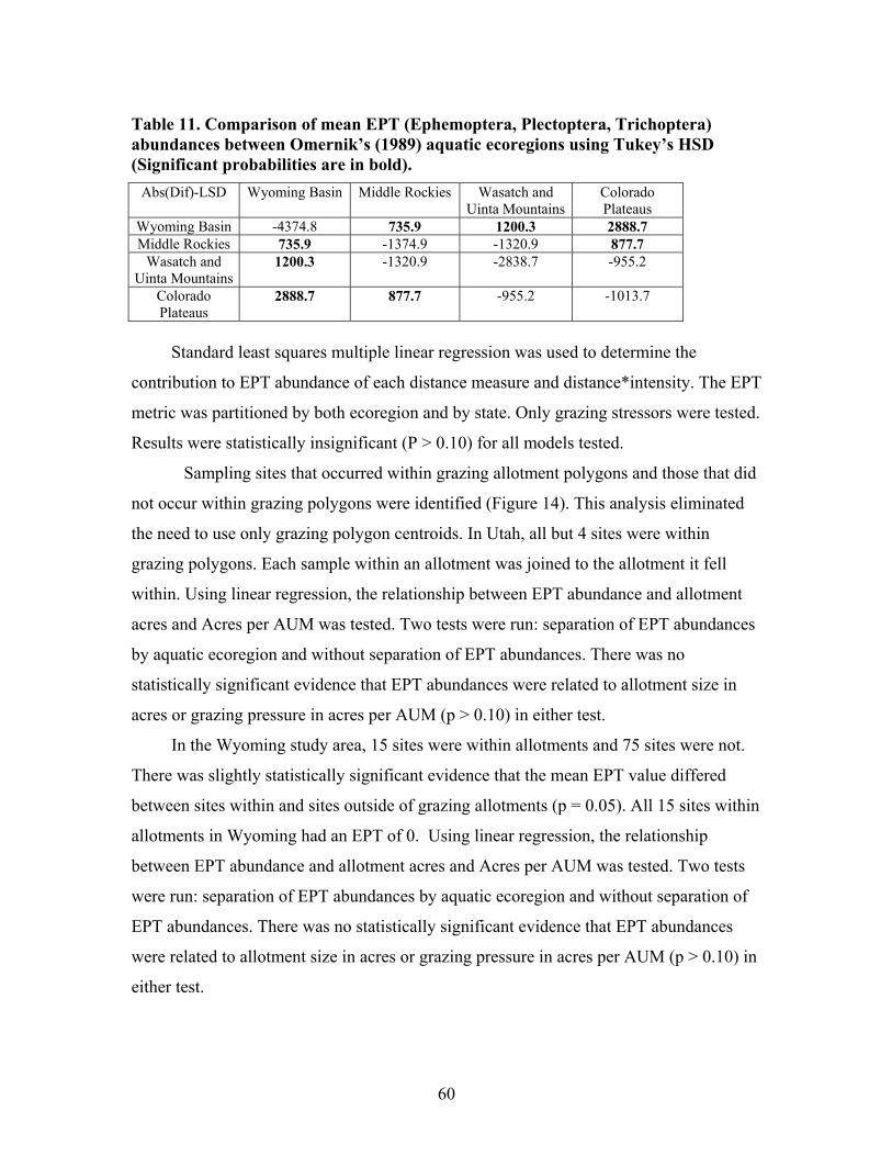
Table 11. Comparison of mean EPT (Ephemoptera, Plectoptera, Trichoptera) abundances between Omernik’s (1989) aquatic ecoregions using Tukey’s HSD (Significant probabilities are in bold).

Abs(Dif)-LSD Wyoming Basin Middle Rockies Wasatch and Uinta Mountains

Colorado Plateaus

Wyoming Basin -4374.8 735.9 1200.3 2888.7 Middle Rockies 735.9 -1374.9 -1320.9 877.7

Wasatch and Uinta Mountains

1200.3 -1320.9 -2838.7 -955.2

Colorado Plateaus

2888.7 877.7 -955.2 -1013.7

Standard least squares multiple linear regression was used to determine the

contribution to EPT abundance of each distance measure and distance*intensity. The EPT

metric was partitioned by both ecoregion and by state. Only grazing stressors were tested.

Results were statistically insignificant (P > 0.10) for all models tested.

Sampling sites that occurred within grazing allotment polygons and those that did

not occur within grazing polygons were identified (Figure 14). This analysis eliminated

the need to use only grazing polygon centroids. In Utah, all but 4 sites were within

grazing polygons. Each sample within an allotment was joined to the allotment it fell

within. Using linear regression, the relationship between EPT abundance and allotment

acres and Acres per AUM was tested. Two tests were run: separation of EPT abundances

by aquatic ecoregion and without separation of EPT abundances. There was no

statistically significant evidence that EPT abundances were related to allotment size in

acres or grazing pressure in acres per AUM (p > 0.10) in either test.

In the Wyoming study area, 15 sites were within allotments and 75 sites were not.

There was slightly statistically significant evidence that the mean EPT value differed

between sites within and sites outside of grazing allotments (p = 0.05). All 15 sites within

allotments in Wyoming had an EPT of 0. Using linear regression, the relationship

between EPT abundance and allotment acres and Acres per AUM was tested. Two tests

were run: separation of EPT abundances by aquatic ecoregion and without separation of

EPT abundances. There was no statistically significant evidence that EPT abundances

were related to allotment size in acres or grazing pressure in acres per AUM (p > 0.10) in

either test.

60

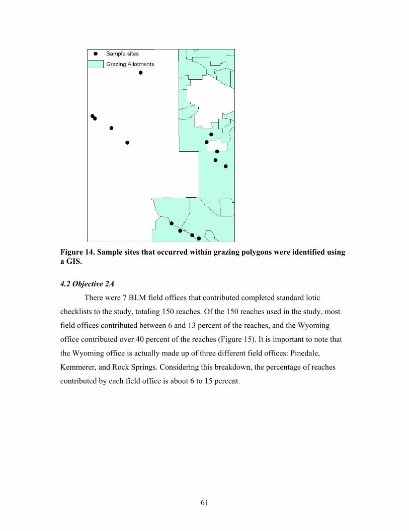
Figure 14. Sample sites that occurred within grazing polygons were identified using a GIS.

4.2 Objective 2A

There were 7 BLM field offices that contributed completed standard lotic

checklists to the study, totaling 150 reaches. Of the 150 reaches used in the study, most

field offices contributed between 6 and 13 percent of the reaches, and the Wyoming

office contributed over 40 percent of the reaches (Figure 15). It is important to note that

the Wyoming office is actually made up of three different field offices: Pinedale,

Kemmerer, and Rock Springs. Considering this breakdown, the percentage of reaches

contributed by each field office is about 6 to 15 percent.

61

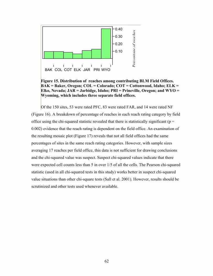
0.10

0.20

0.30

0.40

BAK COL COT ELK JAR PRI WYO

Perc

enta

geof

reac

hes

Figure 15. DistriBAK = Baker, OElko, Nevada; JAWyoming, which

Of the 150 sites, 5

(Figure 16). A breakdow

office using the chi-squ

0.002) evidence that the

the resulting mosaic plo

percentages of sites in t

averaging 17 reaches pe

and the chi-squared val

were expected cell coun

statistic (used in all chi-

value situations than ot

scrutinized and other te

bution of reaches among contributing BLM Field Offices. regon; COL = Colorado; COT = Cottonwood, Idaho; ELK = R = Jarbidge, Idaho; PRI = Prineville, Oregon; and WYO =

includes three separate field offices.

3 were rated PFC, 83 were rated FAR, and 14 were rated NF

n of percentage of reaches in each reach rating category by field

ared statistic revealed that there is statistically significant (p =

reach rating is dependent on the field office. An examination of

t (Figure 17) reveals that not all field offices had the same

he same reach rating categories. However, with sample sizes

r field office, this data is not sufficient for drawing conclusions

ue was suspect. Suspect chi-squared values indicate that there

ts less than 5 in over 1/5 of all the cells. The Pearson chi-squared

squared tests in this study) works better in suspect chi-squared

her chi-square tests (Sall et al. 2001). However, results should be

sts used whenever available.

62

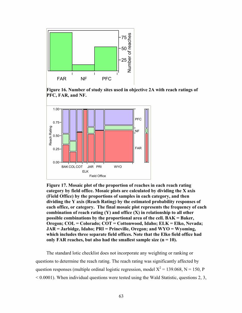
25

50

75

Num

ber o

f rea

ches

FAR NF PFC

Figure 16. Number of study sites used in objective 2A with reach ratings of PFC, FAR, and NF.

Rea

ch R

atin

g

0.00

0.25

0.50

0.75

1.00

BAK COLCOTELK

JAR PRI WYO

Field Office

FAR

NF

PFC

Figure 17. Mosaic plot of the proportion of reaches in each reach rating category by field office. Mosaic plots are calculated by dividing the X axis (Field Office) by the proportions of samples in each category, and then dividing the Y axis (Reach Rating) by the estimated probability responses of each office, or category. The final mosaic plot represents the frequency of each combination of reach rating (Y) and office (X) in relationship to all other possible combinations by the proportional area of the cell. BAK = Baker, Oregon; COL = Colorado; COT = Cottonwood, Idaho; ELK = Elko, Nevada; JAR = Jarbidge, Idaho; PRI = Prineville, Oregon; and WYO = Wyoming, which includes three separate field offices. Note that the Elko field office had only FAR reaches, but also had the smallest sample size (n = 10).

The standard lotic checklist does not incorporate any weighting or ranking or

questions to determine the reach rating. The reach rating was significantly affected by

question responses (multiple ordinal logistic regression, model X2 = 139.068, N = 150, P

< 0.0001). When individual questions were tested using the Wald Statistic, questions 2, 3,

63

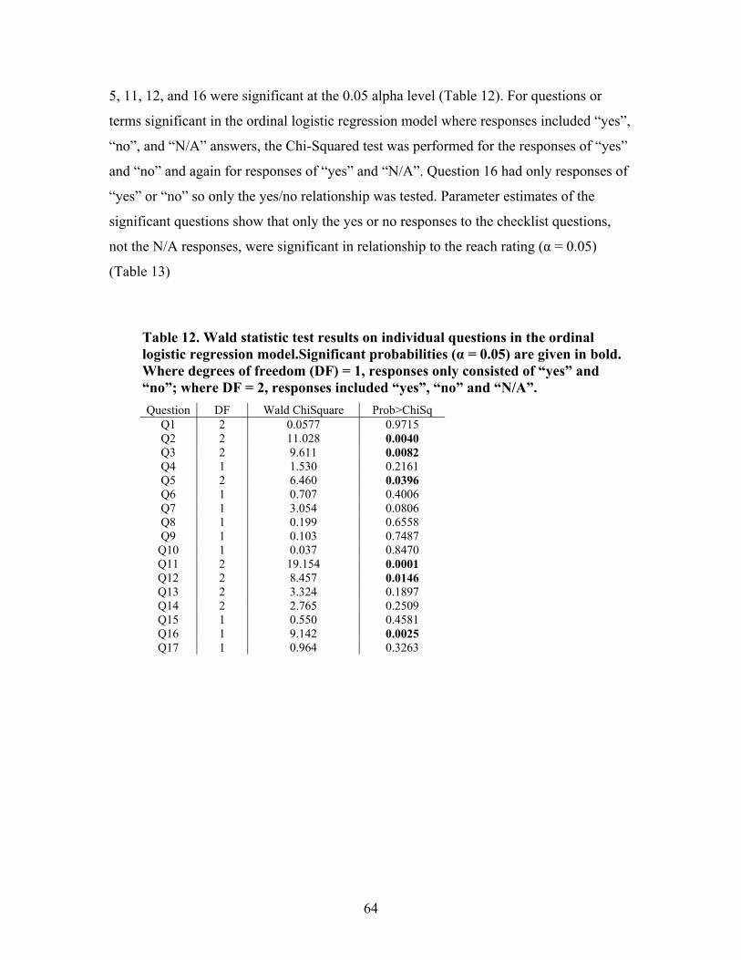
5, 11, 12, and 16 were significant at the 0.05 alpha level (Table 12). For questions or

terms significant in the ordinal logistic regression model where responses included “yes”,

“no”, and “N/A” answers, the Chi-Squared test was performed for the responses of “yes”

and “no” and again for responses of “yes” and “N/A”. Question 16 had only responses of

“yes” or “no” so only the yes/no relationship was tested. Parameter estimates of the

significant questions show that only the yes or no responses to the checklist questions,

not the N/A responses, were significant in relationship to the reach rating (α = 0.05)

(Table 13)

Table 12. Wald statistic test results on individual questions in the ordinal logistic regression model.Significant probabilities (α = 0.05) are given in bold. Where degrees of freedom (DF) = 1, responses only consisted of “yes” and “no”; where DF = 2, responses included “yes”, “no” and “N/A”. Question DF Wald ChiSquare Prob>ChiSq

Q1 2 0.0577 0.9715 Q2 2 11.028 0.0040 Q3 2 9.611 0.0082 Q4 1 1.530 0.2161 Q5 2 6.460 0.0396 Q6 1 0.707 0.4006 Q7 1 3.054 0.0806 Q8 1 0.199 0.6558 Q9 1 0.103 0.7487

Q10 1 0.037 0.8470 Q11 2 19.154 0.0001 Q12 2 8.457 0.0146 Q13 2 3.324 0.1897 Q14 2 2.765 0.2509 Q15 1 0.550 0.4581 Q16 1 9.142 0.0025 Q17 1 0.964 0.3263

64

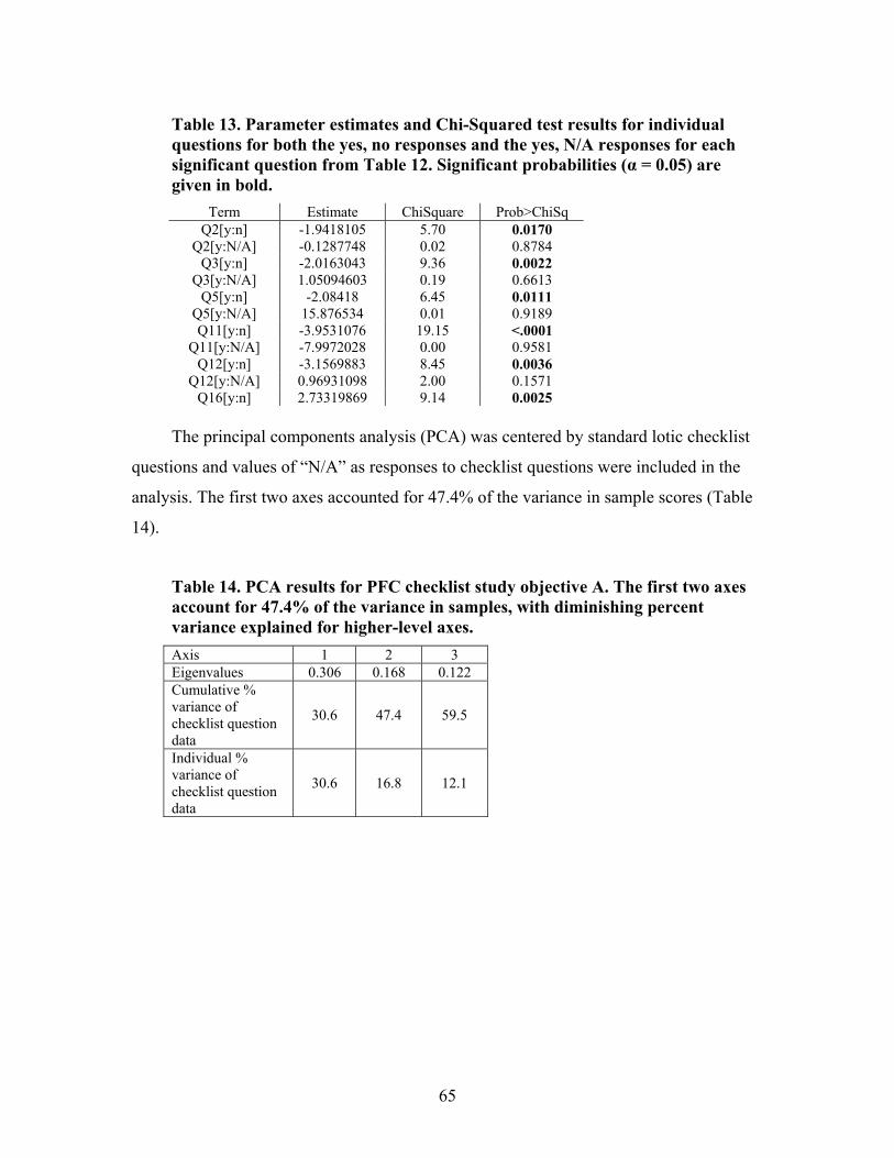
Table 13. Parameter estimates and Chi-Squared test results for individual questions for both the yes, no responses and the yes, N/A responses for each significant question from Table 12. Significant probabilities (α = 0.05) are given in bold.

Term Estimate ChiSquare Prob>ChiSq Q2[y:n] -1.9418105 5.70 0.0170

Q2[y:N/A] -0.1287748 0.02 0.8784 Q3[y:n] -2.0163043 9.36 0.0022

Q3[y:N/A] 1.05094603 0.19 0.6613 Q5[y:n] -2.08418 6.45 0.0111

Q5[y:N/A] 15.876534 0.01 0.9189 Q11[y:n] -3.9531076 19.15 <.0001

Q11[y:N/A] -7.9972028 0.00 0.9581 Q12[y:n] -3.1569883 8.45 0.0036

Q12[y:N/A] 0.96931098 2.00 0.1571 Q16[y:n] 2.73319869 9.14 0.0025

The principal components analysis (PCA) was centered by standard lotic checklist

questions and values of “N/A” as responses to checklist questions were included in the

analysis. The first two axes accounted for 47.4% of the variance in sample scores (Table

14).

Table 14. PCA results for PFC checklist study objective A. The first two axes account for 47.4% of the variance in samples, with diminishing percent variance explained for higher-level axes. Axis 1 2 3 Eigenvalues 0.306 0.168 0.122 Cumulative % variance of checklist question data

30.6 47.4 59.5

Individual % variance of checklist question data

30.6 16.8 12.1

65

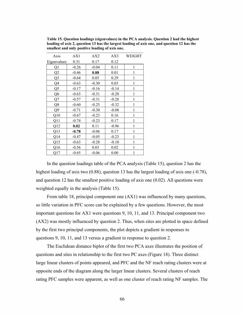
Table 15. Question loadings (eigenvalues) in the PCA analysis. Question 2 had the highest loading of axis 2, question 13 has the largest loading of axis one, and question 12 has the smallest and only positive loading of axis one.

Axis AX1 AX2 AX3 WEIGHTEigenvalues 0.31 0.17 0.12

Q1 -0.26 -0.04 0.11 1 Q2 -0.46 0.88 0.01 1 Q3 -0.64 0.05 0.29 1 Q4 -0.63 -0.30 0.03 1 Q5 -0.17 -0.16 -0.14 1 Q6 -0.63 -0.31 -0.20 1 Q7 -0.57 -0.31 -0.28 1 Q8 -0.60 -0.25 -0.32 1 Q9 -0.71 -0.30 -0.08 1

Q10 -0.67 -0.23 0.16 1 Q11 -0.74 -0.23 0.17 1 Q12 0.02 0.11 -0.96 1 Q13 -0.78 -0.06 0.17 1 Q14 -0.47 -0.05 -0.23 1 Q15 -0.63 -0.28 -0.10 1 Q16 -0.56 0.03 0.02 1 Q17 -0.65 -0.06 0.00 1

In the question loadings table of the PCA analysis (Table 15), question 2 has the

highest loading of axis two (0.88), question 13 has the largest loading of axis one (-0.78),

and question 12 has the smallest positive loading of axis one (0.02). All questions were

weighted equally in the analysis (Table 15).

From table 18, principal component one (AX1) was influenced by many questions,

so little variation in PFC score can be explained by a few questions. However, the most

important questions for AX1 were questions 9, 10, 11, and 13. Principal component two

(AX2) was mostly influenced by question 2. Thus, when sites are plotted in space defined

by the first two principal components, the plot depicts a gradient in responses to

questions 9, 10, 11, and 13 versus a gradient in response to question 2.

The Euclidean distance biplot of the first two PCA axes illustrates the position of

questions and sites in relationship to the first two PC axes (Figure 18). Three distinct

large linear clusters of points appeared, and PFC and the NF reach rating clusters were at

opposite ends of the diagram along the larger linear clusters. Several clusters of reach

rating PFC samples were apparent, as well as one cluster of reach rating NF samples. The

66

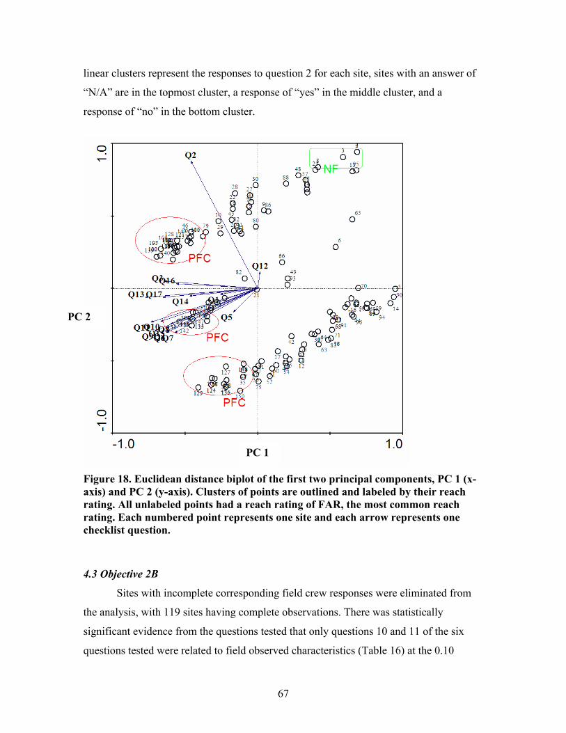
linear clusters represent the responses to question 2 for each site, sites with an answer of

“N/A” are in the topmost cluster, a response of “yes” in the middle cluster, and a

response of “no” in the bottom cluster.

PC 2

PC 1

Figure 18. Euclidean distance biplot of the first two principal components, PC 1 (x-axis) and PC 2 (y-axis). Clusters of points are outlined and labeled by their reach rating. All unlabeled points had a reach rating of FAR, the most common reach rating. Each numbered point represents one site and each arrow represents one checklist question. 4.3 Objective 2B

Sites with incomplete corresponding field crew responses were eliminated from

the analysis, with 119 sites having complete observations. There was statistically

significant evidence from the questions tested that only questions 10 and 11 of the six

questions tested were related to field observed characteristics (Table 16) at the 0.10

67

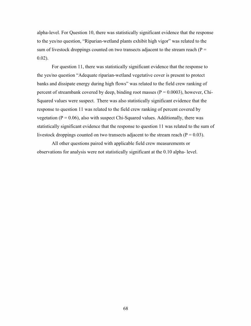
alpha-level. For Question 10, there was statistically significant evidence that the response

to the yes/no question, “Riparian-wetland plants exhibit high vigor” was related to the

sum of livestock droppings counted on two transects adjacent to the stream reach (P =

0.02).

For question 11, there was statistically significant evidence that the response to

the yes/no question “Adequate riparian-wetland vegetative cover is present to protect

banks and dissipate energy during high flows” was related to the field crew ranking of

percent of streambank covered by deep, binding root masses (P = 0.0003), however, Chi-

Squared values were suspect. There was also statistically significant evidence that the

response to question 11 was related to the field crew ranking of percent covered by

vegetation (P = 0.06), also with suspect Chi-Squared values. Additionally, there was

statistically significant evidence that the response to question 11 was related to the sum of

livestock droppings counted on two transects adjacent to the stream reach (P = 0.03).

All other questions paired with applicable field crew measurements or

observations for analysis were not statistically significant at the 0.10 alpha- level.

68

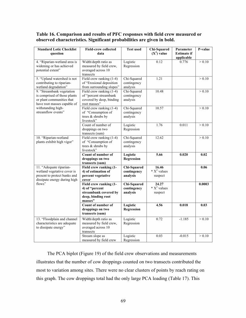
Table 16. Comparison and results of PFC responses with field crew measured or observed characteristics. Significant probabilities are given in bold.

Standard Lotic Checklist question

Field-crew collected data

Test used Chi-Squared (X2) value

Parameter Estimate if applicable

P-value

4. “Riparian-wetland area is widening or has achieved potential extent”

Width/depth ratio as measured by field crew, averaged across 10 transects

Logistic Regression

0.12 0.776 > 0.10

5. “Upland watershed is not contributing to riparian- wetland degradation”

Field crew ranking (1-4) of “Erosional deposition from surrounding slopes”

Chi-Squared contingency analysis

1.21 > 0.10

Field crew ranking (1-4) of “percent streambank covered by deep, binding root masses”

Chi-Squared contingency analysis

10.48 > 0.10

Field crew ranking (1-4) of “Consumption of trees & shrubs by livestock”

Chi-Squared contingency analysis

10.57 > 0.10

9. “Streambank vegetation is comprised of those plants or plant communities that have root masses capable of withstanding high-streamflow events”

Count of number of droppings on two transects (sum)

Logistic Regression

1.76 0.011 > 0.10

Field crew ranking (1-4) of “Consumption of trees & shrubs by livestock”

Chi-Squared contingency analysis

12.62 > 0.10 10. “Riparian-wetland plants exhibit high vigor”

Count of number of droppings on two transects (sum)

Logistic Regression

5.66 0.020 0.02

Field crew ranking (1-4) of estimation of percent vegetative cover

Chi-Squared contingency analysis

16.46 * X2 values

suspect

0.06

Field crew ranking (1-4) of “percent streambank covered by deep, binding root masses”

Chi-Squared contingency analysis

24.27 * X2 values

suspect

0.0003

11. “Adequate riparian-wetland vegetative cover is present to protect banks and dissipate energy during high flows”

Count of number of droppings on two transects (sum)

Logistic Regression

4.56 0.018 0.03

Width/depth ratio as measured by field crew, averaged across 10 transects

Logistic Regression

0.72 -1.185 > 0.10 13. “Floodplain and channel characteristics are adequate to dissipate energy”

Stream slope as measured by field crew

Logistic Regression

0.03 -0.015 > 0.10

The PCA biplot (Figure 19) of the field crew observations and measurements

illustrates that the number of cow droppings counted on two transects contributed the

most to variation among sites. There were no clear clusters of points by reach rating on

this graph. The cow droppings total had the only large PCA loading (Table 17). This

69

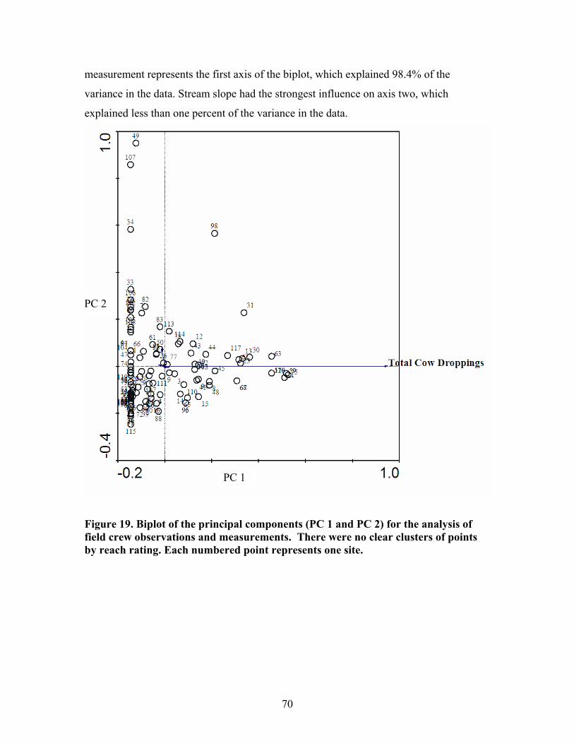
measurement represents the first axis of the biplot, which explained 98.4% of the

variance in the data. Stream slope had the strongest influence on axis two, which

explained less than one percent of the variance in the data.

PC 2

PC 1

Figure 19. Biplot of the principal components (PC 1 and PC 2) for the analysis of field crew observations and measurements. There were no clear clusters of points by reach rating. Each numbered point represents one site.

70

Table 17. Principal Components loadings of the PCA analysis of field-crew measured characteristics.

Axis AX1 AX2 AX3 WEIGHTEigenvalue 0.984 0.0072 0.0038

Vegetative Cover -0.0408 0.012 -0.0989 1 Erosion -0.0204 0.026 -0.0552 1

Consumption -0.0811 0.0199 -0.0596 1 Incisement 0.0061 0.0205 -0.01 1 Root Mass -0.0126 0.0097 -0.1157 1 Cow total 2.8039 0.0042 -0.0038 1

Stream Slope -0.0383 0.2365 0.0218 1 Width/Depth ratio -0.0009 -0.0021 0.0005 1

71

Chapter 5: Discussion 5.1 Objective 1

There was no statistically significant evidence that the mean EPT abundances or

EPT/Chironomidae ratios of sites with stressor centroids in their watersheds and sites

without stressor centroids in their watersheds differed (p > 0.10).

A large body of literature supports the idea that landscape stressors in the

contributing area to a sample point will affect the riparian condition, and ultimately, biota

composition at that site (Beasley and Kneale 2002, García - Criado et al. 1999, Kauffman

and Kreuger 1984, Maret et al. 2001, Marqués et al. 2003, Townsend et al. 1997).

However, the relationships between biotic community structure and landscape stressors

are extremely complex (Hawkins and Vinson 2000, Muhar and Jungwirth 1998). There

also exists a wide range of biotic metrics for the researcher to test, with each metric

having strengths and weaknesses in the amounts and types of stress measured by the

biotic signals (Grigorovich and Angermeier 2004). Additionally, some sites are

inherently more sensitive to impacts than others, particularly livestock grazing impacts

(Chaney et al. 1993).

The lack of separation between sites with stressor centroids and sites without

stressor centroids may indicate that using stressor centroids for polygon stressors is not

relevant. It may potentially indicate that BLM management techniques of land use and

riparian areas are effective in mitigating the effects of grazing and mining on stream

communities. However, no statistical inference can be made in direct relationship to the

BLM’s management practices, because not all study sites fell on BLM lands. It is

important to note that all stressor data were cataloged by the BLM, which may mean that

some stressors on non-BLM land were omitted from the study.

There was slightly statistically significant evidence that in the Wyoming study area,

the mean EPT value differed between sites within and sites outside of grazing allotments

(p = 0.05) without the use of centroids. It is interesting to note that all sites within

allotments had an EPT of 0. However, using linear regression, there was no statistically

significant relationship between EPT and allotment acres or acres/AUM (p > 0.10). This

may demonstrate that acres per AUM is unsuitable as an indicator of grazing pressure.

72

There was insufficient statistical power to detect a difference, and an increased sample

size was needed, particularly of sites within allotments in the Wyoming study area.

There was also statistically significant evidence that the mean EPT abundances

differed both between aquatic ecoregions and between states (p < 0.001, both tests). This

may further the case that the presence or absence of stressor centroids within sample

watersheds is not relevant in partitioning biotic variance.

The biological significance of the four distance measurements in characterizing

stressor impacts could not be quantified using multiple linear regression. While travel

time and flow length distances appear logically superior to straight-line and slope

distances, this study was not able to assess the biological significance of these measures.

The mean differences in distances measured using slope distance and flow length (5197

meters for grazing and 14951 meters for mining mean difference) indicate some degree

of difference in the distance measurements. Grazing allotments occurred throughout the

watersheds, and mining leases occurred in clusters, leading to a difference in mean

distances between the two stressors. Additionally, when comparing distance measures to

one another using linear regression, the greatest difference occurred between straight-line

and travel time. There was almost no difference between straight-line and slope distance,

and nearly equal differences between straight-line and flow length, and flow length and

travel time. The lack of correlation (r2=0.06) between straight-line distance, which is the

simplest measure tested and also the least hydrologically relevant; and travel time, which

is the most detailed distance measure tested and the most hydrologically relevant of those

studied, may indicate that these distances and their biological relevance warrant further

study.

The results of this study illustrate the need for a more controlled study approach. A

controlled paired watershed study of the potential relationship of distance (including

travel time) with biotic signals would also enable the researcher to compare travel time

with other distances without the hindrance of trying to directly compare two distinct units

of measurement (time and distance). Additionally, research should take Omernik’s (1989)

aquatic ecoregions for partitioning regional variances in EPT abundance.

Further study is necessary, with a more focused and controlled study approach.

This study, in keeping with the goals of the AILC, attempted to use a large study area and

73

also used pre-existing data and locations. Sample locations and times of collection were

already present when this study began. The study was constrained to already existing

data. When measuring landscape stressors as diverse and dynamic as cattle grazing,

which can change from month to month, a smaller temporal scale, such as monthtly

measurements of both grazing pressure and macroinvertebrate communities, may prove

helpful. Cattle grazing impacts can also be extremely localized (Grigorovich and

Angermeier 2004) so a focused spatial approach may also be helpful. Focused temporal

testing of sites in a limited spatial area may yield useful data.

5.2 Objective 2A

Checklist questions 2, 3, 5, 11, 12, and 16 significantly affected the reach rating in

the multiple logistic regression analysis (MLR).

From the PCA biplot (Figure 18), questions 3 and 16 are similar, indicated by the

small angle of separation between the two arrows on the biplot. In the PFC assessment,

questions 3 and 16 are not in the same groups of questions on the standard lotic checklist.

Question 3 is in the erosion/deposition group and question 16 is in the hydrology group.

Question 3, “Sinuosity, width/depth ratio, and gradient are in balance with the landscape

setting” is designed to assess the dissipation of energy through the reach, assuming that

when the reach is not in balance with its setting, rapid erosion will occur due to less

dissipation of energy (Prichard et al. 1998). Question 16, “System is vertically stable” is

designed to assess if the streambed is lowering rapidly as a result of erosion (Prichard et

al. 1998). Both of these questions assess the stability and dissipation of energy through a

reach. Question 3 addresses a broad view of reach stability and question 16 addresses an

individual effect of reach stability. Question 3 also has a longer arrow than question 16 in

the PCA diagram (Figure 18) indicating a stronger relationship with the data. It may be

that question 3 is sufficient to assess reach stability for the reach rating.

Question 5, “Upland watershed is not contributing to riparian- wetland

degradation,” had a p-value of 0.04 in the MLR. From a mosaic plot of the responses to

question 5, it appears that there is little separation between FAR and NF with yes/no

answers as would be expected (Figure 20), as the height of the cells in the mosaic plot for

“no” and “yes” answers are similar. Additionally, in the PCA biplot (Figure 18), question

74

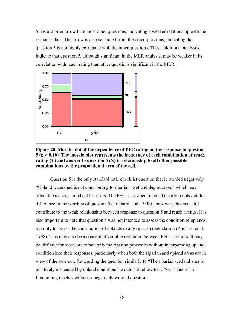
5 has a shorter arrow than most other questions, indicating a weaker relationship with the

response data. The arrow is also separated from the other questions, indicating that

question 5 is not highly correlated with the other questions. These additional analyses

indicate that question 5, although significant in the MLR analysis, may be weaker in its

correlation with reach rating than other questions significant in the MLR.

Rea

ch R

atin

g

0.00

0.25

0.50

0.75

1.00

2

FAR

NF

PFC

s

Figure 205 (p > 0.1rating (Ycombinat

Qu

“Upland w

affect the

difference

contribute

also impor

but only to

1998). Th

be difficul

condition

view of th

positively

functionin

0no

Q5

. Mosaic plot of t0). The mosaic pl) and answer to qions by the propo

estion 5 is the on

atershed is not co

response of check

in the wording of

to the weak relati

tant to note that q

assess the contri

is may also be a c

t for assessors to

into their response

e assessor. Re-wo

influenced by upl

g reaches without

1ye

he dependencot representsuestion 5 (X)rtional area

ly standard lot

ntributing to r

list users. The

question 5 (P

onship betwee

uestion 5 was

bution of upla

oncept of varia

rate only the r

s, particularly

rding the ques

and condition

a negatively w

e of PFC rating on the response to question

the frequency of each combination of reach in relationship to all other possible of the cell.

ic checklist question that is worded negatively

iparian- wetland degradation,” which may

PFC assessment manual clearly points out this

richard et al. 1998) , however, this may still

n response to question 5 and reach ratings. It is

not intended to assess the condition of uplands,

nds to any riparian degradation (Prichard et al.

ble definition between PFC assessors. It may

iparian processes without incorporating upland

when both the riparian and upland areas are in

tion similarly to “The riparian-wetland area is

s” would still allow for a “yes” answer in

orded question.

75

There were two questions significant in the MLR that had “N/A” response rates of

over 20 percent. Question 2, “Active/stable beaver dams” and question 12, “Plant

communities in the riparian area are an adequate source of coarse and/or large woody

debris” both had high levels of “N/A” responses. However, both of these questions were

statistically significant at the 0.05 alpha level in the MLR. Additionally, in the PCA

biplot (Figure 18), questions 2 and 12 were both separated from the majority of the

checklist questions as indicated by the angles between the arrows on the diagram. This

indicates low correlation with other checklist questions, which may suggest that these

questions assess unique characteristics of the reaches. In the PCA diagram, question 2 has

the longest arrow of any checklist question, indicating a very strong relationship to the

response data, and question 12 has the shortest arrow of any checklist question, indicating

the weakest relationship to the response data. It should also be noted that question 2 is the

only checklist question with more “no” and “N/A” than “yes” responses. All other

questions had more “yes” than “no” responses. This difference may affect the importance

of this question in the final reach rating dramatically and may contribute to its

overwhelming dominance in the PCA biplot (Figure 18).

From the high levels of N/A response rates, it appears that these questions may not

be universally applicable to diverse western rangelands. When applicable, they may be

helpful in assessing reach rating, as illustrated by the MLR and PCA analysis results, but

over 20 percent of the time, they are not applicable or present. Question 2, “Where

beaver dams are present, they are active and stable” is only intended to be answered with

a “yes” or “no” where beaver dams are present, and should be answered “N/A” where

they are not present (Prichard et al. 1998). The high level of “N/A” responses to the

question indicates that many sites do not have beaver dams. However, the question does

appear to have a strong, unique relationship to the response data and appears to

overwhelm the presence of all other questions when beaver dams are present (Figure 18),

affirmed by its dominant loading of the second PCA axis, while its universal applicability

to all sites appears weak. The PFC assessment manual acknowledges that question 12,

“Plant communities in the riparian area are an adequate source of coarse and/or large

woody debris,” will have high levels of “N/A” responses in the west. Coarse woody

debris is only important to the functioning of those stream reaches in forested areas, and

76

the majority of BLM western rangelands are not forested. It appears from the PCA

analysis that question 12 has a unique but weak relationship with the response data.

Question 11 was significant in the MLR but was not correlated with any other

significant questions and did not have high levels of N/A responses. Question 11,

“adequate riparian-wetland cover is present to protect banks and dissipate energy during

high flows, ” is part of the vegetation group of questions. Of all the checklist questions

pertaining to vegetation (Appendix A), question 11 appears to be the most general and

directly related to the overall goal of the PFC assessment. For a reach to receive a rating

of PFC, it must have the ability to withstand and recover from high flow events. The

overall goal of the PFC assessment is to assess resilience and dissipation of flows.

Question 11 directly addresses this issue for the vegetation segment of the assessment,

and this may be why question 11 is not correlated with any other significant questions,

significantly affects the reach ratings, and has one of the strongest relationships with the

data of any checklist question as shown in the PCA biplot (Figure 18). Question 11

appears to be a vital facet of the PFC assessment.

Questions 1, 4, 6, 7, 8, 9, 10, 13, 14, 15, and 17 did not significantly affect reach

rating at the 0.05 alpha level in the MLR analysis. It also appears from the PCA biplot

(Figure 18) that all these questions are highly correlated with each other or with other

significant questions. This may indicate a level of redundancy in the reach rating

resulting from the question responses, or it may indicate that assessors are not taking

these questions into account when assigning the final reach ratings. It was not possible

with the data available for this study to determine if these results were due to redundancy

or assessor use of the checklist in determining reach rating. The inclusion of a ranking,

addition, or weighting system based on the current standard lotic checklist questions may

address this issue by allowing assessors to take all checklist questions into account when

assigning the reach ratings. A weighting system is already in use by the Idaho Falls BLM

field office for a protocol that uses slightly different assessment questions, but the same

principle could be applied to the PFC assessment.

5.3 Objective 2B

Standard lotic checklist questions 10 and 11 were found be statistically related to

applicable field measured and observed characteristics.

77

Question 10, “Riparian plants exhibit high vigor,” was significantly related at the

0.10 alpha-level to the sum of livestock droppings counted along two transects, as was

question 11, “Adequate riparian-wetland vegetative cover is present to protect banks and

dissipate energy during high flows.” The parameter estimates for both questions were

small and positive numbers (Q10 = 0.020, Q 11 = 0.018), indicating that as the number of

cow droppings counted increases, the probability of question 10 or question 11 receiving

an answer of “no” also increases, but at a small rate of change. Livestock grazing is

known to reduce riparian vegetative cover through direct removal and trampling

(Kauffman and Kreuger 1984). It is logical that indicators of livestock presence, damage,

and consumption of vegetation would statistically correlate with riparian plant vigor and

amount of cover. This correlation may indicate that both checklist questions 10 and11 are

effective as binary responses within the PFC assessment to assess riparian damage due to

livestock presence and livestock removal. It may also indicate these questions are truly

applicable to diverse western rangelands.

For question 11, there was statistically significant evidence that the response to

“Adequate riparian-wetland vegetative cover is present to protect banks and dissipate

energy during high flows” was related to the field crew ranking of percent of streambank

covered by deep, binding root masses. There was also statistically significant evidence

that question 11 was related to the field crew estimation of percent vegetative cover in the

riparian area (ranked 1-4). This indicates an agreement between PFC assessors and the

independent field crew on the observation of vegetative cover. This may indicate that the

streambank coverage for this checklist question is related to both the amount and type of

vegetation within the reach, although the PFC assessment manual explains that this

question is designed to assess only the amount of vegetation (Prichard et al. 1998). This

relationship may also indicate that a binary response is sufficient to represent the amount

of vegetation present, when compared to a four-category response used by the field crew.

Additionally, the relationship between these two sets of observations may indicate that

adequate riparian cover is a repeatable, easily observable, and universal stream reach

characteristic.

It is important to note that the two contingency table analyses on question 11 had

suspect chi-squared values. This may indicate that the results are unstable. However,

78

there is statistically significant evidence that both question 10 and 11 are related to the

count of cow droppings, tested by logistic regression, and chi-squared values were not

suspect for these analyses.

Of the PFC questions with applicable field crew measured or observed stream reach

characteristics, four of the six tested questions had no statistically significant relationship

with field crew observations. There are several potential reasons for lack of correlation

with these responses, including design of the study, design of field crew measurements,

lack of regionalization, temporal differences between PFC and field crew observations,

small sample size, and potential problems inherent in the PFC process.

The study design may not have accounted for all possible combinations of field

crew measurements and PFC responses. Potential relationships were only explored when

logical relationships between the PFC question of field measurement could be justified

using the current knowledge base (Table 9) and description of techniques in the PFC

assessment field manual (Prichard et al. 1998). Additionally, field crew measured and

observed characteristics were not specifically designed for this study. The field crew

measurements and observations were designed previous to this study as part of a more

detailed macroinvertebrate study, and represented the only known data source sufficient

to meet needs for this objective. If field crew observations had been specifically tailored

to measure each aspect of the PFC assessment at the same sites, all 17 questions could

have been studied in greater detail.

Some of the lack of statistical relationship between the two protocols may have

been due to a need for regionalization of certain characteristics. For example, a stream

gradient of 2% may have been considered “in balance” in response to question 3 in a

mountainous area, but could be considered “out of balance” in an area with more gentle

topography. Regionalization by ecoregion, topographic relief, or other large-scale

characteristics may have resulted in more statistically significant relationships. However,

in this study, regionalization would have resulted in sample sizes far too small for

statistical analysis of these questions with the currently available data. A larger sample

size would be necessary for an analysis of this type.

Additionally, the temporal differences between the year of PFC observation and

field crew measurement may have been a factor. The average time in years between PFC

79

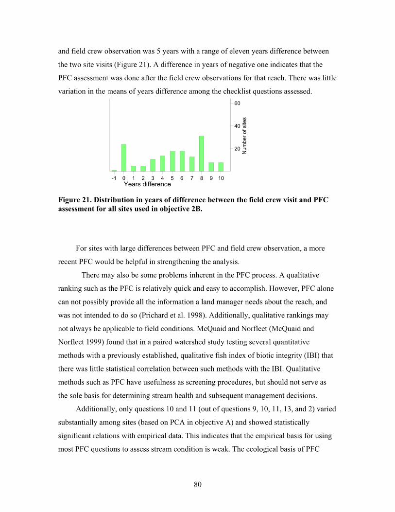
and field crew observation was 5 years with a range of eleven years difference between

the two site visits (Figure 21). A difference in years of negative one indicates that the

PFC assessment was done after the field crew observations for that reach. There was little

variation in the means of years difference among the checklist questions assessed.

20

40

60

Num

ber o

f site

s

-1 0 1 2 3 4 5 6 7 8 9 10 Years difference

Figure 21. Distribution in years of difference between the field crew visit and PFC assessment for all sites used in objective 2B.

For sites with large differences between PFC and field crew observation, a more

recent PFC would be helpful in strengthening the analysis.

There may also be some problems inherent in the PFC process. A qualitative

ranking such as the PFC is relatively quick and easy to accomplish. However, PFC alone

can not possibly provide all the information a land manager needs about the reach, and

was not intended to do so (Prichard et al. 1998). Additionally, qualitative rankings may

not always be applicable to field conditions. McQuaid and Norfleet (McQuaid and

Norfleet 1999) found that in a paired watershed study testing several quantitative

methods with a previously established, qualitative fish index of biotic integrity (IBI) that

there was little statistical correlation between such methods with the IBI. Qualitative

methods such as PFC have usefulness as screening procedures, but should not serve as

the sole basis for determining stream health and subsequent management decisions.

Additionally, only questions 10 and 11 (out of questions 9, 10, 11, 13, and 2) varied

substantially among sites (based on PCA in objective A) and showed statistically

significant relations with empirical data. This indicates that the empirical basis for using

most PFC questions to assess stream condition is weak. The ecological basis of PFC

80

assessments needs to be studied in more detail. Without further scientific justification,

reach ratings based on PFC assessments should be used very cautiously to inform

management decisions.

There is currently no national structure within the BLM to catalog reach ratings and

the subsequent restoration activities that are taking place on those reaches. Cataloguing

and follow-up of reaches is typically the responsibility of the field office. There is

typically no standardized information available within the BLM on how the results of

reach ratings are being used in the field. According to the purpose of the PFC process, the

reach ratings should be used to rank restorative potential. From that ranking, it is

unknown what is done with the stream except for information kept within each field

office. Furthermore, an area receiving a reach rating of PFC could still have questions

with “no” answers, which indicate needs for restoration activity and improvement

(Prichard et al. 1998). However, at first glance, the overall reach rating of PFC may lead

to the conclusion that the reach is functioning properly in every aspect.

81

Chapter 6: Conclusions 6.1 Objective 1

A controlled experimental approach would best suit the further exploration of the

biological significance of stream distance from stressor to sample measured in four

different ways in a GIS. Literature strongly suggests a link between landscape stressors

and biological community structure; however, this study was constrained by pre-existing

data and wide spatial and temporal variation. An appropriate study would cover multiple

spatial scales, both regional and local, and would incorporate temporal repetition. A well-

designed study of the effects of distance, stressor type, and stressor intensity could

contribute immensely to current knowledge about land management/stream health

relationships. Such a study could be performed in various aquatic ecoregions that fall

within the BLM’s jurisdiction for improved regional applicability.

Additionally, the lack of separation between sites with stressor centroids and sites

without stressor centroids may suggest that BLM management of mining and grazing

activities is successful in relationship to stream health. However, a controlled study

would also be necessary to validate this relationship.

The logical reasons for using flow path distance or travel time still remain. Straight-

line distance and slope distance may assign stressors to the wrong watersheds if not

carefully calculated, and are not hydrologically relevant. The use of travel time and/or

flow length distance in assigning distances between stream and stressor within a GIS

should be pursued.

6.2 Objective 2A

Standard lotic checklist questions 2, 3, 5, 11, 12, and 16 influence the overall PFC

outcome, even without any formal ranking, averaging, or weighting and addition of the

individual question responses by field observers. Question 11 appears to be very

important to the reach rating. Consideration of the wording of question 5 may lead to a

stronger relationship between this question and the checklist responses. The assessment

of questions 2 and 12, which had over 20% of responses in the N/A category, for their

broad-range applicability may also help to strengthen the PFC assessment. The

82

abnormality of response rates to question 2, where there were more “no” and “N/A” than

“yes” responses; rather than a higher number of “yes” than “no” answers as was present

in all other questions, may indicate the need for clearer wording of the question. It may

also indicate that question 2 is extremely influential in the final reach rating when beaver

dams are present and not active or stable. Assessment of multiple questions that are

correlated, such as questions 3 and 16, could result in a simpler and more robust

procedure. Clarification of some checklist questions and the implementation of a

weighting system may also result in more uniform influence of all checklist questions on

reach ratings.

6.3 Objective 2B

Questions 10 and 11 on the PFC field checklist appear to be related to field

measured characteristics. These questions may represent easily repeatable, sufficiently

descriptive, and widely applicable parts of the PFC protocol. Both of these questions are

related to vegetation of the stream reach. Additionally, question 11 had a strong, unique

relationship to the data in objective 2A, further supporting the applicability and strength

of this question in the PFC assessment.

The strong statistical relationship between questions 10 and 11 with the number of

cow droppings counted on two transects along the stream reach may indicate that the

number of cow droppings is a useful observation to record. This quantitative technique is

repeatable, requires no specialized training, can be measured while on site for other

reasons, and can provide insight for land managers of the grazing pressure and vegetative

characteristics of a stream reach.

The lack of statistical correlation between other PFC questions and field measured

or observed characteristics indicate that repeatable, applicable measurements of

hydrologic and erosive properties of stream reaches may need further research. This

research should consist of a regionalized analysis, a larger dataset, and more specific field

measurement techniques if necessary. Until such research is completed, reach ratings

based on PFC assessments should be viewed skeptically when used to inform

management decisions. If no further relationships between PFC and quantitative or

83

categorical data are found, the wording and/or broad-range applicability of these

questions should be investigated.

Additionally, changes in the handling and use of the PFC protocol may assist in

reaching the goals of the AILC. Field offices should be made aware that the PFC protocol

alone may not provide a clear ranking of restoration potential and should be used as a

screening technique only. Several field offices already practice this policy. A national

database structure containing reach names, locations, and standard lotic checklist

responses, restoration activities, and subsequent reach ratings would greatly assist in

tracking the improvement of stream health at a national level. This database would also

provide validity of the PFC protocol as applicable to diverse areas. Furthermore, field

offices should be aware that reach ratings of PFC mean restorative activities may still be

necessary.

84

Chapter 7: Literature Cited

Allan, J. D., and L. B. Johnson. 1997. Catchment-scale analysis of aquatic ecosystems. Freshwater Biology 37: 107-111.

Angermeier, P. L., and A. Bailey. 1992. Use of a Geographic Information System in the Conservation of Rivers in Virginia, USA in P. J. Boon, P. Calow, and G. E. Petts, eds.

River Conservation and Management. John Wiley & Sons Ltd, USA. Angermeier, P. L., and J. R. Karr. 1994. Biological Integrity versus Biological Diversity

as Policy Directives. BioScience 44: 690-697. Angermeier, P. L., R. A. Smogor, and J. R. S. Classification. 2000. Regional Frameworks

and Candidate Metrics for Assessing Biotic Integrity in Mid-Atlantic Highland Streams. Transactions of the American Fisheries Society 129: 962-981.

Beasley, G., and P. Kneale. 2002. Reviewing the impact of metals and PAHs on macroinvertebrates in urban watercourses. Progress in Physical Geography 26: 236-270.

Bedient, P. B., and W. C. Huber. 2002. Hydrology and Floodplain Analysis. Prentice Hall, Upper Saddle River, NJ.

BLM. 2003. Mineral and Surface Acres Administered by the Bureau of Land Management. USDI Bureau of Land Management.

Bryce, S. A., D. P. Larsen, R. M. Hughes, and P. R. Kaufmann. 1999. Assessing Relative Risks to Aquatic Ecosystems: A Mid- Appalachian Study. Journal of the American Water Resources Association 35: 23-26.

Chaney, E., W. Elmore, and W. S. Platts. 1993. Livestock Grazing on Riparian Areas. Pages 45. U.S. Environmental Protection Agency, Eagle, Ohio.

Chessman, B. C. 1999. Predicting the macroinvertebrate faunas of rivers by multiple regression of biological and environmental differences. Freshwater Biology 41: 747-757. Clarke, S., and K. Burnett. 2003. Comparison of Digital Elevation Models for Aquatic

Data Development. Photogrammetric Engineering & Remote Sensing 69: 1367-1375.

Clary, W. P., and W. C. Leininger. 2000. Stubble height as a tool for management of riparian areas. Journal of Range Management 53: 562-573.

Cowan, W. L. 1956. Estimating Hydraulic Roughness Coefficients. Agricultural Engineering 37: 473-475.

Cummins, K. W. 1974. Structure and Function of Stream Ecosystems. Bioscience 24: 631-641.

DeBano, L. F., and L. J. Schmidt. 1989. Improving Southwestern Riparian Areas Through Watershed Management. Pages 32. USDA Forest Service, Ogden, UT.

Delong, M. D., and M. A. Brusven. 1998. Macroinvertebrate Community Structure along the Longitudinal Gradient of an Agriculturally Impacted Stream.

Environmental Management 22: 445-457. Ebersole, J. L., and W. J. Liss. 1997. Restoration of Stream Habitatis in the Western

United States: Restoration as Reexpression of Habitat Capacity. Environmental Management 21: 1-14.

ESRI. 2002. ArcGIS. ESRI, Redlands, CA.

85

Feldman, A. D. E. 2000. Hydrologic Modeling System HEC-HMS Technical Reference Manual. U.S. Army Corps of Engineers, Davis, CA.

Fields, F. K. 1975. Estimating streamflow characteristics for streams in Utah using selected channel-geometry parameters. Pages 19. U.S. Geological Survey Water Resource Investigations. U.S. Geological Survey, Reston, VA.

García - Criado, F., A. Tomé, F. J. Vega, and C. Antolín. 1999. Performance of some diversity and biotic indices in rivers affected by coal mining in northwestern Spain. Hydrobiologia 394: 209-217.

Grigorovich, I. A., and P. L. Angermeier. 2004. Stream invertebrates as indicators of land condition: Interim report on literature review and scope of future research. Unpublished paper. submitted to the BLM for the AILC project, Blacksburg, VA.

Haan, C. T., B. J. Barfield, and J. C. Hayes. 1994. Design Hydrology and sedimentology for small catchments. Academic Press, San Deigo, CA.

Harding, J. S., E. F. Benfield, P. V. Bolstad, G. S. Helfman, and J. E. B. III. 1998. Stream biodiversity: the ghost of land use past. Pages 14843-14837. The National Academy of Sciences (USA).

Harrelson, C. C., C. L. Rawlins, and J. P. Potyondy. 1994. Stream Channel Reference Sites: an Illustrated Guide to Field Technique. Pages 61. General Technical Report RM-245. USDA Forest Service.

Hawkins, C. P., R. H. Norris, J. Gerrittsen, R. M. Hughes, S. K. Jackson, R. K. Johnson, and R. Stevenson. 2000. Evaluation of the use of landscape classifications for the prediction of freshwater biota: synthesis and reccomendations. Journal of the North American Benthological Society 19: 541-556.

Hawkins, C. P., and M. S. Vinson. 2000. Weak correspondence between landscape classifications and stream assemblages: implications for bioassessment.

Journal of the North American Benthological Society 19: 501-517. Heatwole, C. D., and C. L. Burcher. 2003. Watershed zones of influence based on GIS-

derived flow paths and travel time analysis. SWCS Annual Conference, Spokane, WA.

Hilsenhoff, W. L. 1987. An improved biotic index of organic stream pollution. The Great Lakes Entomologist 20: 31-36.

Holochek, J. L. 1983. Considerations Concerning Grazing Systems. Rangelands 5: 208-211.

Houlahan, J. E., and C. S. Findlay. 2004. Estimating the `critical' distance at which adjacent land-use degrades wetland water and sediment quality. Landscape Ecology 19: 677-690.

Hughes, R. M., S. A. Heiskary, W. J. Matthews, and C. O. Yoder. 1993. Use of Ecoregions in Biological Monitoring. Pages 125-151. Biological Monitoring of Aquatic Systems. Lewis Publishers, Boca Raton, FL.

Jarvis, A. P., and P. L. Younger. 1997. Dominating chemical factors in mine water-induced impoverishment of the invertebrate fauna of two streams in the Durham coalfield, UK. Chemical Ecology 13: 249-270.

Jennings, M., and J. M. Scott. 1997. Official Description of the National GAP Analysis Program. USGS Biological Resources Division, Moscow, ID.

86

Jenson, S. K., and J. O. Domingue. 1988. Extracting topographic structure from digital elevation data for geographic information system analysis. Photogrammetric Engineering & Remote Sensing 54: 1593-1600.

Johnson, R. K., T. Wiederholm, and D. M. Rosenberg. 1993. Freshwater Biomonitoring Using Individual Organisms, Populations, and Species Assemblages of Benthic Macroinvertebrates. Pages p 1-9. Freshwater Biomonitoring and Macroinvertebrates. Chapman & Hall, Inc., New York.

Karr, J. R., and B. L. Kerans. 1991. Components of biological integrity: their definition and use in development of an invertebrate IBI. Pages 1-16 in T. P. Simon and W. S. Davis, eds. Environmental Indicators: Measurement and Assessment Endpoints. US EPA, Region S, Environmental Sciences Division, Chicago, Illinois.

Kauffman, J. B., and W. C. Kreuger. 1984. Livestock impacts on riparian ecosystems and streamside management implications. Journal of Range Management 37: 430-437.

Lammert, M., and J. D. Allan. 1999. Assessing Biotic Integrity of Streams: Effects of Scale in Measuring the Influence of Land Use/Cover and Habitat Structure on Fish and Macroinvertebrates. Environmental Management 23: 257-270.

Leopold, L. B. 1994. A View of the River. Harvard University Press, Cambridge, MA. Longley, P. A., M. F. Goodchild, D. J. Maguire, and D. W. Rhind. 2001. Geographic

Information Systems and Science. John Wiley& Sons, Ltd, West Sussex, England. Lowham, H. W. 1976. Techniques for estimating flow characteristics of Wyoming

streams. Pages 83. Water Resources Investigations. U.S. Geological Survey, Water Resources Division, Cheyenne, WY.

Lundquist, J. E., and J. S. Beatty. 1999. A Conceptual Model for Defining and Assessing Condition of Forest Stands. Environmental Management 23: 519-525.

Manning, M. E., S. R. Swanson, T. Svejcar, and J. Trent. 1989. Rooting characteristics of four intermountain meadow community types. Journal of Range Management 42: 309-312.

Maret, T. R., D. E. MacCoy, K. D. Skinner, S. E. Moore, and I. O'Dell. 2001. Evaluation of Macroinvertebrate Assemblages in Idaho Rivers Using Multimetric and Multivariate Techniques, 1996-98. Pages 77. U.S. Geological Survey, Denver, CO.

Marqués, M. J., E. M.-. Conde, and J. V. Rovira. 2003. Effects of zinc and lead mining on the benthic macroinvertebrates of a fluvial system. Water, Air, and Soil Pollution 148: 363-388.

McCormick, P. V., R. B. E. I. Shuford, and P. S. Rawlik. 2004. Changes in macroinvertebrate community structure and function along a phosphorus gradient in the Florida Everglades. Hydrobiologia 529: 113-132.

McEldowney, R. R., M. Flenniken, G. W. Frasier, M. J. Trlica, and W. C. Leninger. 2002. Sediment movement and filtration in a riparian meadow following cattle use. Journal of Range Management 55: 367-373.

McMahon, G., S. M. Gregonis, S. W. Waltman, J. M. Omernik, T. D. Thorson, J. A. Freeouf, A. H. Rorick, and J. E. Keys. 2001. Developing a Spatial Framework of Common Ecological Regions for the Conterminous United States. Environmental Management 28: 293-316.

87

McQuaid, B. F., and L. Norfleet. 1999. Assessment of two Carolina watersheds using land and stream habitat quality indices. Journal of Soil and Water Conservation 54: 657-665.

Meador, M. R., and R. M. Goldstein. 2003. Assessing water quality at large geographic scales: Relations among land use, water physicochemistry, riparian condition, and fish community structure. Environmental Management 31: 504-517.

Morris, D. G., and R. G. Heerdegen. 1988. Automatically derived catchment boundaries and channel networks and their hydrological applications. Geomorphology 1: 131-141.

Muhar, S., and M. Jungwirth. 1998. Habitat integrity of running waters- assessment criteria and their biological relevance. Hydrobiologia 386: 195-202.

Naiman, R. J., R. E. Bilby, and P. A. Bisson. 2000. Riparian Ecology and Management in the Pacific Coastal Rain Forest. BioScience 50: 996.

Norris, R. H., and A. Georges. 1993. Analysis and Interpretation of Benthic Macroinvertebrate Surveys. Pages 234-286. Freshwater Biomonitoring and Macroinvertebrates. Chapman & Hall, Inc., New York.

NWS. 2005. NOAA Hydrometerological Design Studies Center Precipitation Frequency Data Server.

Omernik, J. M. 1987. Ecoregions of the Conterminous United States. Annals of the Association of American Geographers 77: 118-125.

Omernik, J. M., and R. G. Bailey. 1997. Distinguishing Between Watersheds and Ecoregions. Journal of the American Water Resources Association 33: 935-949. Pess, G. R., D. R. Montgomery, E. A. Steel, R. E. Bilby, B. E. Feist, and H. M.

Greenberg. 2002. Landscape characteristics, land use, and coho salmon (Oncorhynchus kisutch) abundance, Snohomish River, Wash., U.S.A. Canadian Journal of Fisheries and Aquatic Sciences 59: 613-623.

Pierson, F. B., K. E. Spaeth, M. A. Weltz, and D. H. Carlson. 2002. Hydrologic response of diverse western rangelands. Journal of Range Management 55: 558-570.

Plafkin, J. L., M. T. Barbour, K. D. Porter, S. K. Gross, and R. M. Hughes. 1989. Rapid bioassessment protocols for use in streams and rivers: Benthic macroinvertebrates and fish. Assessment and Water Protection Division, U.S. Environmental Protection Agency.

Platts, W. S. 1991. Livestock Grazing. Pages 389-423 in W. R. Meehan, ed. Influences of Forest and Rangeland Management on Salmonid Fishes and Their Habitats. American Fisheries Society, Bethesda, MD.

Platts, W. S., C. Armour, G. D. Booth, M. Bryant, J. L. Bufford, P. Cuplin, S. Jensen, G. W. Lienkaemper, G. W. Marshall, S. B. Monsen, R. L. Nelson, J. R. Sedell, and J. S. Tuhy. 1987. Methods for Evaluating Riparian Habitats with Applications to Management. Pages 177. USDA Forest Service.

Poff, N. L., and J. V. Ward. 1990. Physical habitat template of lotic systems: recovery in the context of historical pattern of spatiotemporal heterogeneity. Environmental

Management 14: 629-645. Prichard, D., J. Anderson, C. Correll, J. Fogg, K. Gebhardt, R. Krapf, S. Leonard, B.

Mitchell, and J. Staats. 1998. Riparian Area Management: A User Guide to Assessing Proper Functioning Condition and the Supporting Science for Lotic

88

Areas. Pages 126. USDI Bureau of Land Management, National Applied Resource Sciences Center, Denver, CO.

Pyke, D. A., J. E. Herrick, P. Shaver, and M. Pellant. 2002. Rangeland health attributes and indicators for qualitative assessment. Journal of Range Management 55: 584-597.

Rathert, D. 2004. GRIDSPOT for ArcMap. ESRI, Alaska. Reed, J. L., I. C. Campbell, and P. C. E. Bailey. 1994. The relationship between invertebrate assemblages and available food at forest and pasture sites in three

southeastern Australia streams. Freshwater Biology 32: 641-650. Richards, C., R. J. Haro, and L. B. Johnson. 1997. Catchment and reach-scale properties

as indicators of macroinvertebrate species traits. Freshwater Biology 37: 219-230. Richards, C., L. B. Johnson, and G. E. Host. 1996. Landscape-scale influences on stream

habitats and biota. Canadian Journal of Fisheries and Aquatic Sciences 53: 295-311.

Rosenberg, D. M., and V. H. Resh. 1993. Introduction to Freshwater Biomonitoring and Benthic Macroinvertebrates. Pages 1-9. Freshwater Biomonitoring and Macroinvertebrates. Chapman & Hall, Inc., New York.

Rosgen, D. L. 1994. A classification of natural rivers. Catena 22. —. 1996. Applied River Morphology. Wildland Hydrology, Pagosa Springs, CO. Roth, N. E., J. D. Allan, and D. L. Erikson. 1996. Landscape influences on stream biotic

integrity assessed at multiple scales. Landscape Ecology 11: 141-156. Sall, J., A. Lehman, and L. Creighton. 2001. JMP Start Statistics: A Guide to Statistics

and Data Analysis. SAS Institute Inc., Canada. SAS Institute, I. 2001. JMPIN. SAS Institute Inc., Cary, NC. Scrimgeour, G. J., and S. Kendall. 2003. Applied issues: Effects of livestock grazing on

benthic macroinvertebrates from a native grassland ecosystem. Freshwater Biology 48: 347-352.

SCS, U. 1973. A Method for Estimating Volume and Rate of Runoff in Small Watersheds. Pages 63. USDA SCS.

Sharma, R., and R. Hillborn. 2001. Empirical relationships between watershed characteristics and coho salmon (Oncorhynchus kisutch) smolt abundance in 14 western streams. Canadian Journal of Fisheries and Aquatic Sciences 58: 1453-1463.

Simpson, E. H. 1949. Measurement of Diversity. Nature: 688. Stone, M. K., and J. B. Wallace. 1998. Long term recovery of a mountain stream from

clearcut logging: the effects of forest succession on benthic invertebrate community structure. Freshwater Biology 39: 151-169.

Stout, B. M. I., E. F. Benfield, and J. R. Webster. 1993. Effects of a forest disturbance on shredder production in southern Appalachian headwater streams. Freshwater Biology 29: 59-69.

Stringham, T. 2004. PFC Science. Department of Rangeland Resources, Oregon State University.

Ter Braak, C. J. F., and P. Smilauer. 2004. Canoco 4.5. Biometris - Plant Research International, Wageningen, The Netherlands.

Townsend, C. R., C. J. Arbuckle, T. A. Crowl, and M. R. Scarsbrook. 1997. The relationship between land use and physicochemistry, food resources and

89

macroinvertebrate communities in tributaries of the Taeri River, New Zealand: a hierarchically scaled approach. Freshwater Biology 37: 177-191.

Trimble, S. W. 1994. Erosional Effects of Cattle on Streambanks in Tennessee, U.S.A. Earth Surface Processes and Landforms 19: 451-464.

Trimble, S. W., and A. C. Mendel. 1995. The cow as a geomorphic agent- a critical review. Geomorphology 13.

Turcotte, R., J. P. Fortin, A. N. Rosseau, S. Massicotte, and J. P. Villenenuve. 2001. Determination of the drainage structure of a watershed using a digital elevation model and a digital river and lake network. Journal of Hydrology 240: 225-242.

USGS. 2000. The National Hydrography Dataset. —. 2002. National Elevation Dataset Accuracy. Van Sickle, J., and R. M. Hughes. 2000. Classification strengths of ecoregions,

catchments, and geographic clusters for aquatic vertebrates in Oregon. Journal of the North American Benthological Society 19: 370-384.

Vannote, R. L., G. W. Marshall, K. W. Cummins, J. R. Sedell, and C. E. Cushing. 1980. The River Continuum Concept. Canadian Journal of Fisheries and Aquatic Sciences 37: 130-137.

Vinson, M. 2003. Macroinvertebrate sampling database in A. Project, ed. Unpublished, Logan, UT.

Wallace, J. B., S. L. Eggert, J. L. Meyer, and J. R. Webster. 1997. Multiple Trophic Levels of a Forest Stream Linked to Terrestrial Litter Inputs. Science 277: 102-104.

Ward, A. D., and S. W. Trimble. 2004. Environmental Hydrology. CRC Press LLC, Boca Raton, FL.

Waters, T. F. 1995. Sediment in streams: sources, biological effects and control. Pages 251. American Fisheries Society, Bethesda, Maryland.

Weber, C. I. 1973. Biological Field and Laboratory Methods For Measuring the Quality of Surface Waters and Effluents. U.S. Environmental Protection Agency, Cincinnati, OH.

Weigel, B. M., J. Lyons, L. K. Paine, S. I. Dodson, and D. J. Undersander. 2000. Using Stream Macroinvertebrates to Compare Riparian Land Use Practices on Cattle Farms in Southwestern Wisconsin. Journal of Freshwater Ecology 15: 106.

Wiley, M. J., S. L. Kohler, and P. W. Seelbach. 1997. Reconciling landscape and local views of aquatic communities: lessons from Michigan trout streams. Freshwater Biology 37: 133-148.

Williams, J. E., C. A. Wood, and M. P. Dombeck editors. 1997. Watershed Restoration:principles and practices. American Fisheries Society, Bethesda, Maryland.

Yuan, L. 2004a. Assigning macroinvertebrate tolerance classifications using gerenalised additive models. Freshwater Biology 49: 662-677.

—. 2004b. Using Spatial Interpolation to Estimate Stressor Levels in Unsampled Streams. Environmental Monitoring and Assessment. 94: 23-28.

90

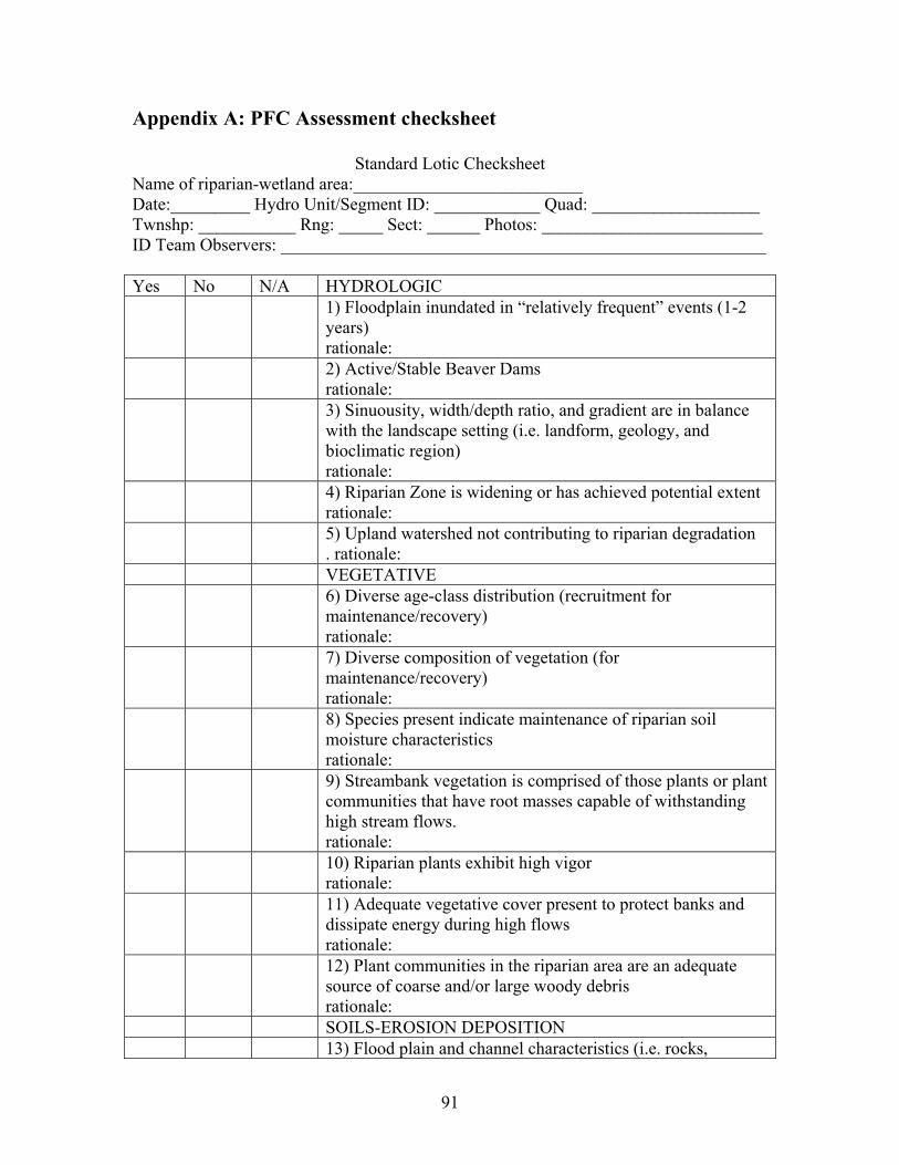
Appendix A: PFC Assessment checksheet

Standard Lotic Checksheet Name of riparian-wetland area:__________________________ Date:_________ Hydro Unit/Segment ID: ____________ Quad: ___________________ Twnshp: ___________ Rng: _____ Sect: ______ Photos: _________________________ ID Team Observers: _______________________________________________________ Yes No N/A HYDROLOGIC 1) Floodplain inundated in “relatively frequent” events (1-2

years) rationale:

2) Active/Stable Beaver Dams rationale:

3) Sinuousity, width/depth ratio, and gradient are in balance with the landscape setting (i.e. landform, geology, and bioclimatic region) rationale:

4) Riparian Zone is widening or has achieved potential extent rationale:

5) Upland watershed not contributing to riparian degradation . rationale:

VEGETATIVE 6) Diverse age-class distribution (recruitment for

maintenance/recovery) rationale:

7) Diverse composition of vegetation (for maintenance/recovery) rationale:

8) Species present indicate maintenance of riparian soil moisture characteristics rationale:

9) Streambank vegetation is comprised of those plants or plant communities that have root masses capable of withstanding high stream flows. rationale:

10) Riparian plants exhibit high vigor rationale:

11) Adequate vegetative cover present to protect banks and dissipate energy during high flows rationale:

12) Plant communities in the riparian area are an adequate source of coarse and/or large woody debris rationale:

SOILS-EROSION DEPOSITION 13) Flood plain and channel characteristics (i.e. rocks,

91

overflow channels, coarse and/or large woody debris) is adequate to dissipate energy rationale:

14) Point bars are revegetating rationale:

15) Lateral stream movement is associated with natural sinuosity rationale:

16) System is vertically stable rationale:

17) Stream is in balance with the water and sediment being supplied by the watershed (i.e. no excessive erosion or deposition) rationale:

Summary Determination Function Rating Proper Functioning Condition ___ Functional At-risk ___ Nonfunctional ___ Unknown ___ Trend for functional at-risk: Upward ___ Downward ___ Not Apparent ___ Rationale for rating: Are factors contributing to unacceptable conditions outside BLM’s control or management?

92

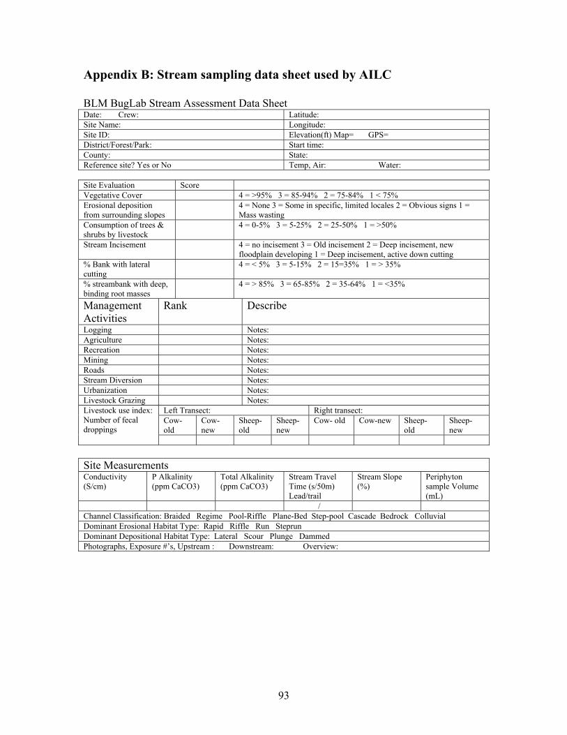
Appendix B: Stream sampling data sheet used by AILC

BLM BugLab Stream Assessment Data Sheet Date: Crew: Latitude: Site Name: Longitude: Site ID: Elevation(ft) Map= GPS= District/Forest/Park: Start time: County: State: Reference site? Yes or No Temp, Air: Water: Site Evaluation Score Vegetative Cover 4 = >95% 3 = 85-94% 2 = 75-84% 1 < 75% Erosional deposition from surrounding slopes

4 = None 3 = Some in specific, limited locales 2 = Obvious signs 1 = Mass wasting

Consumption of trees & shrubs by livestock

4 = 0-5% 3 = 5-25% 2 = 25-50% 1 = >50%

Stream Incisement 4 = no incisement 3 = Old incisement 2 = Deep incisement, new floodplain developing 1 = Deep incisement, active down cutting

% Bank with lateral cutting

4 = < 5% 3 = 5-15% 2 = 15=35% 1 = > 35%

% streambank with deep, binding root masses

4 = > 85% 3 = 65-85% 2 = 35-64% 1 = <35%

Management Activities

Rank Describe

Logging Notes: Agriculture Notes: Recreation Notes: Mining Notes: Roads Notes: Stream Diversion Notes: Urbanization Notes: Livestock Grazing Notes:

Left Transect: Right transect: Cow-old

Cow-new

Sheep- old

Sheep- new

Cow- old Cow-new Sheep- old

Sheep- new

Livestock use index: Number of fecal droppings

Site Measurements Conductivity (S/cm)

P Alkalinity (ppm CaCO3)

Total Alkalinity (ppm CaCO3)

Stream Travel Time (s/50m) Lead/trail

Stream Slope (%)

Periphyton sample Volume (mL)

/ Channel Classification: Braided Regime Pool-Riffle Plane-Bed Step-pool Cascade Bedrock Colluvial Dominant Erosional Habitat Type: Rapid Riffle Run Steprun Dominant Depositional Habitat Type: Lateral Scour Plunge Dammed Photographs, Exposure #’s, Upstream : Downstream: Overview:

93

94

Mean Depth (cm): Mean width (m): Transect 1 2 3 4 5 6 7 8 9 10 Width (m)

Depth (cm) at 0.25 width

Depth (cm) at 0.5 width

Depth (cm) at 0.75 width

Mean = Densiometer Measurements

(number of points shaded of 96) General Site Comments

Direction Unit 1

Unit 2 Unit 3 Unit 4 Upstream Left bank Right bank downstream

Stream Bed Particle Size Counts Unit 1 Unit 2 Unit 3 Unit 4

Particle size class (mm)

Totals Tallies Count Tallies Count Tallies Count Tallies Count

Bedrock 180 128 90 64 45 32 22.6 16 11 8 <8 Total # of particles counted: Median: