Journal of Hydrology 510 (2014) 164–181

Contents lists available at ScienceDirect

Journal of Hydrology

journal homepage: www.elsevier .com/locate / jhydrol

Evaluation of bed load transport formulae in a large regulated gravel bedriver: The lower Ebro (NE Iberian Peninsula)

0022-1694/$ - see front matter � 2013 Elsevier B.V. All rights reserved.http://dx.doi.org/10.1016/j.jhydrol.2013.12.014

⇑ Corresponding author. Tel.: +34 973 70 28 20.E-mail addresses: rlopez@eagrof.udl.cat (R. López), dvericat@macs.udl.cat

(D. Vericat), rbatalla@macs.udl.cat (R.J. Batalla).

Raúl López a,⇑, Damià Vericat b,c,d, Ramon J. Batalla b,c,e

a Department of Agricultural and Forest Engineering, University of Lleida, Av. Alcalde Rovira Roure, 191, E-25198 Lleida, Catalonia, Spainb Department of Environment and Soil Sciences, University of Lleida, Av. Alcalde Rovira Roure, 191, E-25198 Lleida, Catalonia, Spainc Forest Science Center of Catalonia, E-25280 Solsona, Catalonia, Spaind Institute of Geography and Earth Sciences, Aberystwyth University, Ceredigion SY23 3DB, Wales, UKe Catalan Institute for Water Research, H2O Building, E-17003 Girona, Catalonia, Spain

a r t i c l e i n f o

Article history:Received 5 June 2013Received in revised form 1 October 2013Accepted 7 December 2013Available online 16 December 2013This manuscript was handled byKonstantine P. Georgakakos, Editor-in-Chief,with the assistance of Ehab A. Meselhe,Associate Editor

Keywords:Bed load formulaeBed load transportGravel bed-riverArmored bed riverRiver Ebro

s u m m a r y

This paper tests the predictive power of 10 bed load formulae against bed load rates obtained for a largeregulated river (River Ebro) the armor layer of which is subject to repeated cycles of break-up and rees-tablishment. The theoretical principles of two of the 10 formulae explicitly include the effects of river bedarmoring. The results obtained showed substantial differences in equation performance but no evidentrelationship between predictive power and theoretical approach (e.g., discharge, stream power and prob-ability) was found. Overall, the predictive power of the tested formulae was relatively low. The averagepercentages of predicted bed load discharge that did not exceed factors of 2 (0.5 < r < 2) and 10(0.1 < r < 10) in relation to the observed discharge were 19% and 57%, respectively (where r is the discrep-ancy ratio between the predicted and observed values). In particular, the formulae of Yang (1984) andParker et al. (1982) presented the better levels of agreement with the observed bed load discharges.The bed load rating curve for the lower Ebro showed a similar degree of agreement to the best-perform-ing formulae. However, its predictive power was limited because only flow discharge acts as an indepen-dent variable and river bed dynamics, such as armoring cycles, are not contemplated.

� 2013 Elsevier B.V. All rights reserved.

1. Introduction

Bed load is the part of the bed material that moves episodicallyduring floods, either in traction (in rolling or sliding motion), or insaltation in the river channel. It controls the three-dimensionalmorphology of rivers and, in consequence, many fluvial researchand management applications require estimates of bed load. Bedload transport is a highly variable phenomenon, both in spaceand time. This variability is reflected in the functional relationsthat link flow intensity to bed load. Such relations have an uncer-tainty that can be placed at some orders of magnitude (Gomez andChurch, 1989). The origin of this lies partly in the highly local andunsteady nature of the driving forces but is also linked to changingrates of upstream sediment supply and to the composition andstructure of the river bed (Wilcock, 2001; Di Cristo et al., 2006;Greco et al., 2012).

The main reason for development of bed load equations is theneed to predict and plan in fluvial environments, and not only

for engineering purposes. Unfortunately, the collection of high-quality bed load transport data is an expensive and time-consum-ing task, and for many practical purposes recourse is made to a bedload transport formula (Gomez, 2006). Within this context, numer-ous bed load transport formulae have been developed over a cen-tury with the main purpose of predicting bed load, overcoming theinherent variability of sediment transport together with the uncer-tainties and difficulties associated with sampling. Formulae cover awide range of sediment sizes and hydraulic conditions. These for-mulae are based on the premise that specific relations exist be-tween hydraulic variables, sedimentary conditions, and rates ofbed load transport (Gomez and Church, 1989). Most of these mod-els have been derived from flume experimental data (e.g., fromearly studies such as Gilbert, 1914; Kramer, 1934; Casey, 1935;USWES, 1935; Shields, 1936; Chang, 1939; and lately Hamamori,1962) under steady and uniform flow conditions, rather than fromobservations of natural flow and transport. Few formulae derivefrom field measurements (e.g., Schoklitsch, 1950; Rottner, 1959;Parker et al., 1982; Bathurst, 2007). Inherent bed load transportvariability, the changing sedimentary conditions of the river bedand sampling efficiency are all key components that affect theperformance of equations. Equations are usually calibrated to

Notation

a dimensionless coefficientAgr threshold of mobilityC coefficientCs total bed-material concentration, ppm by weightDi particle size of percentile i, mDir reference value of Di, mDis particle size of percentile i of subsurface material, mDgr non-dimensional sediment size, mDm arithmetic mean diameter of sediment, mF1 adimensional parameter of fall velocityFgr sediment mobilization parameterg gravitational acceleration, m s�2

gr modified geometric mean value of rgwr weighted variation of grGgr dimensionless transport ratek Manning coefficient of roughness associated with skin

friction only, s m�1/3

k0 Manning coefficient of total roughness, s m�1/3

m exponentmr mean of discrepancy ratio (r)mlr mean of logarithm of discrepancy ratio (r)mqsp minimum value of qsp

n transition parameterN number of dataQ water discharge, m3 s�1

qc critical water discharge per unit width, m3 s�1 m�1

qc2 critical water discharge per unit width for transport asthe armor layer breaks up, m3 s�1 m�1

qs bed load discharge in weight per unit width, N s�1 m�1

qsm bed load discharge in mass per unit width, kg s�1 m�1

qso observed bed load discharge per unit width, N s�1 m�1

qsp predicted bed load discharge per unit width, N s�1 m�1

qsr reference value of qsm, kg s�1 m�1

qstv total bed-material load discharge in volume per unitwidth, m3 s�1 m�1

qstw total bed-material load discharge in weight per unitwidth, kp s�1 m�1

qsv bed load discharge in volume per unit width,m3 s�1 m�1

q� dimensionless volumetric bed load transport rate perunit width

r discrepancy ratio (qsp/qso)rw weighted value of rR hydraulic radius, mS bed or channel slope, m m�1

U� shear velocity, m s�1

V mean flow velocity, m s�1

Vc critical mean velocity, m s�1

ws fall velocity of sediment, m s�1

W� dimensionless bed loady mean flow depth, myr reference value of y, m/i excess Shields stressc specific weight of water, N m�3

cs specific weight of sediment, N m�3

m kinematic viscosity of water, m2 s�1

q density of water, kg m�3

qs density of sediment, kg m�3

s mean shear stress, N m�2

s� Shields numbers�i Shields stress for Dis

s�ri reference value of s�ix stream power per unit bed area, kg s�1 m�1

x0 stream power per unit weight of fluid, m s�1

xc critical unit stream power, kg s�1 m�1

(x �xc)r reference value of excess stream power, kg s�1 m�1

R. López et al. / Journal of Hydrology 510 (2014) 164–181 165

specific conditions used to derive them; these may be equilibriumconditions in the case of flume studies, but this is less likely forequations based on field data.

Since the initial comparison made by Johnson (1939) there havebeen several assessments of the performance of bed load transportformulae using both field and laboratory data (e.g., Shulits and Hill,1968; White et al., 1973; Carson and Griffith, 1987; Yang and Wan,1991; Chang, 1994; Reid et al., 1996; Batalla, 1997; Martin, 2003;Martin and Ham, 2005). Gomez and Church (1989) undertook oneof the most complete evaluations of bed load formulae and notedthat there are more bed load formulae than reliable data to testthem (Martin, 2003). These authors concluded that no formula per-forms consistently well; this can be attributed to the limitations ofthe test data and to the constraints of the test and the physics ofthe transport phenomenon. The results of analyses of the perfor-mance of these equations have been published elsewhere. Forexample, even in the best performing equations evaluated byWhite et al. (1975) fewer than 70% of the predicted sediment trans-port rates lay between half and twice the observed values. An-drews (1981) showed that the best equations for predicting bed-material discharges, within a range of half to twice the observedvalues, lay between 60% and 79% of the observations. Later, Batalla(1997) corroborated that the degree of accuracy between observedand predicted values varies greatly between one formula and an-other. He reported that the percentage of observations in whichthe discrepancy ratio between observed and computed valueshad a value of between 0.5 and 2 ranged from 25% (van Rijn) to38% (Brownlie), 52% (Meyer-Peter and Müller), 65% (Engelund

and Hansen), and 68% (Ackers and White). Most evaluations con-clude with a recommendation or representative formula, but nouniversal relationship between bed load discharge and hydraulicconditions has yet been established (Habersack and Laronne,2002). According to Wilcock (2001) the lack of field data to testbed load performance and to analyses bed load transport complex-ities (e.g., variability) are identified as the key reasons why we can-not expect to obtain high predictive power of equations underselected conditions. Testing and verifying formulae in large regu-lated rivers poses an additional challenge that has not been gener-ally treated in the literature. We specifically refer here to bedarmor condition and its periodic break-up and reformation; theseare not exclusive phenomena of rivers downstream from dams,since many natural gravel-bed rivers also show this behavior;but regulated rivers may exhibit more extreme conditions of sup-ply limitation and armor development. In addition, due to channeldimensions and flow magnitude, large rivers offer less opportunityto obtain direct field data; field information on such large systemsis, in general, sparse and scarce. Finally, regulated rivers are oftensubject to management actions, such as the release of periodicalflushing flows that may exacerbate channel adjustments (e.g.,Batalla and Vericat, 2009); those actions should preferably beplanned based on empirical data (in this case bed load and river-bed dynamics) that soundly informs modeling, design, and imple-mentation and re-evaluation avoiding, this way, completely blindengineering operations. Within this context, this paper principallyaims to assess the predictive power of a series of bed load formulaetested against bed load transport rates obtained for a large

166 R. López et al. / Journal of Hydrology 510 (2014) 164–181

regulated gravel bed river. Field data were obtained in the lowerRiver Ebro, downstream from the largest dam complex in the basin,for the period 2002–2004. This river undergoes cycles of break-upand reestablishment of its armor layer; this process has been con-templated in the analysis, but for a complete description, see Veri-cat and Batalla (2006) and Vericat et al. (2006a). Special attentionhas therefore been devoted to studying the performance of formu-lae under different armoring conditions; with the objective ofinforming users of these equations in rivers of similar characteris-tics where bed load data is unavailable. The novelty of this inves-tigation relies on the facts that we account for the texturalevolution of bed sediments during the study period, the choice ofinput grain size (surface vs. subsurface), and the armoring state.In particular, we show that undertaking analysis of equation per-formance as a function of the input grain-size is necessary as animportant factor controlling predicted results. We also presenthow the observed scatter in transport rates can be reduced byaccounting for textural evolution and armoring state, which sug-gests that these factors should be accounted for when predictingtransport rates.

2. Study reach and field measurements

2.1. The lower Ebro

The annual runoff of Ebro River basin is highly dependent ofmountain regions: the mountain area only represents about 30%of the total surface area of the Ebro basin but it is responsible fornearly 60% of its mean annual runoff (López and Justribó, 2010).The Ebro basin is extensively regulated by reservoirs: almost 190large dams regulate 67% (�7700 hm3) of the river’s mean annualrunoff. The largest reservoir complex is located in the lower courseof the river and was closed in 1969. It is comprised by three dams:Mequinenza, Ribarroja and Flix. Together, they impound 1750 hm3

of water (13% of the basin’s annual water yield). Frequent floods(i.e., Q2–Q25, where Qi is the discharge associated with an i-yearsrecurrence interval) have been reduced by 25% on average (Batallaet al., 2004), while large floods are no longer observed along thisreach.

Flow hydraulics and sediment transport were regularly andcontinuously monitored during floods at the Mora d’Ebre Monitor-ing Section (hereafter MEMS) during the period 2002–2004. Thissection of the river has a channel width of 160 m and is located27 km downstream from the Flix Dam. Along this reach, the riverflows as a single, low-sinuosity channel. The mean longitudinalchannel slope is 8.5 � 10�4. During the study, the median surfaceriver bed particle size D50 (where D is the size of the percentile iof the grain size distribution) in a gravel bar nearby MEMS rangedbetween 33 and 50 mm, while median subsurface size (D50s) ran-ged from 19 to 21 mm. According to these values the mean armor-ing ratio ranges between 1.6 and 2.6 (armor ratio is estimated asthe quotient between the surface and subsurface median particlesize, as per Parker et al., 1982).

The 2002–2003 and 2003–2004 study periods were averagehydrological years in terms of both the pre-dam and post-dam flowrecords (Vericat and Batalla, 2006). The mean discharge was415 m3 s�1 for the period 2002–2003 and 465 m3 s�1 for 2003–2004. Several floods (some of which were natural and some ofwhich were flushing flows for channel maintenance (see Batallaand Vericat, 2009)) occurred during the study period and almostall of them were monitored for sediment transport. The maximumrecorded discharge during the study period occurred in February2003 and reached 2500 m3/s (with return period of 8 years, esti-mated from the post-dam flow series at the downstream Tortosagauging station); so we consider this event to be a large flood in

the context of historic flood distribution i.e., largest recorded floodoccurred in 1907 and attained an estimated peak of 12,000 m3/s.The entire bed load is trapped in the upstream reservoir complex.As a result, the river does not receive any coarse-grained bed loadfractions from further upstream. However, the river partially main-tains its bed load transport capacity since floods still have enoughcompetence to entrain river bed sediments downstream from thedam (Vericat and Batalla, 2006).

2.2. Field measurements

Here we present a summary of the field methods used to mea-sure discharge, to characterize river bed sediments and to measurebed load at MEMS. Field measurements have already been exten-sively described by Vericat and Batalla (2006) and Vericat et al.(2006a, 2006b), and further referred in Batalla and Vericat (2009).

Flow was calculated at the monitoring section by routinghydrographs from an upstream gauging station operated by theEbro Water Authorities (Ascó, n. 163, 15 km upstream); and furthercompared with discharges in Tortosa (n. 27, 49 km downstream).Discharge measurements were used to corroborate flood hydro-graphs. Velocity of the flow was measured from the MEMS bridgeby means of an OTT C31 current meter which was attached to acable-suspended US DH74 sampler. Eleven velocity profiles wereobtained for instantaneous discharges between 750 and2160 m3 s�1. Mean velocities were calculated from velocity profilesand subsequently used to verify routed discharges from the up-stream gauging station.

For the purposes of this paper, we used the bed material grainsize distribution (i.e., surface and subsurface) that was obtainedfrom the closest exposed bar to MEMS. The bar is located less than500 m downstream (a distance equivalent to four times the meanchannel width). It is the nearest open and accessible gravel depositto the measuring site; we consider it fully representative of thegrain-size distribution of the active sediments in the river (formore details on Ebro’s grain size distribution see Vericat et al.,2006a). Additionally, inactive sediment, which was differentiatedby the vegetation cover, was avoided because it may have littlerelation with the current river regime. Bed material samplingwas performed on two occasions in relation to the river’s armoringcycle (see methods and results sections for a complete descriptionand discussion): (a) Bed Material I (hereafter BMI) was carried outin summer 2002, i.e., just before the beginning of the 2002–2003hydrological year; and (b) Bed Material II (hereafter BMII) wasundertaken in summer 2003, again just before the beginning ofthe 2003–2004 hydrological year. The coarse surface layer wascharacterized using the pebble count method (Wolman, 1954; Riceand Church, 1996) in the BMI characterization. A considerable pro-portion of fine material (i.e., particles finer than 8 mm) was foundat the bed surface in summer 2003 (i.e., BMII characterization); thesurface material was then sampled using the area-by-weightmethod (Kellerhals and Bray, 1971). This method offers the possi-bility of obtaining an accurate determination of the percentage offine material as this parameter is known to be underestimated bythe pebble count method. In both campaigns, the surface materialwas differentiated from the underlying sediment using spray paint(Lane and Carlson, 1953). The sampled area was then calculatedfollowing the Fripp and Diplas (1993) formula: A = 400(Dmax-s)2,where A is the area (m2) of the river bed surface that has to bepainted and sampled and Dmax-s is the b-axis (m) of the exposedparticle of maximum size. Area-by-weight samples were convertedto volumetric values (Kellerhals and Bray, 1971) applying a conver-sion factor of �0.5 (for more details, see Vericat et al. (2006a)). Thesubsurface material was sampled using the volumetric methodafter first removing the surface layer. The depth of the subsurfacelayer was around 0.3 m; this value lay within the range for the

R. López et al. / Journal of Hydrology 510 (2014) 164–181 167

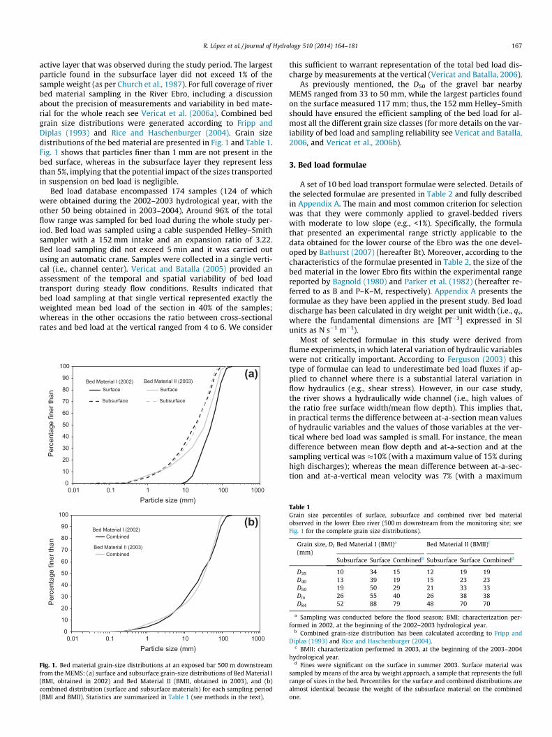
active layer that was observed during the study period. The largestparticle found in the subsurface layer did not exceed 1% of thesample weight (as per Church et al., 1987). For full coverage of riverbed material sampling in the River Ebro, including a discussionabout the precision of measurements and variability in bed mate-rial for the whole reach see Vericat et al. (2006a). Combined bedgrain size distributions were generated according to Fripp andDiplas (1993) and Rice and Haschenburger (2004). Grain sizedistributions of the bed material are presented in Fig. 1 and Table 1.Fig. 1 shows that particles finer than 1 mm are not present in thebed surface, whereas in the subsurface layer they represent lessthan 5%, implying that the potential impact of the sizes transportedin suspension on bed load is negligible.

Bed load database encompassed 174 samples (124 of whichwere obtained during the 2002–2003 hydrological year, with theother 50 being obtained in 2003–2004). Around 96% of the totalflow range was sampled for bed load during the whole study per-iod. Bed load was sampled using a cable suspended Helley–Smithsampler with a 152 mm intake and an expansion ratio of 3.22.Bed load sampling did not exceed 5 min and it was carried outusing an automatic crane. Samples were collected in a single verti-cal (i.e., channel center). Vericat and Batalla (2005) provided anassessment of the temporal and spatial variability of bed loadtransport during steady flow conditions. Results indicated thatbed load sampling at that single vertical represented exactly theweighted mean bed load of the section in 40% of the samples;whereas in the other occasions the ratio between cross-sectionalrates and bed load at the vertical ranged from 4 to 6. We consider

0

10

20

30

40

50

60

70

80

90

100

0.01 0.1 1 10 100 1000

Perc

enta

ge fi

ner t

han

Particle size (mm)

Surface Surface

Subsurface Subsurface

Bed Material II (2003)Bed Material I (2002)

0

10

20

30

40

50

60

70

80

90

100

0.01 0.1 1 10 100 1000

Perc

enta

ge fi

ner t

han

Particle size (mm)

Combined

CombinedBed Material II (2003)

Bed Material I (2002)(b)

(a)

Fig. 1. Bed material grain-size distributions at an exposed bar 500 m downstreamfrom the MEMS: (a) surface and subsurface grain-size distributions of Bed Material I(BMI, obtained in 2002) and Bed Material II (BMII, obtained in 2003), and (b)combined distribution (surface and subsurface materials) for each sampling period(BMI and BMII). Statistics are summarized in Table 1 (see methods in the text).

this sufficient to warrant representation of the total bed load dis-charge by measurements at the vertical (Vericat and Batalla, 2006).

As previously mentioned, the D50 of the gravel bar nearbyMEMS ranged from 33 to 50 mm, while the largest particles foundon the surface measured 117 mm; thus, the 152 mm Helley–Smithshould have ensured the efficient sampling of the bed load for al-most all the different grain size classes (for more details on the var-iability of bed load and sampling reliability see Vericat and Batalla,2006, and Vericat et al., 2006b).

3. Bed load formulae

A set of 10 bed load transport formulae were selected. Details ofthe selected formulae are presented in Table 2 and fully describedin Appendix A. The main and most common criterion for selectionwas that they were commonly applied to gravel-bedded riverswith moderate to low slope (e.g., <1%). Specifically, the formulathat presented an experimental range strictly applicable to thedata obtained for the lower course of the Ebro was the one devel-oped by Bathurst (2007) (hereafter Bt). Moreover, according to thecharacteristics of the formulae presented in Table 2, the size of thebed material in the lower Ebro fits within the experimental rangereported by Bagnold (1980) and Parker et al. (1982) (hereafter re-ferred to as B and P–K–M, respectively). Appendix A presents theformulae as they have been applied in the present study. Bed loaddischarge has been calculated in dry weight per unit width (i.e., qs,where the fundamental dimensions are [MT�3] expressed in SIunits as N s�1 m�1).

Most of selected formulae in this study were derived fromflume experiments, in which lateral variation of hydraulic variableswere not critically important. According to Ferguson (2003) thistype of formulae can lead to underestimate bed load fluxes if ap-plied to channel where there is a substantial lateral variation inflow hydraulics (e.g., shear stress). However, in our case study,the river shows a hydraulically wide channel (i.e., high values ofthe ratio free surface width/mean flow depth). This implies that,in practical terms the difference between at-a-section mean valuesof hydraulic variables and the values of those variables at the ver-tical where bed load was sampled is small. For instance, the meandifference between mean flow depth and at-a-section and at thesampling vertical was �10% (with a maximum value of 15% duringhigh discharges); whereas the mean difference between at-a-sec-tion and at-a-vertical mean velocity was 7% (with a maximum

Table 1Grain size percentiles of surface, subsurface and combined river bed materialobserved in the lower Ebro river (500 m downstream from the monitoring site; seeFig. 1 for the complete grain size distributions).

Grain size, Di

(mm)Bed Material I (BMI)a Bed Material II (BMII)c

Subsurface Surface Combinedb Subsurface Surface Combinedd

D35 10 34 15 12 19 19D40 13 39 19 15 23 23D50 19 50 29 21 33 33Dm 26 55 40 26 38 38D84 52 88 79 48 70 70

a Sampling was conducted before the flood season; BMI: characterization per-formed in 2002, at the beginning of the 2002–2003 hydrological year.

b Combined grain-size distribution has been calculated according to Fripp andDiplas (1993) and Rice and Haschenburger (2004).

c BMII: characterization performed in 2003, at the beginning of the 2003–2004hydrological year.

d Fines were significant on the surface in summer 2003. Surface material wassampled by means of the area by weight approach, a sample that represents the fullrange of sizes in the bed. Percentiles for the surface and combined distributions arealmost identical because the weight of the subsurface material on the combinedone.

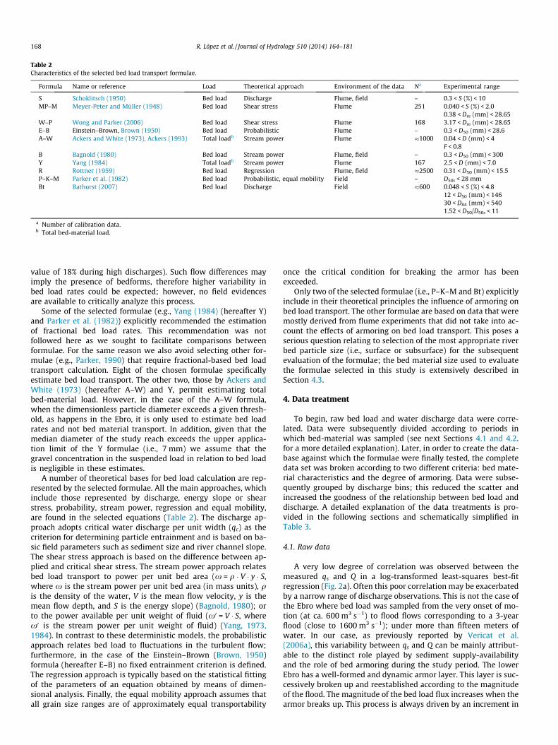
Table 2Characteristics of the selected bed load transport formulae.

Formula Name or reference Load Theoretical approach Environment of the data Na Experimental range

S Schoklitsch (1950) Bed load Discharge Flume, field – 0.3 < S (%) < 10MP–M Meyer-Peter and Müller (1948) Bed load Shear stress Flume 251 0.040 < S (%) < 2.0

0.38 < Dm (mm) < 28.65W–P Wong and Parker (2006) Bed load Shear stress Flume 168 3.17 < Dm (mm) < 28.65E–B Einstein–Brown, Brown (1950) Bed load Probabilistic Flume – 0.3 < D50 (mm) < 28.6A–W Ackers and White (1973), Ackers (1993) Total loadb Stream power Flume �1000 0.04 < D (mm) < 4

F < 0.8B Bagnold (1980) Bed load Stream power Flume, field – 0.3 < D50 (mm) < 300Y Yang (1984) Total loadb Stream power Flume 167 2.5 < D (mm) < 7.0R Rottner (1959) Bed load Regression Flume, field �2500 0.31 < D50 (mm) < 15.5P–K–M Parker et al. (1982) Bed load Probabilistic, equal mobility Field – D50s < 28 mmBt Bathurst (2007) Bed load Discharge Field �600 0.048 < S (%) < 4.8

12 < D50 (mm) < 14630 < D84 (mm) < 5401.52 < D50/D50s < 11

a Number of calibration data.b Total bed-material load.

168 R. López et al. / Journal of Hydrology 510 (2014) 164–181

value of 18% during high discharges). Such flow differences mayimply the presence of bedforms, therefore higher variability inbed load rates could be expected; however, no field evidencesare available to critically analyze this process.

Some of the selected formulae (e.g., Yang (1984) (hereafter Y)and Parker et al. (1982)) explicitly recommended the estimationof fractional bed load rates. This recommendation was notfollowed here as we sought to facilitate comparisons betweenformulae. For the same reason we also avoid selecting other for-mulae (e.g., Parker, 1990) that require fractional-based bed loadtransport calculation. Eight of the chosen formulae specificallyestimate bed load transport. The other two, those by Ackers andWhite (1973) (hereafter A–W) and Y, permit estimating totalbed-material load. However, in the case of the A–W formula,when the dimensionless particle diameter exceeds a given thresh-old, as happens in the Ebro, it is only used to estimate bed loadrates and not bed material transport. In addition, given that themedian diameter of the study reach exceeds the upper applica-tion limit of the Y formulae (i.e., 7 mm) we assume that thegravel concentration in the suspended load in relation to bed loadis negligible in these estimates.

A number of theoretical bases for bed load calculation are rep-resented by the selected formulae. All the main approaches, whichinclude those represented by discharge, energy slope or shearstress, probability, stream power, regression and equal mobility,are found in the selected equations (Table 2). The discharge ap-proach adopts critical water discharge per unit width (qc) as thecriterion for determining particle entrainment and is based on ba-sic field parameters such as sediment size and river channel slope.The shear stress approach is based on the difference between ap-plied and critical shear stress. The stream power approach relatesbed load transport to power per unit bed area (x = q � V � y � S,where x is the stream power per unit bed area (in mass units), qis the density of the water, V is the mean flow velocity, y is themean flow depth, and S is the energy slope) (Bagnold, 1980); orto the power available per unit weight of fluid (x0 = V � S, wherex0 is the stream power per unit weight of fluid) (Yang, 1973,1984). In contrast to these deterministic models, the probabilisticapproach relates bed load to fluctuations in the turbulent flow;furthermore, in the case of the Einstein–Brown (Brown, 1950)formula (hereafter E–B) no fixed entrainment criterion is defined.The regression approach is typically based on the statistical fittingof the parameters of an equation obtained by means of dimen-sional analysis. Finally, the equal mobility approach assumes thatall grain size ranges are of approximately equal transportability

once the critical condition for breaking the armor has beenexceeded.

Only two of the selected formulae (i.e., P–K–M and Bt) explicitlyinclude in their theoretical principles the influence of armoring onbed load transport. The other formulae are based on data that weremostly derived from flume experiments that did not take into ac-count the effects of armoring on bed load transport. This poses aserious question relating to selection of the most appropriate riverbed particle size (i.e., surface or subsurface) for the subsequentevaluation of the formulae; the bed material size used to evaluatethe formulae selected in this study is extensively described inSection 4.3.

4. Data treatment

To begin, raw bed load and water discharge data were corre-lated. Data were subsequently divided according to periods inwhich bed-material was sampled (see next Sections 4.1 and 4.2.for a more detailed explanation). Later, in order to create the data-base against which the formulae were finally tested, the completedata set was broken according to two different criteria: bed mate-rial characteristics and the degree of armoring. Data were subse-quently grouped by discharge bins; this reduced the scatter andincreased the goodness of the relationship between bed load anddischarge. A detailed explanation of the data treatments is pro-vided in the following sections and schematically simplified inTable 3.

4.1. Raw data

A very low degree of correlation was observed between themeasured qs and Q in a log-transformed least-squares best-fitregression (Fig. 2a). Often this poor correlation may be exacerbatedby a narrow range of discharge observations. This is not the case ofthe Ebro where bed load was sampled from the very onset of mo-tion (at ca. 600 m3 s�1) to flood flows corresponding to a 3-yearflood (close to 1600 m3 s�1); under more than fifteen meters ofwater. In our case, as previously reported by Vericat et al.(2006a), this variability between qs and Q can be mainly attribut-able to the distinct role played by sediment supply-availabilityand the role of bed armoring during the study period. The lowerEbro has a well-formed and dynamic armor layer. This layer is suc-cessively broken up and reestablished according to the magnitudeof the flood. The magnitude of the bed load flux increases when thearmor breaks up. This process is always driven by an increment in

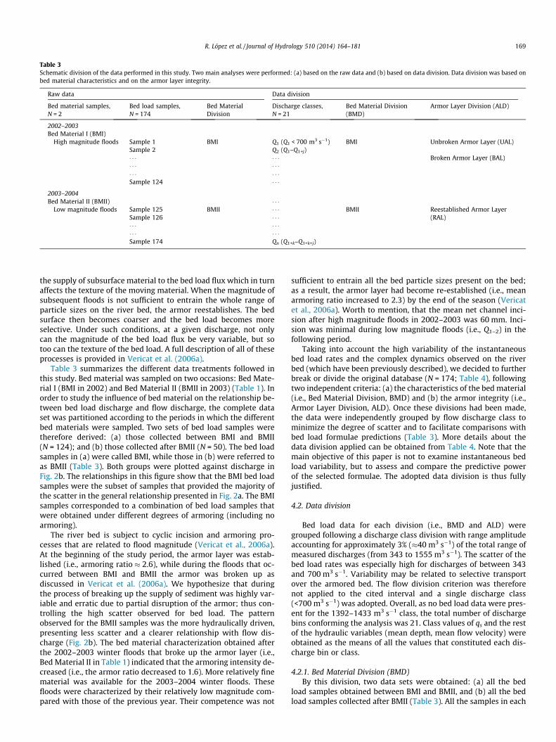
Table 3Schematic division of the data performed in this study. Two main analyses were performed: (a) based on the raw data and (b) based on data division. Data division was based onbed material characteristics and on the armor layer integrity.

Raw data Data division

Bed material samples,N = 2

Bed load samples,N = 174

Bed MaterialDivision

Discharge classes,N = 21

Bed Material Division(BMD)

Armor Layer Division (ALD)

2002–2003Bed Material I (BMI)

High magnitude floods Sample 1 BMI Q1 (Q1 < 700 m3 s�1) BMI Unbroken Armor Layer (UAL)Sample 2 Q2 (Q1–Q1+j)� � � � � � Broken Armor Layer (BAL)� � � � � �� � � � � �Sample 124 � � �

2003–2004Bed Material II (BMII) � � �

Low magnitude floods Sample 125 BMII � � � BMII Reestablished Armor Layer(RAL)Sample 126 � � �

� � � � � �� � � � � �Sample 174 Qn (Q1+k–Q1+k+j)

R. López et al. / Journal of Hydrology 510 (2014) 164–181 169

the supply of subsurface material to the bed load flux which in turnaffects the texture of the moving material. When the magnitude ofsubsequent floods is not sufficient to entrain the whole range ofparticle sizes on the river bed, the armor reestablishes. The bedsurface then becomes coarser and the bed load becomes moreselective. Under such conditions, at a given discharge, not onlycan the magnitude of the bed load flux be very variable, but sotoo can the texture of the bed load. A full description of all of theseprocesses is provided in Vericat et al. (2006a).

Table 3 summarizes the different data treatments followed inthis study. Bed material was sampled on two occasions: Bed Mate-rial I (BMI in 2002) and Bed Material II (BMII in 2003) (Table 1). Inorder to study the influence of bed material on the relationship be-tween bed load discharge and flow discharge, the complete dataset was partitioned according to the periods in which the differentbed materials were sampled. Two sets of bed load samples weretherefore derived: (a) those collected between BMI and BMII(N = 124); and (b) those collected after BMII (N = 50). The bed loadsamples in (a) were called BMI, while those in (b) were referred toas BMII (Table 3). Both groups were plotted against discharge inFig. 2b. The relationships in this figure show that the BMI bed loadsamples were the subset of samples that provided the majority ofthe scatter in the general relationship presented in Fig. 2a. The BMIsamples corresponded to a combination of bed load samples thatwere obtained under different degrees of armoring (including noarmoring).

The river bed is subject to cyclic incision and armoring pro-cesses that are related to flood magnitude (Vericat et al., 2006a).At the beginning of the study period, the armor layer was estab-lished (i.e., armoring ratio � 2.6), while during the floods that oc-curred between BMI and BMII the armor was broken up asdiscussed in Vericat et al. (2006a). We hypothesize that duringthe process of breaking up the supply of sediment was highly var-iable and erratic due to partial disruption of the armor; thus con-trolling the high scatter observed for bed load. The patternobserved for the BMII samples was the more hydraulically driven,presenting less scatter and a clearer relationship with flow dis-charge (Fig. 2b). The bed material characterization obtained afterthe 2002–2003 winter floods that broke up the armor layer (i.e.,Bed Material II in Table 1) indicated that the armoring intensity de-creased (i.e., the armor ratio decreased to 1.6). More relatively finematerial was available for the 2003–2004 winter floods. Thesefloods were characterized by their relatively low magnitude com-pared with those of the previous year. Their competence was not

sufficient to entrain all the bed particle sizes present on the bed;as a result, the armor layer had become re-established (i.e., meanarmoring ratio increased to 2.3) by the end of the season (Vericatet al., 2006a). Worth to mention, that the mean net channel inci-sion after high magnitude floods in 2002–2003 was 60 mm. Inci-sion was minimal during low magnitude floods (i.e., Q1–2) in thefollowing period.

Taking into account the high variability of the instantaneousbed load rates and the complex dynamics observed on the riverbed (which have been previously described), we decided to furtherbreak or divide the original database (N = 174; Table 4), followingtwo independent criteria: (a) the characteristics of the bed material(i.e., Bed Material Division, BMD) and (b) the armor integrity (i.e.,Armor Layer Division, ALD). Once these divisions had been made,the data were independently grouped by flow discharge class tominimize the degree of scatter and to facilitate comparisons withbed load formulae predictions (Table 3). More details about thedata division applied can be obtained from Table 4. Note that themain objective of this paper is not to examine instantaneous bedload variability, but to assess and compare the predictive powerof the selected formulae. The adopted data division is thus fullyjustified.

4.2. Data division

Bed load data for each division (i.e., BMD and ALD) weregrouped following a discharge class division with range amplitudeaccounting for approximately 3% (�40 m3 s�1) of the total range ofmeasured discharges (from 343 to 1555 m3 s�1). The scatter of thebed load rates was especially high for discharges of between 343and 700 m3 s�1. Variability may be related to selective transportover the armored bed. The flow division criterion was thereforenot applied to the cited interval and a single discharge class(<700 m3 s�1) was adopted. Overall, as no bed load data were pres-ent for the 1392–1433 m3 s�1 class, the total number of dischargebins conforming the analysis was 21. Class values of qs and the restof the hydraulic variables (mean depth, mean flow velocity) wereobtained as the means of all the values that constituted each dis-charge bin or class.

4.2.1. Bed Material Division (BMD)By this division, two data sets were obtained: (a) all the bed

load samples obtained between BMI and BMII, and (b) all the bedload samples collected after BMII (Table 3). All the samples in each

qs = 5·10 18 Q5.6; N = 174; R² = 0.27

0.0001

0.001

0.01

0.1

1

10

100

300 500 700 900 1100 1300 1500

q s(N

·s1 ·m

1 )

Q (m3·s 1)

qs = 5·10 22Q6.8; N = 124; R² = 0.29qs = 7·10 12Q3.7; N = 50; R² = 0.41

300 500 700 900 1100 1300 1500

Q (m3·s 1)

BM IBM II

(a) (b)

Fig. 2. Relation between observed unit bed load discharge and water discharge: (a) original database, and (b) original database divided by bed material: Bed Material I (BMI,bed load samples between summer 2002 and summer 2003) and Bed Material II (BMII, samples after summer 2003).

170 R. López et al. / Journal of Hydrology 510 (2014) 164–181

set were grouped in accordance with the discharge approach asoutlined above. The result of this treatment was a data set com-posed of 19 samples for the BMI condition and 17 samples for BMII(Table 4). As previously explained, the number of samples did notreach 21 because no bed load data were presented for one of thedischarge bins. This data set constitutes one of the two data group-ings against which the bed load formulae were tested in this paper.

Fig. 3a shows the relationship between qs and Q for subsets ofthe BMD. The degree of correlation of these relations was higherthan those obtained for the curves presented in Fig. 2b, the dataof which were not grouped by discharge class. However, inabsolute terms, the predictive power of the function still remainedlimited and well below previously adopted reference values fornon-linear i.e., power relationships (e.g., Barry et al., 2008).

4.2.2. Armor Layer Division (ALD)A preliminary analysis of the texture of the bed load samples

(Vericat et al., 2006a) and field observations showed that: (i) afterthe first flood in December 2002, the armor persisted; (ii) thefloods registered in February and March 2003 broke up the armorlayer; and (iii) the armor was reestablished during the November2003, December 2003 and May 2004 flood events. The bed loaddata set was then divided in line with these considerations (Ta-ble 3). A total of three armor layer conditions were identified: (a)Unbroken Armor Layer (hereafter UAL), (b) Broken Armor Layer(hereafter BAL), and (c) Reestablished Armor Layer (hereafterRAL). All of the samples in each division were grouped accordingto the discharge approach described above. The result of this treat-ment was a data set composed of 9 samples for the UAL condition,and 15 and 17 samples, respectively, for the BAL and RAL condi-tions (Table 4). As previously stated, the number of samples didnot reach 21 because no bed load data were presented for someoneof the discharge bins. It is necessary to consider that the RAL datasubset coincided with the BMII group in the Bed Material Division;this can be explained by the fact that all of the floods registeredafter the BMII bed characterization were classified as events inwhich the armor was reestablished. This data set constitutes thesecond of the two data groupings against which bed load formulaewere tested in this study.

Fig. 3b shows the relationship between qs and Q as a function ofthe armor integrity condition: UAL, BAL, and RAL. This figure showsbetter grouping and, certainly, correlations improved when thisdivision was considered; however, for UAL and BAL the regressioncoefficients (R2) are still poor. The BAL and UAL relations are at

opposite extremes and clearly represent different sediment supplyconditions. For a given discharge, a larger bed load discharge wouldbe expected for BAL than for UAL conditions. The RAL conditionrepresents an intermediate position, although it did not plot veryfar from the BAL relation (Fig. 3b).

4.3. Bed material input to formulae

Transport equations are sensitive to bed-material grain-size,which can differ by a factor of two or more between surface andsubsurface values in armored channels. Many older bed load equa-tions did not recognize different bed-material domains (i.e., sur-face, subsurface, combined) making unclear which grain-sizeshould be used to drive transport predictions. Worth to mentionthat laboratory mixtures used to derive bed load transport fromflume studies can be considered equivalent to the subsurface sed-iments typically found in the field, since they distinct input grain-size that are relevant for equation development and performance.Within this context, undertaking analysis of equation performanceas a function of the input grain-size is useful, if not necessary, tofurther highlight its importance as a controlling factor of predictedresults, as we do in this paper. The role of bed load texture (basedon bed load samples) improving formulae prediction was shownby Habersack and Laronne (2002) emphasizing the sensitivity ofmodel performance to bed material input. In our study, only 2 ofthe 10 tested formulae explicitly include in their theoretical prin-ciples the effects of river bed armoring: P–K–M and Bt (Table 2).For the remaining 8 formulae, different bed material feeding (or in-put) criteria were adopted in order to test the role of bed materialon bed load predictions. Specifically, the following considerationswere made when selecting the bed texture with which to run theanalysis:

1. Bed Material Division (BMI and BMII data sets): (A) a first run ofthe formulae was conducted using the subsurface grain size dis-tribution from the samples obtained in 2002 (i.e., BMI) and2003 (i.e., BMII, see Table 1 for more details). A total of 36 pre-dictions were obtained. (B) The formulae were subsequentlyrun using the surface grain size distributions obtained for eachperiod (i.e., BMI and BMII). As in the consideration (A), a total of36 predictions were calculated.

2. Armor Layer Division (UAL, BAL and RAL data sets): in this casethe texture inputs of the formulae were related to the armorcondition for each data set. (A) Unbroken Armor Layer (UAL):

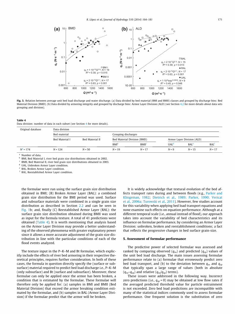
Table 4Data division: number of data in each subset (see Section 4 for more details).

Original database Data division

Bed material Grouping discharges

Bed Material I Bed Material II Bed Material Division (BMD) Armor Layer Division (ALD)

BMIb BMIIc UALd BALe RALf

Na = 174 N = 124 N = 50 N = 19 N = 17 N = 9 N = 15 N = 17

a Number of data.b BMI, Bed Material I, river bed grain size distributions obtained in 2002.c BMII, Bed Material II, river bed grain size distributions obtained in 2003.d UAL, Unbroken Armor Layer condition.e BAL, Broken Armor Layer condition.f RAL, Reestablished Armor Layer condition.

qs = 1·10-12Q3.9; N = 19R² = 0.30; p = 0.015

qs = 2·10-13Q4.1; N = 17R² = 0.63; p < 0.001

0.001

0.01

0.1

1

10

600 800 1000 1200 1400 1600

q s(N

·s1 ·m

1 )

Q (m3·s 1)

BM I

BM II

BMD

qs = 2·10-7Q2.3; N = 15R² = 0.39; p = 0.013

qs = 2·10-13Q4.1; N = 17R² = 0.63; p < 0.001

qs = 1·10-6exp0.008Q; N = 9R² = 0.45; p = 0.048

1E-05

0.0001

0.001

0.01

0.1

1

10

600 800 1000 1200 1400 1600

q s(N

·s1 ·m

1 )

Q (m3·s 1)

BAL

RAL

UAL

ALD(a) (b)

Fig. 3. Relation between average unit bed load discharge and water discharge. (a) Data divided by bed material (BMI and BMII) classes and grouped by discharge bins: BedMaterial Division (BMD). (b) Data divided by armoring integrity and grouped by discharge bins: Armor Layer Division (ALD) (see Section 4.2 for more details about data setsgrouping and division).

R. López et al. / Journal of Hydrology 510 (2014) 164–181 171

the formulae were run using the surface grain size distributionobtained in BMI; (B) Broken Armor Layer (BAL): a combinedgrain size distribution for the BMI period was used. Surfaceand subsurface materials were combined in a single grain sizedistribution as described in Section 2.2 and can be seen inFig. 1b; and, finally (C) Reestablished Armor Layer (RAL): thesurface grain size distribution obtained during BMII was usedas input for the formula texture. A total of 41 predictions wereobtained (Table 4). It is worth mentioning that analysis basedon the Armor Layer Division may provide a better understand-ing of the observed phenomena with greater explanatory powersince it allows a more accurate adjustment of the grain size dis-tribution in line with the particular conditions of each of theflood events analyzed.

The texture input in the P–K–M and Bt formulae, which explic-itly include the effects of river bed armoring in their respective the-oretical principles, requires further consideration. In both of thesecases, the formula in question directly specify the (surface or sub-surface) material required to predict bed load discharge i.e., P–K–M(only subsurface) and Bt (surface and subsurface). Moreover, theseformulae can only be applied once the armor has been broken, acondition that is estimated by the formulae. These formulae willtherefore only be applied for: (a) samples in BMI and BMII (BedMaterial Division) that exceed the armor breaking condition esti-mated by the formulae, and (b) samples in BAL (Armor Layer Divi-sion) if the formulae predict that the armor will be broken.

It is widely acknowledge that textural evolution of the bed af-fects transport rates during and between floods (e.g., Parker andKlingeman, 1982; Dietrich et al., 1989; Parker, 1990; Vericatet al., 2006a; Turowski et al., 2011). However, few studies accountfor this variability when applying bed load transport equations andnone examine such effects on equation performance. Although at adifferent temporal scale (i.e., annual instead of flood), our approachtakes into account the variability of bed characteristics and itsinfluence on formulae performance, by considering an Armor LayerDivision: unbroken, broken and reestablishment conditions; a factthat reflects the progressive changes in bed surface grain-size.

5. Assessment of formulae performance

The predictive power of selected formulae was assessed andranked by comparing observed (qso) and predicted (qsp) values ofthe unit bed load discharge. The main issues assessing formulaeperformance relate to (a) formulae that erroneously predict zerobed load transport, and (b) to the deviation between qso and qsp

that typically span a large range of values (both in absolute(qso–qsp) and relative (qso/qsp) terms).

These issues were addressed in the following way. Incorrectzero predictions (i.e., qsp = 0) may be obtained at low flow rates ifthe averaged predicted threshold value for particle entrainmentis not exceeded. Zero bed load predictions are incompatible withmany of the statistical indices commonly used to assess formulaeperformance. One frequent solution is the substitution of zero

172 R. López et al. / Journal of Hydrology 510 (2014) 164–181

predictions by a minimum value of bed load discharge (e.g., Barryet al., 2004, 2007; Recking, 2010). Occasionally, if the proportion ofzero predictions is significant, some indices may end up asfunctions of the minimum adopted values of qsp rather than as realindicators of formula performance (e.g., Barry et al., 2007). In thisstudy, we took a minimum value of qsp (mqsp) adapted to the min-imum observed value of qso for each of the data subgroups (BMDand ALD), but based on a sensitivity analysis undertaken for thedifferent statistical indices. We examined the effect of a widevariation of mqsp (i.e., between 1 � 10�9 and 1 � 10�2 N s�1 m�1)for all the statistical indices. Although these indices are properlyintroduced further in the text, this analysis illustrated as equationsshowed progressively better adjustment with the increase of themqsp value adopted for predictions 0. It is worth to mentions, theselected value of mqsp only begins to affect the arithmetic meanof the discrepancy ratio (i.e., mr, index further introduced) for al-most all the equations when mqsp was greater than a given value;a value that was adopted for selecting mqsp for each data division.Specifically, in the case of the Bed Material Division database thecritical value of mqsp was around 1 � 10�3N s�1 m�1, representingthe 65% of the minimum qso, which was exceeded by 93% of thevalues in the original dataset (N = 174). In the case of the ArmorLayer Division database, however, the critical value of mqsp wasaround 4 � 10�5N s�1 m�1, a value that represented 62% of theminimum qso, which was exceeded by 99% of the values in theoriginal dataset.

Several statistical indices and graphical methods were used toassess the performance of the different formulae. These indicesare based on the discrepancy ratio (r) between the predicted andobserved values (r = qsp/qso). The range of this ratio is (0, +1). Inbed load studies r can span a large range of values: frequentlytwo or more orders of magnitude (e.g., Duan et al., 2006; Recking,2010). Statistical comparisons should therefore also include logtransformations and indices that are less sensitive to extremevalues.

First, we calculated the percentage of qsp that did not exceed afactor of 2 (0.5 < r < 2), 5 (0.2 < r < 5) and 10 (0.1 < r < 10) in rela-tion to qso. The arithmetic mean of r (mr) was also used:

mr ¼ ð1=NÞXN

i¼1

ri ð1Þ

where ri is the i value of r, and N is the number of data. This value isin the range (0, +1), with values close to 1 indicating less discrep-ancy. The arithmetic mean of logr (mlr) was also used:

mlr ¼ ð1=NÞXN

i¼1

log ri ð2Þ

where ri is the ith value of r, and N is the number of data. This valueis in the range (�1, +1), with values close to 0 indicating less dis-crepancy. A modified type of geometric mean value of r (gr) (Haber-sack and Laronne, 2002) was also used:

gr ¼ ðr1r2 � � � ri � � � rNÞ1=N ð3Þ

where the reciprocal value is used if ri < 1, ensuring that gr P 1. Thisvalue is in the range (1, +1), with low values indicating the smallestdiscrepancies. A weighted variation of the gr index (gwr) (Habersackand Laronne, 2002) was also used:

gwr ¼ ðrw1rw2 � � � rwi � � � rwNÞ1=N ð4Þ

where rw is a value of r weighted by the power of the observed bedload discharge ðrw ¼ rqso Þ and where the reciprocal value is used ifrwi < 1, ensuring that gwr P 1. This value is in the range (1, +1),with low values indicating the smallest discrepancies between qsp

and qso.

We also graphically examined (at the log scale) the deviationbetween qso and qsp for each bed load transport value and we ana-lyzed the distribution of the discrepancy ratio (r) using a box-plotdiagram at the logarithmic scale. The ranking of the performancesof different formulae may vary according to the statistical proper-ties of the indices in question (e.g., Habersack and Laronne, 2002;Barry et al., 2007). For instance, the mr index is more sensitive tor values larger than 1 (i.e., a value of r = 10 weighs more in themr computation than a value of 0.1, despite the fact that both rep-resent a deviation of one order of magnitude with respect to thesymmetry axes r = 1). The mr index is therefore less sensitive tothe proportion of zero predictions and also to the minimumadopted value of qsp. In contrast, in the mrl index, errors of equalmagnitude weigh the same, independently of their relative posi-tions with respect to the symmetry axes log r = 0 (e.g., r = 10 andr = 0.1). It is therefore more sensitive to the proportion of zero pre-dictions and to the minimum adopted value of qsp. A limitation ofmlr is that logr values of the same magnitude and opposite signscancel each other out, yielding mlr = 0. This index is therefore moresensitive to small but asymmetrical deviations (e.g., if r1 = 1.5 andr2 = 2 then mlr = 0.24) than to larger symmetrical deviations (e.g., ifr1 = 0.01 and r2 = 100 then mlr = 0). Furthermore, gr is less sensitivethan mr to high values of r (i.e., r� 1) because it is based on thegeometric mean; however, it is more sensitive to zero predictions,since a reciprocal value is taken if r < 1. Finally, the gwr index ismore sensitive to deviations of large qso values. Previous works(e.g., Barry et al., 2007) conclude that, given the potential bias oferror index, there is no perfect method for assessing equation per-formance, especially in those cases that allows for inclusion ofincorrect zero predictions.

The performance of the formulae is ranked for each index. Theglobal performance of the formulae is assessed on the basis of acombination of three different criteria: (a) the relative positionfor each index, (b) the frequency with which the formulae arelocated in the top five positions, and (c) the ratio between theindex value obtained using a given formula and the lowest indexvalue (i.e., this last value is determined by the lowest rankedformula). We also present the log scale comparison betweenqsp and qso for the Bed Material and Armor Layer divisions.Finally, we present a box plot in log scale corresponding to thedistribution of the discrepancy ratio (r) for: (a) BMD (fed withsubsurface bed material), (b) BMD (fed with surface bed mate-rial), and (c) ALD divisions.

6. Bed load regime

A full description of the flow and bed load regime during theperiod 2002–2004 was reported by Vericat and Batalla (2006);hence, only a brief summary is presented here to contextualizethe main results of this paper. Bed load was sampled duringalmost all of the floods recorded during that period. The meanbed load rate was 1.36 N s�1 m�1 in 2002–2003 (i.e., BMI) and0.65 � 10�1 N s�1 m�1 in 2003–2004 (i.e., BMII). Worth to noticethat that bed load rates during the first period show a highly var-iable pattern for a given discharge (Fig. 2b), contributing to a highscatter in the plot. Maximum rates were recorded in 2002–2003,with an instantaneous maximum value of 11.8 N s�1 m�1 (forfurther details, see Vericat and Batalla (2006)).

Bed load texture was markedly different in the two periods. Themedian bed load particle size in the samples collected during theperiod 2002–2003 varied from 1 to 72 mm, while for 2003–2004this range decreased to 4–44 mm, showing a more selective trans-port range. The upper limits of both ranges corresponded to the D70

and D65 of the bed surface grain size distribution obtained in 2002and 2003 respectively (Fig. 1). The lower limit was not present in

R. López et al. / Journal of Hydrology 510 (2014) 164–181 173

the surface sediments sampled in 2002 and represents the D15 ofthe 2003 distribution.

The original database (N = 174) was grouped according to thepreviously reported discharge class division in order to define abed load rating curve for the lower Ebro. Note that in this case datawere not divided according to any specific bed material or armorintegrity criteria. The corresponding bed load transport model is:

qs ¼ 4� 10�10 Q 3:11 ð5Þ

(R2 = 0.46, N = 21, p = 7.3 � 10�4). The statistical indices applied forthe formulae were also obtained for Eq. (5). Note that this equationis not comparable with the rest of assessed formulae, since it is aregression equation derived from own data of the study reach.Although indices for Eq. (5) were not taken into account in the rank-ing of the formulae, they are shown at the bottom of Tables 5–7 inorder to facilitate comparisons between the Ebro bed load modeland the 10 different formulae that were selected.

7. Testing the formulae

7.1. Bed Material Division

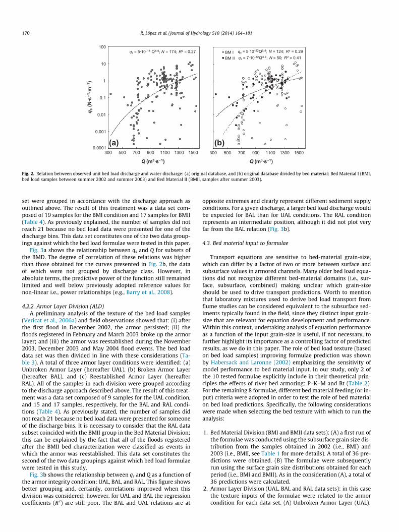
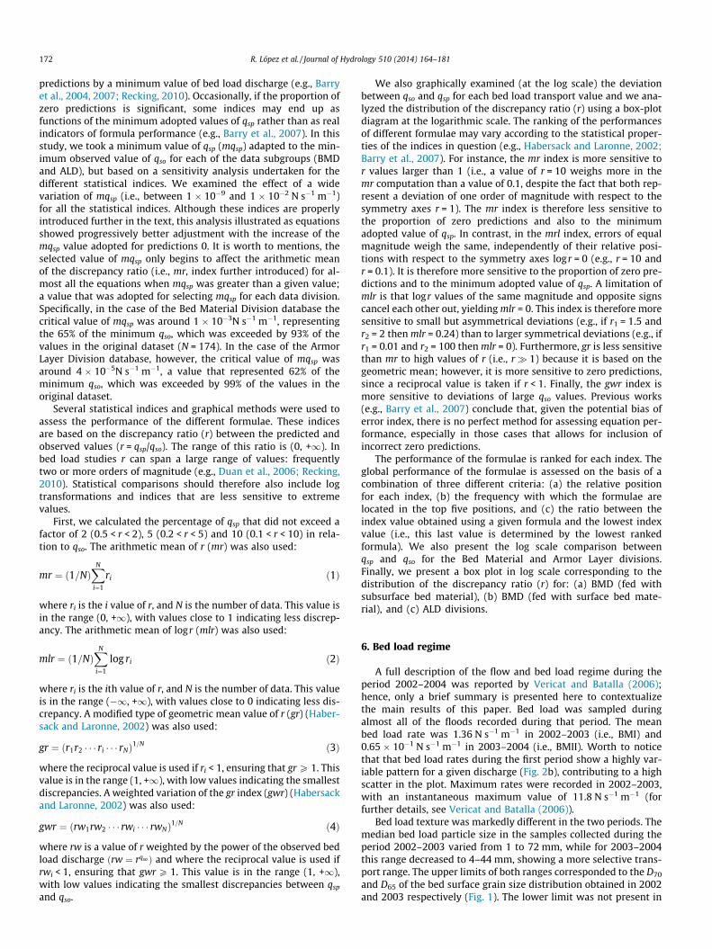
Tables 5 and 6 show the statistical indices according to the BedMaterial Division and considering the different sediment grain-sizescenarios (i.e., subsurface and surface, respectively). In these ta-bles, the value of each statistical index is ordered from the smallestto the largest discrepancy between the values for qsp and qso; this isa way of ranking the predictive power of each formula. It is impor-tant to note that we have included formulae that explicitly con-sider the presence of an armor layer (i.e., P–K–M and Bt) (Tables5 and 6) despite these formulae directly specify the material (i.e.,surface and/or subsurface) required to predict bed load discharge(see Section 4.3).

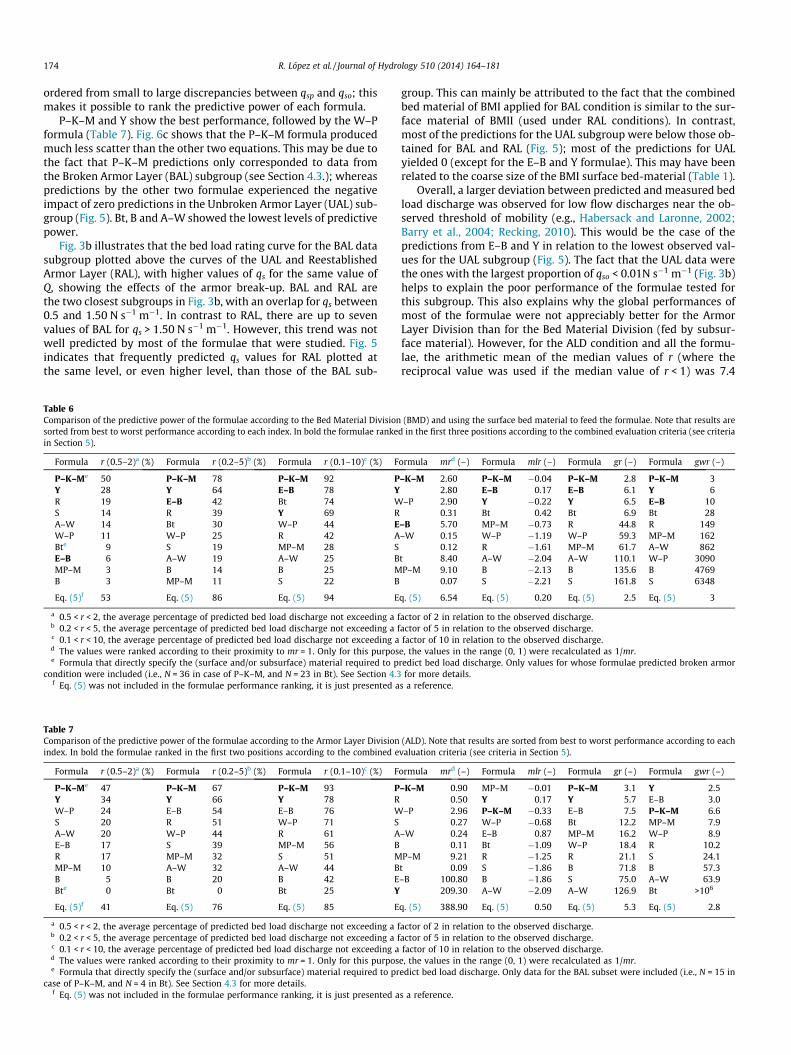
When we used subsurface grain size distribution in the BMDthe overall best fit was provided by P–K–M, B, Y and the Rottner(1959) (hereafter R) formulae (Table 5). This can be seen in Figs. 4and 6a in which these three formulae show less scatter than theothers. The worst performing formulae were those of Meyer-Peterand Müller (1948) (hereafter MP–M), E–B and Wong and Parker(2006) (hereafter W–P); mainly due to their trend to overpredict.When the surface bed material was used in the BMD, there weresmaller discrepancies between P–K–M and Y and the observed data

Table 5Comparison of the predictive power of the formulae according to the Bed Material Divisionare sorted from best to worst performance according to each index. In bold the formulaecriteria in Section 5).

Formula r (0.5–2)a (%) Formula r (0.2–5)b (%) Formula r (0.1–10)c (%) F

P–K–Me 50 B 83 B 97 AB 47 Y 83 P–K–M 92 PY 44 P–K–M 78 Y 89 BA–W 36 S 75 R 89 RR 28 R 67 S 86 YS 25 A–W 67 Bt 74 BBte 9 Bt 30 A–W 72 SW–P 0 W–P 14 W–P 28 WE–B 0 E–B 8 E–B 28 EMP–M 0 MP–M 3 MP–M 11 M

Eq. (5)f 53 Eq. (5) 86 Eq. (5) 94 E

a 0.5 < r < 2, the average percentage of predicted bed load discharge not exceeding a fb 0.2 < r < 5, the average percentage of predicted bed load discharge not exceeding a fc 0.1 < r < 10, the average percentage of predicted bed load discharge not exceeding ad The values were ranked according to their proximity to mr = 1. Only for this purpose Formula that directly specify the (surface and/or subsurface) material required to p

condition were included (i.e., N = 36 in case of P–K–M, and N = 23 in Bt). See Section 4.3f Eq. (5) was not included in the formulae performance ranking, it is just presented a

(Table 6). However, Fig. 6b reveals that Y produced greater scatterfor r than P–K–M (especially for the lower limit, since the Y for-mula predicted no bed load discharge (i.e., zero bed load) for 5 val-ues (see Fig. 4)). The E–B formula performed well, although itshowed a larger scatter of r between percentiles 25 and 75(Fig. 6b). The worst performing formulae were B and S, mainly be-cause they tended to underestimation (Figs. 4 and 6b).

Figs. 4, 6a and b illustrate an overall tendency to underestimate(e.g., median discrepancy ratio r < 1) when surface material isused; in contrast, overestimation occurs when subsurface materialis used as a grain-size predictive variable (e.g., median discrepancyratio r > 1). All the formulae (except P–K–M and Bt) that use sub-surface material yielded an arithmetic mean of the median valuesof r (where the reciprocal value was used if the median value ofr < 1) of 9.3, with a coefficient of variation of 125%. When surfacematerial was used, the arithmetic mean of the median values of r(where the reciprocal value was used if the median value ofr < 1) was 112 and the coefficient of variation was 126%. Underes-timation using surface material is therefore, on average, one orderof magnitude higher than overestimation using subsurface mate-rial. This pattern can mainly be attributed to the fact that surfacematerial was too coarse to be theoretically entrained for most ofthe eight formulae. In similar way, the relative fine texture of thesubsurface materials drives to overprediction. Fig. 4 illustratesthe different proportion of zero bed load predictions when usingsurface and subsurface materials.

Finally, armoring was greater for BMI than for BMII (Table 1).This may explain the larger discrepancy between the predictionswhen surface and subsurface materials were alternatively used tofeed the formulae under the BMI division (Fig. 4). In some casesthis discrepancy was notably large since the surface material forBMI was too coarse for the flow to exceed the predictedentrainment threshold (which was based on the formulation, seeAppendix A). This was evident, especially for equations S, B, W–Pand A–W; none of these equations showed more than three values(for BMI surface material) that exceeded the entrainment conditionvalue (Fig. 4).

7.2. Armor Layer Division

Table 7 shows the values of indices according to the ArmorLayer Division. In this table, each of the statistical index values is

(BMD) and using the subsurface bed material to feed the formulae. Note that resultsranked in the first four positions according to the combined evaluation criteria (see

ormula mrd (–) Formula mlr (–) Formula gr (–) Formula gwr (–)

–W 1.7 P–K–M �0.04 B 2.4 P–K–M 2.60–K–M 2.6 B �0.09 Y 2.7 R 2.75

2.9 R 0.21 P–K–M 2.8 S 2.774.0 Y 0.30 S 3.7 Y 2.797.1 A–W �0.34 R 3.8 A–W 3.70

t 8.4 Bt 0.42 A–W 5.0 B 4.6020.2 S 0.52 Bt 6.9 W–P 10.39

–P 98.7 W–P 1.27 W–P 18.7 E–B 12.59–B 152.5 E–B 1.34 E–B 21.7 Bt 28.16P–M 237.3 MP–M 1.62 MP–M 41.9 MP–M 29.06

q. (5) 6.5 Eq. (5) 0.20 Eq. (5) 2.5 Eq. (5) 2.95

actor of 2 in relation to the observed discharge.actor of 5 in relation to the observed discharge.factor of 10 in relation to the observed discharge.

e, the values in the range (0, 1) were recalculated as 1/mr.redict bed load discharge. Only values for whose formulae predicted broken armor

for more details.s a reference.

174 R. López et al. / Journal of Hydrology 510 (2014) 164–181

ordered from small to large discrepancies between qsp and qso; thismakes it possible to rank the predictive power of each formula.

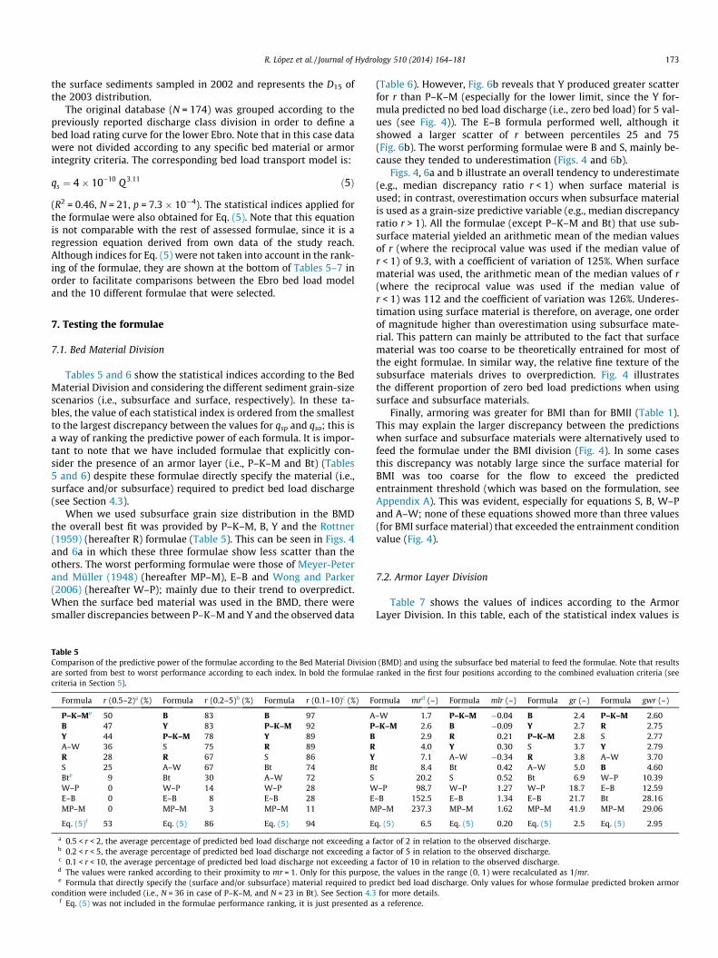
P–K–M and Y show the best performance, followed by the W–Pformula (Table 7). Fig. 6c shows that the P–K–M formula producedmuch less scatter than the other two equations. This may be due tothe fact that P–K–M predictions only corresponded to data fromthe Broken Armor Layer (BAL) subgroup (see Section 4.3.); whereaspredictions by the other two formulae experienced the negativeimpact of zero predictions in the Unbroken Armor Layer (UAL) sub-group (Fig. 5). Bt, B and A–W showed the lowest levels of predictivepower.

Fig. 3b illustrates that the bed load rating curve for the BAL datasubgroup plotted above the curves of the UAL and ReestablishedArmor Layer (RAL), with higher values of qs for the same value ofQ, showing the effects of the armor break-up. BAL and RAL arethe two closest subgroups in Fig. 3b, with an overlap for qs between0.5 and 1.50 N s�1 m�1. In contrast to RAL, there are up to sevenvalues of BAL for qs > 1.50 N s�1 m�1. However, this trend was notwell predicted by most of the formulae that were studied. Fig. 5indicates that frequently predicted qs values for RAL plotted atthe same level, or even higher level, than those of the BAL sub-

Table 6Comparison of the predictive power of the formulae according to the Bed Material Divisionsorted from best to worst performance according to each index. In bold the formulae rankein Section 5).

Formula r (0.5–2)a (%) Formula r (0.2–5)b (%) Formula r (0.1–10)c (%) F

P–K–Me 50 P–K–M 78 P–K–M 92 PY 28 Y 64 E–B 78 YR 19 E–B 42 Bt 74 WS 14 R 39 Y 69 RA–W 14 Bt 30 W–P 44 EW–P 11 W–P 25 R 42 ABte 9 S 19 MP–M 28 SE–B 6 A–W 19 A–W 25 BMP–M 3 B 14 B 25 MB 3 MP–M 11 S 22 B

Eq. (5)f 53 Eq. (5) 86 Eq. (5) 94 E

a 0.5 < r < 2, the average percentage of predicted bed load discharge not exceeding a fb 0.2 < r < 5, the average percentage of predicted bed load discharge not exceeding a fc 0.1 < r < 10, the average percentage of predicted bed load discharge not exceeding ad The values were ranked according to their proximity to mr = 1. Only for this purpose Formula that directly specify the (surface and/or subsurface) material required to p

condition were included (i.e., N = 36 in case of P–K–M, and N = 23 in Bt). See Section 4.3f Eq. (5) was not included in the formulae performance ranking, it is just presented a

Table 7Comparison of the predictive power of the formulae according to the Armor Layer Divisionindex. In bold the formulae ranked in the first two positions according to the combined e

Formula r (0.5–2)a (%) Formula r (0.2–5)b (%) Formula r (0.1–10)c (%) F

P–K–Me 47 P–K–M 67 P–K–M 93 PY 34 Y 66 Y 78 RW–P 24 E–B 54 E–B 76 WS 20 R 51 W–P 71 SA–W 20 W–P 44 R 61 AE–B 17 S 39 MP–M 56 BR 17 MP–M 32 S 51 MMP–M 10 A–W 32 A–W 44 BB 5 B 20 B 42 EBte 0 Bt 0 Bt 25 Y

Eq. (5)f 41 Eq. (5) 76 Eq. (5) 85 E

a 0.5 < r < 2, the average percentage of predicted bed load discharge not exceeding a fb 0.2 < r < 5, the average percentage of predicted bed load discharge not exceeding a fc 0.1 < r < 10, the average percentage of predicted bed load discharge not exceeding ad The values were ranked according to their proximity to mr = 1. Only for this purpose Formula that directly specify the (surface and/or subsurface) material required to pr

case of P–K–M, and N = 4 in Bt). See Section 4.3 for more details.f Eq. (5) was not included in the formulae performance ranking, it is just presented a

group. This can mainly be attributed to the fact that the combinedbed material of BMI applied for BAL condition is similar to the sur-face material of BMII (used under RAL conditions). In contrast,most of the predictions for the UAL subgroup were below those ob-tained for BAL and RAL (Fig. 5); most of the predictions for UALyielded 0 (except for the E–B and Y formulae). This may have beenrelated to the coarse size of the BMI surface bed-material (Table 1).

Overall, a larger deviation between predicted and measured bedload discharge was observed for low flow discharges near the ob-served threshold of mobility (e.g., Habersack and Laronne, 2002;Barry et al., 2004; Recking, 2010). This would be the case of thepredictions from E–B and Y in relation to the lowest observed val-ues for the UAL subgroup (Fig. 5). The fact that the UAL data werethe ones with the largest proportion of qso < 0.01N s�1 m�1 (Fig. 3b)helps to explain the poor performance of the formulae tested forthis subgroup. This also explains why the global performances ofmost of the formulae were not appreciably better for the ArmorLayer Division than for the Bed Material Division (fed by subsur-face material). However, for the ALD condition and all the formu-lae, the arithmetic mean of the median values of r (where thereciprocal value was used if the median value of r < 1) was 7.4

(BMD) and using the surface bed material to feed the formulae. Note that results ared in the first three positions according to the combined evaluation criteria (see criteria

ormula mrd (–) Formula mlr (–) Formula gr (–) Formula gwr (–)

–K–M 2.60 P–K–M �0.04 P–K–M 2.8 P–K–M 32.80 E–B 0.17 E–B 6.1 Y 6

–P 2.90 Y �0.22 Y 6.5 E–B 100.31 Bt 0.42 Bt 6.9 Bt 28

–B 5.70 MP–M �0.73 R 44.8 R 149–W 0.15 W–P �1.19 W–P 59.3 MP–M 162

0.12 R �1.61 MP–M 61.7 A–W 862t 8.40 A–W �2.04 A–W 110.1 W–P 3090P–M 9.10 B �2.13 B 135.6 B 4769

0.07 S �2.21 S 161.8 S 6348

q. (5) 6.54 Eq. (5) 0.20 Eq. (5) 2.5 Eq. (5) 3

actor of 2 in relation to the observed discharge.actor of 5 in relation to the observed discharge.factor of 10 in relation to the observed discharge.

e, the values in the range (0, 1) were recalculated as 1/mr.redict bed load discharge. Only values for whose formulae predicted broken armor

for more details.s a reference.

(ALD). Note that results are sorted from best to worst performance according to eachvaluation criteria (see criteria in Section 5).

ormula mrd (–) Formula mlr (–) Formula gr (–) Formula gwr (–)

–K–M 0.90 MP–M �0.01 P–K–M 3.1 Y 2.50.50 Y 0.17 Y 5.7 E–B 3.0

–P 2.96 P–K–M �0.33 E–B 7.5 P–K–M 6.60.27 W–P �0.68 Bt 12.2 MP–M 7.9

–W 0.24 E–B 0.87 MP–M 16.2 W–P 8.90.11 Bt �1.09 W–P 18.4 R 10.2

P–M 9.21 R �1.25 R 21.1 S 24.1t 0.09 S �1.86 B 71.8 B 57.3–B 100.80 B �1.86 S 75.0 A–W 63.9

209.30 A–W �2.09 A–W 126.9 Bt >106

q. (5) 388.90 Eq. (5) 0.50 Eq. (5) 5.3 Eq. (5) 2.8

actor of 2 in relation to the observed discharge.actor of 5 in relation to the observed discharge.factor of 10 in relation to the observed discharge.

e, the values in the range (0, 1) were recalculated as 1/mr.edict bed load discharge. Only data for the BAL subset were included (i.e., N = 15 in

s a reference.

0.001 0.01 0.1 1 10

BM IBM II

b) MP-M

0.001 0.01 0.1 1 10

BM IBM II

b) S

0.001

0.01

0.1

1

10

0.001 0.01 0.1 1 10

a) S

0.001

0.01

0.1

1

10

0.001 0.01 0.1 1 10

a) W-P

0.001 0.01 0.1 1 10

BM IBM II

b) W-P

0.001

0.01

0.1

1

10

0.001 0.01 0.1 1 10

a) E-B

0.001 0.01 0.1 1 10

BM IBM II

b) E-B

0.001

0.01

0.1

1

10

0.001 0.01 0.1 1 10

a) MP-M

0.001

0.01

0.1

1

10

0.001 0.01 0.1 1 10

a) A-W

0.001 0.01 0.1 1 10

BM IBM II

b) A-W

0.001

0.01

0.1

1

10

0.001 0.01 0.1 1 10

a) B

0.001

0.01

0.1

1

10

0.001 0.01 0.1 1 10

a) Y

0.001 0.01 0.1 1 10

BM IBM II

b) Y

0.001

0.01

0.1

1

10

0.001 0.01 0.1 1 10

a) R

0.001 0.01 0.1 1 10

qs observed (N·s 1·m 1)

BM IBM II

b) R

0.001 0.01 0.1 1 10

BM IBM II

Bt

0.001

0.01

0.1

1

10

0.001 0.01 0.1 1 10

q spr

edic

ted

(N·s

1 ·m

1 )

BM IBM II

P-K-M

0.001

0.01

0.1

1

10

0.001 0.01 0.1 1 10

BM IBM II

Eq. (5)

0.001 0.01 0.1 1 10

BM IBM II

b) B

qs observed (N·s 1·m 1)qs observed (N·s 1·m 1)qs observed (N·s 1·m 1)

q spr

edic

ted

(N·s

1 ·m

1 )q s

pred

icte

d (N

·s1 ·

m1 )

q spr

edic

ted

(N·s

1 ·m

1 )q s

pred

icte

d (N

·s1 ·

m1 ) ( (

((

(

( (

(

( (

((

( (

((

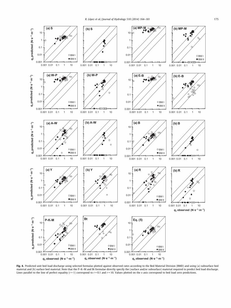
Fig. 4. Predicted unit bed load discharge using selected formulas plotted against observed rates according to the Bed Material Division (BMD) and using (a) subsurface bedmaterial and (b) surface bed material. Note that the P–K–M and Bt formulae directly specify the (surface and/or subsurface) material required to predict bed load discharge.Lines parallel to the line of perfect equality (r = 1) correspond to r = 0.1 and r = 10. Values plotted on the x axis correspond to bed load zero predictions.

R. López et al. / Journal of Hydrology 510 (2014) 164–181 175

1E-5

1E-3

1E-1

1E+1

1E-5 1E-3 1E-1 1E+1

UALBALRAL

A-W

1E-5

1E-3

1E-1

1E+1

1E-5 1E-3 1E-1 1E+1

q spr

edic

ted

(N·s

1 ·m1 )

BAL

Bt

1E-5

1E-3

1E-1

1E+1

1E-5 1E-3 1E-1 1E+1

UALBALRAL

R

1E-5

1E-3

1E-1

1E+1

1E-5 1E-3 1E-1 1E+1

UALBALRAL

S

1E-5

1E-3

1E-1

1E+1

1E-5 1E-3 1E-1 1E+1

UALBALRAL

MP-M

1E-5

1E-3

1E-1

1E+1

1E-5 1E-3 1E-1 1E+1

UALBALRAL

W-P

1E-5

1E-3

1E-1

1E+1

1E-5 1E-3 1E-1 1E+1

UALBALRAL

E-B

1E-5

1E-3

1E-1

1E+1

1E-5 1E-3 1E-1 1E+1

UALBALRAL

B

1E-5

1E-3

1E-1

1E+1

1E-5 1E-3 1E-1 1E+1

qs observed (N·s 1·m 1)

UALBALRAL

Eq. (5)

1E-5

1E-3

1E-1

1E+1

1E-5 1E-3 1E-1 1E+1

UALBALRAL

Y

1E-5

1E-3

1E-1

1E+1

1E-5 1E-3 1E-1 1E+1

qs observed (N·s 1·m 1)

BAL

P-K-M

qs observed (N·s 1·m 1)

q spr

edic

ted

(N·s

1 ·m1 )

q spr

edic

ted

(N·s

1 ·m1 )

q spr

edic

ted

(N·s

1 ·m1 )

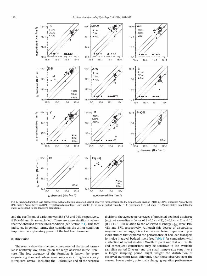
Fig. 5. Predicted unit bed load discharge by evaluated formulas plotted against observed rates according to the Armor Layer Division (ALD); i.e., UAL: Unbroken Armor Layer,BAL: Broken Armor Layer, and RAL: reestablished armor layer. Lines parallel to the line of perfect equality (r = 1) correspond to r = 0.1 and r = 10. Values plotted parallel to thex axis correspond to bed load zero predictions.

176 R. López et al. / Journal of Hydrology 510 (2014) 164–181

and the coefficient of variation was 88% (7.6 and 91%, respectively,if P–K–M and Bt are excluded). These are more significant valuesthat the obtained for the BMD condition (see Section 7.1). This factindicates, in general terms, that considering the armor conditionimproves the explanatory power of the bed load formulae.

8. Discussion

The results show that the predictive power of the tested formu-lae is relatively low, although on the range observed in the litera-ture. The low accuracy of the formulae is known by everyengineering standard, where commonly a much higher accuracyis required. Overall, including the 10 formulae and all the scenario

divisions, the average percentages of predicted bed load discharge(qsp) not exceeding a factor of 2 (0.5 < r < 2), 5 (0.2 < r < 5) and 10(0.1 < r < 10) in relation to the observed discharge (qso) were 19%,41% and 57%, respectively. Although this degree of discrepancymay seem rather large, it is not unreasonable in comparison to pre-vious studies that explored the performance of bed load transportformulae in gravel bedded rivers (see Table 8 for comparison witha selection of recent studies). Worth to point out that our resultsand consequent conclusions may be sensitive to the availablesampling period (2 years) and the small sample size (one river).A longer sampling period might weight the distribution ofobserved transport rates differently than those observed over thecurrent 2-year period, potentially changing equation performance.

1E-5

1E-4

1E-3

1E-2

1E-1

1E+0

1E+1

1E+2

1E+3

1E+4

S

MP

-M

W-P E-B

A-W B Y R

P-K

-M*

Bt*

Eq.

(5)

r = q

spr

edic

ted

/ qs

obse

rved

S

MP

- M

W-P E-B

A-W B Y R

P-K

-M*

Bt*

Eq.

(5)

75%Median

Max.

25%

Min.

S

MP

-M

W-P

E-B

A-W B Y R

P-K

-M**

Bt*

*

Eq.

(5)

Bed load Formula

1E-5

1E-4

1E-3

1E-2

1E-1

1E+0

1E+1

1E+2

1E+3

1E+4

1E-5

1E-4

1E-3

1E-2

1E-1

1E+0

1E+1

1E+2

1E+3

1E+4(a)

(b)

(c)

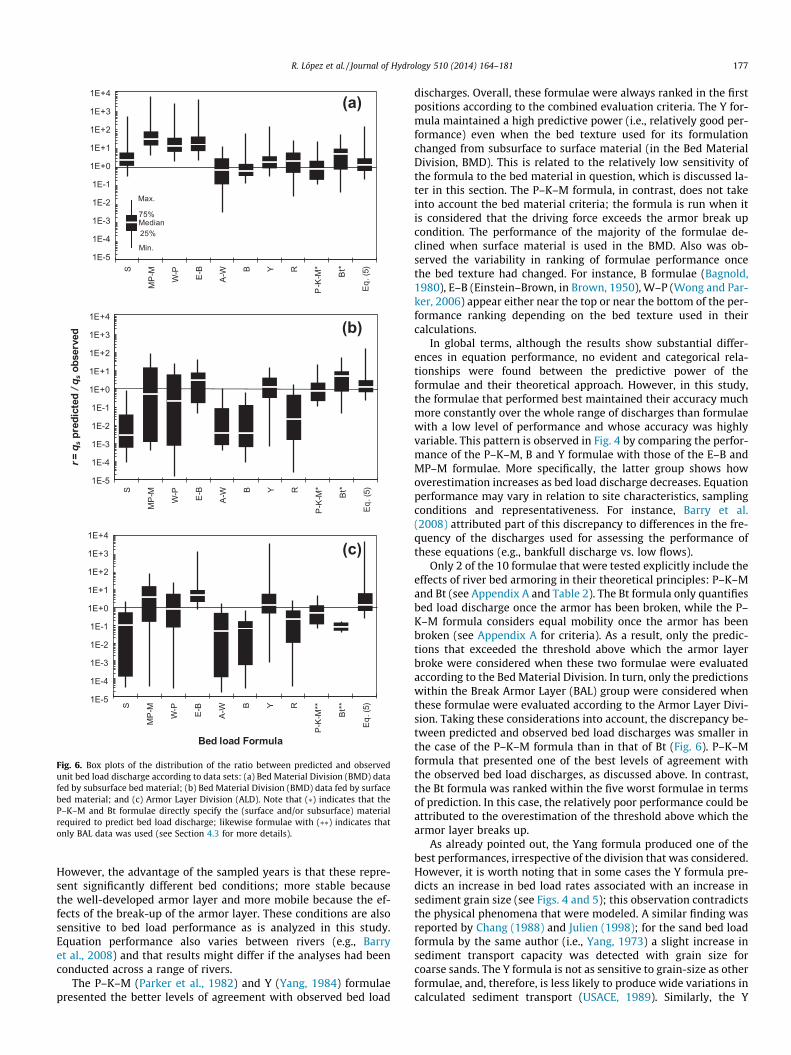
Fig. 6. Box plots of the distribution of the ratio between predicted and observedunit bed load discharge according to data sets: (a) Bed Material Division (BMD) datafed by subsurface bed material; (b) Bed Material Division (BMD) data fed by surfacebed material; and (c) Armor Layer Division (ALD). Note that (�) indicates that theP–K–M and Bt formulae directly specify the (surface and/or subsurface) materialrequired to predict bed load discharge; likewise formulae with (��) indicates thatonly BAL data was used (see Section 4.3 for more details).

R. López et al. / Journal of Hydrology 510 (2014) 164–181 177

However, the advantage of the sampled years is that these repre-sent significantly different bed conditions; more stable becausethe well-developed armor layer and more mobile because the ef-fects of the break-up of the armor layer. These conditions are alsosensitive to bed load performance as is analyzed in this study.Equation performance also varies between rivers (e.g., Barryet al., 2008) and that results might differ if the analyses had beenconducted across a range of rivers.

The P–K–M (Parker et al., 1982) and Y (Yang, 1984) formulaepresented the better levels of agreement with observed bed load

discharges. Overall, these formulae were always ranked in the firstpositions according to the combined evaluation criteria. The Y for-mula maintained a high predictive power (i.e., relatively good per-formance) even when the bed texture used for its formulationchanged from subsurface to surface material (in the Bed MaterialDivision, BMD). This is related to the relatively low sensitivity ofthe formula to the bed material in question, which is discussed la-ter in this section. The P–K–M formula, in contrast, does not takeinto account the bed material criteria; the formula is run when itis considered that the driving force exceeds the armor break upcondition. The performance of the majority of the formulae de-clined when surface material is used in the BMD. Also was ob-served the variability in ranking of formulae performance oncethe bed texture had changed. For instance, B formulae (Bagnold,1980), E–B (Einstein–Brown, in Brown, 1950), W–P (Wong and Par-ker, 2006) appear either near the top or near the bottom of the per-formance ranking depending on the bed texture used in theircalculations.

In global terms, although the results show substantial differ-ences in equation performance, no evident and categorical rela-tionships were found between the predictive power of theformulae and their theoretical approach. However, in this study,the formulae that performed best maintained their accuracy muchmore constantly over the whole range of discharges than formulaewith a low level of performance and whose accuracy was highlyvariable. This pattern is observed in Fig. 4 by comparing the perfor-mance of the P–K–M, B and Y formulae with those of the E–B andMP–M formulae. More specifically, the latter group shows howoverestimation increases as bed load discharge decreases. Equationperformance may vary in relation to site characteristics, samplingconditions and representativeness. For instance, Barry et al.(2008) attributed part of this discrepancy to differences in the fre-quency of the discharges used for assessing the performance ofthese equations (e.g., bankfull discharge vs. low flows).

Only 2 of the 10 formulae that were tested explicitly include theeffects of river bed armoring in their theoretical principles: P–K–Mand Bt (see Appendix A and Table 2). The Bt formula only quantifiesbed load discharge once the armor has been broken, while the P–K–M formula considers equal mobility once the armor has beenbroken (see Appendix A for criteria). As a result, only the predic-tions that exceeded the threshold above which the armor layerbroke were considered when these two formulae were evaluatedaccording to the Bed Material Division. In turn, only the predictionswithin the Break Armor Layer (BAL) group were considered whenthese formulae were evaluated according to the Armor Layer Divi-sion. Taking these considerations into account, the discrepancy be-tween predicted and observed bed load discharges was smaller inthe case of the P–K–M formula than in that of Bt (Fig. 6). P–K–Mformula that presented one of the best levels of agreement withthe observed bed load discharges, as discussed above. In contrast,the Bt formula was ranked within the five worst formulae in termsof prediction. In this case, the relatively poor performance could beattributed to the overestimation of the threshold above which thearmor layer breaks up.

As already pointed out, the Yang formula produced one of thebest performances, irrespective of the division that was considered.However, it is worth noting that in some cases the Y formula pre-dicts an increase in bed load rates associated with an increase insediment grain size (see Figs. 4 and 5); this observation contradictsthe physical phenomena that were modeled. A similar finding wasreported by Chang (1988) and Julien (1998); for the sand bed loadformula by the same author (i.e., Yang, 1973) a slight increase insediment transport capacity was detected with grain size forcoarse sands. The Y formula is not as sensitive to grain-size as otherformulae, and, therefore, is less likely to produce wide variations incalculated sediment transport (USACE, 1989). Similarly, the Y

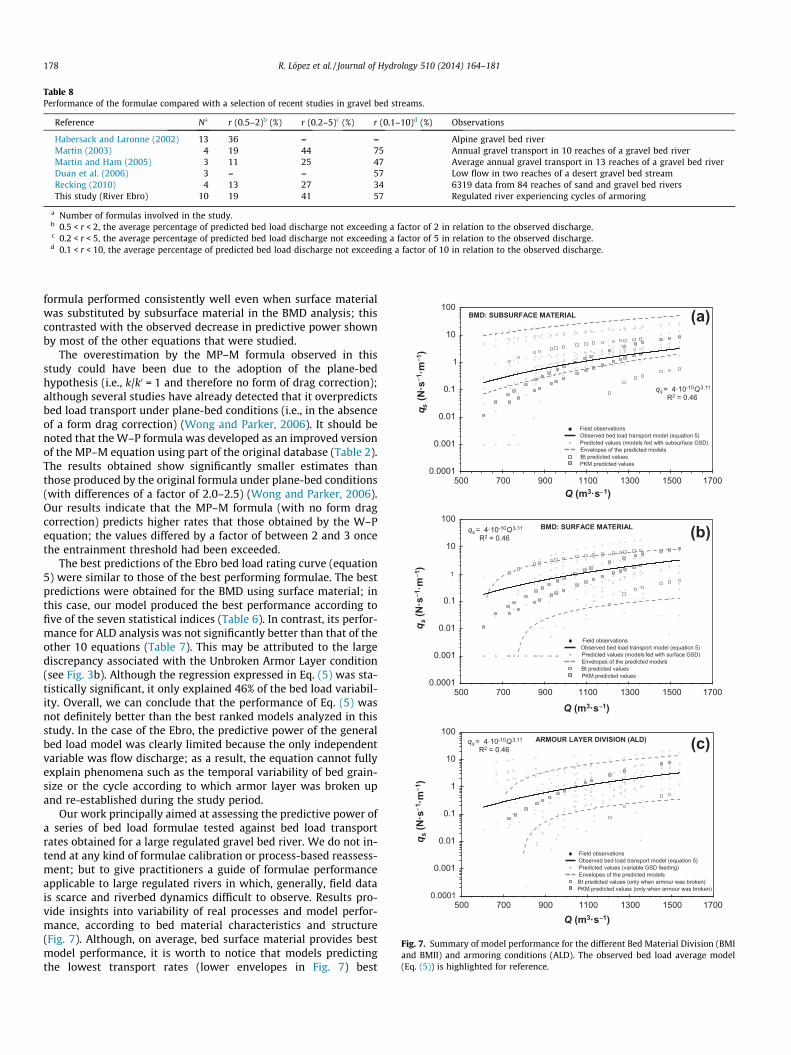
Table 8Performance of the formulae compared with a selection of recent studies in gravel bed streams.

Reference Na r (0.5–2)b (%) r (0.2–5)c (%) r (0.1–10)d (%) Observations

Habersack and Laronne (2002) 13 36 – – Alpine gravel bed riverMartin (2003) 4 19 44 75 Annual gravel transport in 10 reaches of a gravel bed riverMartin and Ham (2005) 3 11 25 47 Average annual gravel transport in 13 reaches of a gravel bed riverDuan et al. (2006) 3 – – 57 Low flow in two reaches of a desert gravel bed streamRecking (2010) 4 13 27 34 6319 data from 84 reaches of sand and gravel bed riversThis study (River Ebro) 10 19 41 57 Regulated river experiencing cycles of armoring

a Number of formulas involved in the study.b 0.5 < r < 2, the average percentage of predicted bed load discharge not exceeding a factor of 2 in relation to the observed discharge.c 0.2 < r < 5, the average percentage of predicted bed load discharge not exceeding a factor of 5 in relation to the observed discharge.d 0.1 < r < 10, the average percentage of predicted bed load discharge not exceeding a factor of 10 in relation to the observed discharge.

qs = 4·10-10Q3.11

R2 = 0.46

0.0001

0.001

0.01

0.1

1

10

100

500 700 900 1100 1300 1500 1700

0.0001

0.001

0.01

0.1

1

10

100

500 700 900 1100 1300 1500 1700

q s(N

·s1 ·m

1 )

Q (m3·s 1)

0.0001

0.001

0.01

0.1

1

10

100

500 700 900 1100 1300 1500 1700

BMD: SUBSURFACE MATERIAL

Field observationsObserved bed load transport model (equation 5)Predicted values (models fed with subsurface GSD)Envelopes of the predicted modelsBt predicted values PKM predicted values

Field observationsObserved bed load transport model (equation 5)Predicted values (models fed with surface GSD)Envelopes of the predicted modelsBt predicted values PKM predicted values

Field observationsObserved bed load transport model (equation 5)Predicted values (variable GSD feeding)Envelopes of the predicted modelsBt predicted values (only when armour was broken)PKM predicted values (only when armour was broken)

BMD: SURFACE MATERIAL

ARMOUR LAYER DIVISION (ALD)

Q (m3·s 1)

Q (m3·s 1)

q s(N

·s1 ·m

1 )q s

(N·s

1 ·m1 )

qs = 4·10-10Q3.11

R2 = 0.46

qs = 4·10-10Q3.11

R2 = 0.46

(a)

(b)

(c)

Fig. 7. Summary of model performance for the different Bed Material Division (BMIand BMII) and armoring conditions (ALD). The observed bed load average model(Eq. (5)) is highlighted for reference.

178 R. López et al. / Journal of Hydrology 510 (2014) 164–181

formula performed consistently well even when surface materialwas substituted by subsurface material in the BMD analysis; thiscontrasted with the observed decrease in predictive power shownby most of the other equations that were studied.

The overestimation by the MP–M formula observed in thisstudy could have been due to the adoption of the plane-bedhypothesis (i.e., k/k0 = 1 and therefore no form of drag correction);although several studies have already detected that it overpredictsbed load transport under plane-bed conditions (i.e., in the absenceof a form drag correction) (Wong and Parker, 2006). It should benoted that the W–P formula was developed as an improved versionof the MP–M equation using part of the original database (Table 2).The results obtained show significantly smaller estimates thanthose produced by the original formula under plane-bed conditions(with differences of a factor of 2.0–2.5) (Wong and Parker, 2006).Our results indicate that the MP–M formula (with no form dragcorrection) predicts higher rates that those obtained by the W–Pequation; the values differed by a factor of between 2 and 3 oncethe entrainment threshold had been exceeded.

The best predictions of the Ebro bed load rating curve (equation5) were similar to those of the best performing formulae. The bestpredictions were obtained for the BMD using surface material; inthis case, our model produced the best performance according tofive of the seven statistical indices (Table 6). In contrast, its perfor-mance for ALD analysis was not significantly better than that of theother 10 equations (Table 7). This may be attributed to the largediscrepancy associated with the Unbroken Armor Layer condition(see Fig. 3b). Although the regression expressed in Eq. (5) was sta-tistically significant, it only explained 46% of the bed load variabil-ity. Overall, we can conclude that the performance of Eq. (5) wasnot definitely better than the best ranked models analyzed in thisstudy. In the case of the Ebro, the predictive power of the generalbed load model was clearly limited because the only independentvariable was flow discharge; as a result, the equation cannot fullyexplain phenomena such as the temporal variability of bed grain-size or the cycle according to which armor layer was broken upand re-established during the study period.

Our work principally aimed at assessing the predictive power ofa series of bed load formulae tested against bed load transportrates obtained for a large regulated gravel bed river. We do not in-tend at any kind of formulae calibration or process-based reassess-ment; but to give practitioners a guide of formulae performanceapplicable to large regulated rivers in which, generally, field datais scarce and riverbed dynamics difficult to observe. Results pro-vide insights into variability of real processes and model perfor-mance, according to bed material characteristics and structure(Fig. 7). Although, on average, bed surface material provides bestmodel performance, it is worth to notice that models predictingthe lowest transport rates (lower envelopes in Fig. 7) best

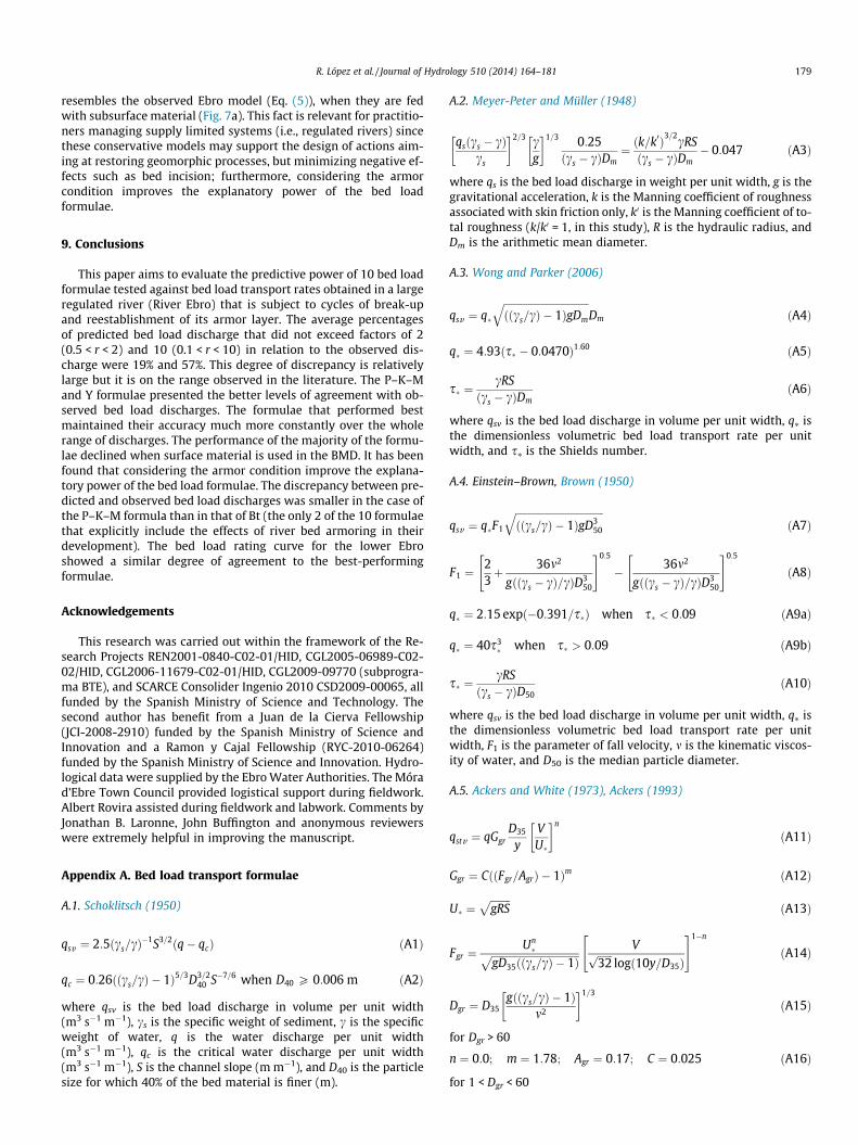
R. López et al. / Journal of Hydrology 510 (2014) 164–181 179

resembles the observed Ebro model (Eq. (5)), when they are fedwith subsurface material (Fig. 7a). This fact is relevant for practitio-ners managing supply limited systems (i.e., regulated rivers) sincethese conservative models may support the design of actions aim-ing at restoring geomorphic processes, but minimizing negative ef-fects such as bed incision; furthermore, considering the armorcondition improves the explanatory power of the bed loadformulae.

9. Conclusions

This paper aims to evaluate the predictive power of 10 bed loadformulae tested against bed load transport rates obtained in a largeregulated river (River Ebro) that is subject to cycles of break-upand reestablishment of its armor layer. The average percentagesof predicted bed load discharge that did not exceed factors of 2(0.5 < r < 2) and 10 (0.1 < r < 10) in relation to the observed dis-charge were 19% and 57%. This degree of discrepancy is relativelylarge but it is on the range observed in the literature. The P–K–Mand Y formulae presented the better levels of agreement with ob-served bed load discharges. The formulae that performed bestmaintained their accuracy much more constantly over the wholerange of discharges. The performance of the majority of the formu-lae declined when surface material is used in the BMD. It has beenfound that considering the armor condition improve the explana-tory power of the bed load formulae. The discrepancy between pre-dicted and observed bed load discharges was smaller in the case ofthe P–K–M formula than in that of Bt (the only 2 of the 10 formulaethat explicitly include the effects of river bed armoring in theirdevelopment). The bed load rating curve for the lower Ebroshowed a similar degree of agreement to the best-performingformulae.

Acknowledgements

This research was carried out within the framework of the Re-search Projects REN2001-0840-C02-01/HID, CGL2005-06989-C02-02/HID, CGL2006-11679-C02-01/HID, CGL2009-09770 (subprogra-ma BTE), and SCARCE Consolider Ingenio 2010 CSD2009-00065, allfunded by the Spanish Ministry of Science and Technology. Thesecond author has benefit from a Juan de la Cierva Fellowship(JCI-2008-2910) funded by the Spanish Ministry of Science andInnovation and a Ramon y Cajal Fellowship (RYC-2010-06264)funded by the Spanish Ministry of Science and Innovation. Hydro-logical data were supplied by the Ebro Water Authorities. The Mórad’Ebre Town Council provided logistical support during fieldwork.Albert Rovira assisted during fieldwork and labwork. Comments byJonathan B. Laronne, John Buffington and anonymous reviewerswere extremely helpful in improving the manuscript.

Appendix A. Bed load transport formulae

A.1. Schoklitsch (1950)

qsv ¼ 2:5ðcs=cÞ�1S3=2ðq� qcÞ ðA1Þ

qc ¼ 0:26ððcs=cÞ � 1Þ5=3D3=240 S�7=6 when D40 P 0:006 m ðA2Þ

where qsv is the bed load discharge in volume per unit width(m3 s�1 m�1), cs is the specific weight of sediment, c is the specificweight of water, q is the water discharge per unit width(m3 s�1 m�1), qc is the critical water discharge per unit width(m3 s�1 m�1), S is the channel slope (m m�1), and D40 is the particlesize for which 40% of the bed material is finer (m).

A.2. Meyer-Peter and Müller (1948)

qsðcs � cÞcs

� �2=3 cg

� �1=3 0:25ðcs � cÞDm

¼ ðk=k0Þ3=2cRSðcs � cÞDm

� 0:047 ðA3Þ

where qs is the bed load discharge in weight per unit width, g is thegravitational acceleration, k is the Manning coefficient of roughnessassociated with skin friction only, k0 is the Manning coefficient of to-tal roughness (k/k0 = 1, in this study), R is the hydraulic radius, andDm is the arithmetic mean diameter.

A.3. Wong and Parker (2006)

qsv ¼ q�ffiffiffiffiffiffiffiffiffiffiffiffiffiffiffiffiffiffiffiffiffiffiffiffiffiffiffiffiffiffiffiffiffiffiððcs=cÞ � 1ÞgDm

qDm ðA4Þ

q� ¼ 4:93ðs� � 0:0470Þ1:60 ðA5Þ

s� ¼cRS

ðcs � cÞDmðA6Þ

where qsv is the bed load discharge in volume per unit width, q⁄ isthe dimensionless volumetric bed load transport rate per unitwidth, and s⁄ is the Shields number.

A.4. Einstein–Brown, Brown (1950)

qsv ¼ q�F1

ffiffiffiffiffiffiffiffiffiffiffiffiffiffiffiffiffiffiffiffiffiffiffiffiffiffiffiffiffiffiffiffiffiffiffiððcs=cÞ � 1ÞgD3

50

qðA7Þ

F1 ¼23þ 36m2

gððcs � cÞ=cÞD350

" #0:5

� 36m2

gððcs � cÞ=cÞD350

" #0:5

ðA8Þ

q� ¼ 2:15 expð�0:391=s�Þ when s� < 0:09 ðA9aÞ

q� ¼ 40s3� when s� > 0:09 ðA9bÞ

s� ¼cRS

ðcs � cÞD50ðA10Þ

where qsv is the bed load discharge in volume per unit width, q⁄ isthe dimensionless volumetric bed load transport rate per unitwidth, F1 is the parameter of fall velocity, m is the kinematic viscos-ity of water, and D50 is the median particle diameter.

A.5. Ackers and White (1973), Ackers (1993)

qstv ¼ qGgrD35

yVU�

� �n

ðA11Þ

Ggr ¼ CððFgr=AgrÞ � 1Þm ðA12Þ

U� ¼ffiffiffiffiffiffiffiffigRS

pðA13Þ

Fgr ¼Un�ffiffiffiffiffiffiffiffiffiffiffiffiffiffiffiffiffiffiffiffiffiffiffiffiffiffiffiffiffiffiffiffiffiffiffi

gD35ððcs=cÞ � 1Þp Vffiffiffiffiffiffi

32p

logð10y=D35Þ

" #1�n

ðA14Þ

Dgr ¼ D35gððcs=cÞ � 1Þ

m2

� �1=3

ðA15Þ

for Dgr > 60

n ¼ 0:0; m ¼ 1:78; Agr ¼ 0:17; C ¼ 0:025 ðA16Þ

for 1 < Dgr < 60

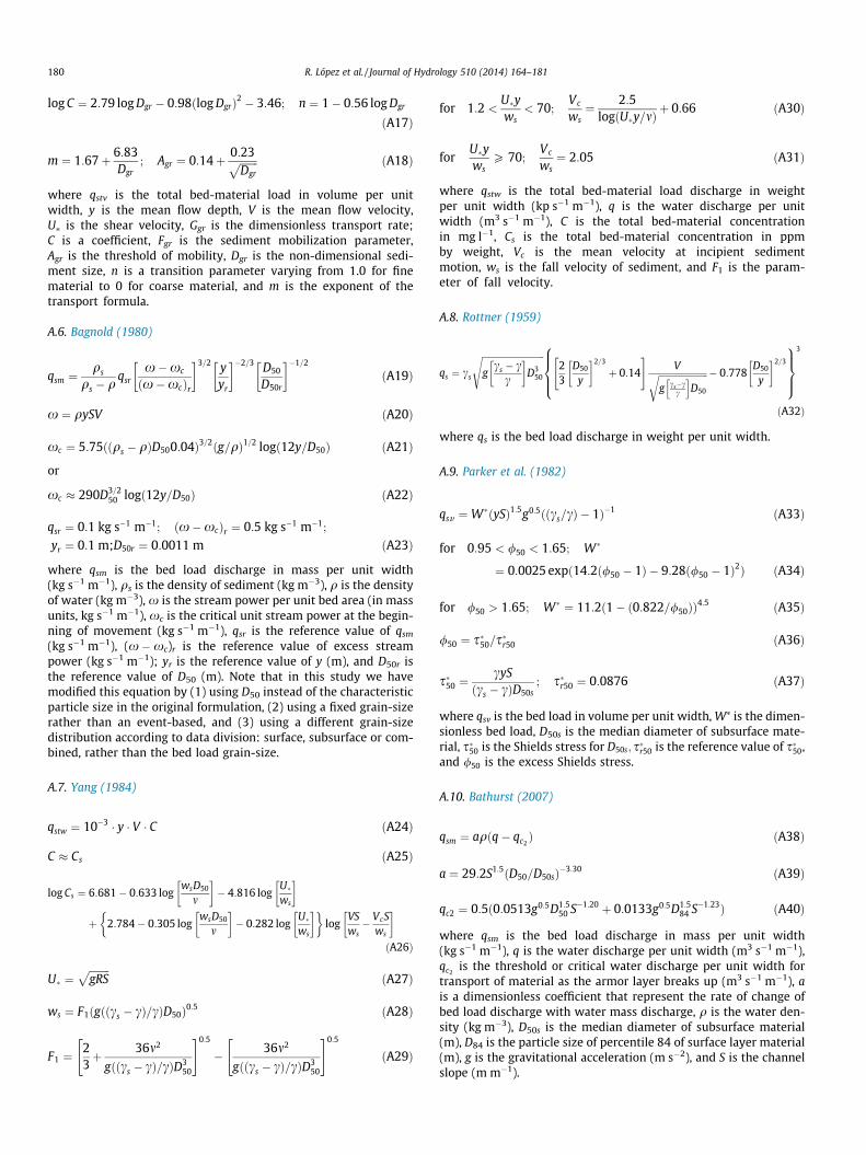
180 R. López et al. / Journal of Hydrology 510 (2014) 164–181

log C ¼ 2:79 log Dgr � 0:98ðlog DgrÞ2 � 3:46; n ¼ 1� 0:56 log Dgr

ðA17Þ

m ¼ 1:67þ 6:83Dgr

; Agr ¼ 0:14þ 0:23ffiffiffiffiffiffiffiDgr

p ðA18Þ

where qstv is the total bed-material load in volume per unitwidth, y is the mean flow depth, V is the mean flow velocity,U⁄ is the shear velocity, Ggr is the dimensionless transport rate;C is a coefficient, Fgr is the sediment mobilization parameter,Agr is the threshold of mobility, Dgr is the non-dimensional sedi-ment size, n is a transition parameter varying from 1.0 for finematerial to 0 for coarse material, and m is the exponent of thetransport formula.

A.6. Bagnold (1980)

qsm ¼qs

qs � qqsr

x�xc

ðx�xcÞr

� �3=2 yyr

� ��2=3 D50

D50r

� ��1=2

ðA19Þ

x ¼ qySV ðA20Þ

xc ¼ 5:75ððqs � qÞD500:04Þ3=2ðg=qÞ1=2 logð12y=D50Þ ðA21Þ

or

xc � 290D3=250 logð12y=D50Þ ðA22Þ

qsr ¼ 0:1 kg s�1 m�1; ðx�xcÞr ¼ 0:5 kg s�1 m�1;

yr ¼ 0:1 m;D50r ¼ 0:0011 m ðA23Þ

where qsm is the bed load discharge in mass per unit width(kg s�1 m�1), qs is the density of sediment (kg m�3), q is the densityof water (kg m�3), x is the stream power per unit bed area (in massunits, kg s�1 m�1), xc is the critical unit stream power at the begin-ning of movement (kg s�1 m�1), qsr is the reference value of qsm

(kg s�1 m�1), (x �xc)r is the reference value of excess streampower (kg s�1 m�1); yr is the reference value of y (m), and D50r isthe reference value of D50 (m). Note that in this study we havemodified this equation by (1) using D50 instead of the characteristicparticle size in the original formulation, (2) using a fixed grain-sizerather than an event-based, and (3) using a different grain-sizedistribution according to data division: surface, subsurface or com-bined, rather than the bed load grain-size.

A.7. Yang (1984)

qstw ¼ 10�3 � y � V � C ðA24Þ

C � Cs ðA25Þ

log Cs ¼ 6:681� 0:633 logwsD50

m

� �� 4:816 log

U�ws

� �

þ 2:784� 0:305 logwsD50

m

� �� 0:282 log

U�ws

� �� �log

VSws� VcS

ws

� �ðA26Þ

U� ¼ffiffiffiffiffiffiffiffigRS

pðA27Þ

ws ¼ F1ðgððcs � cÞ=cÞD50Þ0:5 ðA28Þ

F1 ¼23þ 36m2

gððcs � cÞ=cÞD350

" #0:5

� 36m2

gððcs � cÞ=cÞD350

" #0:5

ðA29Þ

for 1:2 <U�yws

< 70;Vc

ws¼ 2:5

logðU�y=mÞþ 0:66 ðA30Þ

forU�yws

P 70;Vc

ws¼ 2:05 ðA31Þ

where qstw is the total bed-material load discharge in weightper unit width (kp s�1 m�1), q is the water discharge per unitwidth (m3 s�1 m�1), C is the total bed-material concentrationin mg l�1, Cs is the total bed-material concentration in ppmby weight, Vc is the mean velocity at incipient sedimentmotion, ws is the fall velocity of sediment, and F1 is the param-eter of fall velocity.

A.8. Rottner (1959)

qs ¼ cs

ffiffiffiffiffiffiffiffiffiffiffiffiffiffiffiffiffiffiffiffiffiffiffiffiffiffiffiffig

cs � cc

� �D3

50

s23

D50

y

� �2=3

þ 0:14

" #Vffiffiffiffiffiffiffiffiffiffiffiffiffiffiffiffiffiffiffiffiffiffi

g cs�cc

h iD50

r � 0:778D50

y

� �2=3

8>><>>:

9>>=>>;

3

ðA32Þ

where qs is the bed load discharge in weight per unit width.

A.9. Parker et al. (1982)

qsv ¼W�ðySÞ1:5g0:5ððcs=cÞ � 1Þ�1 ðA33Þ

for 0:95 < /50 < 1:65; W�

¼ 0:0025 expð14:2ð/50 � 1Þ � 9:28ð/50 � 1Þ2Þ ðA34Þ

for /50 > 1:65; W� ¼ 11:2ð1� ð0:822=/50ÞÞ4:5 ðA35Þ

/50 ¼ s�50=s�r50 ðA36Þ

s�50 ¼cyS

ðcs � cÞD50s; s�r50 ¼ 0:0876 ðA37Þ

where qsv is the bed load in volume per unit width, W⁄ is the dimen-sionless bed load, D50s is the median diameter of subsurface mate-rial, s�50 is the Shields stress for D50s; s�r50 is the reference value of s�50,and /50 is the excess Shields stress.

A.10. Bathurst (2007)

qsm ¼ aqðq� qc2Þ ðA38Þ

a ¼ 29:2S1:5ðD50=D50sÞ�3:30 ðA39Þ

qc2 ¼ 0:5ð0:0513g0:5D1:550 S�1:20 þ 0:0133g0:5D1:5

84 S�1:23Þ ðA40Þ

where qsm is the bed load discharge in mass per unit width(kg s�1 m�1), q is the water discharge per unit width (m3 s�1 m�1),qc2

is the threshold or critical water discharge per unit width fortransport of material as the armor layer breaks up (m3 s�1 m�1), ais a dimensionless coefficient that represent the rate of change ofbed load discharge with water mass discharge, q is the water den-sity (kg m�3), D50s is the median diameter of subsurface material(m), D84 is the particle size of percentile 84 of surface layer material(m), g is the gravitational acceleration (m s�2), and S is the channelslope (m m�1).

R. López et al. / Journal of Hydrology 510 (2014) 164–181 181

References

Ackers, P., 1993. Sediment transport in open channels: Ackers and White update.Proc. Inst. Civil Eng. Water Marit. Energy 101, 247–249.

Ackers, P., White, W.R., 1973. Sediment transport: new approach and analysis. J.Hydraul. Div. 99 (11), 2041–2060.

Andrews, E.D., 1981. Measurement and computation of bed material discharge in ashallow sand-bed stream, Muddy Creek, Wyoming. Water Resour. Res. 17, 131–141.

Bagnold, R.A., 1980. An empirical correlation of bed load transport rates in flumesand natural rivers. Proc. Roy. Soc. Lond. Ser. A 372, 453–473.

Barry, J.J., Buffington, J.M., King, J.G., 2004. A general power equation for predictingbed load transport rates in gravel bed rivers. Water Resour. Res. 40, W10401.http://dx.doi.org/10.1029/2004WR003190.

Barry, J.J., Buffington, J.M., King, J.G., 2007. Correction to ‘‘A general power equationfor predicting bed load transport rates in gravel bed rivers’’. Water Resour. Res.43, W08702. http://dx.doi.org/10.1029/2007WR006103.

Barry, J.J., Buffington, J.M., Goodwin, P.G., King, J.G., Emmett, W.W., 2008.Performance of bed-load transport equations relative to geomorphicsignificance: predicting effective discharge and its transport rate. J. Hydraul.Eng. 134 (5), 601–615.

Batalla, R.J., 1997. Evaluating bed-material transport equations from fieldmeasurements in a sandy gravel-bed river. Earth Surf. Process. Land. 21, 121–130.

Batalla, R.J., Vericat, D., 2009. Hydrological and sediment transport dynamics offlushing flows: implications for management in large Mediterranean rivers.River Res. Appl. 25, 297–314.

Batalla, R.J., Gomez, C.M., Kondolf, G.M., 2004. Reservoir-induced hydrologicalchanges in the Ebro River basin (Northeastern Spain). J. Hydrol. 290 (1–2), 117–136.

Bathurst, J.C., 2007. Effect of coarse surface layer on bed-load transport. J. Hydraul.Eng. 133 (11), 1192–1205.

Brown, C.B., 1950. Sediment transportation. In: Rouse, H. (Ed.), Engineeringhydraulics. Wiley, New York, pp. 769–857.

Carson, M.A., Griffith, G.S., 1987. Bed load transport in gravel channels. J. Hydrol.(NZ) 26 (1), 1–151.

Casey, H.J., 1935. Über geschiebebewegung, Mitteilungen der PreussischenVersuchsanstalt. für Wasserbau und Schiffbau. 19, 86 pp.

Chang, Y.L., 1939. Laboratory investigation of flume traction and transportation.Trans. Am. Soc. Civil Eng. 104, 1246–1284.

Chang, H.H., 1988. Fluvial Processes in River Engineering. Wiley, New York.Chang, H.H., 1994. Selection of gravel-transport formula for stream modeling. J.

Hydraul. Eng. 120 (5), 646–651.Church, M., McLean, D.G., Wolcott, J.F., 1987. River bed gravels: sampling and

analysis. In: Thorne, C.R., Barthurst, J.C., Hey, R.D. (Eds.), Sediment Transport inGravel-bed Rivers. John Wiley and Sons, Chichester, UK, pp. 43–88.

Dietrich, W.E., Kirchner, J.W., Ikeda, H., Iseya, F., 1989. Sediment supply and thedevelopment of the coarse surface layer in gravel-bedded rivers. Nature 340,215–217.

Di Cristo, C., Iervolino, M., Vacca, A., 2006. Linear stability analysis of a 1-D modelwith dynamical description of bed-load transport. J. Hydraul. Res. 44 (4), 480–487.

Duan, J.G., Chen, L., Scott, S., 2006. Application of surface-based bed load transportequations to a desert gravel-bed stream. J. Hydraul. Res. 44 (5), 624–630.

Ferguson, R.I., 2003. The missing dimension: effects of lateral variation on 1-Dcalculations of fluvial bedload transport. Geomorphology 56, 1–14.

Fripp, J.B., Diplas, P., 1993. Surface sampling in gravel streams. J. Hydraul. Eng. 119(4), 473–490.

Gilbert, G.K., 1914. The transportation of débris by running water. U.S. GeologicalSurvey Professional Paper 86, 263 pp.

Gomez, B., 2006. The potential rate of bed-load transport. PNAS 103 (46), 17170–17173.

Gomez, B., Church, M., 1989. Assessment of bed load sediment transport formulaefor gravel bed rivers. Water Resour. Res. 25 (6), 1161–1186.

Greco, M., Iervolino, M., Leopardi, A., Vacca, A., 2012. A two-phase model for fastgeomorphic shallow flows. Int. J. Sediment. Res. 27 (4), 409–425.

Habersack, H., Laronne, J.B., 2002. Evaluation and improvement of bed loaddischarge formulas based on Helley–Smith sampling in an Alpine gravel bedriver. J. Hydraul. Eng. 128 (5), 484–499.

Hamamori, A., 1962. A Theoretical Investigation on the Fluctuations of Bed LoadTransport. Report R4, Delft Hydraulics Laboratory, Delft, The Netherlands, 14pp.

Johnson, J.W., 1939. Discussion of ‘Laboratory investigation of flume traction andtransportation’. Trans. Am. Soc. Civil Eng. 104, 1247–1313.

Julien, P.Y., 1998. Erosion and Sedimentation. Cambridge University Press, NewYork.

Kellerhals, R., Bray, D.I., 1971. Sampling procedures for coarse fluvial sediments. J.Hydraul. Div. 97 (8), 1165–1180.

Kramer, H., 1934. Sand mixtures and sand movements in fluvial models. Proc. Am.Soc. Civil Eng. 60 (4), 443–483.

Lane, E.W., Carlson, E.J., 1953. Some factors affecting the stability of canalsconstructed in coarse granular materials. In: Proceedings of the 5th CongressIAHR, Delf, The Netherlands.

López, R., Justribó, C., 2010. The hydrological significance of mountains: a regionalcase study, the Ebro River basin, northeast Iberian Peninsula. Hydrol. Sci. J. 55(2), 223–233.

Martin, Y., 2003. Evaluation of bed load transport formulae using field evidencefrom the Vedder River, British Columbia. Geomorphology 53, 75–95.

Martin, Y., Ham, D., 2005. Testing bed load transport formulae using morphologictransport estimates and field data: lower Fraser River, British Columbia. EarthSurf. Process. Land. 30, 1265–1282.

Meyer-Peter, E., Müller, R., 1948. Formulas for bed-load transport. In: Proc. 2ndMeeting of the Int. Assoc. for Hydraulic Structures Res. IAHR, Delft, TheNetherlands, pp. 39–64.

Parker, G., 1990. Surface-based bedload transport relation for gravel rivers. J.Hydraul. Res. 28, 417–436.

Parker, G., Klingeman, P.C., 1982. On why gravel bed streams are paved. WaterResour. Res. 18 (5), 1409–1423.

Parker, G., Klingeman, P.C., McLean, D.G., 1982. Bedload and the size distribution ofpaved gravel-bed streams. J. Hydraul. Div. 108 (4), 544–571.

Recking, A., 2010. A comparison between flume and field bed load transport dataand consequences for surface based bed load transport prediction. WaterResour. Res. 46, W03518. http://dx.doi.org/10.1029/2009WR008007.

Reid, I., Powell, D.M., Laronne, J.B., 1996. Prediction of bed load transport by desertflash-floods. J. Hydraul. Eng. 122 (3), 170–173.

Rice, S., Church, M., 1996. Sampling surficial fluvial gravels: the precision of sizedistribution percentile estimates. J. Sediment. Res. 66 (3), 654–665.

Rice, S.P., Haschenburger, J.K., 2004. A hybrid method for size characterization ofcoarse subsurface fluvial sediments. Earth Surf. Process. Land. 29, 373–389.

Rottner, J., 1959. A formula for bed load transportation. La Houille Blanche 3 (4),301–307.

Shields, A., 1936. Anwendung der Aehnlichkeitsmechanik und derTurbulenzforschung auf die Geschiebebewegung, Mitteilungen derPreussischen Versuchsanstalt für Wasserbau und Schiffbau, 26, 26 pp.

Schoklitsch, A., 1950. Handbuch des wasserbaues. Springer, New York.Shulits, S., Hill, R.D., 1968. Bed Load Formulas. Rep. No. ARSSCW-1, Agricultural

Research Services, USDA, Washington.Turowski, J.M., Badoux, A., Rickenmann, D., 2011. Start and end of bed load

transport in gravel-bed streams. Geophys. Res. Lett. 38, L04401.USACE, 1989. Sedimentation Investigations of Rivers and Reservoirs. Engineer

Manual 1110-2-4000. Department of the Army, U.S. Army Corps of Engineers,Washington.

USWES, 1935. Study of River-Bed Material and Their Use with Special Reference tothe Lower Mississippi River. United States Waterways Experiment Station,Vicksburg, MS, Paper 17, 161 pp.

Vericat, D., Batalla, R.J., 2005. Bed load variability under low sediment transportconditions in the lower Ebro River (NE Spain). In: Batalla, R.J., Garcia, C. (Eds.),Geomorphological Processes and Human Impacts in Rivers Basins. IAHSPublication, Wallingford, pp. 73–180.

Vericat, D., Batalla, R.J., 2006. Sediment transport in a large impounded river: thelower Ebro, NE Iberian Peninsula. Geomorphology 79, 72–92.

Vericat, D., Batalla, R.J., Garcia, C., 2006a. Breakup and reestablishment of the armorlayer in a highly regulated large gravel-bed river: the lower Ebro.Geomorphology 76, 122–136.

Vericat, D., Church, M., Batalla, R.J., 2006b. Bed load bias: comparison ofmeasurements obtained using two (76 and 152 mm) Helley–Smith samplersin a gravel-bed river. Water Resour. Res. W01402. http://dx.doi.org/10.1029/2005WR004025.

White, W.R., Milli, H., Crabbe, A.D., 1973. Sediment transport: an appraisal ofavailable methods, Rep. 119, UK Hydraulics Research Station, Wallingford, UK.

White, W.R., Milli, H., Crabbe, A.D., 1975. Sediment transport theories: a review.Proc. Inst. Civil Eng. 59 (2), 265–292.

Wilcock, P.R., 2001. The flow, the bed, and the transport: interaction in flume andfield. In: Mosley, M.P. (Ed.), Gravel-Bed Rivers V. NZHS, Wellington, NZ, pp. 183–219.

Wolman, M.G., 1954. A method of sampling coarse bed material. Am. Geophys.Union Trans. 35, 951–956.

Wong, M., Parker, G., 2006. Reanalysis and correction of bed-load relation of Meyer-Peter and Müller using their own database. J. Hydraul. Eng. 132 (11), 1159–1168.

Yang, C.T., 1973. Incipient motion and sediment transport. J. Hydraul. Div. 99 (10),1679–1704.

Yang, C.T., 1984. Unit stream power equation for gravel. J. Hydraul. Div. 110 (12),1783–1797.

Yang, C.T., Wan, S., 1991. Comparisons of selected bed-material load formulas. J.Hydraul. Eng. 117 (8), 973–989.