Evaluation of Background Metal Concentrations in Ohio … · Evaluation of Background Metal Concentrations in Ohio Soils June 21, 1996 Cox-Colvin & Associates, Inc. 2 across the state,

Evaluation of Background Metal Concentrations

in Ohio Soils

June 21, 1996

Submitted to:

Ohio Environmental Protection Agency1800 WaterMark Drive,

Columbus, Ohio 43266-0149

Submitted by:

Craig A. Cox, CPG George H. Colvin, CPG

Cox-Colvin & Associates, Inc.1151 Bethel Road, Suite 101

Columbus, Ohio 43220(614) 442-1970

Evaluation of Background Metal Concentrations in Ohio Soils June 21, 1996

Cox-Colvin & Associates, Inc. 1

Introduction

Soils contaminated by metals are common at many industrial sites in Ohio and across the country.The mere presence of metals in soils, however, does not necessarily indicate contamination becauseall soils naturally contain at least trace levels of metals (U.S. EPA, 1992a). The presence, nature,and extent of soil contamination by metals is commonly determined through comparisons of samplesfrom "affected" locations to those from "unaffected" locations at or near the site, or to publishedregional metal concentrations. These "unaffected" concentrations are commonly referred to asbackground. Background concentrations for naturally occurring constituents are used not only todetermine the presence, nature, and extent of contamination but also are used to aid in theestablishment of soil remediation goals. Such background-related evaluations are often requiredunder the Resource Conservation and Recovery Act (RCRA) and the Comprehensive EnvironmentalResponse, Compensation, and Liability Act (CERCLA).

In most cases, a direct statistical comparison to background data collected at a site is preferable overcomparison to regionally derived background levels. Site-specific background data are preferredbecause the concentration of metals in unaffected soil varies from location to location, dependingnot only on the geology of the parent material from which the soil was derived, but also on climaticconditions and local land use patterns. Despite the obvious advantages of direct statisticalcomparison to site specific background data, a simple comparison or, in some cases, a statisticalcomparison to regionally derived background data may be appropriate or even preferable in somesituations. For example, the lack of time or funding may prevent collection and analysis of sufficientbackground data. In other cases, it may be impossible to collect representative background data atan industrial facility due to limited space or the lack of an area unaffected by waste handling.

Published background metal concentrations in soils are available on a nation-wide level. Commonlycited references on this subject include Shacklette and Boerngen (1984), and Holmgren and others(1993). Whereas background soil data of this sort may be useful for making general comparisonsfrom one state or region to another, localized databases are preferable for focusing on environmentalobjectives such as determining whether or not a release has occurred or in developing remediationgoals. Logan and Miller published background levels for cadmium, chromium, copper, lead, nickel,and zinc from farm soil in seven counties in Ohio (Logan and Miller, 1983). While providing areasonable estimate of background metal concentrations for each of the seven counties, the limitedspatial variability of the data prevent adequate characterization of background for the state as awhole. Utilization of the Logan and Miller data is also limited by the number of metalscharacterized. Clearly, a more comprehensive data set is required to adequately characterize thevariation of background metal concentrations across the state. The primary objective of this study is to provide a state-wide statistical evaluation of backgroundmetal concentrations in Ohio soils, for use by industry, regulatory agencies, consultants and thegeneral public. This study utilizes background data collected from environmental investigations



across the state, and provides state-wide background concentrations for 20 metals. The assembleddata set is from 64 sites in 36 of Ohio’s 88 counties. Due to the individual nature of theenvironmental reports used throughout the study, many of the sites do not include analyses for all20 metals.

This study was conducted in association with the Ohio Environmental Protection Agency (OhioEPA) Division of Hazardous Waste Management. Involvement of the Ohio EPA in the project doesnot imply endorsement of the findings of the study by Ohio EPA nor should this report be construedas Ohio EPA guidance. No source of outside funding was used in the development of this report.

Metals in Background Soil

Nearly all of today’s soils have been affected to some extent by anthropogenic processes. Farm soil,for instance, may contain heavy metals associated with sewage sludge application (Logan and Miller,1983) and/or the direct application of fertilizers containing metals such as manganese, copper, zinc,boron, and potassium (Ohio Agricultural Guide, 1988). Soils in urban settings often contain elevatedlevels of metals related to fallout associated with the burning of fossil fuels and refuse for thegeneration of heat and power, or from other industrial sources. In addition, elevated concentrationsof lead have been documented along roadways (Holmgren, et.al., 1983).

As a result, soils used to characterize background within Ohio may have a subtle overprint of theseand other anthropogenic sources. This generalization certainly is true for background data collectedfrom areas within or surrounding industrial facilities. However, as demonstrated by this study,background data affected by industrial activities (termed industrially-impacted soil) in many casescan be separated from those background data that represent soil conditions present throughout muchof the state.

Background Data Set

Data used in this evaluation of background metal concentrations in Ohio soils were compiled frompublic Ohio EPA files for RCRA closure, RCRA Corrective Action, and CERCLA projects. OhioEPA Division of Hazardous Waste Management, Central Office coordinated the selection of thereports to be included in the study. All of the reports that contained background metals data wereconsidered for inclusion in the database. In several cases, specific sites were removed from thedatabase at the request of Ohio EPA District Offices based on the location of the backgroundsamples. Background data from 64 environmental projects conducted between 1984 and 1994 wereused in the study. A list of the sites and the associated metals utilized in the study is provided inTable 1. A total of 36 of the 88 counties in Ohio are represented in the study (Figure 1).



Data Entry

Metal concentration data were entered into a relational database using a database applicationdesigned specifically for this project. Because metal concentrations in soil may be dependent on anumber of variables (i.e., the local setting, the parent geologic material, depth, and land use history),the database file structure was designed so that evaluation by a number of criteria could be madeeasily. The criteria include geologic setting (DRASTIC hydrogeologic settings of Aller ,et al., 1987),grain size description, sample depth, Unified Soil Classification Scheme, United States SoilConservation Service classification, Standard Industrial Classifications (SIC) Codes, and geographicsetting (state, county, latitude and longitude). The available data entry fields associated with thedatabase are summarized on Table 2. Due to insufficient detail in many of the data reports, muchof this information was not available.

To aid the data entry process, real-time error checking on such items as U.S. EPA facilityidentification number, facility name, address, SIC Codes, analyte names and concentration units wereprovided in the form of lookup tables. This consideration minimized data entry errors and reducedthe database review time. In addition, an audit trail was developed that tied each analytical resultto the report from which it was taken. The audit trail enabled a check of the database entries againstthe source data, and will be useful for future workers who may wish to review source documents indetail concerning a particular site or metal.

All of these considerations were met through the commercially available relational database programParadox for DOS® (Version 4.0). The application developed was written in the Paradox ApplicationLanguage (PAL®). Data tables are easily exported to other popular software formats (dBASE®,Lotus 123®, and Quattro®), or as ASCII files.

Data Review and Preparation

Following data entry, the database was checked against the source documents for completeness andaccuracy. The database files were then copied prior to data reduction and statistical analysis. Thisensured that the original database would remain intact. The following steps were taken to preparethe data for statistical analysis:

1) Censored data (non-detects) that did not include a detection limit were removed fromthe database. It was not possible to substitute values for these censored data viagenerally accepted statistical techniques because the metal-specific detection limitsthat were reported varied widely within the database. Generally accepted statisticaltechniques that allow replacement of censored data assume that the data are from thesame site, same sampling episode and/or have a constant detection limit.



2) Censored data for which specific detection limits were reported were replaced by onehalf their respective detection limits and carried through the statistical analysis. Thismethod of manipulating censored data is a generally accepted practice and is the onlypractical method to deal with the numerous detection limits reported for each metal.In addition, the authors believed this approach to be more conservative than simplyreplacing the censored data point concentration by the reported detection limit.

3) The facility count for each metal (i.e. the number of facilities at which a specificmetal was analyzed) was then reviewed (Table 3). Boron, lithium, molybdenum,silicon, and tin, which were analytes at less than three separate sites, were notconsidered for further analysis in this study. It was felt that the current data sets forthese metals lack the desired spatial variability for this study.

4) The percentage of censored data associated with each metal was computed and ispresented also in Table 3. Because many statistical techniques are inappropriate fordata sets with a high percentage of censored data (U.S. EPA, 1992b; Gilbert, 1987;and Gibbons, 1994), metals with greater than 60% censored data were not consideredfor statistical analysis. Statistical methods that compensate for high percentages ofcensored data were not utilized in this study because of the wide range of detectionlimits reported per analyte. Metals screened from further statistical analysis due toa high percentage of censored data included antimony (97% censored data), selenium(78% censored data), silver (72% censored data), and thallium (73% censored data).Limited information, such as the range of detections, are provided for these metalsin summary tables (Table 5).

5) Metals that were not screened out include aluminum, arsenic, barium, beryllium,cadmium, chromium, cobalt, copper, iron, lead, manganese, mercury, nickel,potassium, vanadium and zinc. The database then was queried by metal andsubjected to statistical analysis.

Statistical Approach

Metal-specific data sets used in this study consist of hundreds of sample results, many times largerthan those of the typical environmental background study which usually contain less than ten sampleresults. In addition, because the sample results in this evaluation are from a variety of locationsacross the state the authors were working under the assumption that any data set could containmultiple populations, either as a result of geologic variability or as a result of anthropogenic sources.To effectively handle the large data sets and meet the assumption of multiple populations, the authorsused an iterative approach to statistical analysis which combined visual inspection through the useof probability plots, statistical analysis, and statistical modeling. These procedures are discussedbelow.



Visual Inspection - Probability Plots

Probability plots are an effective means of visually evaluating the normality of large data sets suchas those presented in this report. On a probability plot, a normally distributed data set will form astraight line. Probability plots can also be used to evaluate transformed data sets. For example, log-normally distributed data sets will plot as a straight line after they have been log-transformed.Procedures for construction of probability plots are provided by Gilbert (1987).

In addition to evaluating normality and log-normality, probability plots also have been used toevaluate the presence of multiple populations within data sets. This method has been usedsuccessfully for many years in geochemical exploration to locate ore bodies (Parslow, 1974; Sinclair,1974 and 1976), and more recently to formulate cleanup standards for contaminated soils(Fleischhauer and Korte, 1990). Multiple populations will form distinct straight-line segments ona probability plot provided each population is normally distributed. Where two populations overlap,an inflection point will form. This point, referred to as the "threshold point" by Fleischhauer andKorte (1990), represents the separation point between two populations. Through this method,populations can be identified and segregated from one another for further analysis. Segregation ofthe data will be partial where overlap exists; however, the statistical bias probably will remain small(Fleischhauer and Korte, 1990).

Upon initial inspection, it appeared that the data for barium, cadmium, chromium, copper, lead,mercury and zinc contained two distinct populations. It was assumed that the two populationsrepresent background and industrially-impacted soils rather than natural variation within thebackground population due to such things as parent material or sample depth. This assumption issupported by sample descriptions which describe the presence of man-made fill materials and therelatively high concentrations detected in the industrially-impacted soils population. In addition, thetwo populations would be expected in soils collected at industrial facilities.

To illustrate the use of probability plots, two normally distributed data sets are presented asfrequency distributions on Figure 2a. The data are plotted on a probability plot in Figure 2b. In thiscase, Population A may represent background conditions and Population B may representindustrially-impacted soils. An inflection point between the two populations represents the thresholdpoint separating the two populations. For comparison, Figure 2c is the frequency distribution of thezinc data set from this study. Figure 2d is the probability plot for zinc. The two populations areeasily discernable.

Metal-specific data sets that demonstrated characteristics of multiple populations were divided intotwo subsets for further analysis. The threshold values (Table 4) were used as the divider. Thepopulations that contained the higher concentrations were assumed to belong to the industrially-impacted soils population. The remaining data were considered to represent background.



Statistical Analysis

Once the data sets were evaluated visually and segregated as necessary, they were subjected tostatistical analysis to identify outliers, further assess their distribution and develop summarystatistics. Outliers were identified using the box-plot method (Iglewicz and Hoaglin, 1993). Toidentify outliers by this method, data sets were ranked and the quartiles Q1 and Q3 determined.Upper and lower fences "U" and "L", respectively were then defined as:

U = Q3 + k(Q3-Q1) and L = Q1 - k(Q3-Q1).

Values that fell outside the fences were identified as outliers. The value for the constant "k" usedin this study was 2.3, as recommended by Iglewicz and Hoaglin (1993) for larger data sets.

Following outlier identification, the data sets for each metal were analyzed to determine if they werenormally or log-normally distributed by determining its probability plot correlation coefficient(Filliben, 1975). The correlation coefficient can range between 0 and 1, with 1 being a perfectcorrelation. As data sets become larger the critical values generated by Filliben approach unity andthe method becomes very sensitive to the presence of outliers and censored data. To assess thesensitivity of the method to outliers, normality testing was completed on the data sets before andafter outlier removal as suggested by Barnett and Lewis (1978) and Iglewicz and Hoaglin (1993).

Current U.S. EPA (1992b) guidance for statistical analysis cautions against the removal of outliers.This is a response, in part, to the small size of most background data sets where the removal of oneor two data points could constitute the removal of as much as 25% of the data. In large data sets,where the expected percentage of outliers is 10% or greater, the removal of identified outliers is anacceptable practice (David Hoaglin, personal communication, 1996). Sensitivity analyses performedon the data sets containing outliers indicated that they should be removed from the data sets priorto statistical analysis. Removal of the outliers, which typically represented less than 3% of the dataset, improved the normality of the data sets, reduced the standard deviation and had little to no affecton the mean or median.

Standard statistical methods were then used to determine the median, mean, minimum, maximum,range, count (number of observation), variance, coefficient of variance, sample standard deviation,skewness, and kurtosis for each population. Once the statistical evaluation was completed, aninverse log-transformation was applied to the mean for the log-normally distributed metals toprovide an untransformed value. In this study, the inverse log-transformed mean also is referred toas the geometric mean.



Statistical Modeling

A statistical modeling technique was used by the authors to visually compare the goodness-of-fitbetween observed data sets and modeled data sets. The modeled data sets were generated using thesame mean, standard deviation and number of observations as that of the observed data. Once themodeled data set was generated, it was plotted on the probability plot along with the observed dataand the degree to which the sets matched was evaluated visually. This method was especially usefulin evaluating how well the calculated statistics (mean and standard deviation) characterized theobserved data in those data sets that contained outliers and/or a large percentage of censored data. In situations where multiple populations were identified, the statistical modeling technique was usedalso to refine the determination of the threshold point. Following an initial segregation and statisticalanalysis of the background and industrially-impacted soil data for a specific metal, the two modeleddata sets were added together, plotted on probability paper along side the original data and compared.Then a new threshold point was determined and the statistical analysis, modeling, and visualinspection repeated until the best curve match was obtained.

Data Presentation

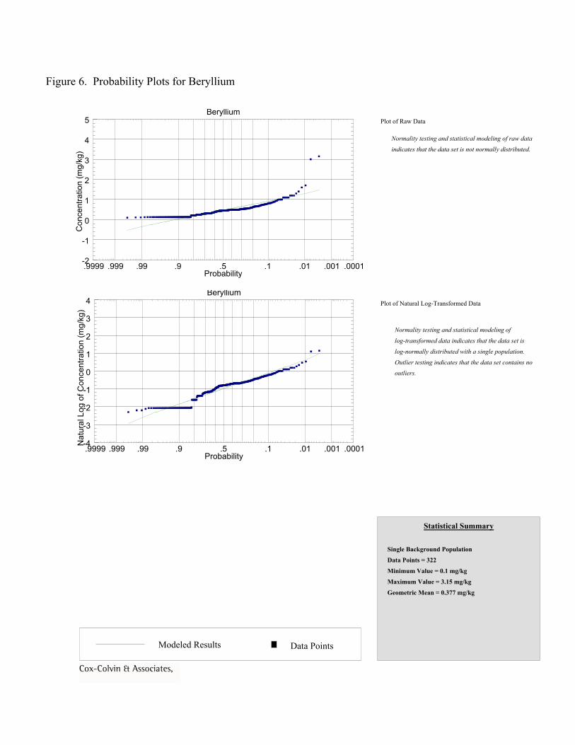
Probability plots for aluminum, arsenic, barium, beryllium, cadmium, chromium, cobalt, copper,iron, lead, manganese, mercury, nickel, potassium, vanadium and zinc are presented on Figures 3through 18. These figures represent as many as three probability plots for each metal. The first plotin each case is of the raw (untransformed) data; the second is of the natural log-transformed data,and, where appropriate, the third plot represents the natural log-transformed data that has beencorrected for outliers. Outliers and threshold points have been identified on the plots. Except foraluminum, each of these metals is log-normally distributed. Aluminum appears to be normallydistributed. Data sets for barium, cadmium, chromium, copper, lead, mercury, and zinc weredetermined to contain two populations.

The results of the statistical evaluations of background soils for Ohio are presented in Table 5 andthose for industrially-impacted soil are presented in Table 6. The results are provided on a metal bymetal basis. The tables include the following information for each of the metals: count (number ofdata points), minimum and maximum concentration, range, variance, coefficient of variance,standard deviation, standard error, skewness, kurtosis, mean, median and geometric mean. Asummary of statistical results is provided also on the probability plots (Figures 3 through 18). Thestatistical summaries for industrially-impacted soil have been presented in this report because: 1)they were identified as separate and distinct populations not related to background and 2) todocument the statistical approach used in this study. Because the focus of the investigations thatgenerated the data used in this study was to evaluate background conditions (not industrially-impacted conditions), the authors caution against the use of the industrially-impacted soil statisticalsummaries.



Because of the log-normal distribution of the data, mean values are provided as geometric means forall metals with the exception of aluminum. The arithmetic mean is used for aluminum. Shackletteand Boerngen (1984) note that trace metals tend to have positively skewed frequency distributions,and thus the geometric mean is the more proper measure of central tendency for most elements insoils. Shacklette and Boerngen (1984) also note that the frequency distribution for aluminum usuallyis normal if the data are not log-transformed and the mean is expressed as the arithmetic mean.

Discussion of Results

The results of the statistical evaluation of background metal concentrations for soils in the state ofOhio are discussed below, in alphabetical order. The discussion is limited to state-wide occurrencesof metals in background and, where appropriate, in industrially-impacted soil. In addition, wherepossible, the results determined in this study are compared (Table 7) to those of previousinvestigators including Brooks (1972), Logan and Miller (1983), Shacklette and Boerngen (1984),and Holmgren and others (1993). The statistical results developed by Logan and Miller (1983) andHolmgren and others (1993) are for Ohio, whereas those from the Shacklette and Boerngen (1984),and Brooks (1972) are for the eastern United States (east of the 96th meridian), and the UnitedStates, respectively.

Aluminum

A total of 136 aluminum determinations associated with four sites in four counties exist in thecurrent database. None of these determinations were reported as being below the detection limit(Table 3). The data were found to be normally distributed with a single background population(Figure 3). The background aluminum values range from 2,000 to 16,100 mg/kg, with a median of7,685 mg/kg and an arithmetic mean of 8,180 mg/kg (Table 5). Shacklette and Boerngen (1984)report a geometric mean of 33,000 mg/kg and a range of 7,000 mg/kg to 100,000 mg/kg for soilsof the eastern United States.

Antimony

A total of 285 antimony determinations associated with 10 sites in nine counties exist in the currentdatabase. Of these, 276 (97%) were reported as being below the detection limit (Table 3). Due tothe large amount of censored data, antimony data were not evaluated statistically. Detected levelsof antimony range from 0.97 to 92 mg/kg (Table 5). Detection limits range from 0.30 to 15 mg/kg.The most frequently occurring detection limit was 5 mg/kg. At these detection limits, it appears thatantimony is not typically detected in Ohio soils. Shacklette and Boerngen (1984) report a geometricmean of 0.52 mg/kg and a range of <1 mg/kg to 8.8 mg/kg for soils of the eastern United States.Brooks (1972) reports an average of 0.5 mg/kg for U.S. soils.



Arsenic

A total of 693 arsenic determinations associated with 32 sites in 22 counties exist in the currentdatabase. Of these, 46 (7%) were reported as being below the detection limit (Table 3). The datawere found to be log-normally distributed within a single background population (Figure 4). Outliertesting indicated that the data set contains seven outliers. After the removal of three high value andfour low value outliers, the data set ranges from 0.50 mg/kg to 56 mg/kg, with a median of 5.80 anda geometric mean of 5.72 mg/kg (Table 5). Shacklette and Boerngen (1984) report a geometric meanof 4.8 mg/kg and a range of <0.1 mg/kg to 73 mg/kg for soils of the eastern United States. Brooks(1972) reports an average of 5 mg/kg for U.S. soils.

Barium

A total of 742 barium determinations associated with 37 sites in 24 counties exist in the currentdatabase. Of these, 4 (0.5%) were reported as being below the detection limit (Table 3). The datawere found to be log-normally distributed with both a background population and an industrially-impacted soil population (Figure 5). Outlier testing indicated that the data set contains seven lowvalue outliers. Statistical modeling indicated that the natural log of the threshold value whichseparates the populations to be 5.80. This value equates to 330 mg/kg (Table 4).

The background data set contains 710 observations. The background values range from 9.3 mg/kgto 323 mg/kg with a median of 63.2 and a geometric mean of 63.4 mg/kg (Table 5). Shacklette andBoerngen (1984) report a geometric mean of 290 mg/kg and a range of 10 mg/kg to 1,500 mg/kg forU.S. soils. Brooks (1972) reports an average of 500 mg/kg for U.S. soils.

The industrially-impacted soil data set contains 25 observations with values ranging from 331 mg/kgto 7,790 mg/kg with a median of 660 mg/kg and a geometric mean of 838 mg/kg (Table 6).

Beryllium

A total of 322 beryllium determinations associated with eight sites in seven counties exist in thecurrent database. Of these, 115 (36%) were reported as being below the detection limit (Table 3).The data were found to be log-normally distributed within a single background population (Figure6). The values range from 0.10 mg/kg to 3.15 mg/kg with a median of 0.450 mg/kg and a geometricmean of 0.377 mg/kg (Table 5). Shacklette and Boerngen (1984) report a geometric mean of 0.55mg/kg and a range of <1 mg/kg to 7 mg/kg for soils of the eastern United States. Brooks (1972)reports an average of 6 mg/kg for U.S. soils.



Cadmium

A total of 768 cadmium determinations associated with 44 sites in 28 counties exist in the currentdatabase. Of these, 397 (52%) were reported as being below the detection limit (Table 3). The datawere found to be log-normally distributed with both a background population and an industrially-impacted soil population (Figure 7). Outlier testing indicates that the data set contains three lowvalue outliers. Statistical modeling indicates that the natural log of the threshold value whichseparates the populations is 1.5. This value equates to 4.5 mg/kg (Table 4).

The background data set contains 706 observations. The background values range from 0.07 to 4.4mg/kg with a median of 0.480 and a geometric mean of 0.507 mg/kg (Table 5). Logan and Miller(1983) report a mean of 0.2 mg/kg and a range of below detection to 2.9 mg/kg. Holmgren andothers (1993) reports a geometric mean of 0.357 mg/kg for Ohio soils.

The industrially-impacted soil data set contains 59 observations with values ranging from 4.50 mg/kgto 362 mg/kg with a median of 12.0 and a geometric mean of 13.0 mg/kg (Table 6).

Chromium

A total of 972 chromium determinations associated with 50 sites in 31 counties exist in the currentdatabase. Of these, 23 (3%) were reported as being below the detection limit (Table 3). The datawere found to be log-normally distributed with both a background population and an industrially-impacted soil population (Figure 8). Outlier testing indicates that the data set contains 15 low valueoutliers. Statistical modeling indicates that the natural log of the threshold value which separatesthe populations is 4.4. This value equates to 81 mg/kg (Table 4).

The background data set contains 925 observations. The background values range from 2.0 to 80.5mg/kg with a median of 12.0 mg/kg and a geometric mean of 12.1 mg/kg (Table 5). Logan andMiller (1983) report a mean of 12 mg/kg and a range of 4 to 23 mg/kg for Ohio soils. Shacklette andBoerngen (1984) report a geometric mean of 33 mg/kg and a range of 1 to 1,000 mg/kg for soils ofthe eastern United States. Brooks (1972) reports an average of 200 mg/kg for U.S. soils.

The industrially-impacted soil data set contains 32 observations with values ranging from 83.2 mg/kgto 2,340 mg/kg with a median of 200 mg/kg and a geometric mean of 260 mg/kg (Table 6).

Cobalt

A total of 320 cobalt determinations associated with seven sites in six counties exist in the currentdatabase. Of these, 24 (8%) were reported as being below the detection limit (Table 3). The datawere found to be log-normally distributed within a single background population (Figure 9). Outliertesting indicates that the data set contains three low value outliers. The background values range



from 1.0 to 53.6 mg/kg with a median of 7.25 mg/kg and a geometric mean of 6.42 mg/kg (Table5). Shacklette and Boerngen (1984) report a geometric mean of 5.9 mg/kg and a range of <0.3mg/kg to 70 mg/kg for soils of the eastern United States. Brooks (1972) reports an average of 10mg/kg for U.S. soils.

Copper

A total of 392 copper determinations associated with 13 sites in 12 counties exist in the currentdatabase. Of these, 2 (0.5%) were reported as being below the detection limit (Table 3). The datawere found to be log-normally distributed with both a background population and an industrially-impacted soil population (Figure 10). Outlier testing indicates that the data set contains one lowvalue outlier. Statistical modeling indicates that the natural log of the threshold value whichseparates the populations is 4.1. This value equates to 60 mg/kg (Table 4).

The background data set contains 357 observations. The background values range from 2.2 mg/kgto 58 mg/kg with a median of 12.0 mg/kg and a geometric mean of 11.8 mg/kg (Table 5). Logan andMiller (1983) report a mean of 19 mg/kg and a range of 11 to 37 mg/kg for Ohio soils. Holmgrenand others (1993) reports a geometric mean of 26.2 mg/kg for Ohio soils. Shacklette and Boerngen(1984) report a geometric mean of 13 mg/kg and a range of <1 mg/kg to 700 mg/kg for soils of theeastern United States. Brooks (1972) reports an average of 20 mg/kg for U.S. soils.

The industrially-impacted soil data set contains 34 observations with values ranging from 66 mg/kgto 1,420 mg/kg with a median of 236 and a geometric mean of 233 mg/kg (Table 6).

Iron

A total of 156 iron determinations associated with four sites in four counties exist in the currentdatabase. Of these, 0 (0%) were reported as being below the detection limit (Table 3). The datawere found to be log-normally distributed within a single background population (Figure 11).Outlier testing indicates that the data set contains one low value outlier. The background valuesrange from 5,150 to 100,000 mg/kg with a median of 17,300 mg/kg and a geometric mean of 18,400mg/kg (Table 5). Shacklette and Boerngen (1984) report a geometric mean of 14,000 mg/kg and arange of 100 to 100,000 mg/kg for soils of the eastern United States. Brooks (1972) reports a rangeof 10,000 to 50,000 mg/kg for U.S. soils.

Lead

A total of 1,019 lead determinations associated with 56 sites in 32 counties exist in the currentdatabase. Of these, 76 (7%) were reported as being below the detection limit (Table 3). The datawere found to be log-normally distributed with both a background population and an industrially-impacted soil population (Figure 12). Outlier testing indicates that the data set contains four low



value outliers. Statistical modeling indicates that the natural log of the threshold value whichseparates the populations is 5.0. This value equates to 148 mg/kg (Table 4).

The background data set contains 929 observations. The background values range from 1.0 mg/kgto 147 mg/kg with a median of 14.3 and a geometric mean of 16.2 mg/kg (Table 5). Logan andMiller (1983) report a mean of 19 mg/kg and a range of 9 to 39 mg/kg for Ohio soils. Holmgren andothers (1993) reports a geometric mean of 18.2 mg/kg for Ohio soils. Shacklette and Boerngen(1984) report a geometric mean of 14 mg/kg and a range of <10 mg/kg to 300 mg/kg for soils of theeastern United States. Brooks (1972) reports an average of 10 mg/kg for U.S. soils.

The industrially-impacted soil data set contains 86 observations with values ranging from 152 mg/kgto 10,500 mg/kg with a median of 558 and a geometric mean of 633 mg/kg (Table 6).

Manganese

A total of 124 manganese determinations associated with three sites in three counties exist in thecurrent database. Of these, 0 (0%) were reported as being below the detection limit (Table 3). Thedata were found to be log-normally distributed within a single background population (Figure 13).Outlier testing indicates that the data set contains three low value outliers and one high value outlier.Background values range from 59 to 1,750 mg/kg with a median of 476 mg/kg and a geometric meanof 459 mg/kg (Table 5). Shacklette and Boerngen (1984) report a geometric mean of 260 mg/kg anda range of <2 to 7,000 mg/kg for soils of the eastern United States. Brooks (1972) reports an averageof 850 mg/kg for U.S. soils.

Mercury

A total of 580 mercury determinations associated with 29 sites in 20 counties exist in the currentdatabase. Of these, 331 (57%) were reported as being below the detection limit (Table 3). The datawere found to be log-normally distributed with both a background population and an industrially-impacted soil population (Figure 14). Outlier testing indicates that the data set contains 22 low valueoutliers. Statistical modeling indicates that the natural log of the threshold value which separatesthe populations is 0.5. This value equates to 1.6 mg/kg (Table 4).

The background data set contains 514 observations. The values range from 0.010 mg/kg to 1.6mg/kg with a median of 0.060 mg/kg and a geometric mean of 0.081 mg/kg (Table 5). Shackletteand Boerngen (1984) report a geometric mean of 0.081 mg/kg and a range of 0.01 to 3.4 mg/kg forsoils of the eastern United States. Brooks (1972) reports an average of 0.01 mg/kg for U.S. soils.

The industrially-impacted soil data set contains 44 observations with values ranging from 1.8 to 96mg/kg with a median of 18.8 mg/kg and a geometric mean of 10.7 mg/kg (Table 6).



Nickel

A total of 555 nickel determinations associated with 20 sites in 17 counties exist in the currentdatabase. Of these, 28 (5%) were reported as being below the detection limit (Table 3). The datawere found to be log-normally distributed within a background population (Figure 15). Outliertesting indicates that the data set contains four low value outliers and three high value outliers. Thebackground values range from 2.0 mg/kg to 110 mg/kg with a median of 14.7 and a geometric meanof 14.4 mg/kg (Table 5). Logan and Miller (1983) report a mean of 18 mg/kg and a range of 9 mg/kgto 38 mg/kg for Ohio soils. Holmgren and others (1993) report a geometric mean of 27.1 mg/kg forOhio soils. Shacklette and Boerngen (1984) report a geometric mean of 11 mg/kg and a range of <5to 700 mg/kg for soils of the eastern United States. Brooks (1972) reports an average of 40 mg/kgfor U.S. soils.

Potassium

A total of 145 potassium determinations associated with four sites in four counties exist in thecurrent database. Of these, 8 (6%) were reported as being below the detection limit (Table 3). Thedata were found to be log-normally distributed within a single background population (Figure 16).The values range from 230 to 2,180 mg/kg with a median of 720 mg/kg and a geometric mean of 709mg/kg (Table 5). Shacklette and Boerngen (1984) report an arithmetic mean of 12,000 mg/kg anda range of 50 to 37,000 mg/kg for soils of the eastern United States.

Selenium

A total of 480 selenium determinations associated with 23 sites in 18 counties exist in the currentdatabase. Of these, 376 (78%) were reported as being below the detection limit (Table 3). Due tolarge amount of censored data, these data were not evaluated statistically. Detected values rangefrom 0.2 to 35 mg/kg (Table 5). Detection limits for selenium range from 0.003 mg/kg to 5 mg/kg.The most frequently occurring detection limit is 0.25 mg/kg. At these detection limits it appears thatselenium is not typically detected in Ohio soils. Shacklette and Boerngen (1984) report a geometricmean of 0.30 mg/kg and a range of <0.1 to 3.9 mg/kg for soils of the eastern United States. Brooks(1972) reports an average of 0.5 mg/kg for U.S. soils.

Silver

A total of 433 silver determinations associated with 20 sites in 17 counties exist in the currentdatabase. Of these, 313 (72%) were reported as being below the detection limit (Table 3). Due tolarge amount of censored data, these data were not evaluated statistically. Detected values rangefrom 0.2 to 14.8 mg/kg (Table 5). Detection limits for silver range from 0.03 to 2.5 mg/kg. Themost frequently occurring detection limit is 0.25 mg/kg. At these detection limits it appears thatsilver is not typically detected in Ohio soils. Limited published background data for silver are



available. U.S. EPA (1983) cite a common range of 0.01 to 5 mg/kg and an average of 0.05 mg/kgfor U.S. soils.

Thallium

A total of 276 thallium determinations associated with six sites in six counties exist in the currentdatabase. Of these, 201 (73%) were reported as being below the detection limit (Table 3). Due tothe large amount of censored data, these data were not evaluated statistically. Detected values rangefrom 0.17 to 0.59 mg/kg (Table 5). Detection limits for thallium range from 0.16 to 2.5 mg/kg. Themost frequent detection limit is 2.5 mg/kg. At these detection limits it appears that thallium is nottypically detected in Ohio soils. Shacklette and Boerngen (1984) report a geometric mean of 7.7mg/kg and a range of 2.2 to 23 mg/kg for soils of the eastern United States. Brooks (1972) reportsan average of 13 mg/kg for U.S. soils.

Vanadium

A total of 367 vanadium determinations associated with nine sites in eight counties exist in thecurrent database. Of these, 0 (0%) were reported as being below the detection limit (Table 3). Thedata were found to be log-normally distributed within a single background population (Figure 17).The values range from 4.6 to 71 mg/kg with a median of 17.8 mg/kg and a geometric mean of 17.4mg/kg (Table 5). Shacklette and Boerngen (1984) report a geometric mean of 43 mg/kg and a rangeof <7 mg/kg to 300 mg/kg for soils of the eastern United States. Brooks (1972) reports an averageof 100 mg/kg for U.S. soils.

Zinc

A total of 472 zinc determinations associated with 17 sites in 16 counties exist in the currentdatabase. Of these, 9 (2%) were reported as being below the detection limit (Table 3). The datawere found to be log-normally distributed with both a background population and an industrially-impacted soil population (Figure 18). Outlier testing indicates that the data set contains one lowvalue outlier and two high value outliers. Statistical modeling indicates that the natural log of thethreshold value which separates the populations is 5.30. This value equates to 200 mg/kg (Table 4). The background data set contains 434 observations. The background values range from 7.5 mg/kgto 190 mg/kg with a median of 43.0 mg/kg and a geometric mean of 42.7 mg/kg (Table 5). Loganand Miller (1983) report a mean of 75 mg/kg and a range of 47 mg/kg to 138 mg/kg for Ohio soils.Holmgren and others (1993) report a geometric mean of 82.1 mg/kg for Ohio soils. Shacklette andBoerngen (1984) report a geometric mean of 40 mg/kg and a range of <5 to 2,900 mg/kg for soilsof the eastern United States. Brooks (1972) reports an average of 50 mg/kg for U.S. soils.



The industrially-impacted soil data set contains 35 observations with values ranging from 210 to3,940 mg/kg with a median of 600 mg/kg and a geometric mean of 564 mg/kg (Table 6).

Conclusions

Background soil data from environmental investigations at 64 facilities in 36 of Ohio’s 88 countieswere used to assess the distribution of background metal concentrations in soils. The resultingdatabase, which contains over 10,000 separate analytical results for 20 metals, provides the mostcomprehensive collection of background soil quality data ever assembled for the state of Ohio.

Through the use of probability plots, statistical analysis and statistical modeling it was determinedthat, with the exception of aluminum, all of the metal concentrations in background soils evaluatedare log-normally distributed. Aluminum concentrations were found to be normally distributed.These findings agree with those of earlier investigators including Shacklette and Boerngen (1984)and Holmgren and others (1993). Multiple populations representing background and industrially-impacted soils were identified through the use of probability plots. Threshold values separating thetwo populations were determined through statistical modeling.

Aluminum, arsenic, beryllium, cobalt, iron, manganese, nickel, potassium, and vanadiumconcentrations were determined to belong to a single background population. However, barium,cadmium, chromium, copper, lead, mercury, nickel, and zinc concentrations were determined tobelong to two populations: background and industrially-impacted soil. Statistical summaries forindustrially-impacted soil have been presented in this report because: 1) they were identified asseparate and distinct populations not related to background and 2) to document the statisticalapproach used in this study. Because the focus of the investigations that generated the data used inthis study was to evaluate background conditions (not industrially-impacted conditions), the authorscaution against the use of the industrially-impacted soil statistical summaries.

The analytical results for antimony, selenium, silver, and thallium contained such a high percentageof censored data that the data could not be evaluated using standard parametric methods. Thegeneral lack of detectable concentrations does indicate, however, that these analytes are notcommonly detected in Ohio soils.

Within the two major populations (background and industrially-impacted soil) it is possible thatother, more subtle populations (i.e., those related to regional geological variability) may be present.Initially, it was hoped that these minor populations could be identified and characterized by soil type,DRASTIC hydrogeologic settings, glaciated versus non-glaciated locations, and/or grain size.However, such detail was not presented in many of the data reports utilized in this evaluation. Forthat reason, it was decided that background information would be provided on a state-wide basis foreach of the two major populations. In the future, as more data are included in the database, it is



anticipated that an increase in sample-specific detail will permit a statistical separation of specificgeologic settings.

Acknowledgments

The authors would like to thank Ohio EPA for their assistance and enthusiastic support of thisproject, for reviewing and commenting on draft versions of this document, and for providing internsto assist in data entry. Similarly, we would thank Mr. Joe Oiler and Ms. Laurie Chilcote for theirdiligent data entry efforts. We would also like to thank Dr. Douglas Pride, Dr. Christena Cox, Dr.Marcia Warner, James Warner, and Dr. Jennifer Heath for their critical review and comment on draftversions of this document. Lastly, we would like to thank those, such as Geraghty & Miller, Inc.,for providing portions of the data used in this study.



References

Aller, L., Bennett, T., Lehr, J.H., Petty, R.J., and Hackett, G., 1987, DRASTIC: A standardizedsystem for evaluating ground water pollution potential using hydrogeologic settings. U.S.Environmental Protection Agency, EPA/600/2-87-035, 622 pp.

Barnett, V. and Lewis, T., 1978, Outliers in Statistical Data. John Wiley & Sons Ltd., 365 pp.

Brooks, R. R., 1972, Geobotany and Biogeochemistry in Mineral Exploration, Harper and Row,New York, 220 pp.

Filliben, J., 1975, The Probability Plot Correlation Coefficient Test for Normality. Technometrics,Vol. 17, No. 1, p 111-117.

Fleischhauer, Henry L., and Korte, Nic, 1990, Formulation of Cleanup Standards for Trace Elementswith Probability Plots. Environmental Management, Volume 14, Number 1, pp. 95-105.

Gibbons, R. D., 1994, Statistical Methods for Groundwater Monitoring. John Wiley & Sons Ltd.,286 pp.

Gilbert, Richard, O., 1987, Statistical Methods for Environmental Pollution Monitoring. VanNorstrand Reinhold, New York. 320 pp.

Holmgren, G.G.S., Meyer, M. W., Chaney, R. L., and Daniels, R. B., 1993, Cadmium, Lead, Zinc,Copper, and Nickel in Agricultural Soils of the United States of America. Journal ofEnvironmental Quality Volume 22, pp. 335-348.

Iglewicz, B. and Hoaglin, D. C., 1993, How to Detect and Handle Outliers. American Society forQuality Control, Milwaukee, Wisconsin. 87 pp.

Logan, Terry J., and Miller, Robert H., 1983, Background Levels of Heavy Metals in Ohio FarmSoils. The Ohio State University, Ohio Agricultural Research and Development Center,Research Circular 275. 15 pp.

Ohio Agricultural Guide, 12th Edition, 1988. Ohio State University, Columbus, Ohio. 78 pp.

Ohio EPA, 1991, Final How Clean is Clean Policy. Division of Emergency and Remedial Response.

Ohio EPA, 1993, Closure Plan Review Guidance for RCRA Facilities, Interim Final. Division ofHazardous Waste Management.



Parslow, G. R., 1974, Determination of Background and Threshold in Exploration Geochemistry.Journal of Geochemical Exploration, Volume 3, pp. 319-336.

Shacklette, Hansford T., and Boerngen, Josephine G., 1984, Element Concentrations in Soils andOther Surficial Materials of the Conterminous United States. U.S. Geological SurveyProfessional Paper 1270.

Sinclair, A. J., 1974, Selection of Threshold Values in Geochemical Data Using Probability Graphs.Journal of Geochemical Exploration, Volume 3, pp. 129-149.

Sinclair, A. J., 1976, Application of Probability Graphs in Mineral Exploration. The Associationof Exploration Geochemists, Special Volume Number 4, 95 pp.

U.S. EPA, 1983, Hazardous Waste Land Treatment, SW-874, U.S. EPA Office of Hazardous Wasteand Emergency Response, SW-874, April, 1983.

U.S. EPA, 1992a, Ground Water Issue - Behavior of Metals in Soils. Office of Research andDevelopment, Office of Solid Waste and Emergency Response. EPA/540/S-92/018. 25 pp.

U.S. EPA, 1992b, Statistical Analysis of Ground-Water Monitoring Data at RCRA Facilities -Addendum to Interim Final Guidance. Office of Solid Waste, July 1992.

Facility Name7 7, Inc.A. Shulman, Inc.ACI StandardAT&T Long LinesAlbright & Wilson, Inc., Fernald PlantAlsco AmerimarkAmerican Carco Corp.American Steel And Wire Corp.American Steel And Wire Corp.American Steel FoundriesAristech Chem Corp.Ashland Chemical CompanyAssociated Materials, Inc.Athens City Avondale Industries, Inc.BP Oil Toledo RefineryBeazer East Inc.Bechtel-Mclaughlin, Inc.Borden Chem Printing Ink Div.Brush Wellman Inc.Burnham Corp., Foundry Div.Cecos International, Inc.Chemical Waste Management, Inc.Chevron USA, Inc.Cleveland Industrial Drum Service, Inc.Cold Metal Products Co., Inc.Copperweld Steel CompanyCyclops Corp., El Wing Smith Div.Dana Corp Weatherhead Div.Davey Compressor Corp.Dayton Paint and Coatings, Inc.Du Pont Envirosafe Federal Mogul Corp.Fort Recovery Industries, Inc.Fulton Industries, Inc.GMC Chevrolet Moraine Assembly PlantGMC Inland Div., Vandalia PlantGSX Chemical Services of Ohio, Inc.General American Transportation Corp.General Electric Co. General Electric Co., Ohio Lamp PlantGetman Bros Mfg. Co.Handy and Harman AutomotiveKoppers Company, Inc.Kornylak Corp.Laminated Panel Products, Inc.Metal Coatings International, Inc.Multi-Color CorporationOrsynex CorpOwens-Corning Fiberglas Tech Ctr.PPG Industries, Inc.Papps Body Shop, Inc.Perfection Finishers IncorporatedPhillips Display Components Co.Po Box 2461Queen City Barrel CompanyRiver Smelting and Refining Co.Russell, Burdsall & Ward Corp.South Point Plant (Ashland Oil)Stolle CorporationThe Goodyear Tire & Rubber Company US Doe Portsmouth Gaseous Diffusion PlantUS Doe-Feed Materials Production Center

BoronBerylliumBariumArsenicAntimonyAluminumEPA ID NumberCounty¤¤OHD982075343Wayne¤¤OHD155913114Summit

OHD986981850JeffersonOHT400015020Paulding

¤OHD071267090HamiltonOHD057243610Tuscarawas

¤OHD004277687MontgomeryOHD004220810Cuyahoga

¤¤OHD000821496Cuyahoga¤OHD981090418Stark¤¤OHD005108477Scioto¤¤OHD042311209Franklin¤¤OHD004163549Summit

OHD987002052Athens¤OHD064095102Cuyahoga

¤¤¤¤OHD005057542Lucas¤¤OHD068911494Wayne

OHD004182614ErieOHD068932011Hamilton

¤¤¤¤OHD004212999OttawaOHD004282158Muskingum

¤¤¤¤OHD087433744Clermont¤¤OHD000724161Clark

¤¤¤¤OHD004254132Hamilton¤¤OHD017781352Cuyahoga

OHD039461314MahoningOHD061731857Trumbull

¤¤OHD058842501Guernsey¤OHD005039730Paulding

¤¤OHD072867450Hamilton¤¤OHD108575184Montgomery¤¤¤OHD004287322Pickaway¤¤OHD000721423Lucas¤¤OHD005049184Van Wert¤OHD005046149Mercer

OHD094810736Fulton¤OHD041063074Montgomery¤OHD052151701Darke¤¤OHD980569438Cuyahoga¤¤OHD004224085Trumbull

OHD004224960TrumbullOHD066052804Trumbull

¤OHD986967768Marion¤¤OHD051633113Fulton

OHD000817114LucasOHD004252011HamiltonOHD982071045Lorain

¤¤OHD068897586GeaugaOHD004251930Hamilton

¤OHD000721803Franklin¤¤¤OHD039992516Licking

¤OHD004446143Cuyahoga¤OHD047738711Cuyahoga

¤OHD005041405FultonOHD038703484PutnamOHD004169488MahoningOHD004477634Hamilton

¤OHD004187035CuyahogaOHD004196614Portage

¤¤¤¤¤OHD071650592Lawrence¤OHD004239000Shelby

¤¤¤OHD000817379Jackson¤¤¤¤¤OH7890008983Pike

¤¤¤¤¤¤OH6890008976Hamilton

Table 1. Facilities and Metals Used in the Evaluation of Background Metal Concentration in Ohio Soils.

Cox-Colvin & Associates, Inc.


MercuryManganeseLithiumLeadIronCopperCobaltChromiumCadmium¤

¤¤¤¤¤¤

¤¤¤¤¤¤¤

¤¤¤¤¤¤¤¤¤¤

¤¤¤¤¤¤¤¤¤¤

¤¤¤¤¤¤¤¤¤

¤¤¤¤

¤¤¤¤¤¤¤¤

¤¤¤¤¤¤¤¤¤¤¤¤¤¤¤¤¤¤¤¤

¤¤¤¤¤¤

¤¤¤¤¤¤¤¤

¤¤¤¤¤¤¤¤¤¤¤¤¤¤¤¤¤¤¤¤¤

¤¤¤¤¤

¤¤¤¤

¤¤¤¤¤¤¤¤¤¤¤

¤¤¤¤¤¤¤¤¤

¤¤¤¤¤¤

¤¤¤¤¤¤¤¤

¤¤¤¤¤¤¤¤¤¤¤¤¤

¤¤¤¤¤¤¤

¤¤¤¤¤¤¤¤¤¤

¤¤¤¤¤¤¤¤¤¤¤¤¤¤¤¤¤¤¤¤¤¤¤¤




ZincVanadiumTinThalliumSilverSiliconSeleniumPotassiumNickelMolybdenum

¤¤¤¤

¤¤

¤¤¤

¤¤¤¤¤

¤¤

¤¤¤¤¤¤¤

¤¤¤¤¤¤¤¤

¤¤¤¤¤¤¤¤¤

¤¤¤¤¤

¤¤¤¤

¤¤¤¤¤¤¤¤¤

¤

¤¤¤¤¤¤¤¤

¤¤

¤¤

¤¤¤¤¤

¤¤¤¤¤¤¤¤¤

¤¤¤¤¤¤¤¤¤¤¤¤¤¤¤¤¤¤



Table 2. Ohio Background Soil Metals Database Structure

SITES.DBCommentsDescriptionField TypeField Name

User Provided, Closure ReportU.S. EPA Facility ID NumberA12EpaidSystem Provided, RCRIS ListFacility NameA40NameSystem Provided, RCRIS ListStreet AddressA30LocstrtSystem Provided, RCRIS ListCityA25LoccitySystem Provided, RCRIS ListZip CodeA9LoczipSystem Provided, RCRIS ListCounty NameA25CountySystem Provided, RCRIS ListOhio EPA ID, if AssignedA8Oh_idSystem Provided, RCRIS ListLattitude of the SiteA8LatSystem Provided, RCRIS ListLongitude of the SiteA8LongSystem Provided, RCRIS ListSIC CodeSSIC_CodeSystem Provided, Lookup TableIndustry TypeA150SIC_Type

SAMPLES.DBCommentsDescriptionField TypeField Name

System Provided, SITES.DBU.S. EPA Facility ID NumberA12EpaidUser Provided, Closure ReportSample IdentifierA30SampleUser Provided, Closure ReportSample Collection DateDDateUser Provided, Closure ReportSample Type (Grab or Composite)A15Type*User Provided, Closure ReportSample Depth IntervalA15DepthUser Provided, Closure ReportClosure Report Name A255ReportUser Provided, Closure ReportClosure Report DateA15Rept_DateUser Provided, Closure ReportClosure Report AuthorA35AuthorUser ProvidedPerson Entering Chemical DataA3Entry_ChemUser ProvidedPerson Entering Geologic DataA3Entry_Geo

RESULTS.DBCommentsDescriptionField TypeField Name

System Provided, SITES.DBU.S. EPA Facility ID NumberA12EpaidSystem Provided, SAMPLES.DBSample IdentifierA30SampleSystem Provided, SAMPLES.DBSample Collection DateDDateUser Provided, Closure ReportConcentration UnitsA15Concentration Units*User Provided, Closure ReportAnalyteA30Compound**User Provided, Closure ReportAnalyte Concentration or Detection LimitNValueUser Provided, Closure ReportQualifier Flag (<, ND, etc.) A5Qualifier*User Provided, Closure ReportValiadation Flag (Yes, No, Unk[nown])A3Validated*User Provided, Closure ReportLaboratory MethodA15MethodUser Provided, Closure ReportAnalyzing LaboratoryA25Laboratory

GEO.DBCommentsDescriptionField TypeField Name

System Provided, SITES.DBU.S. EPA Facility ID NumberA12EpaidSystem Provided, SAMPLES.DBSample IdentifierA30SampleSystem Provided, SAMPLES.DBSample Collection DateDDateUser Provided, Closure ReportDRASTIC Mapping System DesignationA5Drastic #*User Provided, Closure ReportSoil Conservation Service DesignationA25Soil_ConUser Provided, Closure ReportSoil Grain-size (Gravel, Sand, Silt, etc.)A25Grain-SizeUser Provided, Closure ReportUnited Soil Classification System DesignationA10USCS*User Provided, Closure ReportDescription of Hydrogeologic SettingA100Hydrogeologic Setting

NOTEBOOK.DBCommentsDescriptionField TypeField Name

System ProvidedDate of Edit SessionDDateUser ProvidedPerson Making Entries or EditsA25UserUser ProvidedDescrition of ActivitiesM100Log

Notes: * These fields are checked against lookup table values during entry to assure that they are acceptable values (real-time error Checking). ** In addition to real-time error checking, the compound names can be provided by the system. Field type designations: A# - Alphanumeric with number of characters; D - Date; N - Numeric; S - Short numeric; M - Memo field. Shading indicates linked fields between database files.


Table 3. Metal-Specific Site Count and Percentage of Non-Detects.

Percentage of Non-DetectsSite CountMetal0%4Aluminum

97%10Antimony*7%32Arsenic

0.5%37Barium36%8Beryllium3%1Boron

52%44Cadmium3%50Chromium8%7Cobalt

0.5%13Copper0%4Iron7%56Lead

81%1Lithium0%3Manganese

57%29Mercury0%1Molybdenum5%20Nickel6%4Potassium

78%23Selenium*0%1Silicon

72%20Silver*73%6Thallium*83%2Tin0%9Vanadium2%17Zinc

Notes: * Statistical analysis was not conducted in this evaluation due to >60% non-detects. Shaded metals were screened out of this evaluation due to limited spatial variability.


Table 4. Threshold Values Determined through Statistical Modeling of Probability Plots

Threshold ValueNatural Log of ThresholdMetal(mg/kg)Value Concentration (mg/kg)

3305.8Barium4.51.5Cadmium814.4Chromium604.1Copper

1485.0Lead1.60.5Mercury2005.3Zinc


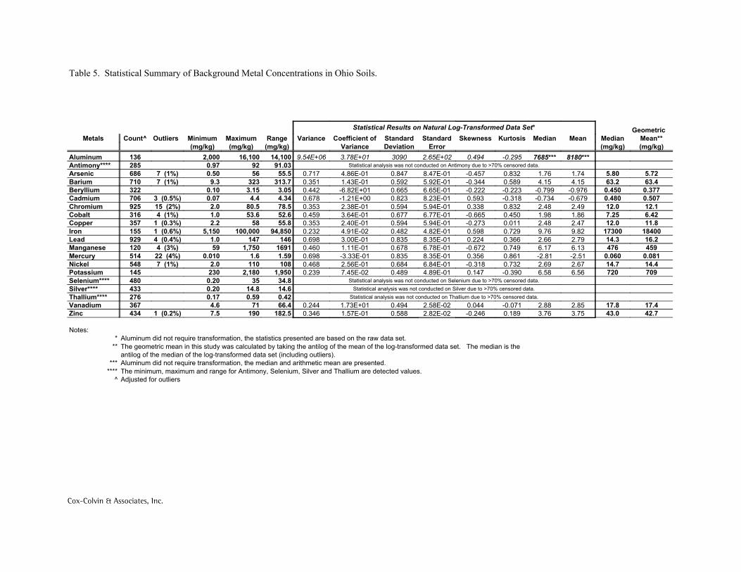
Table 5. Statistical Summary of Background Metal Concentrations in Ohio Soils.

GeometricStatistical Results on Natural Log-Transformed Data Set*Mean**MedianMeanMedianKurtosisSkewnessStandardStandardCoefficient ofVarianceRangeMaximumMinimumOutliersCount^Metals(mg/kg)(mg/kg)ErrorDeviationVariance(mg/kg)(mg/kg)(mg/kg)

8180***7685***-0.2950.4942.65E+0230903.78E+019.54E+0614,10016,1002,000136AluminumStatistical analysis was not conducted on Antimony due to >70% censored data.91.03920.97285Antimony****

5.725.801.741.760.832-0.4578.47E-010.8474.86E-010.71755.5560.507 (1%)686Arsenic63.463.24.154.150.589-0.3445.92E-010.5921.43E-010.351313.73239.37 (1%)710Barium

0.3770.450-0.976-0.799-0.223-0.2226.65E-010.665-6.82E+010.4423.053.150.10322Beryllium0.5070.480-0.679-0.734-0.3180.5938.23E-010.823-1.21E+000.6784.344.40.073 (0.5%)706Cadmium12.112.02.492.480.8320.3385.94E-010.5942.38E-010.35378.580.52.015 (2%)925Chromium6.427.251.861.980.450-0.6656.77E-010.6773.64E-010.45952.653.61.04 (1%)316Cobalt11.812.02.472.480.011-0.2735.94E-010.5942.40E-010.35355.8582.21 (0.3%)357Copper

18400173009.829.760.7290.5984.82E-010.4824.91E-020.23294,850100,0005,1501 (0.6%)155Iron16.214.32.792.660.3660.2248.35E-010.8353.00E-010.6981461471.04 (0.4%)929Lead4594766.136.170.749-0.6726.78E-010.6781.11E-010.46016911,750594 (3%)120Manganese

0.0810.060-2.51-2.810.8610.3568.35E-010.835-3.33E-010.6981.591.60.01022 (4%)514Mercury14.414.72.672.690.732-0.3186.84E-010.6842.56E-010.4681081102.07 (1%)548Nickel7097206.566.58-0.3900.1474.89E-010.4897.45E-020.2391,9502,180230145Potassium

Statistical analysis was not conducted on Selenium due to >70% censored data.34.8350.20480Selenium****Statistical analysis was not conducted on Silver due to >70% censored data.14.614.80.20433Silver****

Statistical analysis was not conducted on Thallium due to >70% censored data.0.420.590.17276Thallium****17.417.82.852.88-0.0710.0442.58E-020.4941.73E+010.24466.4714.6367Vanadium42.743.03.753.760.189-0.2462.82E-020.5881.57E-010.346182.51907.51 (0.2%)434Zinc

Notes:Aluminum did not require transformation, the statistics presented are based on the raw data set.*The geometric mean in this study was calculated by taking the antilog of the mean of the log-transformed data set. The median is the **antilog of the median of the log-transformed data set (including outliers).Aluminum did not require transformation, the median and arithmetic mean are presented. ***The minimum, maximum and range for Antimony, Selenium, Silver and Thallium are detected values.****Adjusted for outliers^


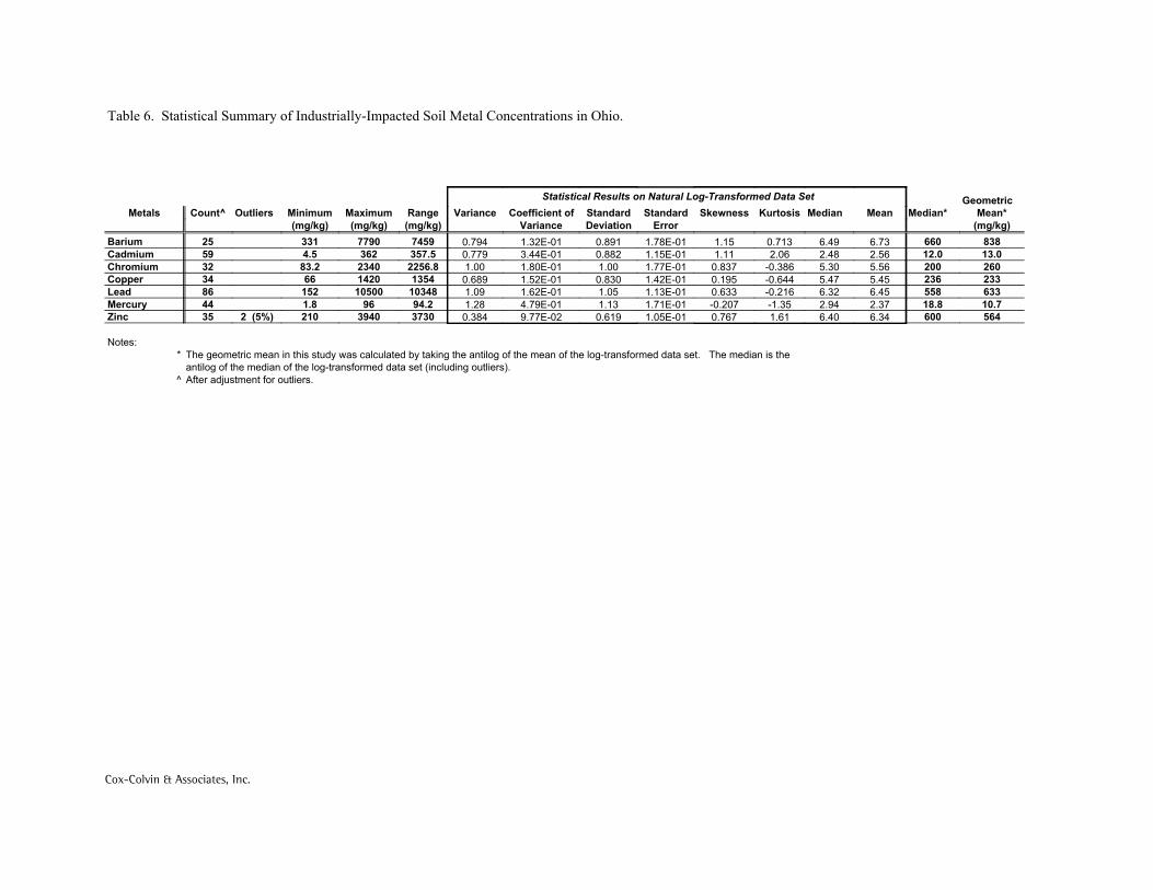
Table 6. Statistical Summary of Industrially-Impacted Soil Metal Concentrations in Ohio.

GeometricStatistical Results on Natural Log-Transformed Data SetMean*Median*MeanMedianKurtosisSkewnessStandardStandardCoefficient ofVarianceRangeMaximumMinimumOutliersCount^Metals

(mg/kg)ErrorDeviationVariance(mg/kg)(mg/kg)(mg/kg)8386606.736.490.7131.151.78E-010.8911.32E-010.7947459779033125Barium13.012.02.562.482.061.111.15E-010.8823.44E-010.779357.53624.559Cadmium2602005.565.30-0.3860.8371.77E-011.001.80E-011.002256.8234083.232Chromium2332365.455.47-0.6440.1951.42E-010.8301.52E-010.689135414206634Copper6335586.456.32-0.2160.6331.13E-011.051.62E-011.09103481050015286Lead10.718.82.372.94-1.35-0.2071.71E-011.134.79E-011.2894.2961.844Mercury5646006.346.401.610.7671.05E-010.6199.77E-020.384373039402102 (5%)35Zinc

Notes:The geometric mean in this study was calculated by taking the antilog of the mean of the log-transformed data set. The median is the *antilog of the median of the log-transformed data set (including outliers).After adjustment for outliers.^


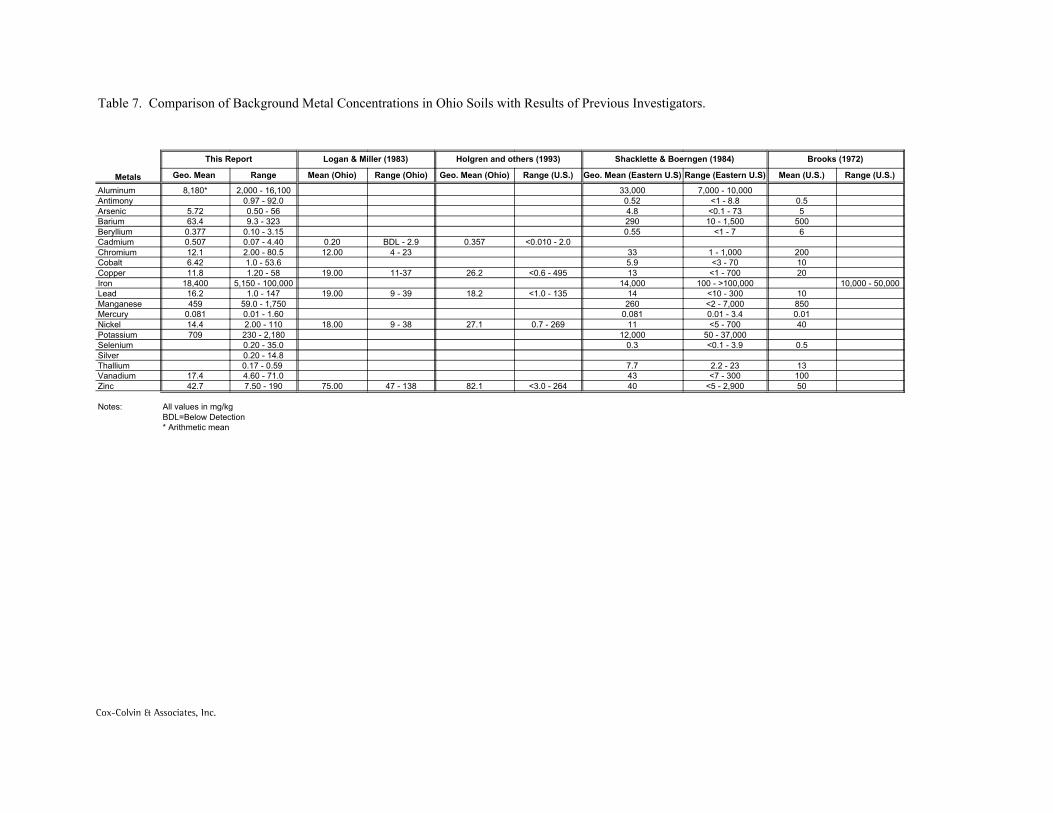
Table 7. Comparison of Background Metal Concentrations in Ohio Soils with Results of Previous Investigators.

Brooks (1972)Shacklette & Boerngen (1984)Holgren and others (1993)Logan & Miller (1983)This Report

Range (U.S.)Mean (U.S.)Range (Eastern U.S)Geo. Mean (Eastern U.S)Range (U.S.)Geo. Mean (Ohio)Range (Ohio)Mean (Ohio)RangeGeo. Mean Metals7,000 - 10,00033,0002,000 - 16,1008,180*Aluminum

0.5<1 - 8.80.520.97 - 92.0Antimony5<0.1 - 734.80.50 - 565.72Arsenic

50010 - 1,5002909.3 - 32363.4Barium6<1 - 70.550.10 - 3.150.377Beryllium

<0.010 - 2.00.357BDL - 2.90.200.07 - 4.400.507Cadmium2001 - 1,000334 - 2312.002.00 - 80.512.1Chromium10<3 - 705.91.0 - 53.66.42Cobalt20<1 - 70013<0.6 - 49526.211-3719.001.20 - 5811.8Copper

10,000 - 50,000100 - >100,00014,0005,150 - 100,00018,400Iron10<10 - 30014<1.0 - 13518.29 - 3919.001.0 - 14716.2Lead850<2 - 7,00026059.0 - 1,750459Manganese0.010.01 - 3.40.0810.01 - 1.600.081Mercury40<5 - 700110.7 - 26927.19 - 3818.002.00 - 11014.4Nickel

50 - 37,00012,000230 - 2,180709Potassium0.5<0.1 - 3.90.30.20 - 35.0Selenium

0.20 - 14.8Silver132.2 - 237.70.17 - 0.59 Thallium100<7 - 300434.60 - 71.017.4Vanadium50<5 - 2,90040<3.0 - 26482.147 - 13875.007.50 - 19042.7Zinc

All values in mg/kgNotes:BDL=Below Detection* Arithmetic mean


Logan and Miller, 1983

Defiance Henry

PauldingPutnam Hancock

HardinAllen

Van Wert

Mercer

Butler

Preble

Clark

Champaign

Logan

Marion

Darke

Shelby

Miami

Warren

Greene

Madison

Union Delaware

Morrow

Knox

Holmes

Wayne Stark

Clinton

FayettePickaway

Franklin

Licking

Coshocton

HighlandHamilton

BrownAdams Scioto

PikeJackson

Lawrence

Galia

Meigs

Ross

Hocking

Farifield Perry

Muskingum

Guernsey

VintonAthens

Morgan

Washington

Noble Monroe

Belmont

Harrison

Columbiana

Carroll

Auglaize

Ottawa

Sandusky

Seneca

Crawford

Huron

Erie

Wyandot

Richland

MedinaSummit

Portage

Mahoning

Trumbull

Ashtabula

Geauga

Lake

Lorain

Cuyahoga

Wood

LucasFulton

Williams

Cox and Colvin, 1996

Defiance Henry

PauldingPutnam Hancock

HardinAllen

Van Wert

Mercer

Butler

Preble

Clark

Champaign

Logan

Marion

Darke

Shelby

Miami

Warren

Greene

Madison

Union Delaware

Morrow

Knox

Holmes

Wayne Stark

Clinton

FayettePickaway

Franklin

Licking

Coshocton

HighlandHamilton

BrownAdams Scioto

PikeJackson

Lawrence

Galia

Meigs

Ross

Hocking

Farifield Perry

Muskingum

Guernsey

VintonAthens

Morgan

Washington

Noble Monroe

Belmont

Harrison

Columbiana

Carroll

Auglaize

Ottawa

Sandusky

Seneca

Crawford

Huron

Erie

Wyandot

Richland

MedinaSummit

Portage

Mahoning

Trumbull

Ashtabula

Geauga

Lake

Lorain

Cuyahoga

Wood

LucasFulton

Williams


Figure 2b. Probability Plot of the Two Population Data Setin Figure 2a.

Figure 2a. Frequency Diagram of a Data Set with TwoPopulations.

Frequency Diagram

Freq

uenc

y

0

20

40

60

80

100

120

0 1 2 3 4 5 6 7 8 9 10 11

Probability Plot

Probability 0

2

4

6

8

10

.9999 .999 .99 .9 .5 .1 .01 .001 .0001

Population A

Population A

Population B

Threshold orInflection Point

Probability Plot

Frequency Plot

Concentration

Probability Plot for Zinc

Probability

Nat

ural

Log

of C

once

ntra

tion

(mg/

kg)

0

2

4

6

8

10

.9999 .999 .99 .9 .5 .1 .01 .001 .0001

Figure 2c. Frequency Diagram of the Zinc DataSet.

Figure 2d. Probability Plot of the Zinc Data Set inFigure 2c.

Frequency Plot for Zinc

Natural Log of Concentration (mg/kg)

Freq

uenc

y

0

20

40

60

80

100

120

-2 0 2 4 6 8 10 12

Population A

Population B

Population B

Population AThreshold or

Inflection Point

Population B


Figure 2b. Probability Plot of the Two Population Data Setin Figure 2a.

Figure 2a. Frequency Diagram of a Data Set with TwoPopulations.

Frequency Diagram

Freq

uenc

y

0

20

40

60

80

100

120

0 1 2 3 4 5 6 7 8 9 10 11

Probability Plot

Probability 0

2

4

6

8

10

.9999 .999 .99 .9 .5 .1 .01 .001 .0001

Population A

Population A

Population B

Threshold orInflection Point

Probability Plot

Frequency Plot

Concentration

Probability Plot for Zinc

Probability

Nat

ural

Log

of C

once

ntra

tion

(mg/

kg)

0

2

4

6

8

10

.9999 .999 .99 .9 .5 .1 .01 .001 .0001

Figure 2c. Frequency Diagram of the Zinc DataSet.

Figure 2d. Probability Plot of the Zinc Data Set inFigure 2c.

Frequency Plot for Zinc

Natural Log of Concentration (mg/kg)

Freq

uenc

y

0

20

40

60

80

100

120

-2 0 2 4 6 8 10 12

Population A

Population B

Population B

Population AThreshold or

Inflection Point

Population B


Aluminum

Probability

Con

cent

ratio

n (m

g/kg

)

0

2,000

4,000

6,000

8,000

10,000

12,000

14,000

16,000

18,000

.9999 .999 .99 .9 .5 .1 .01 .001 .0001

Plot of Raw Data

Figure 3. Probability Plots for Aluminum

Normality testing and statistical modeling of raw data

indicates that the data set is normally distributed witha single population.

Data PointsModeled Results

Statistical Summary

Single Background Population

Data Points = 136Minimum Value = 2,000 mg/kg

Maximum Value = 16,100 mg/kg

Mean = 8,180 mg/kg

Aluminum

Probability

Nat

ural

Log

of C

once

ntra

tion

(mg/

kg)

6

7

8

9

10

11

12

.9999 .999 .99 .9 .5 .1 .01 .001 .0001

Plot of Natural Log-Transformed Data

Cox-Colvin & Associates,Inc.

Adjusting for outliers improves the normality test

results as well as the visual match between the

statistical modeling results and the log-transformed

data.


indicates that the data set is not normally distributed.

Arsenic

Probability

Nat

ural

Log

of C

once

ntra

tion

(mg/

kg)

-10

-8

-6

-4

-2

0

2

4

6

8

10

.9999 .999 .99 .9 .5 .1 .01 .001 .0001

Arsenic

Probability

Con

cent

ratio

n (m

g/kg

)

-100

0

100

200

300

400

500

600

700

800

.9999 .999 .99 .9 .5 .1 .01 .001 .0001

Plot of Raw Data


Modeled Results Data Points

Figure 4. Probability Plots for Arsenic

Normality testing and statistical modeling of

log-transformed data indicates that the data set is

log-normally distributed with a single population.

Outlier testing indicates that the data set contains 7

outliers.

Statistical Summary


Data Points = 686*

Minimum Value = 0.5 mg/kg*

Maximum Value = 56 mg/kg*Geometric Mean = 5.72 mg/kg*

*After adjustment for outliers.

Outliers

Outliers

Arsenic (Adjusted for Outliers)

Probability

Nat

ural

Log

of C

once

ntra

tion

(mg/

kg)

-8

-6

-4

-2

0

2

4

6

8

.9999 .999 .99 .9 .5 .1 .01 .001 .0001

Cox-Colvin & Associates,I

Barium (Adjusted for Outliers)

Probability

Nat

ural

Log

of C

once

ntra

tion

(mg/

kg)

-6

-4

-2

0

2

4

6

8

10

.9999 .999 .99 .9 .5 .1 .01 .001 .0001




data.

Barium

Probability

Nat

ural

Log

of C

once

ntra

tion

(mg/

kg)

-6

-4

-2

0

2

4

6

8

10

.9999 .999 .99 .9 .5 .1 .01 .001 .0001

Barium

Probability

Con

cent

ratio

n (m

g/kg

)

-2,000

-1,000

0

1,000

2,000

3,000

4,000

5,000

6,000

7,000

8,000

.9999 .999 .99 .9 .5 .1 .01 .001 .0001

Plot of Raw Data


Figure 5. Probability Plots for Barium




Statistical Summary

Two Populations

Ln of Threshold Value = 5.8 Background Population

Data Points = 710*

Minimum Value = 9.3 mg/kg* Maximum Value = 323 mg/kg

Geometric Mean = 63.4 mg/kg*

Industrially-Impacted Soil Data Points = 25

Minimum Value = 331 mg/kg

Maximum Value = 7,790 mg/kg Geometric Mean = 838 mg/kg

Outliers

Threshold

Normality testing and statistical modeling oflog-transformed data indicates that the data set is

log-normally distributed with two populations. Outlier

testing indicates that the data set contains 7 outliers.

Cox-Colvin & Associates,

Beryllium

Probability

Nat

ural

Log

of C

once

ntra

tion

(mg/

kg)

-4

-3

-2

-1

0

1

2

3

4

.9999 .999 .99 .9 .5 .1 .01 .001 .0001

Beryllium

Probability

Con

cent

ratio

n (m

g/kg

)

-2

-1

0

1

2

3

4

5

.9999 .999 .99 .9 .5 .1 .01 .001 .0001

Plot of Raw Data


Figure 6. Probability Plots for Beryllium




Statistical Summary


Data Points = 322

Minimum Value = 0.1 mg/kg

Maximum Value = 3.15 mg/kg

Geometric Mean = 0.377 mg/kg




Outlier testing indicates that the data set contains nooutliers.


Cadmium (Adjusted for Outliers)

Probability

Nat

ural

Log

of C

once

ntra

tion

(mg/

kg)

-6

-4

-2

0

2

4

6

8

.9999 .999 .99 .9 .5 .1 .01 .001 .0001


results as well as the visual match between thestatistical modeling results and the log-transformed

data.


Plot of Raw Data

Cadmium

Probability

Nat

ural

Log

of C

once

ntra

tion

(mg/

kg)

-6

-4

-2

0

2

4

6

8

.9999 .999 .99 .9 .5 .1 .01 .001 .0001

Cadmium

Probability

Con

cent

ratio

n (m

g/kg

)

-100

0

100

200

300

400

500

.9999 .999 .99 .9 .5 .1 .01 .001 .0001

Figure 7. Probability Plots for Cadmium


Normality testing and statistical mormality testing

and staistical modeling of raw data indicates that thedata set is not normally distributed.

Statistical Summary

Threshold





Outliers

Two Populations Ln of Threshold Value = 1.5

Background Population

Data Points = 706* Minimum Value = 0.07 mg/kg*


Geometric Mean = 0.507 mg/kg* Industrially-Impacted Soil

Data Points = 59

Minimum Value = 4.5 mg/kg Maximum Value = 362 mg/kg



Chromium (Adjusted for Outliers)

Probability

Nat

ural

Log

of C

once

ntra

tion

(mg/

kg)

-6

-4

-2

0

2

4

6

8

.9999 .999 .99 .9 .5 .1 .01 .001 .0001



statistical modeling results and the log-transformeddata.

Figure 8. Probability Plots for Chromium

Plot of Raw Data


Chromium

Probability

Nat

ural

Log

of C

once

ntra

tion

(mg/

kg)

-6

-4

-2

0

2

4

6

8

10

.9999 .999 .99 .9 .5 .1 .01 .001 .0001

Chromium

Probability

Con

cent

ratio

n (m

g/kg

)

-500

0

500

1,000

1,500

2,000

2,500

.9999 .999 .99 .9 .5 .1 .01 .001 .0001


Modeling of raw data indicates that the data set is not

normally distributed.

Statistical SummaryThreshold

Outliers






Data Points = 32

Minimum Value = 83.2 mg/kg Maximum Value = 2,340 mg/kg

Geometric Mean = 260 mg/kg



log-normally distributed with two populations. Outli

testing indicates that the data set contains 15 outliers





data.

Cobalt

Probability

Nat

ural

Log

of C

once

ntra

tion

(mg/

kg)

-2

-1

0

1

2

3

4

5

.9999 .999 .99 .9 .5 .1 .01 .001 .0001

Cobalt

Probability

Con

cent

ratio

n (m

g/kg

)

-10

0

10

20

30

40

50

60

70

.9999 .999 .99 .9 .5 .1 .01 .001 .0001

Plot of Raw Data

Figure 9. Probability Plots for Cobalt

Normality testing and statistical mdeling of raw data




Statistical Summary


Data Points = 316*




* After adjustment for outliers.





outliers.

Cobalt (Adjusted for Outliers)

Probability

Nat

ural

Log

of C

once

ntra

tion

(mg/

kg)

-2

-1

0

1

2

3

4

5

.9999 .999 .99 .9 .5 .1 .01 .001 .0001

Outliers


Copper (Adjusted for Outliers)

Probability

Nat

ural

Log

of C

once

ntra

tion

(mg/

kg)

0

2

4

6

8

10

.9999 .999 .99 .9 .5 .1 .01 .001 .0001




data.


Plot of Raw DataCopper

Probability

Con

cent

ratio

n (m

g/kg

)

-400

-200

0

200

400

600

800

1,000

1,200

1,400

1,600

.9999 .999 .99 .9 .5 .1 .01 .001 .0001

Copper

Probability

Nat

ural

Log

of C

once

ntra

tion

(mg/

kg)

0

2

4

6

8

10

.9999 .999 .99 .9 .5 .1 .01 .001 .0001

Figure 10. Probability Plots for Copper




Statistical Summary

Threshold




Maximum Value = 58 mg/kg


Data Points = 34

Minimum Value = 66 mg/kg Maximum Value = 1,420 mg/kg





testing indicates that the data set contains 1 outlier.

Outlier





data.

Figure 11. Probability Plots for Iron

Iron

Probability

Nat

ural

Log

of C

once

ntra

tion

(mg/

kg)

2

4

6

8

10

12

.9999 .999 .99 .9 .5 .1 .01 .001 .0001

Iron

Probability

Con

cent

ratio

n (m

g/kg

)

-20,000

0

20,000

40,000

60,000

80,000

100,000

.9999 .999 .99 .9 .5 .1 .01 .001 .0001

Plot of Raw Data

Iron (Adjusted for Outliers)

Probability

Nat

ural

Log

of C

once

ntra

tion

(mg/

kg)

2

4

6

8

10

12

.9999 .999 .99 .9 .5 .1 .01 .001 .0001

Normality testing and statistical modeling of raw dataindicates that the data set is not normally distributed.



Statistical Summary


Data Points = 155*

Minimum Value = 5,150 mg/kg*


Geometric Mean = 18,400 mg/kg*


Outlier


log-transformed data indicates that the data set islog-normally distributed with two populations. Outlier

testing indicates that the data set contains 1 outlier.


Lead (Adjusted for Outliers)

Probability

Nat

ural

Log

of C

once

ntra

tion

(mg/

kg)

-4

-2

0

2

4

6

8

10

.9999 .999 .99 .9 .5 .1 .01 .001 .0001

Adjusting for outliers improves the normality testresults as well as the visual match between the


data.

Plot of Raw Data


Lead

Probability

Nat

ural

Log

of C

once

ntra

tion

(mg/

kg)

-4

-2

0

2

4

6

8

10

.9999 .999 .99 .9 .5 .1 .01 .001 .0001

Lead

Probability

Con

cent

ratio

n (m

g/kg

)

-2,000

0

2,000

4,000

6,000

8,000

10,000

12,000

.9999 .999 .99 .9 .5 .1 .01 .001 .0001

Figure 12. Probability Plots for Lead


Normality testing and statistical modeling of raw dataindicates that the data set is not normally distributed.


Outliers

Two Populations

Ln of Threshold Value = 5.0

Background Population Data Points = 929*


Maximum Value = 147 mg/kg Geometric Mean = 16.2 mg/kg*

Industrially-Impacted Soil

Data Points = 86 Minimum Value = 152 mg/kg











data.

Manganese

Probability

Nat

ural

Log

of C

once

ntra

tion

(mg/

kg)

2

3

4

5

6

7

8

9

10

.9999 .999 .99 .9 .5 .1 .01 .001 .0001

Manganese

Probability

Con

cent

ratio

n (m

g/kg

)

-1,000

0

1,000

2,000

3,000

4,000

5,000

.9999 .999 .99 .9 .5 .1 .01 .001 .0001

Plot of Raw Data

Figure 13. Probability Plots for Manganese





Statistical Summary


Data Points = 120*

Minimum Value = 59 mg/kg*

Maximum Value = 1,750 mg/kg*

Geometric Mean = 459 mg/kg*


Manganese (Adjusted for Outliers)

Probability

Nat

ural

Log

of C

once

ntra

tion

(mg/

kg)

2

3

4

5

6

7

8

9

10

.9999 .999 .99 .9 .5 .1 .01 .001 .0001

Normality testing and statistical modeling oflog-transformed data indicates that the data set is



outliers.

Outliers

Outlier


Mercury (Adjusted for Outliers)

Probability

Nat

ural

Log

of C

once

ntra

tion

(mg/

kg)

-10

-8

-6

-4

-2

0

2

4

6

.9999 .999 .99 .9 .5 .1 .01 .001 .0001




data.


Plot of Raw Data

Mercury

Probability

Nat

ural

Log

of C

once

ntra

tion

(mg/

kg)

-10

-8

-6

-4

-2

0

2

4

6

.9999 .999 .99 .9 .5 .1 .01 .001 .0001

Mercury

Probability

Con

cent

ratio

n (m

g/kg

)

-20

0

20

40

60

80

100

.9999 .999 .99 .9 .5 .1 .01 .001 .0001

Figure 14. Probability Plots for Mercury










Data Points = 44

Minimum Value = 1.8 mg/kg Maximum Value = 96 mg/kg






Outliers




statistical modeling results and the log-transformeddata.

Nickel

Probability

Nat

ural

Log

of C

once

ntra

tion

(mg/

kg)

-2

0

2

4

6

8

.9999 .999 .99 .9 .5 .1 .01 .001 .0001

Nickel

Probability

Con

cent

ratio

n (m

g/kg

)

-500

0

500

1,000

1,500

2,000

.9999 .999 .99 .9 .5 .1 .01 .001 .0001

Plot of Raw Data

Figure 15. Probability Plots for Nickel





Statistical Summary

Single Background PopulationData Points = 548*


Maximum Value = 110 mg/kg*



Outliers

Outliers




Outlier testing indicates that the data set contains 7outliers.

Nickel (Adjusted for Outliers)

Probability

Nat

ural

Log

of C

once

ntra

tion

(mg/

kg)

-2

0

2

4

6

8

.9999 .999 .99 .9 .5 .1 .01 .001 .0001


Potassium

Probability

Nat

ural

Log

of C

once

ntra

tion

(mg/

kg)

4

5

6

7

8

9

10

.9999 .999 .99 .9 .5 .1 .01 .001 .0001

Potassium

Probability

Con

cent

ratio

n (m

g/kg

)

-500

0

500

1,000

1,500

2,000

2,500

.9999 .999 .99 .9 .5 .1 .01 .001 .0001

Plot of Raw Data

Figure 16. Probability Plots for Potassium





log-transformed data indicates that the data set islog-normally distributed with a single population.

Outlier testing indicates that there are no outliers.


Statistical Summary


Data Points = 145

Minimum Value = 230 mg/kgMaximum Value = 2,180 mg/kg



Vanadium

Probability

Nat

ural

Log

of C

once

ntra

tion

(mg/

kg)

0

.5

1

1.5

2

2.5

3

3.5

4

4.5

5

.9999 .999 .99 .9 .5 .1 .01 .001 .0001

Vanadium

Probability

Con

cent

ratio

n (m

g/kg

)

-20

0

20

40

60

80

100

.9999 .999 .99 .9 .5 .1 .01 .001 .0001

Plot of Raw Data

Figure 17. Probability Plots for Vanadium





log-transformed data indicates that the data set islog-normally distributed with a single population.

Outlier testing indicates that there are no outliers.


Statistical Summary


Data Points = 367

Minimum Value = 4.6 mg/kgMaximum Value = 71 mg/kg



Zinc (Adjusted for Outliers)

Probability

Nat

ural

Log

of C

once

ntra

tion

(mg/

kg)

0

2

4

6

8

10

.9999 .999 .99 .9 .5 .1 .01 .001 .0001




data.

Plot of Raw Data


Zinc

Probability

Nat

ural

Log

of C

once

ntra

tion

(mg/

kg)

0

2

4

6

8

10

.9999 .999 .99 .9 .5 .1 .01 .001 .0001

Zinc

Probability

Con

cent

ratio

n (m

g/kg

)

-5,000

0

5,000

10,000

15,000

20,000

.9999 .999 .99 .9 .5 .1 .01 .001 .0001

Figure 18. Probability Plots for Zinc




Statistical Summary

Threshold

Two Populations

Ln of Threshold Value = 5.3 Background Population

Data Points = 434*

Minimum Value = 7.5 mg/kg* Maximum Value = 190 mg/kg


Industrially-Impacted Soil Data Points = 35*

Minimum Value = 210 mg/kg

Maximum Value = 9,940 mg/kg* Geometric Mean = 564 mg/kg*

* After adjustment for outliers.

Normality testing and statistical mormality testing and

statistical modeling of log-transformed data indicates

that the data set is log-normally distributed with two

populations. Outlier testing indicates that the data setcontains 3 outliers.

Outliers

Outlier


Documents

Evaluation of Background Metal Concentrations in Ohio … · Evaluation of Background Metal Concentrations in Ohio Soils June 21, 1996 Cox-Colvin & Associates, Inc. 2 across the state,