Embed Size (px)
Citation preview

ESD-TR-88-232
Technical Report 822
Evaluation of Adaptive Phased Array Antenna Far Field Nulling Performance
in the Near Field Region
A.J. Fenn
19 January 1989
Lincoln Laboratory MASSACHUSETTS INSTITUTE OF TECHNOLOGY
LEXINGTON, MASSACHUSETTS
Prepared for the Department of the Air Force under Electronic Systems Division Contract F19628-85-C-0002.
Approved for public release; distribution unlimited.

The work reported in this document was performed at Lincoln Laboratory, a center for research operated by Massachusetts Institute of Technology, with the support of the Department of the Air Force under Contract F19628-85-C-0002.
This report may be reproduced to satisfy needs of U.S. Government agencies.
The views and conclusions contained in this document are those of the contractor and should not be interpreted as necessarily representing the official policies, either expressed or implied, of the United States Government.
The ESD Public Affairs Office has reviewed this report, and it is releasable to the National Technical Information Service, where it will be available to the general public, including foreign nationals.
This technical report has been reviewed and is approved for publication.
FOR THE COMMANDER
Hugh L. Southall, Lt. Col., USAF Chief, ESD Lincoln Laboratory Project Office
MASSACHUSETTS INSTITUTE OF TECHNOLOGY LINCOLN LABORATORY
EVALUATION OF ADAPTIVE PHASED ARRAY ANTENNA FAR FIELD NULLING PERFORMANCE
IN THE NEAR FIELD REGION
A.J. FENN Group 61
TECHNICAL REPORT 822
19 JANUARY 1989
Approved for public release; distribution unlimited.
LEXINGTON MASSACHUSETTS

ABSTRACT
A theory for analyzing the behavior of adaptive phased array antennas illuminated by a near field interference test source is presented. Conventional phased array near field focusing is used to produce an equivalent far field antenna pattern at a range distance of one to two aperture diameters from the adaptive antenna under test. The antenna is assumed to be a linear array of isotropic receive elements. The interferer is assumed to be a bandlimited noise source radiating from an isotropic antenna. The theory is developed for both partially and fully adaptive arrays. Results are presented for the fully adaptive array case with single and multiple interferers which indicate that near field and far field adaptive nulling can be equivalent. The adaptive nulling characteristics studied in detail are the array radiation patterns, adaptive cancellation, covariance matrix eigenvalues, and adaptive array weights.
in

TABLE OF CONTENTS
ABSTRACT iii
LIST OF ILLUSTRATIONS vii
1. INTRODUCTION 1
2. THEORY 7
2.1 General Adaptive Nulling Concepts 7
2.2 Near Field Formulation 9
2.3 Far Field Formulation 13
2.4 Near Field Boundary 14
3. RESULTS 17
3.1 Focused Linear Array Quiescent Conditions 17
3.2 Fully Adaptive Array Behavior 17
4. CONCLUSION 33
REFERENCES 34

LIST OF ILLUSTRATIONS
Figure No. Page
1-1 Geometry for Far Field and Near Field Interference: (a) Plane Wavefront and (b) Spherical Wavefront 2
1-2 Dispersion Multiplier as a Function of Interferer Incidence Angle for Various In- terferer Range Distances 4
2-1 Adaptive Beamfonaer Arrangements: (a) Fully Adaptive Array and (b) Partially Adaptive Array 8
2-2 Adaptive Phased Array Antenna Near Field Focusing Concept. A CW Radiat- ing Source Is Used to Illuminate the Array with a Calibration Signal and Phase Corrections Are Applied at the Array Weights to Focus the Antenna. The Array Then Forms a Main Beam in the Direction of the Focal Point and an Interference Source Is Placed on a Near Field Sidelobe. 10
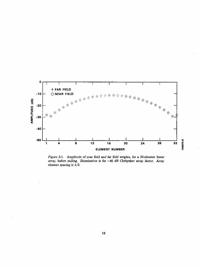
3-1 Amplitude of Near Field and Far Field Weights, for a 32-Element Linear Array, Before Nulling. Illumination Is for -40 dB Chebyshev Array Factor. Array Ele- ment Spacing Is A/2. 18
3-2 Focused 32-Element Linear Array Near Field/Far Field Radiation Patterns Before Nulling. Scan Angle Is 6 = 60° with —40 dB Chebyshev Illumination. Array El- ement Spacing is A/2. Dashed Curve Is for Near Field Focusing with Near Field Observation. Solid Curve Is for Far Field (r = oo) Focusing with Far Field Observation, (a) F/L = 1, (b) F/L = 1.5, and (c) F/L = 2. 19
3-3 Focused 32-Element Fully Adaptive Linear Array Near Field/ Far Field Radi- ation Patterns After Adaption. Nulling Bandwidth Is 1 MHz (Narrow Band Case). Interferer Is Located at 0 = 33°. Dashed Curve Is for Near Field Fo- cusing/ Observation/Interference. Solid Curve Is for Far Field (r = oo) Focus- ing/Observation/Interference, (a) F/L = 1, (b) F/L = 1.5, and (c) F/L = 2. 21
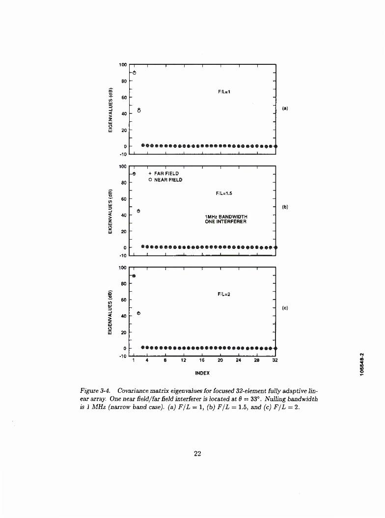
3-4 Covariance Matrix Eigenvalues for Focused 32-Element Fully Adaptive Linear Ar- ray. One Near Field/Far Field Interferer Is Located at 0 = 33°. Nulling Bandwidth Is 1 MHz (Narrow Band Case), (a) F/L = 1, (b) F/L = 1.5, and (c) F/L = 2. 22
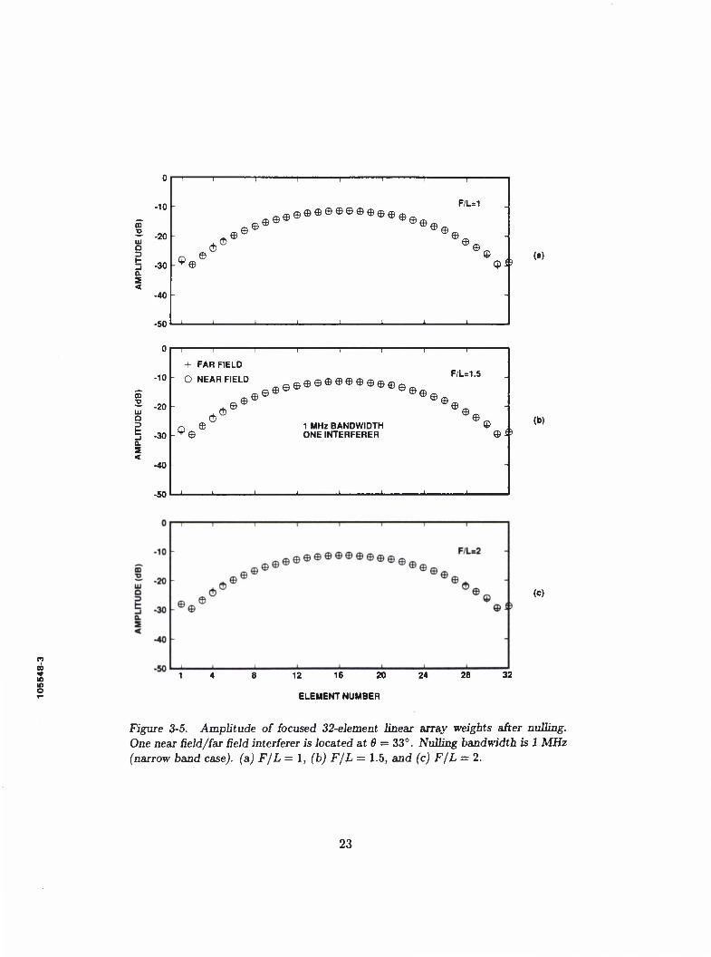
3-5 Amplitude of Focused 32-Element Linear Array Weights After Nulling. One Near Field/Far Field Interferer Is Located at 6 = 33°. Nulling Bandwidth Is 1 MHz (Narrow Band Case), (a) F/L = 1, (b) F/L = 1.5, and (c) F/L = 2. 23
vn

Figure No. Page
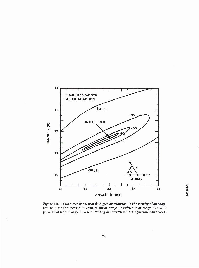
3-6 Two Dimensional Near Field Gain Distribution, in the Vicinity of an Adaptive Null, for the Focused 32-Element Linear Array. Interferer Is at Range F/L — 1 (n = 11.73 ft) and Angle 6t = 33°. Nulling Bandwidth Is 1 MHz (Narrow Band Case). 24
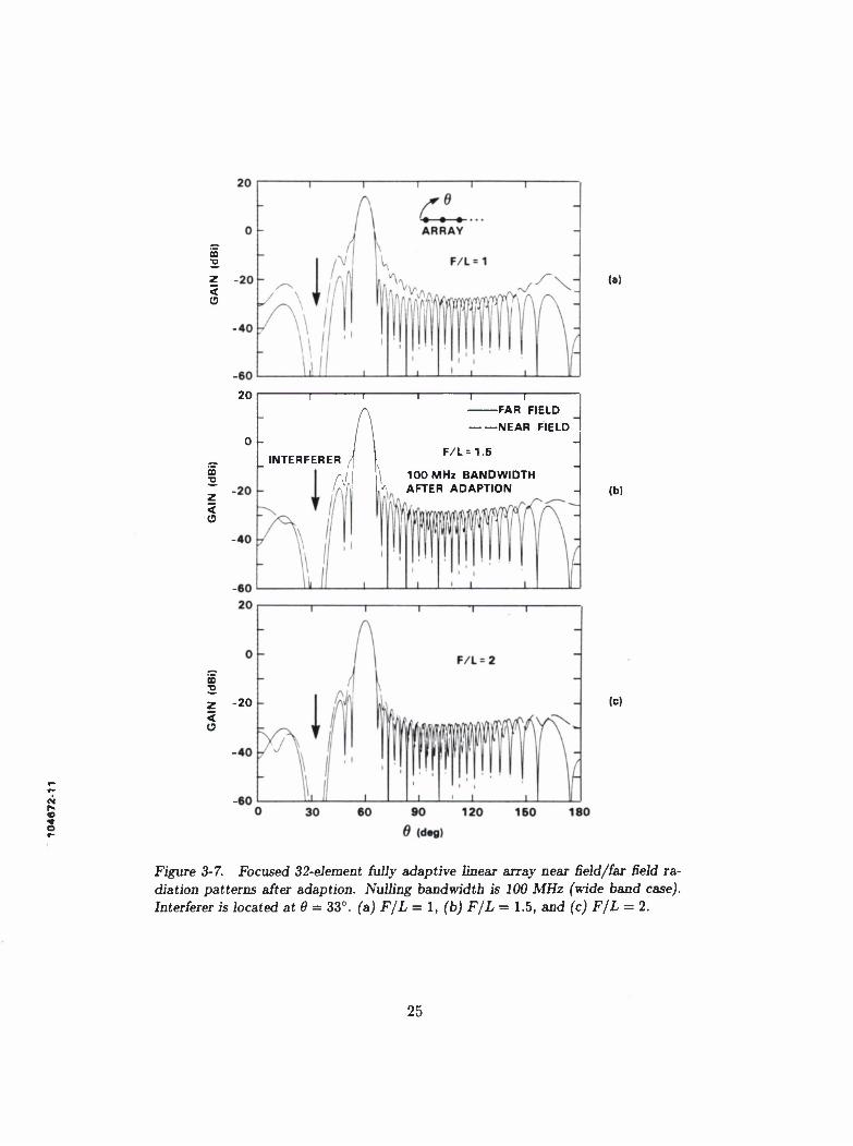
3-7 Focused 32-Element Fully Adaptive Linear Array Near Field/Far Field Radiation Patterns After Adaption. Nulling Bandwidth Is 100 MHz (Wide Band Case). Interferer Is Located at 9 = 33°. (a) F/L = 1, (b) FjL = 1.5, and (c) FjL = 2. 25
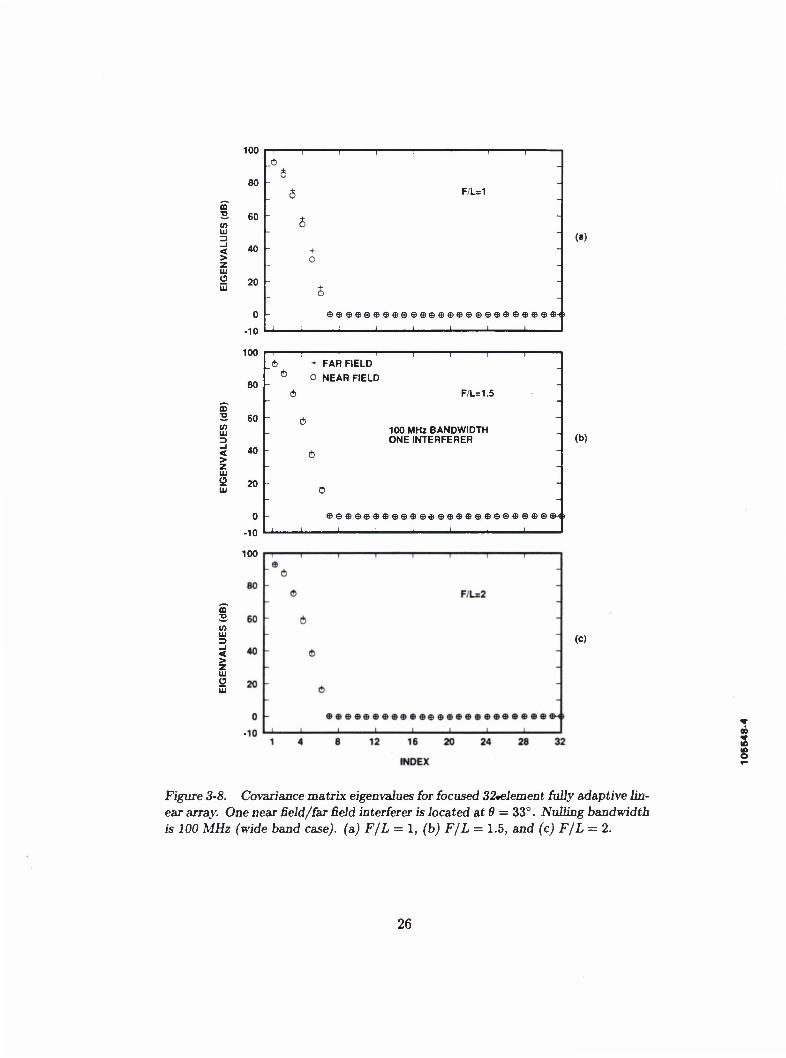
3-8 Covariance Matrix Eigenvalues for Focused 32-Element Fully Adaptive Linear Ar- ray. One Near Field/Far Field Interferer Is Located at 6 — 33°. Nulling Bandwidth 100 MHz (Wide Band Case), (a) F/L = 1, (b) F/L = 1.5, and (c) F/L = 2. 26
3-9 Amplitude of Focused 32-Element Linear Array Weights After Nulling. One Near Field/Far Field Interferer Is Located at 6 = 33°. Nulling Bandwidth Is 100 MHz Wide Band Case), (a) F/L = 1, (b) F/L = 1.5, and (c) F/L = 2. 27
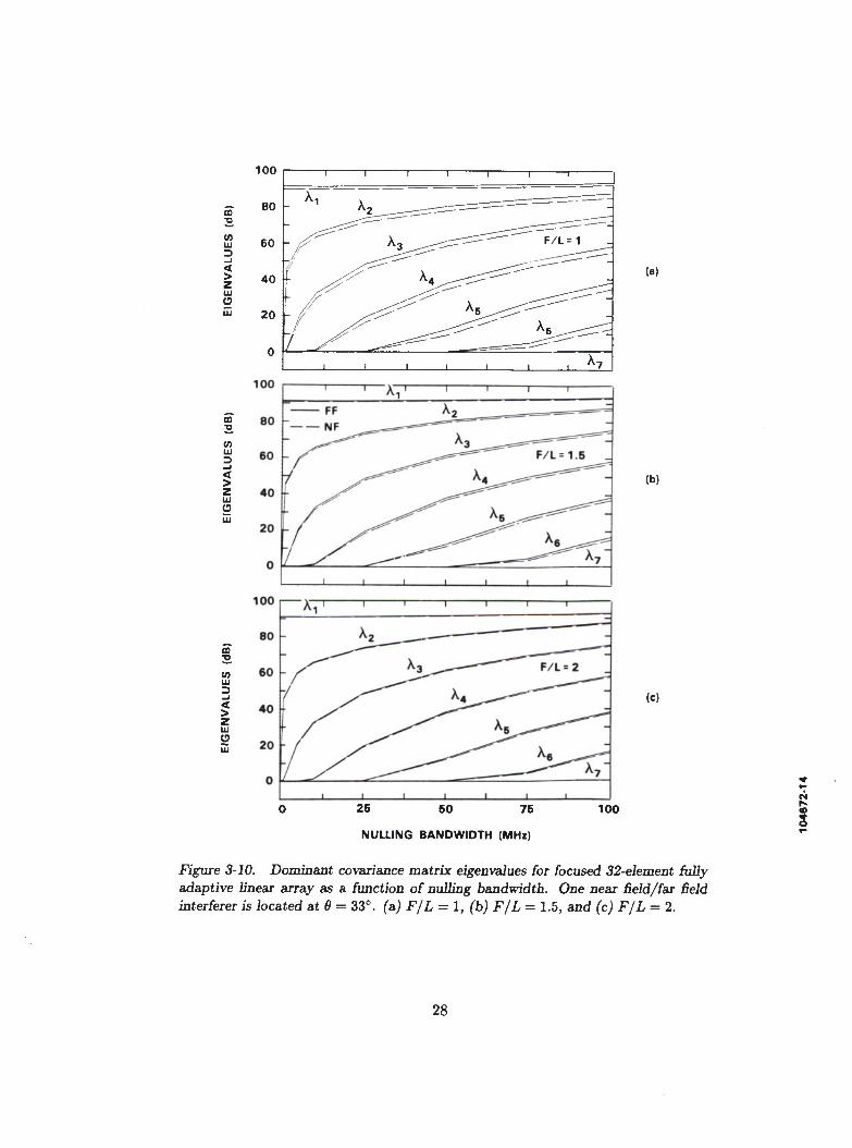
3-10 Dominant Covariance Matrix Eigenvalues for Focused 32-Element Fully Adaptive Linear Array as a Function of Nulling Bandwidth. One Near Field/Far Field Interferer Is Located at 6 = 33°. (a) F/L = 1, (b) F/L = 1.5, and (c) F/L = 2. 28
3-11 Focused 32-Element Fully Adaptive Linear Array Near Field/Far Field Radiation Patterns After Adaption. There Are 31 Interferers with Uniform Five-Degree Spacing (Excluding the Main Beam Region). Nulling Bandwidth Is 1 MHz. (a) F/L = 1, (b) F/L = 1.5, and (c) F/L = 2. 29
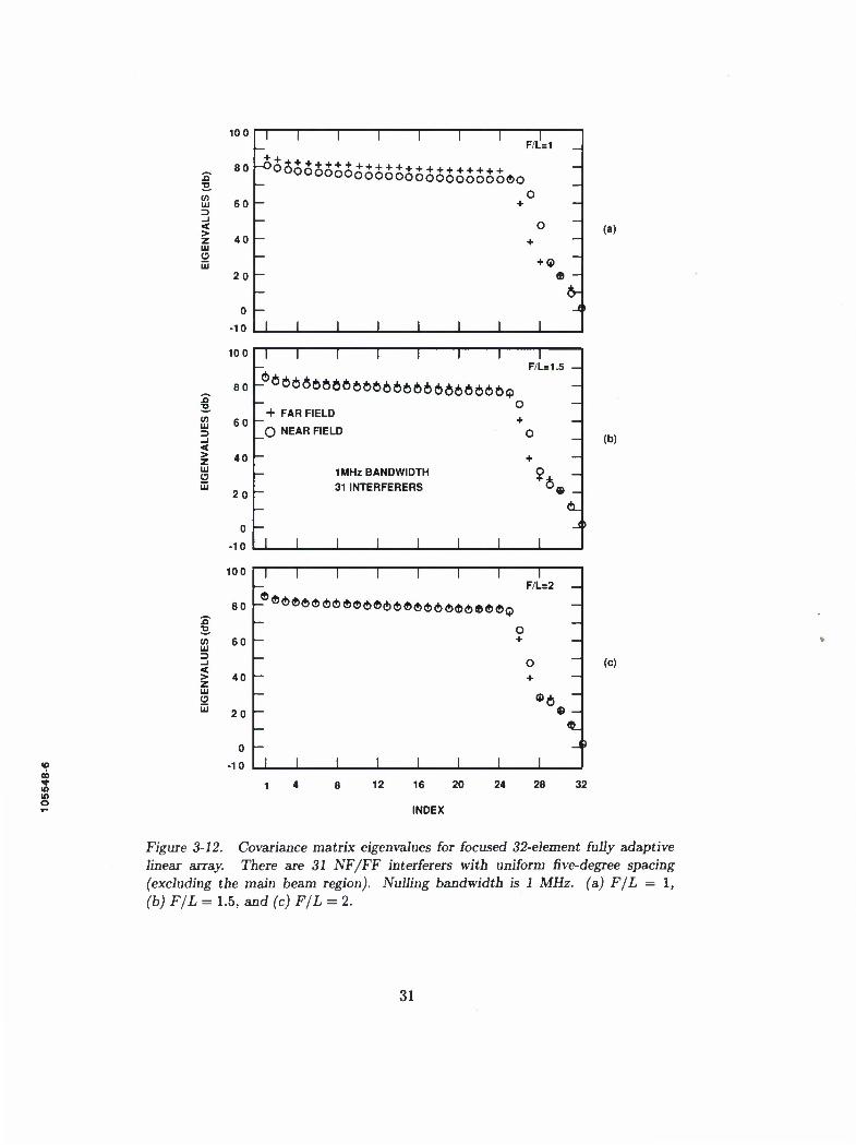
3-12 Covariance Matrix Eigenvalues for Focused 32-Element Fully Adaptive Linear Ar- ray. There Are 31 NF/FF Interferers with Uniform Five-Degree Spacing (Ex- cluding the Main Beam Region). Nulling Bandwidth Is 1 MHz. (a) F/L = 1, (b) F/L = 1.5, and (c) F/L = 2. 31
3-13 Amplitude of Focused 32-Element Fully Adaptive Linear Array Weights After Adaption. There Are 31 NF/FF Interferers with Uniform Five-Degree Spacing (Excluding the Main Beam Region). Nulling Bandwidth is 1 MHz. (a) F/L = 1, (b) F/L = 1.5, and (c) F/L = 2. 32
vm
1. INTRODUCTION
Electrically large phased array antennas having partially adaptive or fully adaptive nulling capability are often suggested for radar or communications applications. The adaptive nulling performance of these antennas is principally tested using conventional far field antenna ranges with far field (or plane wave) interferers. At microwave frequencies, this can lead to significant far field range distances which require that testing be made outdoors. For example, given a 20-m aperture at L-band, the usual far field range criterion R = 2D2/X yields a distance of approximately 3.5 km. Multiple, widely separated interferers make the far field range design more difficult. Near field testing, suitable for indoor measurements, is desirable as has been demonstrated in the case of near field scanning [1] for far field pattern determination and compact range reflector techniques [2] for far field radiation pattern and radar cross section determination.
Conventional near field scanning does not appear practical in the adaptive nulling antenna situation, as a mathematical transformation is usually required to determine the far field per- formance. Adaptive nulling requires a real-time interference wavefront. Furthermore, near field scanning reported in the literature is strictly single tone and is not compatible with adaptive nulling tests which often require the presence of a wide-bandwidth noise interferer (jammer). A compact range reflector is applicable to near field adaptive nulling as it generates a real-time wavefront. However, the compact range reflector does not easily lend itself to multiple widely- separated interferers. Thus, an alternate approach to adaptive array near field testing needs to be considered.
If the requirement for plane wave test conditions is relaxed and spherical wave incidence is allowed, as will be shown, for a focused phased array antenna, near field testing with a fixed isotropic interferer is possible. It is shown, by example, that at one to two aperture diameters range, J near field interferers (where J is a number typically less than the number of adaptive array channels) can be equivalent to J far field interferers. The contrast between plane wave incidence and spherical wave incidence is depicted in Figure 1-1. The amount of wavefront dispersion observed by the linear array is a function of the bandwidth, array length, and angle of incidence. Interference wavefront dispersion is an effect which can limit the depth of null (or cancellation) achieved by an adaptive antenna[3].
A basic dispersion model for spherical wave incidence and plane wave incidence can be made by considering only the wavefront dispersion observed by the end points of an adaptive array. This calculation is useful in gaining some initial insight into how near field (NF) nulling will relate to far field (FF) nulling. Consider first, a plane wave arriving from infinity and an array of length L as shown in Figure 1-1 (a). The dispersion for this case is denoted IFF and is computed according to the product of bandwidth and time delay as
T3T
IFF = PFF (1-1) C
where B is the nulling bandwidth and c is the speed of fight. In Equation (1.1) the quantity f}pp will be referred to as the far field dispersion multiplier, which is simply given by

PLANE WAVEFRONT
LINEAR ARRAY
r\ = Vr? + Lrjcos d, + -
rjg = \Af - LriCos 6X + -
SPHERICAL POINT SOURCE WAVEFRONT
(b)
LINEAR ARRAY
Figure 1-1. Geometry for far Geld and near field interference: (a) plane wavefront and (b) spherical wavefront.

0FF= COS di (1.2)
where 6{ is the angle of incidence with respect to the axis of the array. Note that the dispersion is maximum for endfire incidence (6t — 0) and is zero for broadside incidence (&i = 7r/2). Next, consider the same array and now a point source, at range r = T{ and angle 0 = 6(, which produces a spherical wavefront as depicted in Figure l-l(b). The near field dispersion, denoted JNF, is given by
ID T
7NF = —PNF (1.3) C
where the quantity /3^p denotes the near field dispersion multiplier which, from the difference between the path lengths r\ and r*N, is expressed as
PNF = \/a2 + acos#, + - - Ja2 - a cos 6i + - (1.4)
where
«=f (1.5)
and where F is the focal length of the array such that r, = F. In comparing Equations (1.1) and (1.3), the far field and near field dispersions differ only by their respective dispersion multipliers 0FF and &NF- If near field nulling is equivalent to far field nulling then Equation (1.2) must be equal to Equation (1.4). Figure 1-2 shows a plot of .0FF and 0NF vs angle of incidence for values of a=0.2 to 2 (that is, focal lengths 0.2L to 2L). From this figure it is seen that the near field dispersion approaches the value of the far field dispersion for source range distances greater than approximately one aperture diameter (a > 1). Clearly, at source range distances such that a < 0.5 (one-half aperture diameter) the near field dispersion is significantly different than the far field dispersion. Thus, for this simple dispersion model it is expected that near field adaptive nulling will be similar to far field nulling at source range distances greater than one aperture diameter.
A more precise dispersion model is essentially the characteristics of the interference covariance matrix—namely its eigenvalues or degrees of freedom [3,4]. The covariance matrix contains all wavefront dispersion presented to the adaptive channels, not just the contributions from the array edge as modeled above. The interference covariance matrix eigenvalues can be used to quantify and to compare the dispersion present for plane wave and spherical wave incidence. For near field adaptive nulling to be equivalent to far field adaptive nulling, it is assumed that the NF/FF interference covariance matrix eigenvalues must be equivalent. Additionally, it is assumed that the NF/FF adaptive array weights, cancellation of interference power, and radiation patterns must also be equivalent.
An example of near field adaptive nulling has been given by Hudson [5]. A two-element array with a single near field CW (continuous wave) interferer was investigated. It was shown that

0.8
en UJ
§j 0.6 D s z g w B UJ
8>04
oa.
0.2
K^^ 1 1 1 I I ' ' SOURCE
\ \
V _
N. N^^ 2.0
oo A —
|__L^|
>v 0.5>v \
""-»»w 04 \ >v ^mm
" -"^ O-^Nw
-
0.25^^ ^N
-
a = F/L
-
^^ L IS THE ARRAY LENGTH ^~"
-
F IS THE FOCAL DISTANCE
I I I I ' I
k -
30 0, (deg)
60 90
Figure 1-2. Dispersion multiplier as a function of interferer incidence angle for various interferer range distances.
a null could be formed at a near field point. However, no attempt to determine if there is any similarity between near field and far field nulling was made.
Investigations of NF/FF adaptive nulling for linear arrays of isotropic receive elements have been performed [6,7]. Near field adaptive nulling results for a single interferer at a range of 1.7L for sidelobe canceller [6] and fully adaptive [7] arrays have been presented. The effects of nulling bandwidth were taken into account. Comparisons with far field adaptive nulling indicated an excellent NF/FF equivalence. A detailed analysis of near field adaptive nulling in the range of one to two aperture diameters has been given for a sidelobe canceller [8]. The purpose of the present report is to investigate the corresponding behavior of a fully adaptive array.
This report is organized such that, a theory for analyzing and comparing both near field and far field adaptive nulling is presented in Section II. General adaptive nulling concepts are addressed first. Near field focusing and the near field nulling concept are then described. The theory is developed for the situation of a linear array of isotropic receive elements and isotropically radiating interference sources. Equations for the NF/FF covariance matrices and radiation patterns of fully adaptive and sidelobe canceller adaptive arrays are given. A discussion of the boundaries of the near, Fresnel, and far zones is included. The emphasis of this report is on near field nulling although the theory is equally valid in the Fresnel zone. In Section III, results are presented which show that, at one to two aperture diameters range, a fully adaptive array responds in the same manner to near field sources as it does to far field sources. Application of this near field technique to testing main beam clutter cancellation is documented [9].
2. THEORY
2.1 GENERAL ADAPTIVE NULLING CONCEPTS
Consider an N-element linear array of isotropic point receiving antennas. Let an interference wavefront be impressed across the array, which results in a set of induced terminal voltages denoted as v\,V2, • • • , u/v7- As shown in Figure 2-1, two types of arrays will be considered—fully adaptive arrays and sidelobe canceller arrays. The number of adaptive channels is denoted as M. For the fully adaptive array M = N, and for the sidelobe canceller M = 1 + Naux where Naux is the number of auxiliary channels. In this report, ideal weights are assumed with w = (w\,W2, • • • ,WM)
T denoting the adaptive channel weight vector and W = (W\, W2, • • •, WN)
T
denoting the sidelobe canceller array element weight vector, as shown in Figure 2-1 (superscript T means transpose). The fundamental quantities required in fully characterizing the incident field, for adaptive nulling purposes, are the adaptive channel cross correlations.
The cross correlation Rmn of the received voltages in the mth and nth adaptive channels is given by
Rmn = E(vmVn) (2.1)
where * means complex conjugate and E(-) means mathematical expectation. Since vm and vn
represent voltages of the same waveform, but at different times, Rmn is also referred to as an autocorrelation function .
In the frequency domain, assuming the interference has a bandlimited white noise power spec- tral density, Equation (2.1) can be expressed as the frequency average
Rmn = ^Jf2Vm(fK(f)df (2.2)
where B = /2 — /1 is the nulling bandwidth and fc is the center frequency. It should be noted that vm(f) takes into account the wavefront shape which can be spherical or planar.
Let the channel or interference covariance matrix be denoted by R . If there are J uncorrelated broadband interference sources, then the ./-source covariance matrix is the sum of the covariance matrices for the individual sources, that is,
J
R = Y,Ri + I (2.3)
where Ri is the covariance matrix of the ith source, / is the identity matrix which is used to represent the thermal noise level of the receiver.
Prior to generating an adaptive null, the adaptive channel weight vector, w, is chosen to synthesize a desired quiescent radiation pattern. When interference is present, the optimum set of weights, denoted wa, to form an adaptive null is computed by [10]

ARRAY
i) ^•••Sj»"N
INTERFERER
"1 ADAPTIVE CONTROL
I ADAPTIVE 1
BEAMFORMER
OUTPUT
(a)
ARRAY w w w w
JS INTERFERER
AUXILIARIES
N N--S...H
MAIN 6
n. ADAPTIVE jr-L-i CONTROL jU
ri w^.4wm|..|W(vj |
i i
"ADAPTIVE [BEAMFORMER j
OUTPUT
(b) §
Figure 2-1. Adaptive beamformer arrangements: (a) fully adaptive array and (b) partially adaptive array.

wa = BTl • wq (2.4)
where _1 means inverse and wq is the quiescent weight vector.
The output power at the adaptive array summing junction is given by
p = wjRw (2.5)
where t means complex conjugate transpose. The interference-plus-noise to noise ratio, denoted INR, is computed as the ratio of the output power (defined in Equation (2.5)) with the interferer present to the output power with only receiver noise present, that is,
w^ • R • w INR= . . (2.6)
The adaptive array cancellation ratio, denoted C, is defined here as the ratio of interference output power after adaption to the interference output power before adaption, that is,
C = ^. (2.7) Pq
Substituting Equation (2.5) in Equation (2.7) yields
C=W*\'*mW\ (2.8)
Next, the covariance matrix defined by the elements in Equation (2.2) is Hermitian (that is, R = R*) which, by the spectral theorem, can be decomposed in eigenspace as [11]
M
R=y£xkekel (2.9) fc=i
where A*,A: = 1,2,•• •, M are the eigenvalues of R, and ek,k = 1,2,•• •, M are the associated eigenvectors of R. The covariance matrix eigenvalues (Ai, A2, • ••, AM) are a convenient quantita- tive measure of the utilization of the adaptive array degrees of freedom.
2.2 NEAR FIELD FORMULATION
2.2.1 Focused Near Field Nulling Concept
To properly utilize the near field nulling technique described here, it is assumed that the quiescent near field radiation pattern of the array should have the same characteristics as the quiescent far field radiation pattern of the array. This means typically that a main beam and side lobes should be formed. To produce an array near field pattern which is approximately equal to the far field pattern, phase focusing can be used [12]. Consider Figure 2-2 which shows a
9

ARRAY OUTPUT
--»N CW CALIBRATION SOURCE AT FOCUS
INTERFERER (ri# 0,)
ON NEAR-FIELD SIDE LOBE
L=ARRAY LENGTH
fj = INTERFERER RANGE (Ls£rjSg2L)
ID
ID
s 10 o
Figure 2-2. Adaptive phased array antenna near field focusing concept. A CW radiating source is used to illuminate the array with a calibration signal and phase corrections are applied at the array weights to focus the antenna. The array then forms a main beam in the direction of the focal point and an interference source is placed on a near fieid sidelobe.
10
CW calibration source located at a desired focal point of the array. The array can maximize the signal received from the calibration source by adjusting its phase shifters such that the spherical wavefront phase variation is removed. One way to do this is to choose a reference path length as the distance from the focal point to the center of the array. This distance is denoted rp, and the distance from the focal point to the nth array element is denoted r£. The voltage received at the nth array element is expressed as
eJ2*(rF-r£)/\c VF
n = ~ ~F (2-10)
where Ac is the wavelength at center frequency fc. To maximize the received voltage at the array output, it is necessary to add ^n radians to the nth element, that is,
*n = 27r(r£ - rF)/\c. (2.11)
The resulting radiation pattern at range rF looks much like an ordinary far field pattern. A main beam will be pointed at the array focal point. Side lobes will exist at angles away from the main beam. An interferer can then be placed on a near field side lobe, at range r< = r?, as depicted in Figure 2-2.
2.2.2 Covariance Matrix
The near field covariance matrix elements are derived in the following manner [8]: Refer to Figure l-l(b) which shows the near field geometry under consideration. An interference source, whose power spectral density is assumed to be bandlimited white noise, is represented by the index i in a set of J sources. Let it be assumed that the power received at the center element of the array from the ith source, denoted Pi, is measured relative to thermal noise. The voltage received by the nth array element is then given by
-j2*/ri,/c < = JP~- j (2.12)
where rj, is the distance between the nth array element and the interferer. Substituting Equation (2.12) in Equation (2.2) and integrating, gives the correlation between either two channels in a fully adaptive array or two auxiliary channels in a sidelobe canceller array, as
R• = Pi4-e-^^^Tmn) (2.13) rmTn 7r-DTmn
where rj is the range from the array center to the interferer and
Tmn = (rin-ri
n)/c (2.14)
11

is the interferer time differential factor between elements m and n. In Equation (2.13), rf has been included as a convenient normalization factor.
Next, for a sidelobe canceller array, the main channel received voltage is expressed as
JL e-j27r/rj,/c vmain = V5£wA—ji—• (2-15)
m=l m
Substituting Equations (2.12) and (2.15) in Equation (2.2) and integrating yields the cross cor- relation between the main channel and the nth auxiliary channel
flmain,aux„ = P'r« Z. ^m-jj THZ • (2-16) m=l 'm'n njJ>mn
The main channel cross correlation is found using Equation (2.15) in Equation (2.2) as
•"maintain _-^'^ 2^ 2^ ^m^n t { R (l.M) m=ln=l Tmrn *BTmn
2.2.3 Array Radiation Pattern
In this section, equations used to compute antenna near field focused directive gain patterns are given [8]. These patterns are in contrast to the near field pattern of a far field focused array. In the near field region, taken here as one to two aperture diameters, if the antenna is near field focused, the pattern will be approximately the same as a far field focused/far field observed pattern. This is assumed desirable for near field nulling because the quiescent near field conditions can be made to look the same as the quiescent far field conditions.
Let r0 be the observation range relative to the midpoint of the array antenna and let z'n be the location of the nth array element. Next, let r'n be the distance from the observation point to the nth array element. The near field radiation pattern can be calculated by superposition of the spherical waves received at the array elements. These received signals are appropriately weighted by either the adaptive array weights in the case of a fully adaptive array, or by the array weights and auxiliary channel weights in the case of a sidelobe canceller array.
The antenna directive gain pattern is defined by the ratio of the radiation intensity to the average radiation intensity. For a fully adaptive (FA) linear array, assuming A/2 element spacing, the near field directive gain pattern is given by
)HF, ,21^ ...» e~Jfc'rn-r°) |2
m(ro,0) « — "j^.-fr — (2-18) Em=l km I2
where, from the law of cosines,
12

r'n = y/rl + (z'n)*-2r0z'ncos9 (2.19)
and k = 2ir/X is the propagation constant.
The radiation pattern of the sidelobe canceller adaptive array is equal to the sum of the main channel radiation pattern and the weighted auxiliary channels radiation pattern. For a sidelobe canceller (SLC) array, the near field directive gain pattern is found to be [8]
D$[c(r0,6)* (2.20)
r2 x „,* e jfc(rauxm- 'aux„
l^il2 (E£Li « + 2Re («, £j& WWm•auxm) + TSS l^auxj2)
where w\ is the main channel weight and Re(-) means real part. It should be noted that the shape of the near field patterns given by Equations (2.18) and (2.20) is controlled by the quantity in the numerator (radiation intensity) and is exact. The denominator in Equation (2.18) and in Equation (2.20) is the average radiation intensity, which controls only the gain level, and has been computed by assuming that the NF average radiation intensity is equal to the FF average radiation intensity. This is equivalent to neglecting the squared and cubic phase terms in the integration of the NF radiation intensity.
2.3 FAR FIELD FORMULATION
2.3.1 Covariance Matrix
For a far field interferer, the covariance matrix elements are readily determined using the near field results presented in the previous section. In the far field (range is infinity) the interferer distance from the nth element is given by
r; = ro-<cos0i. (2.21)
Substituting Equation (2.21) in Equation (2.14) yields the far field interferer time differential factor
FF _ (z'n-z'm)cosOi Tmn = " • \l.ll)
Substituting r,££ for rm„ in Equation (2.13) and letting r tend to infinity gives the far field interference correlation between two auxiliary channels, as
RFj: = Pre-^^^%BTM). (2.23)
Similarly, in the far field Equations (2.16) and (2.17) reduce to
13

RFF, =py w* e-j2*Trrnfc ^(TTBT^)
TTBTFF
771=1 ""'•»»
and
77! = 1 n=l ^main.main _ *» Z^ Z^ nmnn€ TTRT-FF • (£.40)
2.3.2 Array Radiation Pattern
In the far field the observation distance from the nth element is given by
r'n = r0-z'n cos 6. (2.26)
For a fully adaptive array, the far field directive gain pattern, assuming A/2 element spacing, is found by substituting Equation (2.26) in Equation (2.18) and letting the range tend to infinity, with the result
DFAV) = IEn^"e, |2 ' • (2.27)
Similarly, for a sidelobe canceller array, the far field directive gain pattern is found by substi- tuting Equation (2.26) in Equation (2.20) with the result
DFs[c{e) = (2.28)
M2 (E£Li l^„|2 + 2Re(Wl Ete WnrfnJ + £*«f I^auxj2) '
2.4 NEAR FIELD BOUNDARY
The hemispherical volume in front of an antenna can be categorized by three regions: near, Fresnel, and far zones. A simple equation for computing the maximum range of the near zone (or beginning of the Fresnel zone) is [13]
rmax = 0.62Wy. (2.29)
Normalizing this distance by the aperture length yields the near zone range inequality
I < 0.62^. (2.30)
14
For a given r/L, the minimum aperture length, Lmin> which satisfies Equation (2.30) is expressed as
Imin = 2.6(-)2A. (2.31)
In this report, the maximum finite range considered is two times the aperture length, that is, r/L = 2. Substituting r/L = 2 in Equation (2.31) yields Lm\D = 10.4A. The adaptive array example considered in this report has L = 15.5A which means that the near field criterion is met.
15
3. RESULTS
3.1 FOCUSED LINEAR ARRAY QUIESCENT CONDITIONS
Consider a 32-element linear array with one-half wavelength element spacing at center frequency 1.3 GHz. The array length for this case is 11.73 ft (3.58 m). Focal lengths of L, 1.5L, and 2L will be examined. A scan angle of 30 degrees from broadside and a Chebyshev illumination which generates —40 dB uniform far field side lobes are assumed. The amplitude of the array NF/FF quiescent weights (wq ) is independent of range, as shown in Figure 3-1, because 'phase- only' focusing is assumed. After positioning a CW radiation source at the desired scan position, the near field phase focusing relation given by Equation (2.11) is used to generate the relative phase commands at each array element. The resulting near field focused/near field observation quiescent patterns are shown in Figure 3-2. Figure 3-2(a) shows the near field result (dashed curve) obtained at F/L = 1. Included in this figure is the conventional far field pattern (solid curve) observed at infinite range under the condition of focusing at infinite range. Figures 3-2(b) and 3-2(c) give the corresponding results at F/L = 1.5 and F/L = 2, respectively. It can be noted that the near field side lobe envelope behaves much like the far field side lobe envelope, except in the vicinity of the main beam and at endfire. Also, notice that the near field nulls and far field nulls are not aligned. As the near field range increases from L to 2L it is observed that the near field pattern behaves more like the far field pattern.
3.2 FULLY ADAPTIVE ARRAY BEHAVIOR
In this section the adaptive nulling characteristics of a fully adaptive 32-element linear array are investigated. The covariance matrix size is 32 x 32 in this case and so there are 32 eigenvalues or degrees of freedom. The array quiescent conditions are the same as those described in the previous section. The quiescent radiation patterns were shown in Figure 3-2. Near field ranges of F/L =1, 1.5, and 2 are examined. In all near field examples, the interference source range and focal range are equal. For the example array size, the actual near field test distances are 11.73 ft (F/L = 1), 17.60 ft (F/L = 1.5), and 23.46 ft (F/L = 2). The far field test distance is assumed to be at range F/L = oo.
3.2.1 Single Interferer
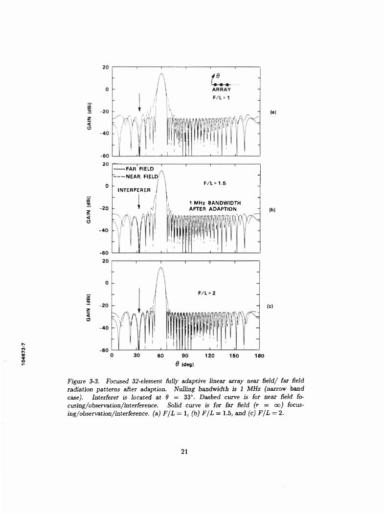
Consider the case of one interference source (J=l). Let an interferer, with power 50 dB above receiver noise at the array output, be located at 6 = 33° both for finite range focused and infinite range focused arrays. Note that the interferer lies on the fifth side lobe to the left of the main beam. Initially, two nulling bandwidths will be considered: B = 1 MHz (narrow band, BLcos6/c = .01) and B = 100 MHz (wide band, BLcosO/c = 1.0).
For B = 1 MHz, the adaptive array radiation patterns, at center frequency 1.3 GHz, are shown in Figure 3-3. Figure 3-3(a) is for a near field range of one aperture diameter (F/L = 1).
17
00
UJ O 3
-10
-20
+ FAR FIELD
O NEAR FIELD
£ -30 2 <
-40 -
-50
T T
*-** •-*-* .~. ^. ^ — -• »* - <*? «• e e e
_® e P
e
e e_
12 16 20
ELEMENT NUMBER
24 28 32
i
Figure 3-1. Amplitude of near Geld and far fieid weights, for a 32-eiement linear array, before nulling. Illumination is for —40 dB Chebyshev array factor. Array element spacing is A/2.
18

i
CO
z < CD
CO
Z -20 <
CO
z < 15
(a)
(b)
(c)
Figure 3-2. 32-element linear array near fieid/far Geld radiation patterns before nulling. Scan angle is 6 = 60° with -40 dB Chebyshev illumination. Array element spacing is A/2. Dashed curve is for near Geld focusing with near Geld observation. Solid curve is for far Geld (r = oo) focusing with far Geld observation, (a) F/L = 1, (b) F/L = 1.5, and (c) F/L = 2.
19

Figures 3-3(b) and 3-3(c) are for near field ranges of l.bL and 2L, respectively. For each case, the adaptive cancellation ratio was computed to be 50 dB. This is expected because ideal nulling weights are used and there are 32 degrees of freedom available for canceling the interference. The consumption of adaptive array degrees of freedom is depicted in Figure 3-4. It is seen that two eigenvalues are significantly above the receiver noise level. The remaining eigenvalues are at the receiver noise level (0 dB); thus, only two degrees of freedom are engaged. The near field eigenvalues are in good agreement with the corresponding far field eigenvalues indicating that the degrees of freedom are consumed the same. The amplitude of the adaptive array NF/FF weights (wa) is given in Figure 3-5 and good agreement is evident. To show the sensitivity of a near field null to range and angle a two dimensional contour radiation pattern is given in Figure 3-6. The pattern in Figure 3-6 has been computed for the F/L — 1 case.
Next, for £?=100 MHz, the adaptive array radiation patterns are shown in Figure 3-7. Again, for each near field range considered, the adaptive array cancellation ratio was computed to be 50 dB. Since the bandwidth has increased, more degrees of freedom are consumed but there are still ample degrees of freedom remaining. In Figure 3-8, it is seen that six eigenvalues are above the receiver noise level. Equivalently, six degrees of freedom are consumed. This is true both for the near field and far field degrees of freedom. The amplitude of the adaptive array NF/FF weights is depicted in Figure 3-9. Only minor differences between the NF and FF adaptive weights are observed.
To compare near field and far field consumption of the adaptive array degrees of freedom as a function of nulling bandwidth, the dominant eigenvalues of the interference covariance matrix are presented in Figure 3-10 in the range (1 < F/L < 2). Figure 3-10(a) shows near field and far field eigenvalues (Ai, A2, • • •, A7) for F/L = 1. Figures 3-10(b) and 3-10(c) show the corresponding NF and FF eigenvalues for F/L = 1.5 and F/L = 2, respectively. Notice that each of the near field and far field eigenvalues are in good agreement, that is, X^F « AfF, X$F « XFF, • • •, A^ « XFF. It is observed that the near field eigenvalues are not particularly sensitive to range.
3.2.2 Multiple Interferers
To demonstrate the validity of the NF/FF adaptive nulling equivalence for multiple sources, consider the previous array case (N=32) and now where there is a large number of interferers, say J = 31. Let the interferers be uncorrelated and uniformly distributed across the field of view with five-degree spacing covering 5° < 6 < 170°, excluding the main beam region. The quiescent weights and quiescent radiation patterns were shown in Figures 3-1 and 3-2, respectively. The nulling bandwidth is assumed to be 1 MHz. The total amount of interference power before adaption is adjusted to be 50 dB above noise at the array output.
The array NF/FF adaptive radiation patterns, at center frequency 1.3 GHz, are shown in Figure 3-11. It is observed that nulls are formed at the interferer positions for both NF and FF patterns. The NF/FF main beam and side lobe characteristics are approximately equal. The cancellation ratio was computed to be (48.7 dB, 48.4 dB, 48.4 dB, and 48.4 dB) for ranges (F/L = 1, 1.5, 2, and 00), respectively. Note that complete cancellation, C=50 dB, has not been achieved
20
I
CD •o
< (9
CD •D
<
-20
FAR FIELD
NEAR FIELD'
INTERFERER F/L=1.5
1 MHz BANDWIDTH AFTER ADAPTION
60 90 120 160 0 (cleg)
(a)
(b)
- (C)
180
Figure 3-3. Focused 32-element fully adaptive linear array near Geld/ far 6eld radiation patterns after adaption. Nulling bandwidth is 1 MHz (narrow band case). Interferer is located at 6 = 33°. Dashed curve is for near field fo- cusing/observation/interference. SoHd curve is for far Held (r = ooj focus- ing/observation/interference, (a) F/L = 1, (b) F/L = 1.5, and (c) F/L = 2.
21
CD
to w 3 -I < >
S3 UJ
uu -I 1 1 1 1 1 1 1
-6 80 -
F/L=1 60 -
40 1
1 1
20 -
0
m
•eeeeeeeeeeeeeeeeeeeeeeeeeeeei i i i i i i i i
(a)
CD
HI 3 _J < > Z UJ O UJ
100
80
60
40
20 -
0
-10
T 1 1 r 4 + FAR FIELD
O NEAR FIELD
F/L=1.5
1 MHz BANDWIDTH ONE INTERFERER
j i i i i ' ' •
(b)
CD 3. (O UJ 3 _l < > Z UJ O UJ
uu -I 1 1 1 1 1 1 I
80 -
F/L=2 -
60 -
40 * -
20 -
0
m -I I I I I I I 12 16
INDEX
20 24 28
- (c)
32
Figure 3-4. Covariance matrix eigenvalues for focused 32-element fully adaptive lin- ear array. One near Geld/ far field interferer is located at 8 = 33°. Nulling bandwidth is 1 MHz (narrow band case), (a) F/L = 1, (b) F/L = 1.5, and (c) F/L = 2.
22
m •v tu Q
E _i a s <
u
-10
-20
—r
© © © © ©
-r
© ©e © ©©
i
©e© © © ©
T
© ©
I
F/L=1 -
-30 .<P © ©
-40 -
(»)
0
+ FAR FIELD
UJ
-10
-20
" O NEAR FIELD © © ©
F/L=1.5 e©©ffiffi©ffi©©©ffi
®©ffi e©a © m o 6 © ^ 3
Q ^ ® 1 MHz BANDWIDTH © •30 ONE INTERFERER 9 !'
a. Z <
-40
(b)
i
i 12 16 20
ELEMENT NUMBER
24 28 32
(c)
Figure 3-5. Amplitude of focused 32-element linear array weights after nulling. One near Geld/far Beld interferer is located at 6 = 33°. Nulling bandwidth is 1 MHz (narrow band case), (a) F/L = 1, (b) F/L = 1.5, and (c) F/L = 2.
23
UJ
(3 Z < oc
l"t ' I ' I ' I ' I
1 MHz BANDWIDTH
' I ' I^U-r-^ -
- AFTER ADAPTION ^ •••
13 — .^^-30 dBi
-40^. N -
"" / INTERFERER —
12 ^-60 >r
—
11 —
^^^^^-30 dBi IK —
10 ••*•—•—•••• —
I
ARRAY
-
31 32 33
ANGLE, 6 (deg)
34 35
Figure 3-6. Two dimensional near field gain distribution, in the vicinity of an adap- tive null, for the focused 32-element linear array. Interferer is at range F/L = 1 (ri = 11.73 ft) and angle 6{ = 33°. Nulling bandwidth is 1 MHz (narrow band case).
24
I
CD •c
< (9
20
CO
z 3 o
INTERFERER
—i—i—i— FAR FIELD NEAR FIELD
F/L =1.5
100 MHz BANDWIDTH AFTER ADAPTION
CO
z <
-20
(a)
(b)
(c)
Figure 3-7. Focused 32-element fully adaptive linear array near Geld/far Geld ra- diation patterns after adaption. Nulling bandwidth is 100 MHz (wide band case). Interferer is located at 6 = 33°. (a) F/L = 1, (b) F/L = 1.5, and (c) F/L = 2.
25
CD
v> in
100
80
60
40
g 2°
0
-10
100
m 5. 60 in HI 3 < 40
ai S 20
CD
UJ
-I < > Z LU
52 UJ
0
-10
100
_e i
6
i i
-
_ 6 F/L=1 _
6 -
• + - o -
_ 6 ;
e e e _. 1 L
ee i J— ..
eeeeeeee ee © © ©H
.6 + FAR FIELD 6 O NEAR FIELD
F/L=1.5
100 MHz BANDWIDTH ONE INTERFERER
1 I '
(a)
(b)
(c)
g
Figure 3-8. Covariance matrix eigenvalues for focused 32»element fully adaptive lin- ear array. One near Geld/ far Geld interferer is located at6 — 33°. Nulling bandwidth is 100 MHz (wide band case), (a) F/L = 1, (b) F/L = 1.5, and (c) F/L = 2.
26

CD
Q
0.
<
(a)
0
-10 m TJ
HI -20 D 3
-1 -30 0. s < -40
-50
_0 NEAR FIELD. $ e ® ® *e e ® e ® ® ©«
T + FAR FIELD
« ©,
-O .+ 6
® ©
F/L=1.5
100 MHz BANDWIDTH
ONE INTERFERER
*9- (b)
S
m •v. m o 3
Q. s <
-10
-20
•30
-40
-5 0
g$$e®e®©®©©^ ©
_*6
J I I I I L
T r F/L=2
12 16 20 24
ELEMENT NUMBER
28 32
(c)
Figure 3-9. Amplitude of focused 32-element linear array weights after Dulling. One near Geld/'far Geld interferer is located at 0 = 33°. Nulling bandwidth is 100 MHz (wide band case), (a) F/L = 1, (b) F/L = 1.5, and (c) F/L = 2.
27
£0
w LLI
< > Z UJ
a
CO
UJ
D —i < > Z UJ
O
CD
UJ
—i
> Z UJ
UJ
100
80
60
40
20
0
I I I I I •—I 1
*1 A2 ^=^=^^=:rz =^=^="=rr==rI ^^^ ——r^"^—:rz==r~=^~
- sy *3 ^^^ F/L=1
V 7 /
^ K^^ ^^ —— "
^
""" K ^3^-r^
II i i i i i A7
25 50 75
NULLING BANDWIDTH (MHz)
100
(a)
(b)
(c)
Figure 3-10. Dominant covariance matrix eigenvalues for focused 32-element fully adaptive linear array as a function of nulling bandwidth. One near Geld/far Geld interferer is located at 6 = 33°. (a) F/L = 1, (b) F/L = 1.5, and (c) F/L = 2.
28

20
i §
OD •c
<
CD •D
<
m
z 3 o
-20
-40 -
-60
20
n—i—i—i—i 1—i—i—i—i—i—i—i—i 1—i—i—
F/L=1
_l I I lLI_l I L _l_
(8)
-20
-40
-60
20
—i—i—i—i—i—i—i—i—i—i—i—i—i—i—i—i—r FAR FIELD
NEAR FIELD
J I I tilLl I L
AFTER ADAPTION
F/L =1.5
1 MHz BANDWIDTH 31 INTERFERERS
(A0 = 5°)
J 1_
(b)
-20 -
-40 -
-60
T—i—i—i—i—i—i—i—i—i—r i—i—i—i—r-
F/L = 2
j i_
(c)
30 60 90 120
0 (deg)
160 180
Figure 3-11. Focused 32-element fully adaptive linear array near Geld/far Geld radi- ation patterns after adaption. There are 31 interferers with uniform five-degree spac- ing (excluding the main beam region). Nulling bandwidth is 1 MHz. (a) F/L = 1, (b) F/L = 1.5, and (c) F/L = 2.
29

here because the interference is significantly stressing the adaptive array degrees of freedom. This is observed in Figure 3-12 which shows that all of the covariance matrix eigenvalues are above receiver noise. Note that there is good agreement between the NF and FF eigenvalues. Finally, the adaptive array weights are shown in Figure 3-13. Although there is some shape difference between NF and FF weights, their dynamic ranges are similar. It is observed that the dynamic range covered by the weights is increasing with decreasing range.
From the above results, it is concluded that 31 near field (or point source) interferers, arranged equivalently in terms of angle, are equivalent to 31 far field (or plane wave) interferers. A generalization of this statement would be that J near field interferers are equivalent to J far field interferers. This observation is consistent with additional simulations [8] not considered here.
30
t s
100 I I I I I I I I F/L=1 _
n
LU
80
60 o
— + — -I < > Z w O
40
20
O
+ —
+ 9 • -
- 6- 0 -
-10 i
10 0 I I I I I I I I
-—• 80 -66666666666666666G666666<i
F/L=1.5 -
) f UJ D -I < > Z UJ O
60
40
_+ FAR FIELD
_0 NEAR FIELD
1MHz BANDWIDTH
o - + —
o
\: 6.
UJ 20
_ 31 INTERFERERS
0 _i
-10 I I I I I I I I
100 I I I I I I I I F/L=2 -
80 _ ^GGaaaadadftaaaddGGiba©©.^ I n •u
U) UJ 3 -1 < > Z
60
40
O + -
O ~ + —
UJ C3 UJ 20 -
•6 " © -
0 _ -10 i I
12 16 20 24 28
INDEX
32
(a)
(b)
(c)
Figure 3-12. Covariance matrix eigenvalues for focused 32-element fully adaptive linear array. There are 31 NF/FF interferers with uniform five-degree spacing (excluding the main beam region). Nulling bandwidth is 1 MHz. (a) F/L — 1, (b) F/L = 1.5, and (c) F/L = 2.
31

m
111 Q
0. s <
CD TO
LU Q
0.
S <
0
-10
-20
-30
-40
-50
-60
-70
0
-10
-20
-30
-40
-50
-60
-70
0
F/L=1
+ o ++Soo°°
+ + + +^66^?$°Oo0
* + ?° + o + o
+ + 9
- + o
o J L _L _L
—i 1 r
+ FAR FIELD
O NEAR FIELD
+ oO°
+ o + + o'
oc
o ' +
o
J L
-I F/L=1.5
+ + ?
1 MHz BANDWIDTH 31 INTERFERERS
-10
-20 m r> •90 LLI Q
e -40 _j a S < -50
-60
-70
I I T 1 1 r T F/L=2
++to° + + ~o'
o + o
+ + + o + oo° o
•v
J L 8 12 16 20 24 28 32
ELEMENT NUMBER
(a)
(b)
(c)
CO « in m o
Figure 3-13. Amplitude of focused 32-element fully adaptive linear array weights after adaption. There are 31 NF/FF interferers with uniform five-degree spacing (excluding the main beam region). Nulling bandwidth is 1 MHz. (a) F/L = 1, (b) F/L = 1.5, and (c) F/L = 2.
32

4. CONCLUSION
This report has introduced an approach to testing adaptive arrays in the near field. A theory for analyzing the behavior of an adaptive array operating in the presence of near field interference has been developed. The adaptive antenna has been assumed to be a linear array of isotropic receive elements and the near field interference is assumed to radiate from an isotropic antenna (point source). Near field focusing has been used to establish effectively a far field pattern in the near zone. The near field range of interest here has been taken to be one to two aperture diameters of the antenna under test. The theoretical section has addressed both sidelobe canceller and fully adaptive arrays. Equations for calculating the adaptive array covariance matrix and antenna radiation patterns, for near field (spherical wave) and far field (plane wave) interference were given. Numerical simulations of a fully adaptive linear array indicate that the radiation pat- terns, adapted weights, cancellation, and covariance matrix eigenvalues (degrees of freedom) are effectively the same for near field and far field interference. Both single and multiple interference conditions have been analyzed. It has been shown, by example, that J near field interferers in the presence of a near field focused adaptive array are equivalent to J far field interferers in the presence of a far field focused adaptive array. That is, a one-to-one correspondence can be made between near field interferers and far field interferers. The results are expected to be applicable to large planar arrays. Thus, a phased array antenna adaptive nulling system designed for far field conditions can potentially be evaluated more conveniently using near field interference sources. In practice, the interference source antennas can likely be implemented using dipoles or horns. Experimental verification of this technique is desirable.
33
REFERENCES
1. A. D. Yaghjian, "An Overview of Near-Field Antenna Measurements," IEEE Trans. Anten- nas Propagat., Vol. AP-34, No. 1, pp. 30-45, Jan. 1986.
2. R. C. Johnson, H. A. Ecker, R. A. Moore, "Compact Range Techniques and Measurements," IEEE Trans. Antennas Propagat, Vol. AP-17, No. 5, pp. 568-576, Sept. 1969.
3. J. T. Mayhan, "Some Techniques for Evaluating the Bandwidth Characteristics of Adaptive Nulling Systems," IEEE Trans. Antennas Propagat, Vol. AP-27, No. 3, pp. 363-373, May 1979.
4. A. J. Fenn, "Maximizing Jammer Effectiveness for Evaluating the Performance of Adaptive Nulling Array Antennas," IEEE Trans. Antennas Propagat, Vol. AP-33, No. 10, pp. 1131— 1142, Oct. 1985.
5. J. E. Hudson, Adaptive Array Principles, New York: Peter Peregrinus LTD, 1981.
6. A. J. Fenn, "Theory and Analysis of Near Field Adaptive Nulling," 1986 IEEE APS Sym- posium Digest, Vol. 2, IEEE, New York, pp. 579-582, 1986.
7. A. J. Fenn, "Theory and Analysis of Near Field Adaptive Nulling," 1986 Asilomar Conf. on Signals, Systems and Computers, Computer Society Press of the IEEE, Washington, D.C., pp. 105-109, 1986, DTIC AD- A191101.
8. A. J. Fenn, "A Near Field Technique for Phased Array Antenna Adaptive Nulling Perfor- mance Verification," Lincoln Laboratory, Massachusetts Institute of Technology, Project Report SRT-24, Nov. 1987.
9. A. J. Fenn, "Theoretical Near Field Clutter and Interference Cancellation for an Adaptive Phased Array Antenna," 1987 IEEE AP-S Symposium Digest, Vol. 1, IEEE, New York, pp. 46-49, 1987.
10. R. A. Monzingo and T. W. Miller, Introduction to Adaptive Arrays, New York: Wiley, 1980.
11. G. Strang, Linear Algebra and Its Applications, New York: Academic, 1976.
12. W. E. Scharfman and G. August, "Pattern Measurements of Phased-Arrayed Antennas by Focusing into the Near Zone," in Phased Array Antennas, (Proc. of the 1970 Phased Array Antenna Symposium), A. A. Oliner and G. H. Knittel, Eds., Dedham, MA: Artech House, pp. 344-350, 1972.
13. C.H. Walter, Traveling Wave Antennas, New York: Dover, 1970.
35
UNCLASSIFIED SECURITY CLASSIFICATION OF THIS PAGE
REPORT DOCUMENTATION PAGE 1a. REPORT SECURITY CLASSIFICATION
Unclassified
1b. RESTRICTIVE MARKINGS
2a. SECURITY CLASSIFICATION AUTHORITY
2b. DECLASSIFICATION/DOWNGRADING SCHEDULE
3. DISTRIBUTION/AVAILABILITY OF REPORT
Approved for public release; distribution unlimited.
4. PERFORMING ORGANIZATION REPORT NUMBER(S)
Technical Report 822
5. MONITORING ORGANIZATION REPORT NUMBER(S)
ESD-TR-88-233
6a. NAME OF PERFORMING ORGANIZATION
Lincoln Laboratory, MIT
6b. OFFICE SYMBOL (If applicable)
7a. NAME OF MONITORING ORGANIZATION
Electronic Systems Division
6c. ADDRESS (City, State, and Zip Code)
P.O. Box 73 Lexington, MA 02173-0073
7b. ADDRESS (City, State, and Zip Code)
Hanscom AFB, MA 01731
8a. NAME OF FUNDING/SPONSORING ORGANIZATION
Air Force Space Technology Center
8b. OFFICE SYMBOL (If applicable)
AFSTC/SWS
9. PROCUREMENT INSTRUMENT IDENTIFICATION NUMBER
8c. ADDRESS (City, State, and Zip Code)
Kirtland AFB, NM 87117-6008
10. SOURCE OF FUNDING NUMBERS
PROGRAM ELEMENT NO.
6230 IE 63424F
PROJECT NO.
280
TASK NO.
WORK UNIT ACCESSION NO
11. TITLE (Include Security Classification)
Evaluation of Adaptive Phased Array Antenna Far Field Nulling Performance in the Near Field Region
12. PERSONAL AUTHOR(S) Alan J. Fenn
13a. TYPE OF REPORT
Technical Report
13b. TIME COVERED FROM TO.
14. DATE OF REPORT (Year, Month, Day) 19 January 1989
15. PAGE COUNT 46
16. SUPPLEMENTARY NOTATION
None
17 COSATI CODES
FIELD GROUP SUB-GROUP
18. SUBJECT TERMS (Continue on reverse if necessary and identify by block number)
phased arrays antennas adaptive nulling
eigenvalues interference degrees of freedom
near field testing far field testing near field focusing
19. ABSTRACT (Continue on reverse if necessary and identify by block number)
A theory for analyzing the behavior of adaptive phased array antennas illuminated by a near field interference test source is presented. Conventional phased array near field focusing it used to produce an equivalent far field antenna pattern at a range distance of one to two aperture diameters from the adaptive antenna under test. The antenna is assumed to be a linear array of isotropic receive elements. The interferer is assumed to be a bandlimited noise source radiating from an isotropic antenna. The theory is developed for both partially and fully adaptive arrays. Results are presented for the fully adaptive array case with single and multiple interferers which indicate that near field and far field adaptive nulling can be equivalent. The adaptive nulling characteristics studied in detail are the array radiation patterns, adaptive cancellation, covariance matrix eigenvalues, and adaptive array weights.
20. DISTRIBUTION/AVAILABILITY OF ABSTRACT
D UNCLASSIFIED/UNLIMITED B SAME AS RPT. D DTIC USERS
21. ABSTRACT SECURITY CLASSIFICATION Unclassified
22a. NAME OF RESPONSIBLE INDIVIDUAL Lt. Col. Hugh L. Southall, USAF
22b. TELEPHONE (Include Area Code) (617) 981-2330
22c. OFFICE SYMBOL ESD/TML
DD FORM 1473. M MAR 83 APR »drtion may b* uaod until aahauatad. s obaolata.
UNCLASSIFIED SECURITY CLASSIFICATION OF THIS PAGE