Evaluation of ACCESS climate model ocean diagnostics … · Marsland et al.: Evaluation of ACCESS climate model ocean diagnostics in CMIP5 simulations 103 Table 1.Differences in configuration

Australian Meteorological and Oceanographic Journal 63 (2013) 101–119

101

Evaluation of ACCESS climate model ocean diagnostics in CMIP5 simulations

S.J. Marsland1, D. Bi1, P. Uotila1, R. Fiedler2, S.M. Griffies3, K. Lorbacher1, S. O’Farrell1, A. Sullivan1, P. Uhe1, X. Zhou4, A.C. Hirst1

1Centre for Australian Weather and Climate Research, a partnership between CSIRO and the Bureau of Meteorology, Aspendale, Australia.

2Centre for Australian Weather and Climate Research, a partnership between CSIRO and the Bureau of Meteorology, Hobart, Australia.

3NOAA Geophysical Fluid Dynamics Laboratory, Princeton, USA.4Centre for Australian Weather and Climate Research,

a partnership between CSIRO and the Bureau of Meteorology, Melbourne, Australia.

(Manuscript received July 2012; revised April 2013)

Global and regional diagnostics are used to evaluate the ocean performance of the Australian Community Climate and Earth System Simulator coupled model (ACCESS-CM) contributions to the Climate Model Intercomparison Project phase 5 (CMIP5). Two versions of ACCESS-CM have been submitted to CMIP; namely CSIRO-BOM ACCESS1.0 and CSIRO-BOM ACCESS1.3. Results from six of the core CMIP5 experiments (piControl, historical, rcp45, rcp85, 1pctCO2, and abrup-t4xCO2) are evaluated for each of the two ACCESS-CM model versions. Overall, both model versions exhibit a reasonable and stable representation of key diag-nostics of ocean climate performance in the pre-industrial control simulations, including a meridional overturning circulation with North Atlantic Deep Water maxima in the range 22–24 Sv, and a poleward heat transport maximum of around 1.5 PW. For the projected climate change scenarios considered the ACCESS-CM results are in reasonable agreement with responses found in other CMIP models, with the familiar ocean warming, and reduction in strength of meridional over-turning and poleward heat transport. Drifts in the control simulations of both global ocean salinity and global sea-level are opposite in sign for ACCESS1.0 and ACCESS1.3, suggesting problems exist in the closure of the hydrological cycle. The simulation of ocean climate change over the historical period shows a weak response compared to observations, which manifests as a late response of ocean warming and sea level rise starting around 1990 in the model, compared to the mid 1960s in observations. Further historical simulations are underway to ascer-tain if this late response in ACCESS is a robust model feature, or just low fre-quency variability. If the weak response over the historical period proves robust, the likely cause is a too strong cooling from atmospheric aerosols. Broadening the set of experiments to further investigate the relative warming response of the ACCESS-CM to greenhouse gases compared to the cooling response to aerosols is underway, and preliminary results do suggest that the cooling due to aerosols is strong in the historical simulations.

Corresponding author address: Simon Marsland, CSIRO Marine and At-mospheric Research, Private Bag 1, Aspendale, Vic. 3195. Email: [email protected].

102 Australian Meteorological and Oceanographic Journal 63:1 March 2013

ACCESS-CM are given in Bi et al. (2013a), and summarised here in Table 1 for completeness.

Coupled model contributions to CMIP5 provide an opportunity to evaluate an extensive set of key global and regional diagnostics of ocean performance relevant to the climate system. Our choice of model diagnostics, while not comprehensive, is aimed to illustrate the ACCESS-CM performance in terms of key integrals of global ocean climate (e.g. meridional overturning circulation and poleward heat transport), that demonstrate both the level of stability of the control simulations, and the response to climate change forcing scenarios. We benefit from the availability of a large suite of outputs as was recommended by the World Climate Research Program Climate Variability and Predictability (CLIVAR) Working Group on Ocean Model Development (WGOMD) to the development of the CMIP5 protocols (Griffies et al. 2009a). Our choice of diagnostics is further guided by past studies that evaluate forced ocean climate models (e.g. Marsland et al. 2003, Griffies et al. 2009b) and the ocean components of other CMIP coupled climate models (e.g. Griffies et al. 2005, Gnanadesikan et al. 2006, Griffies et al. 2011, Danabasoglu et al. 2012).

This paper is arranged by the following topics: (1) evolution of the ocean temperature and salinity fields; (2) global and regional diagnostics of mass and heat transport, and (3) selected depth-integrated properties representative of ocean climate change. Lastly, a summary of the desirable aspects of the ACCESS-CM ocean model performance, the relative strengths and weaknesses of ACCESS1.0 compared to ACCESS1.3, and the known weaknesses in the formulation and performance of both model versions are discussed.

Temperature and salinity

The stability of sea surface temperature (SST) evolution for the piControl and historical simulations, and the spatial patterns of SST bias, are discussed by Bi et al. (2013a). They find a small warming trend in SST over the 500 year piControl simulation of 0.08°C/century in ACCESS1.0, and a very stable SST evolution in ACCESS1.3 (< 0.01°C/century). The global mean SST evolution for the ACCESS1.0 and ACCESS1.3 piControl, historical, rcp45, rcp85, 1pctCO2, and abrupt4xCO2 simulations are shown in Figs 1(a) and 1(b), respectively. Figs 1(c) and 1(d) show the evolution of model global potential temperature averaged over the full water column. Both the surface and the depth integrated temperature changes in the historical simulations show no discernible ocean warming, relative to the piControl simulation, before the 1990s. This contrasts with observed SST changes and estimates of historical ocean heat content which show a climate change response from at least the 1960s onwards (Domingues et al. 2008). The scenario simulations (rcp45, rcp85, 1pctCO2, abrupt4xCO2) diverge strongly from the piControl, and show similar evolution for each of the respective simulations when comparing ACCESS1.0 to ACCESS1.3.

Introduction

This paper documents the ocean performance of the Australian Community Climate and Earth System Simulator coupled model (ACCESS-CM; Bi et al. 2013a) contributions to the Climate Model Intercomparison Project phase 5 (CMIP5; Taylor et al. 2012). For each of the two submitted ACCESS-CM model versions, namely CSIRO-BOM ACCESS1.0 and CSIRO-BOM ACCESS1.3, results are presented from the six core CMIP5 experiments completed. The ACCESS-CM experiments considered here are referred to according to the nomenclature of Taylor et al. (2012) as the piControl, historical, rcp45, rcp85, 1pctCO2, and abrupt4xCO2 simulations. Details of the experimental design for these six experiments, along with the forcings used, are given in the Dix et al. (2013) paper in this issue of the Australian Meteorological and Oceanographic Journal (AMOJ).

Details of the ACCESS Ocean Model (ACCESS-OM) formulation for CMIP5 are given in Bi et al. (2013b, a). ACCESS-OM comprises the United States (US) National Oceanographic and Atmospheric Administration (NOAA) Geophysical Fluid Dynamics Laboratory (GFDL) Modular Ocean Model version 4.1 (MOM4p1; Griffies 2009), and the US Los Alamos National Laboratory version 4.1 sea-ice model (CICE4.1; Hunke and Lipscomb 2008). ACCESS-OM has previously been used in studies of the rapid mass-induced sea-level response of the global ocean to freshwater input from glacial melt (Lorbacher et al. 2012), and the simulated sea-ice sensitivity to coherent multi-parameter sea-ice model tuning (Uotila et al. 2012). For the purposes of ACCESS-CM, the MOM4p1 and CICE4.1 models are coupled via the French Centre Européen de Recherche et de Formation Avancée en Calcul Scientifique (CERFACS) OASIS-3.25 software (Valcke 2006), as described by Bi and Marsland (2010).

The OASIS-3.25 software also couples ACCESS-OM to the United Kingdom Met Office Unified Model atmospheric model (Collins et al. 2011, Martin et al. 2011, Hewitt et al. 2011), with ACCESS1.0 using the MOSES land surface and vegetation scheme (nine surface types, canopy types alongside bare ground, and prescribed canopy albedos), and ACCESS1.3 using the CABLE land surface and vegetation scheme (13 surface types, canopy above ground allowing for aerodynamic and radiative interactions between canopy and ground, and resolved canopy albedos). The primary changes in the atmosphere model are that ACCESS1.3 uses the prognostic cloud prognostic condensate (PC2) scheme (Wilson et al. 2008), has a radiation scheme that accounts for horizontal cloud inhomogeneity, and includes improved boundary layer physics for the fluxes of momentum, sensible and latent heat. Further details of the atmospheric and land component formulations, and how they differ between ACCESS1.0 and ACCESS1.3, are described elsewhere in this issue (Bi et al. 2013a, Dix et al. 2013, Kowalczyk et al. 2013). Details of the differences in ACCESS-OM configuration between the ACCESS1.0 and ACCESS1.3 versions of the

Marsland et al.: Evaluation of ACCESS climate model ocean diagnostics in CMIP5 simulations 103

Table 1. Differences in configuration of ACCESS-OM between the CSIRO-BOM ACCESS1.0 and ACCESS1.3 CMIP5 contributions. The critical Richardson number parameter (Rc) used in the KPP Surface Boundary Layer Scheme (Large et al. 1994) was halved in ACCESS1.0 with respect to ACCESS1.3, to improve (increase) the amplitude of the power spectrum of interan-nual variability of the ENSO signal in the ACCESS1.0 simulations. Sea-ice albedos (αc, αb , and αm) were increased for the ACCESS1.3 simulation so as to produce thicker (more realistic) Arctic sea-ice (Uotila et al. 2013, Bi et al. 2013a). The time step (s) of the ocean model (∆to), the sea-ice model (∆ti), and the ocean/sea-ice coupling frequency (∆toi), were concurrently reduced to 1800 s as necessary to overcome intermittent computational instabilities in the ACCESS1.3 simulations.

Symbol Description ACCESS1.0 ACCESS1.3

Surface Boundary Layer Scheme

Rc Critical Richardson number 0.15 0.30

Sea-ice albedos

αc Cold deep snow albedo on sea ice 0.78 0.84

αb Bare ice albedo 0.61 0.68

αm Melting deep snow albedo on sea-ice 0.65 0.72

Time discretisation

∆to Ocean model time step 3600 s 3600/1800 s∆ti Sea-ice model time step 3600 s 3600/1800 s∆toi Ocean/sea-ice coupling interval 3600 s 3600/1800 s

Fig. 1. Time series of annual mean globally averaged sea surface temperature (°C; top), and annual mean total ocean depth aver-aged potential temperature (°C; bottom), for ACCESS1.0 (left) and ACCESS1.3 (right). Lines in each panel are for the piCon-trol (black), historical (red), rcp45 (green), rcp85 (blue), 1pctCO2 (yellow), and abrupt4xCO2 (magenta) simulations.


is volume conserving. However, the surface freshwater fluxes are real mass fluxes, which allows the ocean volume to change according to the balance of precipitation, evaporation, ocean to sea-ice freezing, sea-ice to ocean melting, and river runoff from land. The surface freshwater flux imbalance for the piControl and historical simulations is shown in Bi et al. (2013a). They conclude that the hydrological cycle is not balanced in both ACCESS1.0 and ACCESS1.3, which remains a challenge for future development of the ACCESS-CM. Compared to the respective piControl simulations, there is little difference in the evolution of total ocean salinity in the historical experiments, while all the scenario runs show some freshening relative to their respective piControl simulations, with the exception of the ACCESS1.3 abrupt4xCO2 experiment.

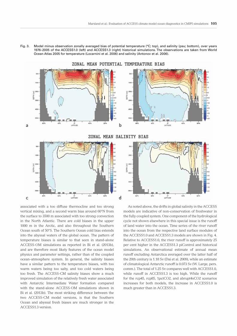
The zonally averaged global potential temperature and salinity biases over the period 1976–2005 of the ACCESS historical simulations, with respect to World Ocean Atlas 2009 (Locarnini et al. 2010, Antonov et al. 2010), are shown in Fig 3. Overall, the bias features are similar when comparing ACCESS1.0 and ACCESS1.3. There is a general warm bias across the tropics and subtropics in the upper 1500 m

The sea surface salinity (SSS; Figs 2(a) and 2(b)) of the piControl and historical simulations, along with the corresponding spatial patterns of SSS bias, are discussed by Bi et al. (2013a). They find the SSS time series reaches a quasi-equilibrium in the later stages of both the ACCESS1.0 and ACCESS1.3 piControl simulations, after recovering from a freshening ‘coupling shock’ in the spin-up phase. The historical simulations show contrasting behavior between ACCESS1.0 (which shows a weak freshening relative to the piControl) and ACCESS1.3 (which shows a weak increase in SSS). All scenario simulations show large freshening, that are of similar magnitude across the two models. This similarity between the two model versions does not hold when considering the time series for the full-depth averaged salinity (Figs 2(c) and 2(d)).

As discussed by Bi et al. (2013a), in the control simulations, there is a small freshening in ACCESS1.0, and a stronger salinification in ACCESS1.3, for the total ocean depth integrated salinity. This is attributed to non-closure in the hydrological cycling between the various model sub-components. As described in Bi et al. (2013b), the ACCESS-OM uses the Boussinesq approximation so the ocean interior

Fig. 2. As in Fig. 1, but for globally averaged sea surface salinity (psu; top), and total ocean depth averaged salinity (psu; bottom).


As noted above, the drifts in global salinity in the ACCESS models are indicative of non-conservation of freshwater in the fully coupled system. One component of the hydrological cycle not shown elsewhere in this special issue is the runoff of land water into the ocean. Time series of the river runoff into the ocean from the respective land surface modules of the ACCESS1.0 and ACCESS1.3 models are shown in Fig. 4. Relative to ACCESS1.0, the river runoff is approximately 25 per cent higher in the ACCESS1.3 piControl and historical simulations. An observational estimate of annual mean runoff excluding Antarctica averaged over the latter half of the 20th century is 1.18 Sv (Dai et al. 2009), while an estimate of climatological Antarctic runoff is 0.073 Sv (W. Large, pers. comm.). The total of 1.25 Sv compares well with ACCESS1.0, while runoff in ACCESS1.3 is too high. While the runoff for the rcp45, rcp85, 1pctCO2, and abrupt4xCO2 scenarios increases for both models, the increase in ACCESS1.0 is much greater than in ACCESS1.3.

associated with a too diffuse thermocline and too strong vertical mixing, and a second warm bias around 60°N from the surface to 3500 m associated with too strong convection in the North Atlantic. There are cold biases in the upper 1000 m in the Arctic, and also throughout the Southern Ocean south of 50°S. The Southern Ocean cold bias extends into the abyssal waters of the global ocean. The pattern of temperature biases is similar to that seen in stand-alone ACCESS-OM simulations as reported in Bi et al. (2013b), and are therefore most likely features of the ocean model physics and parameter settings, rather than of the coupled ocean–atmosphere system. In general, the salinity biases have a similar pattern to the temperature biases, with too warm waters being too salty, and too cold waters being too fresh. The ACCESS-CM salinity biases show a much improved simulation of the relatively fresh water associated with Antarctic Intermediate Water formation compared with the stand-alone ACCESS-OM simulations shown in Bi et al. (2013b). The most striking difference between the two ACCESS-CM model versions, is that the Southern Ocean and abyssal fresh biases are much stronger in the ACCESS1.3 version.

Fig. 3. Model minus observation zonally averaged bias of potential temperature (°C; top), and salinity (psu; bottom), over years 1976–2005 of the ACCESS1.0 (left) and ACCESS1.3 (right) historical simulations. The observations are taken from World Ocean Atlas 2005 for temperature (Locarnini et al. 2006) and salinity (Antonov et al. 2006).


more energetic than the ACCESS1.0 simulation, especially so for the strength and eastward extension of the Kuroshio Current, and for the strength of the ACC (see also the model globally integrated kinetic energy evolution).

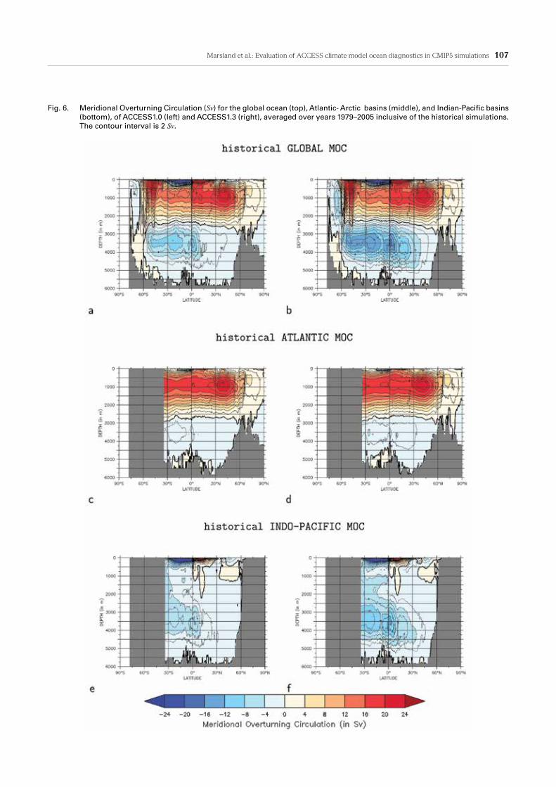
The zonally averaged global Meridional Overtuning Circulation (MOC), Atlantic MOC, and Indo-Pacific MOC, averaged over the period 1979–2005 inclusive of the historical simulations, are shown in Fig. 6. The Antarctic Bottom Water (AABW) cell (below 2500 m) is notably stronger in the ACCESS1.3 simulation, when compared with ACCESS1.0, for each of the global, Atlantic, and Indo-Pacific Basins. The AABW cell also penetrates much further northwards into

Transports of mass and heat

The time mean barotropic (depth integrated) stream function of the ACCESS1.0 and ACCESS1.3 historical simulations (1979–2005 inclusive) are shown in Fig. 5. We note that the barotropic stream function for the corresponding period in the piControl simulations is very similar (not shown). The ACCESS1.0 and ACCESS1.3 patterns are qualitatively similar, and show typical features that are to be expected in ocean simulations, such as the Gulf Stream, Kuroshio Current, Antarctic Circumpolar Current (ACC), and subtropical gyres. In general, the ACCESS1.3 simulation is

Fig. 4. Time series of the ten-year running mean of the globally integrated annual mean runoff from land to ocean (Sv) for ACCESS1.0 (left) and ACCESS1.3 (right).

Fig. 5. Barotropic stream function (Sv) of ACCESS1.0 (left) and ACCESS1.3 (right), averaged over the years 1979–2005 inclusive of the historical simulations.


Fig. 6. Meridional Overturning Circulation (Sv) for the global ocean (top), Atlantic- Arctic basins (middle), and Indian-Pacific basins (bottom), of ACCESS1.0 (left) and ACCESS1.3 (right), averaged over years 1979–2005 inclusive of the historical simulations. The contour interval is 2 Sv.


The ACCESS1.0 and ACCESS1.3 zonally averaged northward heat transports are shown for the global ocean in Figs 8(a) and 8(b), for the Atlantic–Arctic Basins in Figs 8(c) and 8(d), and for the Indo-Pacific Basins in Figs 8(e) and 8(f). Several features are notable: first, with respect to the piControl simulation, the global northward heat transport is larger in the northern hemisphere for the historical simulations, while for all other scenario simulations (rcp45, rcp85, 1pctCO2, and abrupt4xCO2) it is smaller; second, that the same relationship among the various simulations occurs at all latitudes in the Atlantic Ocean; and third, that both the piControl and historical simulations show stronger southward (negative) heat transports south of 10°S than the other scenario runs in the Indo-Pacific Basin. The higher poleward heat transport in the historical simulations relative to piControl is consistent with the higher strength of MOC/AMOC that was seen in Fig. 7 prior to 1990.

The global and Atlantic zonally averaged northward heat transports are compared with in situ observational estimates (Rintoul and Wunsch 1991, Macdonald and Wunsch 1996, Johns et al. 1997), and estimates derived from the top of the atmosphere, using ECMWF reanalysis data (Gibson et al. 1997) to remove atmospheric heat transport, as part of the Earth Radiation Budget Experiment (Trenberth and Solomon 1994). For the historical simulations both the global and Atlantic modelled heat transports often (but not always) lie within the error bars of the observations, although for the global case the heat transports are notably too weak in the southern hemisphere. Weak southern ocean heat transport is a common feature in coupled ocean–atmosphere models, and has previously been seen in the CMIP3 models (Randall 2007).

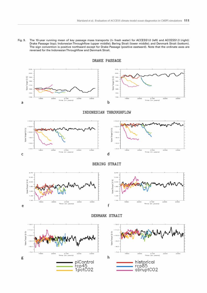
The time series of a selection of key passage transports for the ACCESS1.0 and ACCESS1.3 CMIP5 simulations are shown in Fig. 9. The Drake Passage transport (Figs 9(a) and 9(b)) is a standard measure of ACC strength. Over the period 1850–2005 of the piControl simulations, the Drake Passage transport mean and standard deviation (temporal trend removed) is 161.7 ± 1.5 Sv for ACCESS1.0, and 192.7 ± 2.7 Sv for ACCESS1.3. The transport in ACCESS1.0 is slightly larger than the observation of Cunningham et al. (2003) of 136.7 ± 7.8 Sv, but within the range of a more recent estimate of 154 ± 38 Sv (Firing et al. 2011), while for ACCESS1.3 the transport is clearly too strong. In ACCESS1.3, the Drake Passage transport decreases with respect to the piControl simulation for the rcp45, rcp85, 1pctCO2, and abrupt4xCO2 scenarios, with little change in the historical experiment. In contrast, there is little change of Drake Passage transport in ACCESS1.0 for all the scenario experiments.

The Indonesian Throughflow (ITF) transport is also relatively stable in the piControl and historical simulations, with a strength of 11.0 ± 1.1 (11.0 ± 1.1) and 9.4 ± 0.9 (9.4 ± 1.9 Sv) for ACCESS1.0 (ACCESS1.3), respectively (Figs 9(c) and 9(d)). This is somewhat weaker than a recent observational estimate of 15 Sv (Gordon et al. 2009). For the climate change scenario runs the ITF shows a strong reduction, to as low as

the Pacific Basin in ACCESS1.3. Also, the Southern Ocean Cell (SOC; south of 60°S) is stronger in ACCESS1.3 than in ACCESS1.0 in the global MOC. The stronger formation of AABW in ACCESS1.3 is consistent with the stronger deep cold bias in that model (Fig. 3(b)).

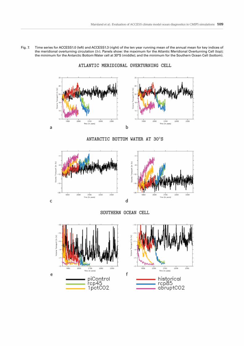
Time series of the AABW and SOC cells of the MOC are shown in Fig. 7. Both the AABW cell (Figs 7(c) and 7(d)) and the SOC (Figs 7(e) and 7(f)) show a considerable decrease in the strength of overturning in the scenario experiments (rcp45, rcp85, 1pctCO2, abrupt4xCO2) when compared to the piControl and historical simulations. This slow-down in overturning in the Southern Ocean has also previously been seen in climate change scenario experiments (e.g. Bi et al. 2001, Sen Gupta et al. 2009).

The Atlantic Meridional Overturning Cell (AMOC; centred at approximately 40°N and 900 m depth in Figs 6(c) and 6(d)) is qualitatively similar when comparing ACCESS1.0 and ACCESS1.3 over the last decades of the historical simulations. In particular, the AMOC maximum is approximately 22 Sv in both models. This similarity can also be seen in the time series of the AMOC, as shown in Figs 7(a) and 7(b). and the corresponding period in the piControl simulations.

For both ACCESS1.0 and ACCESS1.3, the AMOC maximum is typically in the range 19–28 Sv throughout the piControl and historical simulations. The strength of AMOC in the ACCESS historical simulations is in reasonable agreement with other CMIP5 models that typically lie in the range 15–25 Sv (Weaver et al., 2012).

For the historical simulations it can be seen that the AMOC maximum is generally increasing throughout the twentieth century until around 1990 (Fig. 7(a) and 7(b)). This increase is consistent with an increase in both global and north Atlantic maximum poleward heat transport until 1990 in both ACCESS historical simulations, followed by a decrease after 1990 (not shown). An ensemble of simulations is in preparation, which will help to ascertain if the late warming response is a robust feature of the ACCESS model, or just low frequency variability. From 1990 onwards, the ACCESS historical simulations show a sharp decline in AMOC strength. The weakening in the strength of the AMOC in the late period of the historical simulations for both models continues into the rcp45 and rcp85 experiments, a familiar result for coupled climate models as seen in both CMIP3 (Schmittner et al. 2005) and CMIP5 (Weaver et al. 2012) models.

An observational estimate of AMOC strength from the Rapid Climate Change (RAPID) array of moored instruments at 26.5°N is 18.7 ± 5.6 Sv (Cunningham et al. 2007). The mean and standard deviation (temporal trend removed) for the 1979–2005 period of the historical simulations is 18.8 ± 1.08 Sv for ACCESS1.0 and 19.6 ± 0.92 Sv for ACCESS1.3. Both the model and observed estimates of variability are for annual averages. While the ACCESS models are in good agreement with the mean of the RAPID observations, they do underestimate the interannual variability.


Fig. 7. Time series for ACCESS1.0 (left) and ACCESS1.3 (right) of the ten year running mean of the annual mean for key indices of the meridional overturning circulation (Sv). Panels show: the maximum for the Atlantic Meridional Overturning Cell (top); the minimum for the Antarctic Bottom Water cell at 30°S (middle); and the minimum for the Southern Ocean Cell (bottom).


Fig. 8. The zonally averaged northward heat transport (PW) of ACCESS1.0 (left) and ACCESS1.3 (right): for the global ocean (top); for the Atlantic and Arctic basins (middle); and for the Indian and Pacific basins (bottom). Note that the time averages are for 1979–2005 for the piControl and historical simulations, and for the final 20-year period for all other simulations. Red error bars denote in situ observational estimates from Rintoul and Wunsch (1991), Macdonald and Wunsch (1996), and Johns et al. (1997). Black error bars show 1988 estimates derived from the top of the atmosphere, using ECMWF reanalysis data (Gibson et al. 1997) to remove atmospheric heat transport, as part of the Earth Radiation Budget Experiment and are taken from Trenberth and Solomon (1994).


Fig. 9. The 10-year running mean of key passage mass transports (Sv fresh water) for ACCESS1.0 (left) and ACCESS1.3 (right): Drake Passage (top); Indonesian Throughflow (upper middle); Bering Strait (lower middle); and Denmark Strait (bottom). The sign convention is positive northward except for Drake Passage (positive eastward). Note that the ordinate axes are reversed for the Indonesian Throughflow and Denmark Strait.


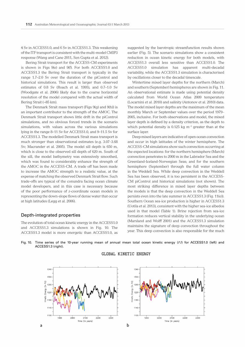
suggested by the barotropic streamfunction results shown earlier (Fig. 5). The scenario simulations show a consistent reduction in ocean kinetic energy for both models, with ACCESS1.3 overall less sensitive than ACCESS1.0. The ACCESS1.0 simulation has apparent multi-decadal variability, while the ACCESS1.3 simulation is characterised by oscillations closer to the decadal timescale.

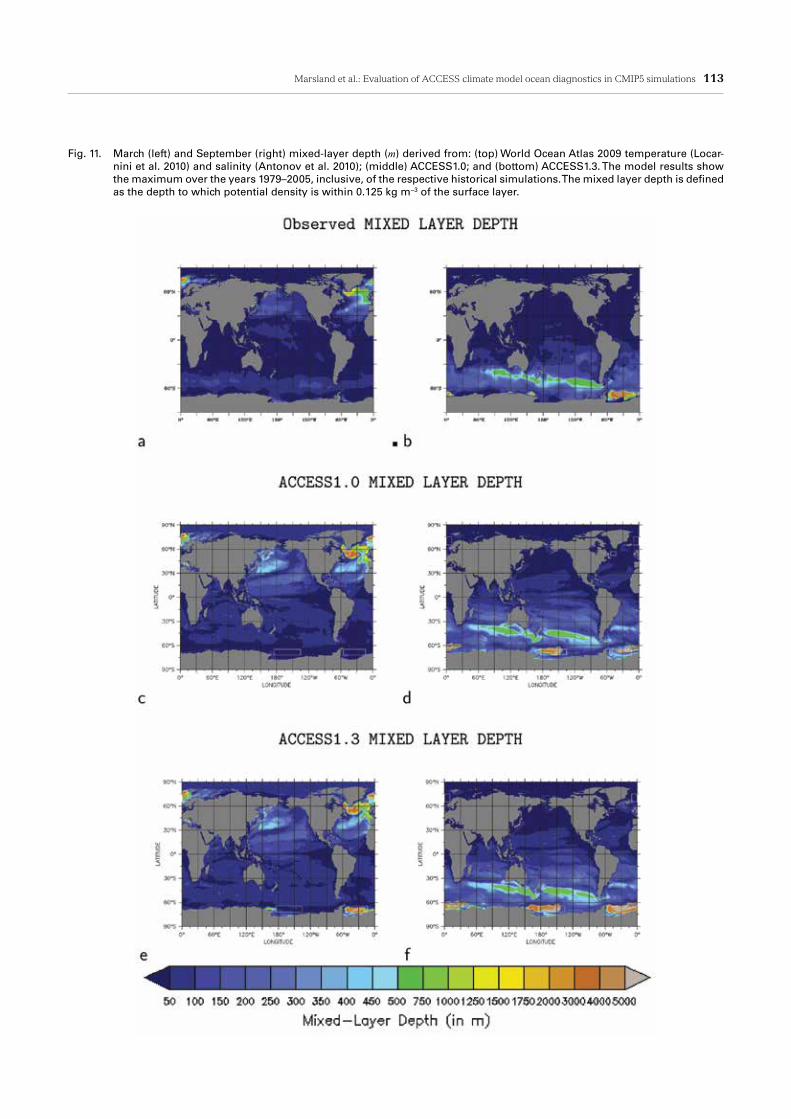
Wintertime mixed layer depths for the northern (March) and southern (September) hemispheres are shown in Fig. 11. An observational estimate is made using potential density calculated from World Ocean Atlas 2009 temperature (Locarnini et al. 2010) and salinity (Antonov et al. 2010) data. The model mixed layer depths are the maximum of the mean monthly March or September values over the period 1979–2005, inclusive. For both observations and model, the mixed layer depth is defined by a density criterion, as the depth to which potential density is 0.125 kg m−3 greater than at the surface layer.

Deep mixed layers are indicative of open ocean convection and occur in high latitudes of the winter hemisphere. The ACCESS-CM simulations show such convection occurring at the expected locations: for the northern hemisphere (March) convection penetrates to 2000 m in the Labrador Sea and the Greenland-Iceland-Norwegian Seas; and for the southern hemisphere (September) through the full water column in the Weddell Sea. While deep convection in the Weddell Sea has been observed, it is too persistent in the ACCESS-CM piControl and historical simulations (not shown). The most striking difference in mixed layer depths between the models is that the deep convection in the Weddell Sea persists even into the late summer in ACCESS1.3 (Fig. 11(e)). Southern Ocean sea-ice production is higher in ACCESS1.3 (Uotila et al. 2013), consistent with the higher sea-ice albedos used in that model (Table 1). Brine rejection from sea-ice formation reduces vertical stability in the underlying ocean (Marsland and Wolff 2001) and the ACCESS1.3 simulation maintains the signature of deep convection throughout the year. This deep convection is also responsible for the much

4 Sv in ACCESS1.0, and 6 Sv in ACCESS1.3. This weakening of the ITF transport is consistent with the multi-model CMIP3 response (Wang and Cane 2011, Sen Gupta et al. 2012).

Bering Strait transport for the ACCESS-CM experiments is shown in Figs 9(e) and 9(f). For both ACCESS1.0 and ACCESS1.3 the Bering Strait transport is typically in the range 1.7–2.0 Sv over the duration of the piControl and historical simulations. This result is larger than observed estimates of 0.8 Sv (Roach et al. 1995), and 0.7–1.0 Sv (Woodgate et al. 2006) likely due to the coarse horizontal resolution of the model compared with the actual width of Bering Strait (~85 km).

The Denmark Strait mass transport (Figs 9(g) and 9(h)) is an important contributor to the strength of the AMOC. The Denmark Strait transport shows little drift in the piControl simulations, and no obvious forced trends in the scenario simulations, with values across the various simulations lying in the range 8–11 Sv for ACCESS1.0, and 9–11.5 Sv for ACCESS1.3. The modelled Denmark Strait mass transport is much stronger than observational estimates (e.g. 3.07–3.68 Sv; Macrander et al. 2005). The model sill depth is 650 m, which is close to the observed sill depth of 620 m. South of the sill, the model bathymetry was extensively smoothed, which was found to considerably enhance the strength of the AMOC in the ACCESS-CM. A trade off has been made to increase the AMOC strength to a realistic value, at the expense of matching the observed Denmark Strait flow. Such trade-offs are typical of the conundra facing ocean climate model developers, and in this case is necessary because of the poor performance of z-coordinate ocean models in representing the down-slope flows of dense water that occur at high latitudes (Legg et al. 2006).

Depth-integrated properties

The evolution of total ocean kinetic energy in the ACCESS1.0 and ACCESS1.3 simulations is shown in Fig. 10. The ACCESS1.3 model is more energetic than ACCESS1.0, as

Fig. 10. Time series of the 10-year running mean of annual mean total ocean kinetic energy (PJ) for ACCESS1.0 (left) and ACCESS1.3 (right).


Fig. 11. March (left) and September (right) mixed-layer depth (m) derived from: (top) World Ocean Atlas 2009 temperature (Locar-nini et al. 2010) and salinity (Antonov et al. 2010); (middle) ACCESS1.0; and (bottom) ACCESS1.3. The model results show the maximum over the years 1979–2005, inclusive, of the respective historical simulations. The mixed layer depth is defined as the depth to which potential density is within 0.125 kg m−3 of the surface layer.


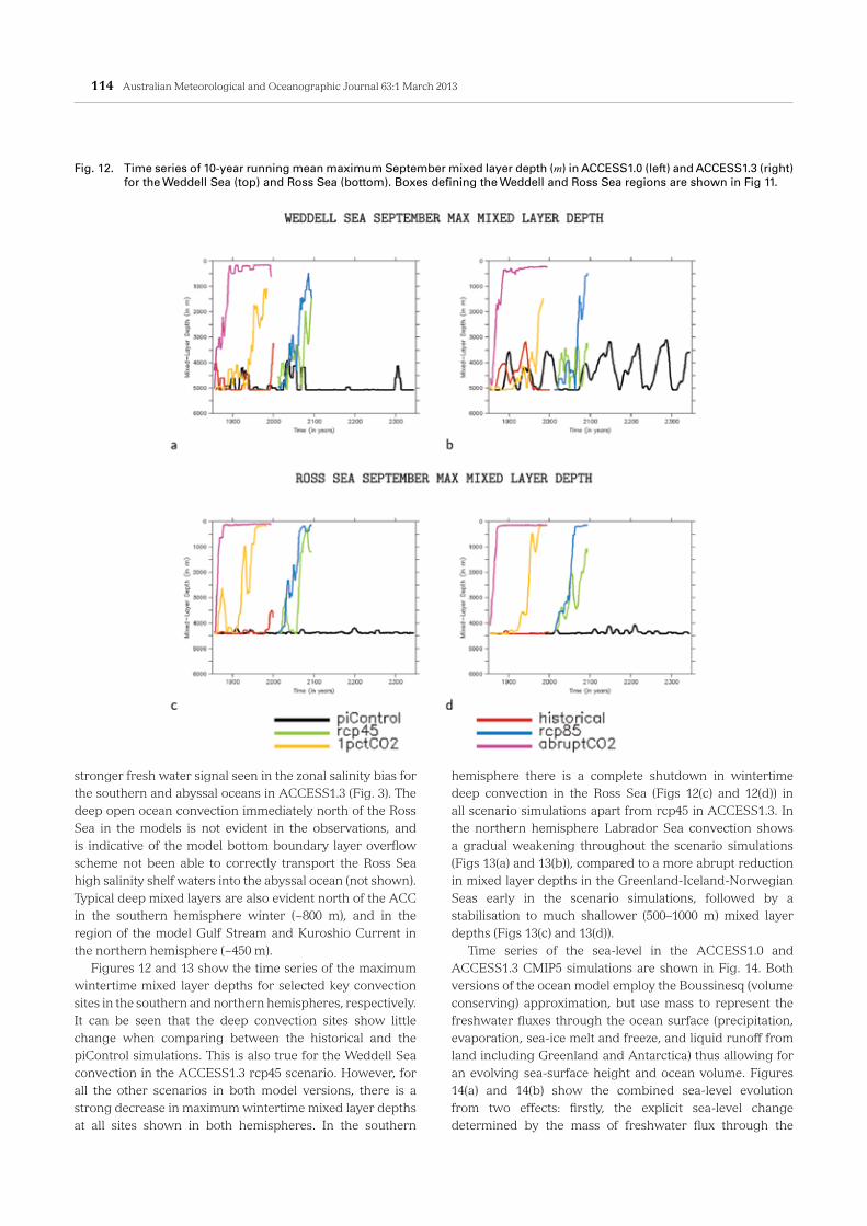
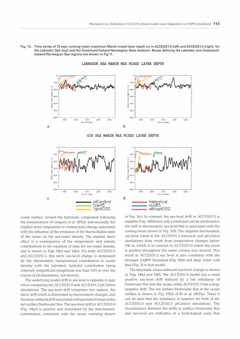
hemisphere there is a complete shutdown in wintertime deep convection in the Ross Sea (Figs 12(c) and 12(d)) in all scenario simulations apart from rcp45 in ACCESS1.3. In the northern hemisphere Labrador Sea convection shows a gradual weakening throughout the scenario simulations (Figs 13(a) and 13(b)), compared to a more abrupt reduction in mixed layer depths in the Greenland-Iceland-Norwegian Seas early in the scenario simulations, followed by a stabilisation to much shallower (500–1000 m) mixed layer depths (Figs 13(c) and 13(d)).

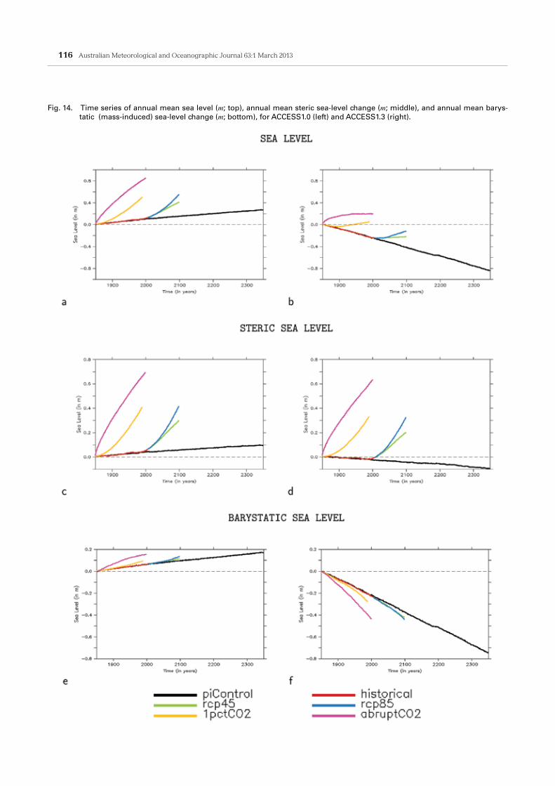
Time series of the sea-level in the ACCESS1.0 and ACCESS1.3 CMIP5 simulations are shown in Fig. 14. Both versions of the ocean model employ the Boussinesq (volume conserving) approximation, but use mass to represent the freshwater fluxes through the ocean surface (precipitation, evaporation, sea-ice melt and freeze, and liquid runoff from land including Greenland and Antarctica) thus allowing for an evolving sea-surface height and ocean volume. Figures 14(a) and 14(b) show the combined sea-level evolution from two effects: firstly, the explicit sea-level change determined by the mass of freshwater flux through the

stronger fresh water signal seen in the zonal salinity bias for the southern and abyssal oceans in ACCESS1.3 (Fig. 3). The deep open ocean convection immediately north of the Ross Sea in the models is not evident in the observations, and is indicative of the model bottom boundary layer overflow scheme not been able to correctly transport the Ross Sea high salinity shelf waters into the abyssal ocean (not shown). Typical deep mixed layers are also evident north of the ACC in the southern hemisphere winter (~800 m), and in the region of the model Gulf Stream and Kuroshio Current in the northern hemisphere (~450 m).

Figures 12 and 13 show the time series of the maximum wintertime mixed layer depths for selected key convection sites in the southern and northern hemispheres, respectively. It can be seen that the deep convection sites show little change when comparing between the historical and the piControl simulations. This is also true for the Weddell Sea convection in the ACCESS1.3 rcp45 scenario. However, for all the other scenarios in both model versions, there is a strong decrease in maximum wintertime mixed layer depths at all sites shown in both hemispheres. In the southern

Fig. 12. Time series of 10-year running mean maximum September mixed layer depth (m) in ACCESS1.0 (left) and ACCESS1.3 (right) for the Weddell Sea (top) and Ross Sea (bottom). Boxes defining the Weddell and Ross Sea regions are shown in Fig 11.


in Fig. 1(c). In contrast, the sea-level drift in ACCESS1.3 is negative (Fig. 14(b)) and only a small part can be attributed to the drift in thermosteric sea level that is associated with the cooling trend shown in Fig. 1(d). The negative thermosteric sea-level trend in the ACCESS1.3 historical and piControl simulations does result from temperature changes below 700 m, which is in contrast to ACCESS1.0 where the trend is positive throughout the water column (not shown). This trend in ACCESS1.3 sea level is also consistent with the stronger AABW formation (Fig. 6(b)) and deep water cold bias (Fig. 3) in that model.

The barystatic (mass-induced) sea-level change is shown in Figs 14(e) and 14(f). The ACCESS1.0 model has a small positive sea-level drift induced by a net imbalance of freshwater flux into the ocean, while ACCESS1.3 has a large negative drift. The net surface freshwater flux at the ocean surface is shown in Fig. 15(b) of Bi et al. (2013a). There it can be seen that the imbalance is negative for both of the ACCESS1.0 and ACCESS1.3 piControl simulations. The inconsistency between the drifts in surface freshwater flux and sea-level are indicative of a hydrological cycle that

ocean surface, termed the barystatic component following the nomenclature of Gregory et al. (2012); and secondly, the implied steric (expansion or contraction) change associated with the influence of the evolution of the thermohaline state of the ocean on the sea-water density. The implied steric effect is a consequence of the temperature and salinity contributions to the equation of state for sea-water density, and is shown in Figs 14(c) and 14(d). For both ACCESS1.0 and ACCESS1.3, this steric sea-level change is dominated by the thermosteric (temperature) contribution to ocean density, with the halosteric (salinity) contribution being relatively insignificant (magnitude less than 0.01 m over the course of all simulations, not shown).

The underlying model drift in sea level is opposite in sign when comparing the ACCESS1.0 and ACCESS1.3 piControl simulations. The sea-level drift comprises two aspects, the steric drift which is dominated by thermosteric changes, and the mass-induced drift associated with persistent biases in the net surface freshwater flux. The sea-level drift in ACCESS1.0 (Fig. 14(a)) is positive and dominated by the thermosteric contribution, consistent with the ocean warming shown

Fig. 13. Time series of 10-year running mean maximum March mixed layer depth (m) in ACCESS1.0 (left) and ACCESS1.3 (right) for the Labrador Sea (top) and the Greenland-Iceland-Norwegian Seas (bottom). Boxes defining the Labrador and Greenland-Iceland-Norwegian Sea regions are shown in Fig 11.


Fig. 14. Time series of annual mean sea level (m; top), annual mean steric sea-level change (m; middle), and annual mean barys-tatic (mass-induced) sea-level change (m; bottom), for ACCESS1.0 (left) and ACCESS1.3 (right).


ocean response, such as the Drake Passage transport (Figs 9(a) and 9(b)), do suggest that there is large scope for tuning climate simulations outside of the ocean.

Overall, the large-scale ocean behaviour is consistent with observations, with a reasonable representation of ocean circulation (Fig. 5), Atlantic overturning circulation (Fig. 6), and meridional heat transport (Fig. 8). These are properties of fundamental importance for climate simulations, and it is pleasing to see that the ACCESS-CM models generally compare well against a selection of CMIP5 models in comparative skill scores for global and Australian climate as shown by Watterson et al. (2013).

Interpretation of some of the ocean results is perplexing. Despite the strong climate change signals seen in the rcp45, rcp85, 1pctCO2, and abrupt4xCO2 simulations, the historical simulations are surprisingly insensitive relative to the piControl simulations. This is especially so for the evolution of ocean temperature and the steric sea-level changes (Figs 1 and 14, respectively). Indeed, for the poleward heat transports, the response of the historical simulations is opposite in sign when compared to the other scenario runs, with respect to the piControl simulations (Fig. 8). However, examination of the reduction in MOC strength (Fig. 7) and thermosteric sea-level rise (Fig. 15) do show the expected elements of ocean climate response to historical climate change in the latter part (post 1990) of the historical simulations. However, the reduction in MOC strength starts later than in other CMIP models, and the thermosteric warming occurs later than in observations.

This late response to external forcing in the historical simulations gives an overall impression of a weak ocean response to climate change in the ACCESS historical simulations when compared to the piControl. One possibility is that, since only one historical simulation is considered here for each model version, it is feasible that low frequency variability in the ocean interior has by

is not properly closed. The large barystatic sea-level drift in ACCESS1.3 is not unique for models contributing to CMIP5; for example the CNRM-CM5.1 model shows a drift of –0.21 m/century (Voldoire et al. 2012). Figure 15 shows a comparison of the thermosteric sea-level change in the ACCESS historical simulations with an estimate derived from observations (Domingues et al. 2008). Although the model underestimates late twentieth century thermosteric sea-level rise, with no trend evident prior to 1990, it is encouraging that the slope of the simulated and observed lines are similar over the final 20 years of the historical simulation.

A comparison of sea-level change for the respective climate scenario simulations between the ACCESS1.0 and ACCESS1.3 suites of simulations shows: a weak response in the historical simulation relative to the piControl simulation; and a much stronger response that is similar for each pair of the rcp45, rcp85, 1pctCO2, and abrupt4xCO2 simulations. Once again, this is a familiar result for the simulations considered here and is also seen, for example, in the time series of ocean temperature (Fig. 1) and the MOC (Fig. 7).

Discussion and conclusions

Contributions of model results to CMIP5 underpin much of the assessment of climate projection under preparation for the Intergovernmental Panel on Climate Change 5th Assessment Report. Given the wide societal interest in climate change and its possible future effects, the submission of the CSIRO-BOM ACCESS1.0 and ACCESS1.3 models carries a significant responsibility. The ACCESS-CM is a recent development and the CMIP5 contributions are a major first test of model performance. The ocean climate diagnostic suite presented here is useful for evaluating the quality of the simulations, and also for assessing the future evolution of climate under the prescribed CMIP5 forcing protocols. The results presented here should be considered as a complement to other analyses of ACCESS1.0 and ACCESS1.3 that appear in this special issue: namely the sea-ice study of Uotila et al. (2013); the overview of Bi et al. (2013a); the atmospheric model assessments of Dix et al. (2013), Rashid et al. (2013a) and Watterson et al. (2013); the El Niño Southern Oscillation analysis of Rashid et al. (2013b); and the land surface evaluation of Kowalczyk et al. (2013).

There are a number of caveats to consider when interpreting the diagnostics presented here. There are minor differences between the ocean and sea-ice components of ACCESS1.0 and ACCESS1.3: in the ocean surface boundary layer scheme (change in Richardson number in KPP scheme) and in the sea-ice albedos. As described elsewhere in this issue, the major differences between ACCESS1.0 and ACCESS1.3 are in the atmospheric and land surface components (Bi et al. 2013a, Dix et al. 2013, Kowalczyk et al. 2013). Differences such as the cloud and land surface schemes hamper the interpretation of differences purely resulting from changes in the ocean components of ACCESS1.0 and ACCESS1.3. However, large differences in

Fig. 15. Annual mean thermosteric sea-level rise (mm) refer-enced to 1963 from Domingues et al. (2008) (black solid with error range black dashed), ACCESS1.0 (red), and ACCESS1.3 (green).


Bi, D., and Marsland, S.J. 2010. Australian Climate Ocean Model (Aus-COM) Users Guide, The Centre for Australian Weather and Climate Research. CAWCR Technical Report No. 027, 82pp.

Bi, D., Dix, M., Marsland, S.J., O’Farrell, S., Rashid, H., Uotila, P., Hirst, A.C., Kowalczyk, E., Golebiewski, M., Sullivan, A., Hailin, Y., Hanna, N., Franklin, C., Sun, Z., Vohralik, P., Watterson, I., Zhou, X., Fiedler, R., Collier, M., Ma, Y., Noonan, J., Stevens, L., Uhe, P., Zhu, H., Hill, R., Harris, C., Griffies, S., and Puri K. 2013a. The ACCESS coupled model: Description, Control Climate and Preliminary Validation. Aust. Met. Oceanogr. J., 63, 41–64.

Bi, D., Marsland, S.J., Uotila, P., OFarrell, S., Fielder, R., Sullivan, A., Griffies, S.M., Zhou, X., and Hirst, A.C. 2013b, ACCESS-OM: the Ocean and Sea Ice Core of the ACCESS Coupled Model. Aust. Met. Oceanogr. J., 63, 213–32.

Bryan, K. 1996. The steric component of sea level rise associated with en-hanced greenhouse warming: a model study. Clim. Dyn., 12, 545–55.

Collins, W.J., Bellouin, N., Doutriaux-Boucher, M., Gedney, N., Halloran, P., Hinton, T., Hughes, J., Jones, C.D., Joshi, M., Liddicoat, S., Martin, G., OConnor, F., Rae, J., Senior, C., Sitch, S., Totterdell, I., Wiltshire, A., and Woodward, S. 2011. Development and evaluation of an Earth-Sys-tem model – HadGEM2. Geoscientific Model Development, 4, 1051–75, doi:10.5194/gmd-4-1051-2011.

Cunningham, S.A., Alderson, S.G., King, B.A., and Brandon, M.A. 2003, Transport and variability of the Antarctic Circumpolar Current in Drake Passage. J. Geophys. Res., 108, 8084, doi:10.1029/2001JC001147.

Cunningham, S.A., Kanzow, T., Rayner, D., Baringer, M.O., Johns, W.E., Marotzke, J., Longworth, H.R., Grant, E.M., Hirschi, J.J.-M., Beal, L.M., Meineni, C.S., and Bryden, H.L. 2007. Temporal Variability of the Atlantic Meridional Overturning Circulation at 26.5°N. Science, 317, 935–8, DOI:10.1126/science.1141304.

Dai, A., Qian, T., Trenberth, K., and Milliman, K. 2009. Changes in con-tinental freshwater discharge from 1948–2004. J. Clim., 22, 2773–91.

Danabasoglu, G., Bates, S.C., Briegleb, B.P., Jayne, S.R., Jochum, M., Large, W.G., Peacock. S., Yeager, S.G. 2012. The CCSM4 Ocean Com-ponent. J. Clim., 25, 1361–89.

Dix, M., Vohralik, P., Bi, D., Rashid, H., Marsland, S., OFarrell, S., Uotila, P., Hirst, T., Kowalczyk, E., Sullivan, A., Yan, H., Franklin, C., Sun, Z., Watterson, I., Collier, M., Noonan, J., Stevens, L., Uhe, P., and Puri, K. 2013. The ACCESS coupled model: Documentation of core CMIP5 simulations and initial results. Aust. Met. Oceanogr. J., 63, 83–99.

Domingues, C.M., Church, J.A., White, N.J., Geckler, P.J., Wijffels, S.E., Baker, P.M., and Dunn, J.R. 2008. Improved estimates of upper-ocean warming and multi-decadal sea level rise. Nature, 453, doi:10.1038/nature07080.

Firing, Y.L., Chereskin, T.K., and Mazloff, M.R. 2011. Vertical structure and transport of the Antarctic Circumpolar Current in Drake Pas-sage from direct velocity observations, J. Geophys. Res., 116, C08015, doi:10.1029/2011JC006999.

Gibson, J.K., Kållberg, P., Uppala, S., Hernandez, A., Nomura, A., and Ser-rano, E. 1997. ERA description. ECMWF Re-analysis Proj. Rep. Ser. 1, Eur. Cent. for Medium-Range Weather Forecasts, Reading, England.

Gnanadesikan, A., Dixon, K.W., Griffies, S.M., Balaji, V., Barreiro, M., Beesley, J.A., Cooke, W.F., Delworth, T.L., Gerdes, R., Harrison, M.J., Held, I.M., Hurlin, W.J., Lee, H.C., Liang, Z., Nong, G., Pacanowski, R.C., Rosati, A., Russell, J.L., Samuels, B.L., Song, Q., Spelman, M.J., Stouffer, R.J., Sweeney, C., Vecchi, G.A., Winton, M., Wittenberg, A.T., Zeng, F., Zhang, R., and Dunne, J.P. 2006. GFDL’s CM2 Global Coupled Climate Models. Part II: The baseline ocean simulation. J. Clim., 19, doi:10.1175/JCLI3630.1.

Gordon A.L., Sprintall, J., Van Aken, H.M., Susanto, D., Wijffels, S., Mol-card, R., Field, A., Pranowo, W., and Wirasantosa, S. 2009. The Indo-nesian throughflow during 2004–2006 as observed by the INSTANT program, Dyn. Atmos. and Oceans, 50, 115–28.

Gregory, J., White, N., Church, J., Bierkens, M., Box, M., Van den Broeke, M., Cogley, G., Fettweis, X., Hanna, E., Huybrechts, P., Konikow, L., Leclercq, P., Marzeion, B., Oerlemans, J., Tamisiea, M., Wada, Y., Wake, L., and Van de Wal, R. 2012. Twentieth-century global-mean sea-level rise: is the whole greater than the sum of the parts? J. Clim., doi:10.1175/JCLI- D-12-00319.1, in press.

Griffies, S.M., Gnanadesikan, A., Dixon, K.W., Dunne, J.P., Gerdes, R.,. Harrison, M.J., Rosati, A., Russell, J.L., Samuels, B.L., Spelman, M.J., Winton, M., and Zhang, R. 2005. Formulation of an ocean model for

chance dominated the climate response. Although such an explanation is unlikely, since the same behaviour is seen in both of the ACCESS models, new historical simulations are underway to investigate this possibility. Another possibility is that the ACCESS-CM cooling response to atmospheric aerosols is too strong relative to the warming response from Greenhouse gases. Preliminary investigation of atmosphere only simulations using SST climatology suggests that the ACCESS model does indeed have a strong sensitivity to aerosol forcing. Further simulations are underway using the CMIP5 protocols for single forcing and other experiments designed for climate change detection and attribution studies (e.g. AnthropogenicAerosols-only and No-AnthropogenicAerosols). Results from these studies will be reported elsewhere, but it is our hope that they shed light on the questions raised here.

Finally, the opposite responses between ACCESS1.0 and ACCESS1.3 global salinity (Figs 2(c) and 2(d)) and the sea-level evolution related to surface mass fluxes (Figs 14(e) and 14(f)) suggest problems in the closure of the hydrological cycle in both model versions. It remains a challenge for ACCESS-CM to produce a fully closed hydrological cycle across all model components.

Acknowledgments.

This work has been undertaken as part of the Australian Climate Change Science Program, funded jointly by the Department of Climate Change and Energy Efficiency, the Bureau of Meteorology and CSIRO. This work was supported by the NCI National Facility at the ANU. We acknowledge the World Climate Research Programme’s Working Group on Coupled Modelling, which is responsible for CMIP, and we thank the ACCESS climate modeling group for producing and making available their model output. For CMIP the U.S. Department of Energy’s Program for Climate Model Diagnosis and Intercomparison provides coordinating support and led development of software infrastructure in partnership with the Global Organization for Earth System Science Portals. We are grateful to Alex Sen Gupta for his very helpful reviews of this work.

ReferencesAdcroft, A. and Campin, J.-M. 2004. Rescaled height coordinates for ac-

curate representation of free-surface flows in ocean circulation mod-els, Ocean Modelling, 7, 269–84.

Antonov, J., Locarnini, R., Boyer, T., Mishonov, A., and Garcia, H. 2006. World Ocean Atlas 2005, vol. 2: Salinity. U.S. Government Printing Of-fice 62, NOAA Atlas NESDIS, Washington, DC, 182 pp.

Antonov, J.I., Seidov, D., Boyer, T.P., Locarnini, R.A., Mishonov, A.V., Garcia, H.E. Baranova, O.K., Zweng, M.M., and Johnson, D.R. 2010. World Ocean Atlas 2009, Volume 2: Salinity, S. Levitus, Ed., NOAA Atlas NESDIS 69, U.S. Government Printing Office, Washington, D.C., 184 pp.

Bi, D., Budd, W.F., Hirst, A.C., and Wu, X. 2001. Collapse and reorganisa-tion of the Southern Ocean overturning under global warming in a coupled model. Geophys. Res. Lett., 28, 3927–30.


els, J. Computational Physics, 126, 251–75, doi:10.1006/jcph.1996.0136.Randall, D.A., R.A. Wood, S. Bony, R. Colman, T. Fichefet, J. Fyfe, V. Katt-

sov, A. Pitman, J. Shukla, J. Srinivasan, R.J. Stouffer, A. Sumi and K.E. Taylor. 2007. Cilmate Models and Their Evaluation. In: Climate Change 2007: The Physical Science Basis. Contribution of Working Group I to the Fourth Assessment Report of the Intergovernmental Panel on Cli-mate Change [Solomon, S., D. Qin, M. Manning, Z. Chen, M. Marquis, K.B. Averyt, M.Tignor and H.L. Miller (eds.)]. Cambridge University Press, Cambridge, United Kingdom and New York, NY, USA.

Rashid, H.A., Hirst, A.C., and Dix, M. 2013a. Atmospheric circulations in the ACCESS model simulations for CMIP5: Present day simulations and future projections. Aust. Met. Oceanogr. J., 63, 145–60.

Rashid, H.A., Sullivan, A., Hirst, A.C., Bi, D., Zhou, X., and Marsland, S.J. 2013b. Evaluation of simulated El Niño-Southern Oscillation in AC-CESS coupled model simulations for CMIP5, Aust. Met. Oceanogr. J., 63, 161–80.

Rintoul S.R. and Wunsch C. 1991. Mass, heat, oxygen and nutrient fluxes and budgets in the North Atlantic Ocean. Deep Sea Res., 38, Suppl. 1, 355–77.

Roach, A.T., Aagaard, K., Pease, C.H., Salo, S.A., Weingartner, T., Pavlov, V., and Kulakov, M. 1995. Direct measurements of transport and water properties through the Bering Strait. J. Geophys. Res., 100, 18443–57, doi:10.1029/95JC01673.

Sen Gupta, A., Santoso, A., Taschetto, A.S., Ummenhofer, C.C., Trevena, J., and England, M.H. 2009. Projected Changes to the Southern Hemi-sphere Ocean and Sea Ice in the IPCC AR4 Climate Models. J. Clim., 22, 3047–78.

Sen Gupta, A., Ganachaud, A., Mcgregor, S., Brown, J. N., and Muir, L. 2012. Drivers of the projected changes to the Pacific Ocean equatorial circulation. Geophys. Res. Lett., 39, L09605, doi:10.1029/2012GL051447.

Schmittner, A., Latif, M., and Schneider, B. 2005. Model projections of the North Atlantic thermohaline circulation for the 21st cen-tury assessed by observations. Geophys. Res. Lett., 32, L23710, doi:10.1029/2005GL024368.

Taylor, K.E., Stouffer, R.J., and Meehl, G.A. 2012. An Overview of CMIP5 and the experiment design. Bull. Am. Meteorol. Soc., 93, doi:10.1175/BAMS-D-11-00094.1.

Trenberth, K.E. and Solomon, A. 1994. The global heat balance: heat transports in the atmosphere and ocean. Clim. Dyn., 10, 107–34.

Uotila, P., O’Farrell, S., Marsland, S.J., and Bi, D. 2012. A sea-ice sensitiv-ity study with an ocean- ice model. Ocean Modelling, 51, 1–18, http://dx.doi.org/10.1016/j.ocemod.2012.04.002.

Uotila, P., O’Farrell, S., Marsland, S.J., and Bi, D. 2013. The sea-ice perfor-mance of the Australian climate models participating in the CMIP5, Aust. Met. Oceanogr. J., 63, 121–43.

Valcke, S. 2006. OASIS3 User Guide (prism 2-5), PRISM-Support Initiative, Report No. 3, CERFACS, Toulouse, France, 64pp.

Voldoire, A., Sanchez-Gomez, E., Salas y Mélia, D., Decharme, B., Cassou, C., Sénési, S., Valcke, S., Beau, A., Alias, A., Chevallier, M., D´equ´e, M., Deshayes, J., Douville, H., Fernandez, E., Madec, G., Maisonnave, E., Moine, M.-P., Planton, S., Saint-Martin, D., Szopa, S., Tyteca, S., Alkama, R., Belamari, S., Braun, A., Coquart, L., and Chauvin, F. 2012. The CNRM-CM5.1 global climate model: description and basic evalu-ation, Clim. Dyn., 31 pp, DOI 10.1007/s00382-011-1259-y.

Wang, D. and Cane, M. 2011. Pacific Shallow Meridional Overturning Cir-culation in a Warming Climate. J. Clim., 24, 6424–39, doi: http://dx.doi.org/10.1175/2011JCLI4100.1.

Watterson, I.G., Hirst, A.C., and Rotstayn, L.D. 2013. A skill-score based evaluation of simulated Australian climate. Aust. Met. Oceanog. J., 63, 181–90.

Weaver, A.J., Jan Sedlácek, J., Eby, M., Alexander, K., Crespin, E., Fichefet, T., Philippon-Berthier, G., Joos, F., Kawamiya, M., Matsumoto, K., Stei-nacher, M., Tachiiri, K., Tokos, K., Yoshimori, M., Zickfeld, and K. Geo-phys. Res. Lett., 39, L20709, doi:10.1029/2012GL053763.

Wilson, D.R., Bushell, A.C., Kerr-Munslow, A.M., Price, J.D., and Mor-crette, C.J. 2008. PC2: A prognostic cloud fraction and condensation scheme. I: Scheme description. Q. J. R. Meteorol. Soc., 134, 2093–107.

Woodgate, R.A., Aagaard, K., and Weingartner, T.J. 2006. Interan-nual changes in the Bering Strait fluxes of volume, heat and fresh-water between 1991 and 2004. Geophys. Res. Lett., 33, L15609, doi:10.1029/2006GL026931.

global climate simulations. Ocean Sci., 1, 45–79.Griffies, S.M. 2009. Elements of MOM4p1, GFDL Ocean Group Tech. Rep.

6, NOAA/Geophysical Fluid Dynamics Laboratory, 444 pp.Griffies, S.M., Biastoch, A., Böning, C., Bryan, F., Danabasoglu, G., Chas-

signet, E.P., England, M.H., Gerdes, R., Haak, H., Hallberg, R.W., Ha-zeleger, W., Jungclaus, J., Large, W.G., Madec, G., Pirani, A., Samuel, B.L., Scheiner, M., Sen Gupta, A., Severijns, C.A., Simmons, H.L., Treguier, A.M., Winton, M., Yeager, S., and Yin, J. 2009a. Coordinated Ocean-ice Reference Experiments (COREs). Ocean Modell., 26, 1–46, doi:10.1016/j.odeanmod.2008.08007.

Griffies, S.M., Adcroft, A.J., Aiki, H., Balaji, V., Bentson, M., Bryan, F., Danabasoglu, G., Denvil, S., Drange, H., England, M., Gregory, J., Hallberg, R.W., Legg, S., Martin, T., McDougall, T., Pirani, A., Schmidt, G., Stevens, D., Taylor, K.E., and Tsujino, H. 2009. Sampling Physical Ocean Fields in WCRP CMIP5 Simulations, ICPO Publication Series 137, WCRP Informal Report No. 3/2009, available from http://www-pcmdi.llnl.gov.

Griffies, S.M., Winton, M., Donner, L.J., Horowitz, L.W., Downes, S.M., Farneti, R., Gnanadesikan, A., Hurlin, W.J., Lee, H.C., Liang, Z., Palter, J.B., Samuels, B.L., Wittenberg, A.T., Wyman, B., Yin, J., and Zadeh, N. 2011. The GFDL CM3 Coupled Climate Model: Characteristics of the ocean and sea ice simulations. J. Clim., 24, doi:10.1175/2011JCLI3964.1.

Hewitt, H.T., Copsey, D., Culverwell, I.D., Harris, C.M., Hill, R.S.R, Keen, A.B., McLaren, A.J., and Hunke, E.C. 2011. Design and implementa-tion of the infrastructure of HadGEM3: the next-generation Met Of-fice climate modelling system. Geoscientific Model Development, 4, 223–53, doi:10.5194/gmd-4-223-2011.

Hunke, E.C., and Lipscomb, W.H. 2008. CICE: the Los Alamos Sea Ice Model Documentation and Software User’s Manual Version 4.0, LA-CC-06-012, 72pp.

Johns W.E., Lee T.N., Zantopp R.J. and Fillenbaum E. 1997. Updated transatlantic heat flux at 26.5°N, WOCE Newsletter, 27, 15–22.

Kowalczyk., E.A. Stevens, L., Law, R.M., Dix, M., Wang, Y.P., Harman, I.N., Haynes, K., Srbinovsky, J., Pak, B., and Ziehn, T. 2013. The land surface model component of ACCESS: description and impact on the simu-lated surface climatology. Aust. Met. Oceanogr. J., 63, 65–82.

Large, W.G., McWilliams, J.C., and Doney, S.C. 1994. Oceanic vertical mixing: A review and a model with a nonlocal boundary layer param-eterization. Rev. Geophys., 32, 363–403.

Large, W.G., and Yeager, S. 2009. The global climatology of an interannu-ally varying air-sea flux data set. Clim. Dyn., 33, 341–364.

Legg, S., Hallberg, R.W., and Girton, J.B. 2006. Comparison of entrain-ment in overflows simulated by z-coordinate, isopycnal and non-hy-drostatic models, Ocean Modell., 11, 69–97.

Locarnini, R, Mishonov, A., Antonov, J., Boyer, T., and Garcia, H. 2006. World Ocean Atlas 2005, Volume 1: Temperature. U.S. Government Printing Office 61, NOAA Atlas NESDIS, Washington, DC, 182 pp.

Locarnini, R.A., Mishonov, A.V., Antonov, J.I., Boyer, T.P., Garcia, H.E. Baranova, O.K., Zweng, M.M., and Johnson, D.R. 2010. World Ocean Atlas 2009, Volume 1: Temperature, S. Levitus, Ed., NOAA Atlas NES-DIS 68, U.S. Government Printing Office, Washington, D.C., 184 pp.

Lorbacher, K., Marsland, S.J., Church, J.A., Griffies, S.M., and Stammer, D. 2012. Rapid barotropic sea level rise from ice sheet melting. J. Geo-phys. Res., 117, C06003, doi:10.1029/2011JC007733.

Macdonald A.M. and Wunsch C. 1996. Oceanic estimates of global ocean heat transport, WOCE Newsletter, 24, 5–6.

Macrander, A., Send, U., Valdimarsson, H., Jónsson, S., and Käse, R.H. 2005. Interannual changes in the overflow from the Nordic Seas into the Atlantic Ocean through Denmark Strait. Geophys. Res. Lett., 32, L06606, doi:10.1029/2004GL021463.

Marsland, S.J. and Wolff, J.-O. 2001. On the sensitivity of Southern Ocean sea ice to the surface fresh water flux: A model study. J. Geophys. Res., 106, 2723–41.

Marsland, S.J., Haak, H., Jungclaus, J.H., Latif, M., and Roske, F. 2003. The Max-Planck- Institute global ocean/sea ice model with orthogonal curvilinear coordinates. Ocean Modell., 5, 91–127, doi:10.1016/S1463-5003(02)00015-X.

Martin, G.M. and coauthors. 2011. The HadGEM2 family of Met Office Unified Model climate configurations. Geoscientific Model Develop-ment, 4, 723–57, doi:10.5194/gmd-4-723-2011.

Murray, R.J. 1996. Explicit generation of orthogonal grids for ocean mod-


Documents

Evaluation of ACCESS climate model ocean diagnostics … · Marsland et al.: Evaluation of ACCESS climate model ocean diagnostics in CMIP5 simulations 103 Table 1.Differences in configuration