Clemson UniversityTigerPrints

All Theses Theses

12-2010

EVALUATION AND ADJUSTMENT OFUSDA WASDE COTTON FORECASTSDavid TysingerClemson University, dtysing@g.clemson.edu

Follow this and additional works at: https://tigerprints.clemson.edu/all_theses

Part of the Agricultural Economics Commons

This Thesis is brought to you for free and open access by the Theses at TigerPrints. It has been accepted for inclusion in All Theses by an authorizedadministrator of TigerPrints. For more information, please contact kokeefe@clemson.edu.

Recommended CitationTysinger, David, "EVALUATION AND ADJUSTMENT OF USDA WASDE COTTON FORECASTS" (2010). All Theses. 975.https://tigerprints.clemson.edu/all_theses/975

EVALUATION AND ADJUSTMENT OF USDA WASDE COTTON FORECASTS

A Thesis

Presented to

the Graduate School of

Clemson University

In Partial Fulfillment

of the Requirements for the Degree

Master of Science

Applied Economics and Statistics

by

David Tysinger

December 2010

Accepted by:

Dr. Olga Isengildina-Massa, Committee Chair

Dr. Patrick Gerard

Dr. William Bridges Jr.

ii

ABSTRACT

The dynamic and volatile nature of agricultural markets causes individuals to rely

on forecasts in their decision-making. WASDE cotton forecasts are shown to be

especially volatile as cotton is one of the most trade dependent commodities in the world.

Therefore, its evaluation requires us to look beyond U.S. WASDE categories and

evaluate forecasts for China and the World.

This study will use data from monthly WASDE balance sheets for upland cotton

for the U.S, China and World over 1985/1986 through 2008/2009 including unpublished

price forecasts. The results of this study will provide information that can be used to

improve the accuracy of USDA cotton forecasts. The proposed study will fill the gap in

knowledge of the level of supply and demand forecast uncertainty and its contribution to

price forecast errors by 1) evaluating all weak-form forecast optimality conditions for the

U.S., China and World balance sheet categories for cotton, including trends in forecast

accuracy; 2) investigating whether errors in forecasts are correlated with the U.S., China

and World balance sheet categories, and 3) identifying a statistical correction of

systematic errors in independent variables of the U.S. cotton price model.

iii

DEDICATION

This work is dedicated to all the friends and faculty at Clemson University who

have not only challenged me to achieve great things but have also provided the

inspiration. They all have made this one of my most enriching experiences. A big thanks

goes to all.

iv

ACKNOWLEDGMENTS

A special thanks goes to the distinguished faculty members that served on my

committee: Professors Patrick Gerard, Olga Isengildina-Massa, William Bridges, Jr.

I would also like to recognize the efforts of Dr. Jim Rieck, Dr. David Willis, Dr.

Richard Dubsky, Dr. Charlie Curtis, Dr. David Hughes, and Cherylene Amidon as they

have provided me much inspiration and enjoyment in my academic pursuit.

v

TABLE OF CONTENTS

Page

TITLE PAGE .................................................................................................................... i

ABSTRACT ..................................................................................................................... ii

DEDICATION ................................................................................................................ iii

ACKNOWLEDGMENTS .............................................................................................. iv

LIST OF TABLES ......................................................................................................... vii

LIST OF FIGURES ......................................................................................................... x

CHAPTER

I. INTRODUCTION ......................................................................................... 1

II. DATA ............................................................................................................ 4

III. METHODS .................................................................................................. 11

Forecast Evaluation Framework ............................................................ 11

Forecast Evaluation Results ................................................................... 13

IV. LEARNING FRAMEWORK ...................................................................... 27

Adjustment Procedure ............................................................................ 27

Validation Measures .............................................................................. 29

Validation of Adjustments ..................................................................... 30

V. SUMMARY AND CONCLUSIONS .......................................................... 38

APPENDICES ............................................................................................................... 70

A: SAS Code for Forecast Adjustment ............................................................. 71

B: Regression Plots of the Test of Bias for U.S. Domestic Use ....................... 73

C: Regression Plots of the Test of Bias for China Ending Stocks .................... 76

D: Regression Plots of the Test of Bias for World Imports .............................. 79

E: Chow Test .................................................................................................... 82

vi

Table of Contents (Continued)

Page

REFERENCES .............................................................................................................. 85

vii

LIST OF TABLES

Table Page

1. Summary of Descriptive Statistics for WASDE Cotton

Forecasts, 1985-2008 ............................................................................. 41

2. Dynamic Test of Bias for WASDE U.S. Cotton Forecasts,

1985-2008 Marketing Years .................................................................. 42

3. Dynamic Test of Bias for WASDE China Cotton Forecasts,

1985-2008 Marketing Years .................................................................. 43

4. Dynamic Test of Bias for WASDE World Cotton Forecasts,

1985-2008 Marketing Years .................................................................. 44

5. Test of Orthogonality for WASDE U.S. Cotton Forecasts,

1985-2008 Marketing Years .................................................................. 45

6. Test of Orthogonality for WASDE China Cotton Forecasts,

1985-2008 Marketing Years .................................................................. 46

7. Test of Orthogonality for WASDE World Cotton Forecasts,

1985-2008 Marketing Years .................................................................. 47

8. Test of Weak Efficiency for WASDE U.S. Cotton Forecasts,

1985-2008 Marketing Years .................................................................. 48

9. Test of Weak Efficiency for WASDE China Cotton Forecasts,

1985-2008 Marketing Years .................................................................. 49

10. Test of Weak Efficiency for WASDE World Cotton Forecasts,

1985-2008 Marketing Years .................................................................. 50

11. Test of Independence of Forecast Revisions for WASDE U.S.

Cotton Forecasts, 1985-2008 Marketing Years ..................................... 51

12. Test of Independence of Forecast Revisions for WASDE China

Cotton Forecasts, 1985-2008 Marketing Years ..................................... 52

13. Test of Independence of Forecast Revisions for WASDE World

Cotton Forecasts, 1985-2008 Marketing Years ..................................... 53

viii

List of Tables (Continued)

Table Page

14. USDA WASDE Forecast Evaluation Summary for

1985-2008 Marketing Years: Most Significant

Categories found within the Forecasting Evaluation

Framework (By Region) ........................................................................ 54

15. Evaluation for the Adjustment of Bias in USDA WASDE

U.S. Domestic Use Forecasts, 1999-2008 Marketing

Years ...................................................................................................... 55

16. Evaluation for the Adjustment of Bias in USDA WASDE

China Ending Stock Forecasts, 1999-2008 Marketing

Years ...................................................................................................... 56

17. Evaluation for the Adjustment of Bias in USDA WASDE

World Import Forecasts, 1999-2008 Marketing Years .......................... 57

18. Evaluation for the Adjustment of Forecast Levels in USDA

WASDE U.S. Production Forecasts, 1999-2008

Marketing Years..................................................................................... 58

19. Evaluation for the Adjustment of Forecast Levels in USDA

WASDE China Import Forecasts, 1999-2008 Marketing

Years ...................................................................................................... 59

20. Evaluation for the Adjustment of Forecast Levels in USDA

WASDE World Import Forecasts, 1999-2008 Marketing

Years ...................................................................................................... 60

21. Evaluation for the Adjustment of Lagged Errors in USDA

WASDE U.S. Domestic Use Forecasts, 1999-2008

Marketing Years..................................................................................... 61

22. Evaluation for the Adjustment of Lagged Errors in USDA

WASDE China Domestic Use Forecasts, 1999-2008

Marketing Years..................................................................................... 62

23. Evaluation for the Adjustment of Lagged Errors in USDA

WASDE World Domestic Use Forecasts, 1999-2008

Marketing Years..................................................................................... 63

ix

List of Tables (Continued)

Table Page

24. Evaluation for the Adjustment of Revisions in USDA

WASDE U.S. Domestic Use Forecasts, 1999-2008

Marketing Years..................................................................................... 64

25. Evaluation for the Adjustment of Revisions in USDA

WASDE China Import Forecasts, 1999-2008

Marketing Years..................................................................................... 65

26. Evaluation for the Adjustment of Revisions in USDA

WASDE World Domestic Use Forecasts, 1999-2008

Marketing Years..................................................................................... 66

x

LIST OF FIGURES

Figure Page

1. WASDE Forecasting Cycle for Cotton 2006/07

Marketing Year ...................................................................................... 67

2. WASDE U.S. Cotton Forecast Estimates over Time,

1985-2008 Marketing Years .................................................................. 68

3. WASDE U.S. Cotton Price Estimates over Time,

1985-2008 Marketing Years .................................................................. 68

4. WASDE China Cotton Forecast Estimates over Time,

1985-2008 Marketing Years .................................................................. 69

5. WASDE World Cotton Forecast Estimates over Time,

1985-2008 Marketing Years .................................................................. 69

CHAPTER ONE

INTRODUCTION

The dynamic and volatile nature of agricultural markets causes individuals to rely

on forecasts in their decision-making. Multiple efforts have been devoted in the recent

literature to improve the models for price forecasting with a special focus on futures price

forecasting (e.g. Lence, Hart, and Hayes, 2009; Ticlavilca, Feuz, and McKee, 2009).

Other recent studies demonstrated a growing concern about changes in the relationship

between futures prices and cash prices in the United States (e.g., Irwin, Garcia and Good,

2007; Timmer, 2009) which would limit the usefulness of futures price information for

the purpose of cash price forecasting by USDA. Most cash price forecasting models rely

on fundamental analysis of supply and demand factors (e.g., Meyer, 1998; Westcott and

Hoffman, 1999; Dawe, 2002; Plato and Chambers, 2004; Schaffer, 2004; Goodwin,

Schnepf, and Dohlman, 2005; Goreux, et al., 2007; Isengildina and MacDonald, 2009).

These models are used for forecasting commodity prices throughout the forecasting cycle

which spans several months before (with a typical start in May) and after (most crops are

finalized by November) the U.S. marketing year. The challenge that many forecasters

face early in the forecasting cycle is having to rely on highly uncertain supply and

demand estimates as inputs in their price forecasting models.

Previous forecast evaluation literature has largely focused on forecast accuracy of

two major components of WASDE balance sheets, production (e.g., Gunnelson, Dobson

and Pamperin, 1972; Thomson, 1974; Isengildina, Irwin, and Good, 2006b) and price

(e.g., Marquardt and McGann, 1977; Just and Rausser, 1981; Irwin, Gerlow and Liu,

2

1994; Sanders and Manfredo, 2002; Egelkraut et al., 2003; Isengildina, Irwin, and Good,

2004). The importance of price forecasts is obvious, given the role price expectations

play in decisions on resource allocation. Production forecasts are important because they

are a major determinant of future supply. Interestingly, the accuracy of most other

categories describing supply and demand forces in WASDE forecasts have been

overlooked in the previous literature. To the best of our knowledge, only one previous

study (Botto et.al., 2006) investigated the accuracy of all U.S. WASDE categories.

Knowledge of supply and demand forecast accuracy is important because these

categories serve as building blocks for price forecast accuracy. Furthermore, supply and

demand estimates are published within a set of other forecasts in WASDE reports that

have been shown to affect the markets (e.g, Colling and Irwin, 1990; Fortenbery and

Sumner, 1993; Baur and Orazem, 1994; Isengildina, Irwin, and Good, 2006a). It is a

commonly held belief of agricultural market participants and analysts that WASDE

forecasts function as the ―benchmark‖ to which other private and public forecasts are

compared. The dominant role of WASDE forecasts is not surprising given the classic

public goods problem of private underinvestment in information, and the critical role that

public information plays in coordinating the beliefs of market participants. Therefore it is

important to ensure that WASDE forecasts provide accurate and reliable information to

the public.

The proposed study will fill the gap in knowledge of the level of supply and

demand forecast uncertainty and its contribution to price forecast errors by 1) evaluating

all weak-form forecast optimality conditions for the U.S., China and World balance sheet

3

categories for cotton, including trends in forecast accuracy; 2) investigating whether

errors in U.S. cotton price and ending stocks forecasts are correlated with the U.S., China

and World balance sheet categories, and 3) identifying a statistical correction of

systematic errors in independent variables of the U.S. cotton price model.

This study will concentrate on USDA cotton forecasts as little is known about

their accuracy. Only a few studies have concentrated on a subset of WASDE categories

for cotton (MacDonald, 2002) or included examination of cotton in studies of WASDE

export forecasts for a number of commodities (MacDonald, 1999 and MacDonald 2005).

In fact, the USDA was legally prohibited from forecasting cotton prices from 1929 to

2008. Although cotton price forecasts were not published, USDA’s Interagency

Commodity Estimates Committee for cotton calculated unpublished price forecasts each

month. The accuracy of these unpublished forecasts should be evaluated as USDA

moves forward with its cotton price forecasting mission. Cotton also presents a challenge

of being one of the most trade dependent U.S. commodities. Therefore, its evaluation will

require us to look beyond U.S. WASDE categories which has not been done before. This

study will use data from monthly WASDE balance sheets for upland cotton for the U.S,

China and the World over 1985/1986 through 2008/2009 including unpublished price

forecasts. The results of this study will provide information that can be used to improve

the accuracy of USDA cotton forecasts. The methodology used in this study can be

directly applied to investigation of trends and potential improvements in forecast

accuracy in other commodities.

.

4

CHAPTER TWO

DATA

WASDE reports are released by the USDA usually between the 9th

and the 12th

of

each month and contain forecasts of supply and demand for most major crops. Supply

and demand estimates are forecasted on a marketing year basis. The first forecast for a

marketing year is released in May preceding the U.S. marketing year. Estimates are

typically finalized 18 months later, by November of the following marketing year for

cotton (Figure 1). USDA WASDE forecasts are considered fixed-event forecasts because

the series of forecasts is related to the same terminal event (yiT), where T is the release

month of the final estimate for the category for the ith

marketing year. The forecast of the

terminal event for month t is denoted as: yit , where t=1, ..., T, and i=1985/86, …,

2008/09. Thus, each subsequent forecast is essentially an update of the previous forecast

as it describes the same terminal event. The WASDE forecasting cycle generates 18

updates (T=19) for each forecasted variable within each marketing year for cotton.

WASDE forecasts for the U.S. and the world follow a balance sheet approach to

account for supply and utilization (see Vogel and Bange (1999) for a detailed description

of the USDA crop forecast generation process). The major components of the supply and

demand balance sheet are beginning stocks, imports and production on the supply side

and domestic use, exports and ending stocks on the demand side. Domestic use is usually

further subdivided based on commodity specific uses. The balance sheet approach means

that individual estimates are cross checked against each other, across commodities and

countries. For example, ―total supply must equal domestic use plus exports and ending

5

stocks. Prices tie both sides of the balance sheet together by rationing available supplies

between competing uses.‖ (Vogel and Bange, p. 10). WASDE price projections describe

marketing year average prices received by farmers, which are based on commodity

models reflecting the supply and demand conditions via stock-to-use ratios, lagged prices

and other variables (Labys, 1973; Wescott and Hoffman, 1999, Isengildina and

MacDonald, 2009). Price forecasts are different from all other WASDE categories as

they are published in the form of an interval to reflect the uncertainty associated with the

estimate. Because analysis of interval forecast accuracy is different from point estimate

accuracy (e.g., Isengildina, Irwin, and Good, 2004), midpoints of price forecasts were

used in this study to be consistent with the rest of the analysis.

The focus of this study is monthly WASDE Balance Sheets for the U.S., China, and

World Upland Cotton for the marketing years of 1985/86 through 2008/09. The final

estimates for cotton supply and demand (19th

forecast for each marketing year) were used

to calculate the descriptive statistics found in Table 1. The descriptive statistics were

calculated for each region for the following categories: beginning stocks, production,

imports, domestic use, exports, ending stocks, and price. The statistics calculated for

each of these categories were, mean, standard deviation, coefficient of variation,

skewness, and kurtosis. According to Timmerman (2006), ―Data availability and data

quality may vary significantly across regions and there can be significant differences

even within each region‖; therefore, coefficients of variation were used to compare the

variability associated with forecasting cotton across regions and across categories within

a region. Coefficients of variation were chosen as the preferred measure of variability

6

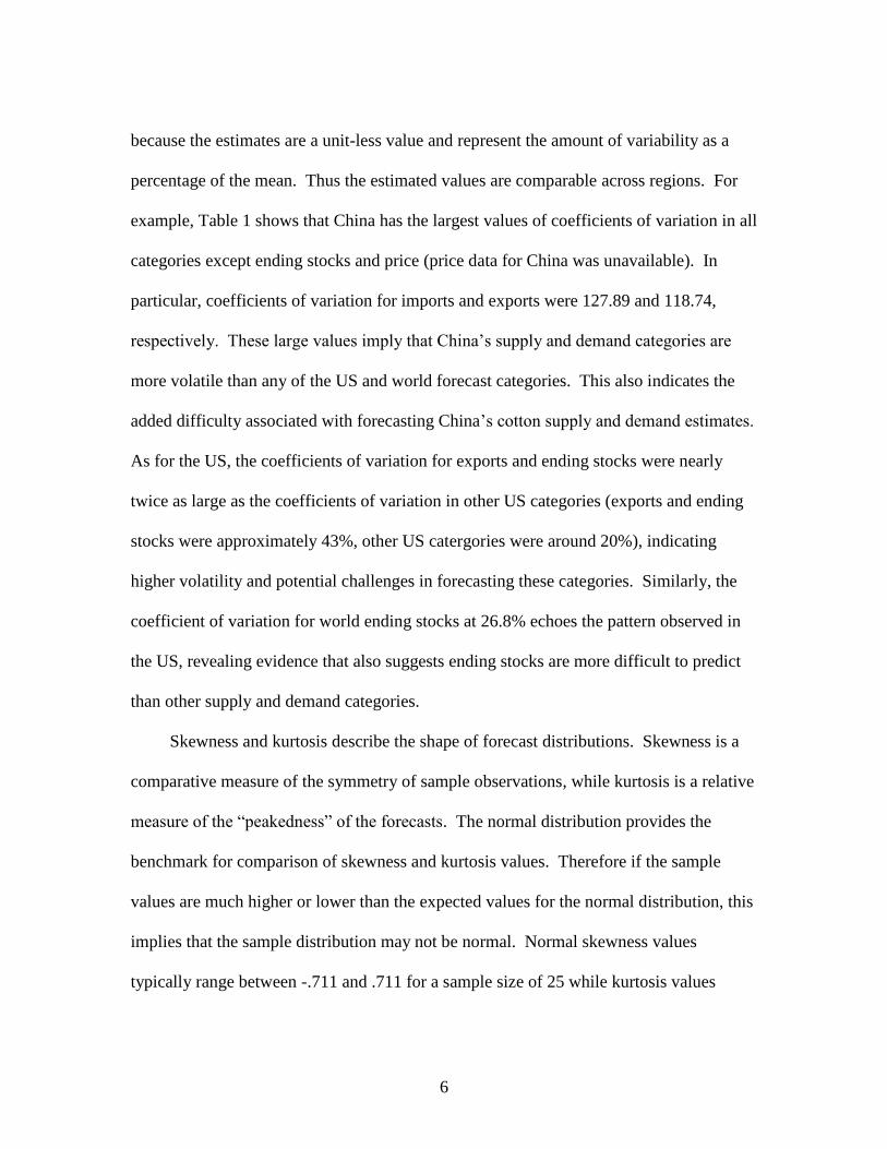
because the estimates are a unit-less value and represent the amount of variability as a

percentage of the mean. Thus the estimated values are comparable across regions. For

example, Table 1 shows that China has the largest values of coefficients of variation in all

categories except ending stocks and price (price data for China was unavailable). In

particular, coefficients of variation for imports and exports were 127.89 and 118.74,

respectively. These large values imply that China’s supply and demand categories are

more volatile than any of the US and world forecast categories. This also indicates the

added difficulty associated with forecasting China’s cotton supply and demand estimates.

As for the US, the coefficients of variation for exports and ending stocks were nearly

twice as large as the coefficients of variation in other US categories (exports and ending

stocks were approximately 43%, other US catergories were around 20%), indicating

higher volatility and potential challenges in forecasting these categories. Similarly, the

coefficient of variation for world ending stocks at 26.8% echoes the pattern observed in

the US, revealing evidence that also suggests ending stocks are more difficult to predict

than other supply and demand categories.

Skewness and kurtosis describe the shape of forecast distributions. Skewness is a

comparative measure of the symmetry of sample observations, while kurtosis is a relative

measure of the ―peakedness‖ of the forecasts. The normal distribution provides the

benchmark for comparison of skewness and kurtosis values. Therefore if the sample

values are much higher or lower than the expected values for the normal distribution, this

implies that the sample distribution may not be normal. Normal skewness values

typically range between -.711 and .711 for a sample size of 25 while kurtosis values

7

generally range between -1 and 1. For the World and China, several WASDE categories

exhibit significant positive skewness and leptokurtic distributions. Specifically,

production, imports, domestic use, and exports were all shown to have positive skewness

and kurtosis values near or above 1. Kurtosis values above 1 implies the distribution

tends to be leptokurtic, displaying a higher ―peak‖ and longer ―fatter tails‖ as compared

to a normal distribution. Skewness values at or above 1 suggests positive skewness

which implies there may be ―upward spikes‖ and/or unpredictably large values within

these categories (Ramirez and Fadiga, 2003). For the World and China, the departures

from normality highlight the extreme difficulty in forecasting these series. In fact, the

Chinese and World production estimates both observed a sizeable increase in 2004 as

Chinese estimates went from 22 million bales to over 29 million bales and World

production estimates went from 94 million bales to over 120 million bales, all within a

single year. In addition to the ―upward spikes‖ in production, Chinese imports realized

the single largest jump in estimates from 2004 to 2005. Chinese imports tripled within a

single year, where in 2004 imports were valued at 6 million bales and over 19 million

bales in 2005. These examples illustrate that Chinese and World forecasts for

production, imports, domestic use, and exports do not follow a normal distribution.

Furthermore, the positive skewness and large kurtosis values tends to show how

unpredictable these categories are and how much volatility within the WASDE Balance

Sheets is the result of these characteristics.

Figures 2-5 display time series plots for the final estimates from WASDE Balance

sheets over of 1985/86 to 2008/09 marketing years. In Figure 2, WASDE U.S. Cotton

8

Estimates over Time, there were two very obvious trends present in the data. In the years

of 1999 to 2008, exports displayed an upward trend and domestic use displayed a

downward trend. Because both domestic use and exports are demand categories within

the WASDE balance sheet they are directly related to one another. Therefore, the

increasing demand for cotton abroad signaled the US to increase the amount of cotton

exported. As a result, ending stocks were found to be very volatile during this time

period, as shown in Figure 2 and referenced in Table 1. Ending stocks saw a sharp rise in

the year 2001 to a value of 7 million bales and then a sharp decline the next two years to

a value of approximately 4 million bales. This volatility was mostly associated with

ending stocks reflecting the difference between total supply and total consumption.

Hence, the unexpected trends in the demand categories of domestic use and exports

increased the overall variability associated with ending stocks.

The time series plot for US cotton price estimates is presented in Figure 3 which

highlights the volatility that has been associated with the forecasts since the year 2000.

Double digit gains and losses for price (measured in ¢/lb) was a frequent occurrence for

the years of 2000-2008. Thus the volatility in price corresponds to trends associated with

domestic use and exports. There also seems to be a corresponding relationship between

ending stocks and price, as price estimates follow a completely reverse pattern of US

ending stock estimates for the same time period. Both categories experienced large

deviations that resulted in a very unstable and unpredictable cotton market.

In Figure 4, China estimates for production and domestic use showed explosive

growth in the years following 2000. Both categories more than doubled in value the final

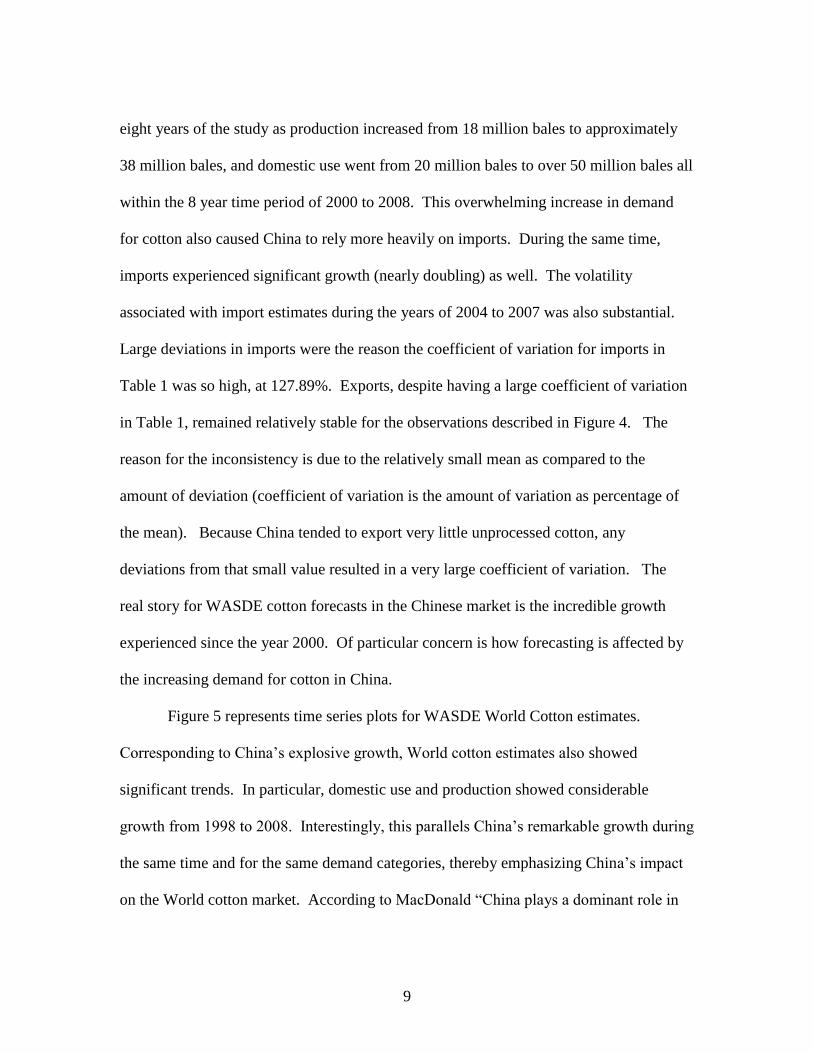
9

eight years of the study as production increased from 18 million bales to approximately

38 million bales, and domestic use went from 20 million bales to over 50 million bales all

within the 8 year time period of 2000 to 2008. This overwhelming increase in demand

for cotton also caused China to rely more heavily on imports. During the same time,

imports experienced significant growth (nearly doubling) as well. The volatility

associated with import estimates during the years of 2004 to 2007 was also substantial.

Large deviations in imports were the reason the coefficient of variation for imports in

Table 1 was so high, at 127.89%. Exports, despite having a large coefficient of variation

in Table 1, remained relatively stable for the observations described in Figure 4. The

reason for the inconsistency is due to the relatively small mean as compared to the

amount of deviation (coefficient of variation is the amount of variation as percentage of

the mean). Because China tended to export very little unprocessed cotton, any

deviations from that small value resulted in a very large coefficient of variation. The

real story for WASDE cotton forecasts in the Chinese market is the incredible growth

experienced since the year 2000. Of particular concern is how forecasting is affected by

the increasing demand for cotton in China.

Figure 5 represents time series plots for WASDE World Cotton estimates.

Corresponding to China’s explosive growth, World cotton estimates also showed

significant trends. In particular, domestic use and production showed considerable

growth from 1998 to 2008. Interestingly, this parallels China’s remarkable growth during

the same time and for the same demand categories, thereby emphasizing China’s impact

on the World cotton market. According to MacDonald ―China plays a dominant role in

10

the world’s cotton economy‖ as China is defined as the world’s largest textile exporter,

has the largest population, and is the world’s second largest economy. There tends to be

a direct relationship with China and World categories. As evidenced through the

categories of domestic use and production, the forecasts follow very similar patterns. In

particular, Chinese production estimates hit a peak in 2005 and declined in 2006 just as

World production estimates hit a peak in 2005 and dropped in 2006. As another

example, domestic use for China continued sharp growth until 2007, which was followed

by a drop in 2008. Similarly, World domestic use exhibited steady growth until 2007 and

fell in 2008. The emerging patterns highlight the effect that China’s cotton economy has

on the rest of the World, especially the volatility associated within China’s balance sheet.

11

CHAPTER THREE

METHODS

Forecast Evaluation Framework:

To evaluate the quality of WASDE forecasts it is necessary to establish a set of

testable properties that an optimal forecast should have. Following Timmerman (2006),

this study assumes that the objective function is of the mean squared error (MSE) type so

the forecasts minimize a symmetric, quadratic loss function. The properties of WASDE

forecasts are investigated using error and revision analysis. For each category, monthly

announcement and marketing year forecast errors and revisions were calculated as

following:

1. eit = y

iT y

it ; t=1,…, T-1; i=1985/86,…,2008/09

1

i i i

t t tr y y ; t=2,…, T; i=1985/86,…,2008/09

where i

te corresponds to the error, i

tr is the revision for a given report month t, and

marketing year i. As defined earlier, i

ty is the forecast for marketing year i released in

month t and i

Ty corresponds to the final estimate for marketing year i, T=19 for cotton.

The fundamental measures of optimal forecasts are bias and efficiency (Diebold and

Lopez, 1998). The test of bias can be performed using a regression:

2. eit = αt + ε

it i=1985/86,…,2008/09

The null hypothesis of an unbiased forecast is α = 0. This hypothesis can be tested using

a t-test. Following Bailey and Brorsen (1998), changes in forecast bias over time can be

detected by including a trend variable:

12

3. eit = αt + βtI + ε

it i=1985/86,…,2008/09, I=1, …, 24.

Where the marketing year, i, relates to the year variable, I, such that the year variable

represents the study period year (i 1984), therefore i=1985/86 corresponds to I=1, and

i=1986/87 corresponds to I=2, and so on. The null hypothesis for an unbiased forecast

over time is that both α = 0 and β = 0.

Weak efficiency tests evaluate whether forecast errors are orthogonal to forecasts

themselves as well as to prior forecast errors (Nordhaus). Thus, weak efficiency is tested

using the following regressions (Pons, 2000):

4. eit = αt + βtyit + εi

t i=1985/86,…,2008/09,

and

5. eit = αt + βteti-1 + εi

t i=1985/86,…,2008/09.

The null hypotheses for efficient forecasts is for β = 0 in equations (4) and (5). These

hypotheses can be tested using a t-test as well.

Furthermore, weak form efficiency of fixed-event forecasts implies independence of

forecast revisions (Nordhaus). According to Nordhaus, if forecasts are weak form

efficient, revisions should follow a random walk. This property can be tested using the

following regressions for each time period t (Isengildina, Irwin, and Good, 2006):

6. rit = γ r

it-1 + εi

t i=1985/86,…,2008/09,

The null hypothesis for efficiency in forecast revisions is γ = 0. For (t=3), γ represents

the slope coefficient of all October revisions made from 1985/86 to 2008/09 regressed

against previous September revisions (t-1=2) for the same respective years.

13

Forecast Evaluation Results:

The quality of WASDE cotton forecasts for the US, China, and the World was

examined over 1985/86 through 2008/09 marketing years. Each month out of the 19

month forecasting cycle was evaluated based on the forecast evaluation framework

described in the previous section. Tables 2-4 show the results of the dynamic test of bias

displayed in equation 3. The results show that intercept terms were found to be

significant throughout U.S. domestic use forecasts. The intercept coefficients represent

the initial bias estimated for the first year of the study period (marketing year of

1984/85). U.S. domestic use forecasts were found to exhibit the initial bias in months 1-

15 of the forecasting cycle. The values of the initial bias were positive which implied

U.S. domestic use was underestimated. Specifically, during the first three months of the

forecasting cycle, the initial bias in domestic use forecasts was estimated at

approximately 1 million bales below the final estimate. Later in that marketing year the

bias decreased to an underestimation of about 200 thousand bales for months 13-15 of the

forecasting cycle. The dynamic component of bias was measured by a trend variable.

The bias in months 1-14 of U.S. domestic use forecasts changed significantly over time

(p < 0.05). The coefficients of trend in each month were negative. Since the coefficients

of the intercept and the trend term were of opposing signs, this suggested that forecast

accuracy improved for the marketing years following 1985/86. The magnitude of this

improvement ranged from 70-80 thousand bales per year for the early months in the

forecasts cycle to about 10-20 thousand bales per year towards the end of the forecasting

cycle.

14

To further study the dynamic component of bias within WASDE forecasts,

regression plots were analyzed on a month-to-month basis to determine how the bias

changed across the forecasting cycle and over time. Regression Plots of the Test of Bias

for US Domestic Use presented in Appendix B demonstrate that while the initial bias in

the first month of the forecasting cycle was 1 million bales, according to Table 2, the

actual amount underestimated in 1985/86 was 1.5 million bales as shown in Appendix B.

Another interesting finding observed in these plots is the fact that toward the end of the

study period the trend dominates the initial bias. Thus, in the five most recent marketing

years, U.S. domestic use was overestimated as demonstrated by the errors months 1-6.

The findings suggest that the biases in these forecasts were changing over time and any

adjustments must take into account the dynamic component.

Table 3, compiled from China forecast errors, shows that beginning stocks,

production, exports, and ending stocks all exhibit significant initial bias (p < 0.05). In

particular, forecasts for beginning stocks, production, and ending stocks display a

negative initial bias (overestimation) whereas forecasts for exports display a positive

initial bias (underestimation). The bias found in the forecasts for ending stocks is the

strongest and most prevalent of all the categories, as 9 out of the 18 months forecasted

show a significant negative initial bias (p < 0.05). In terms of magnitude, months 3-6 of

the forecasting cycle show that ending stocks were overestimated by more than 3 million

bales. Ending stock forecasts for months 14-16, the initial bias had reduced to an

overestimation of approximately 1 million bales. Table 3 also provides evidence that

trend terms in each of the categories were significant. Trends in forecasts for imports and

15

domestic use were found at a significance level of 0.1. Beginning stocks, production,

exports, and ending stocks displayed trends at a significance level of less than 0.01.

Ending stock forecasts were found to exhibit the strongest and most prevalent trends as

15 of the 16 months forecasted were significant with p-values less than 0.05. In Table 3,

ending stock’s coefficients for trend ranged from 350 thousand bales per year for the 3rd

month of the forecasting cycle down to 80 thousand bales per year for the 17th

month.

The values represent the rate at which bias decreased each year, as an increasing trend in

the forecasting cycle implies improvements in the forecasts when the signs of the

intercept coefficients are negative.

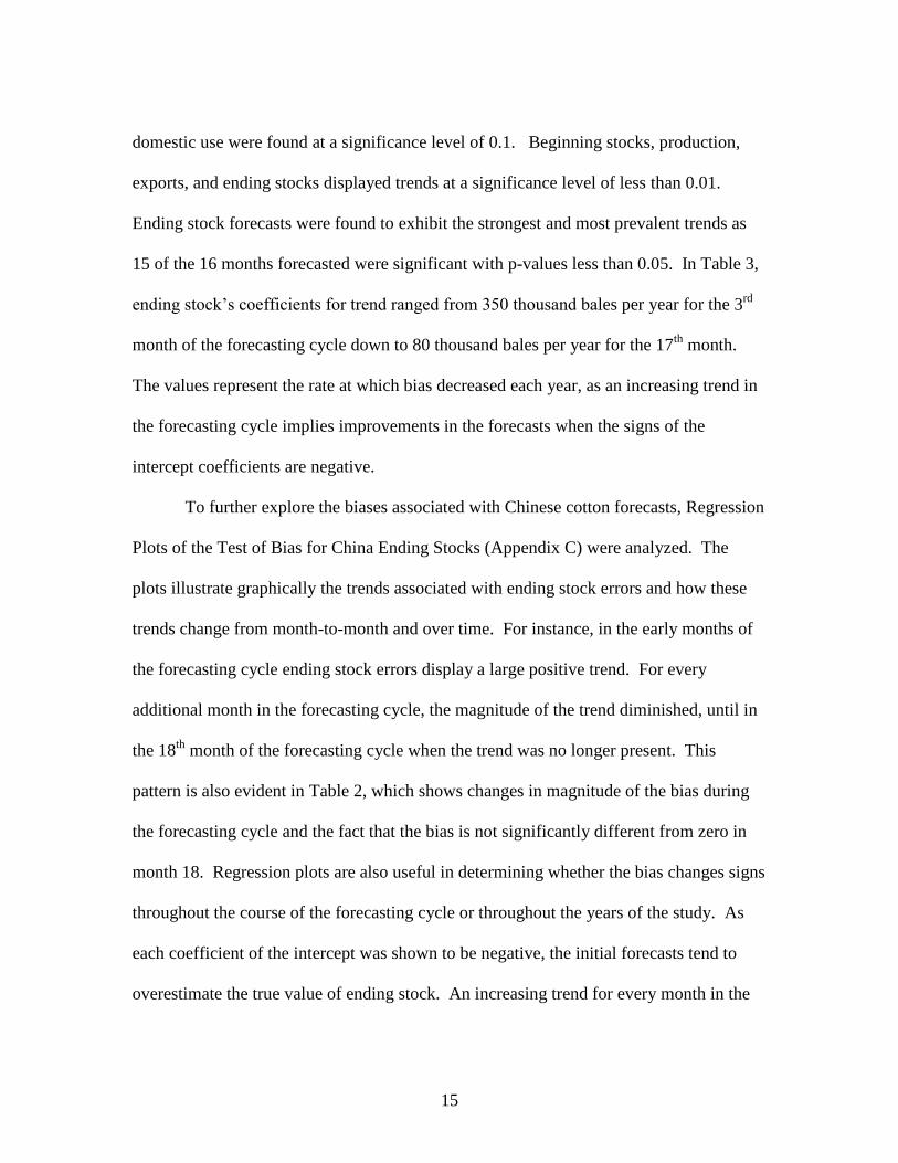
To further explore the biases associated with Chinese cotton forecasts, Regression

Plots of the Test of Bias for China Ending Stocks (Appendix C) were analyzed. The

plots illustrate graphically the trends associated with ending stock errors and how these

trends change from month-to-month and over time. For instance, in the early months of

the forecasting cycle ending stock errors display a large positive trend. For every

additional month in the forecasting cycle, the magnitude of the trend diminished, until in

the 18th

month of the forecasting cycle when the trend was no longer present. This

pattern is also evident in Table 2, which shows changes in magnitude of the bias during

the forecasting cycle and the fact that the bias is not significantly different from zero in

month 18. Regression plots are also useful in determining whether the bias changes signs

throughout the course of the forecasting cycle or throughout the years of the study. As

each coefficient of the intercept was shown to be negative, the initial forecasts tend to

overestimate the true value of ending stock. An increasing trend for every month in the

16

forecasting cycle implies that throughout the years since the 1984/85 marketing year

there have been improvements in the forecasts, as the signs of the intercept and trend are

opposite. However, the values also indicate that over time bias decreases and can quite

possibly change signs. For instance, ending stock’s 3rd

forecast has an initial bias of -

3.42. The negative bias means that in the early years 1985/86 through 1993/94, the

USDA forecasts overestimated ending stocks. The coefficient of trend for ending stocks

is 0.35 and positive, thus later forecasts 1994/95 through 2008/09 the trend overcomes

the initial bias and therefore changes the sign from negative to positive in these years.

Therefore the latest forecasts for ending stocks the USDA underestimated, which

provides further evidence that bias is dynamic and changes over time. As a result, any

adjustments must consider both components, coefficients of bias and coefficients of

trend.

WASDE World Cotton bias and trends for forecast errors are displayed in Table

4. The World cotton market contains three categories that exhibit a significant initial

bias. Domestic use and ending stocks show an initial bias at a significance level of 0.1,

while imports were found to have an initial bias at a significance level of 0.05. The table

clearly shows that the initial biases found in the imports category are the most prevalent

of all the categories in WASDE World cotton forecasts. For the first 12 months of the

forecasting cycle for World cotton imports, the forecasts were found to be significantly

underestimating cotton imports (p < 0.05). In fact, the initial bias for the first two

months of the forecasting cycle was an underestimation of more than 2.5 million bales,

though by the 12th

month the initial bias had reduced to an underestimation of around 720

17

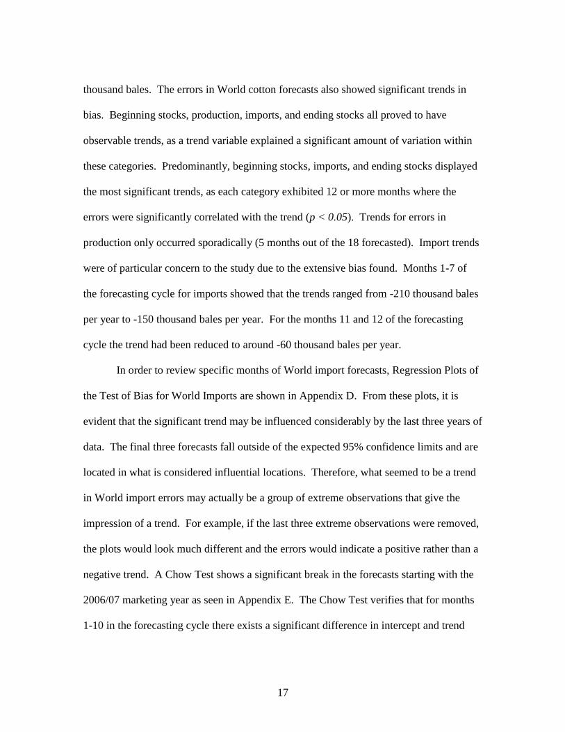
thousand bales. The errors in World cotton forecasts also showed significant trends in

bias. Beginning stocks, production, imports, and ending stocks all proved to have

observable trends, as a trend variable explained a significant amount of variation within

these categories. Predominantly, beginning stocks, imports, and ending stocks displayed

the most significant trends, as each category exhibited 12 or more months where the

errors were significantly correlated with the trend (p < 0.05). Trends for errors in

production only occurred sporadically (5 months out of the 18 forecasted). Import trends

were of particular concern to the study due to the extensive bias found. Months 1-7 of

the forecasting cycle for imports showed that the trends ranged from -210 thousand bales

per year to -150 thousand bales per year. For the months 11 and 12 of the forecasting

cycle the trend had been reduced to around -60 thousand bales per year.

In order to review specific months of World import forecasts, Regression Plots of

the Test of Bias for World Imports are shown in Appendix D. From these plots, it is

evident that the significant trend may be influenced considerably by the last three years of

data. The final three forecasts fall outside of the expected 95% confidence limits and are

located in what is considered influential locations. Therefore, what seemed to be a trend

in World import errors may actually be a group of extreme observations that give the

impression of a trend. For example, if the last three extreme observations were removed,

the plots would look much different and the errors would indicate a positive rather than a

negative trend. A Chow Test shows a significant break in the forecasts starting with the

2006/07 marketing year as seen in Appendix E. The Chow Test verifies that for months

1-10 in the forecasting cycle there exists a significant difference in intercept and trend

18

when the year is 2006 or later. This implies that the last three observations are not

consistent in trend with the prior observations. This difference in relationship should be

taken into account in any possible adjustments for bias in these forecasts.

Table 5 shows the results of the test of orthogonality (equation 4) for US cotton

forecasts. This test evaluates whether forecast errors are correlated with forecast levels,

as explained in the Methods section. The null hypothesis of an efficient forecast is

Ho:β=0, which indicates no correlation between forecast errors and forecast levels.

When β > 0, large forecast values are associated with large positive errors

(underestimation). However, when β < 0, large forecast values are associated with large

negative errors (overestimation). Results shown in Table 5 indicate that orthogonality in

US cotton forecasts was violated in only a few cases: significant positive correlation

between forecast values and forecast errors was found in months 10-11 for production

forecasts and in months 14-17 for export forecasts; significant negative correlation

between forecast values and forecast errors was found in months 13 through 15 for

ending stock forecasts. For production forecasts, the value of the β coefficient was 0.02,

thus for each additional 1 million bales forecasted there was, on average, an increase of

20 thousand bales in error. On the other hand, ending stock’s β coefficient value of -0.10,

indicates that for each additional 1 million bales forecasted there was, on average, a

decrease in the value of error by 100 thousand bales. It is important to keep in mind that

when error is already less than zero (yiT y

it < 0), the decrease in error represents an

increase in the overestimation of ending stocks. In all three categories, the inefficiencies

were found late in the forecasting cycle, generally when forecast errors were fairly small.

19

Table 6 displays the results of the test of orthogonality for WASDE forecasts for

China. Forecast errors for production, imports, domestic use, exports, and ending stocks

were all found to exhibit significant correlation with forecast levels (p < 0.05). The

categories of production and exports had β coefficients greater than zero whereas

imports, domestic use, and ending stocks had β coefficients less than zero. Specifically,

production forecast values exhibited significant positive correlation with forecast errors

for months 12-17, while export forecast values exhibited significant positive correlation

with forecast errors during months 9-16. Significant negative correlation with forecast

errors was found during months 2-9 for forecasted values of imports and domestic use,

while ending stock forecast values exhibited significant negative correlation in months 3-

8. Import forecasts were of upmost concern in Chinese cotton forecasts, as Table 6

showed that β coefficients for the imports category had the largest values and the most

months significant of all the Chinese forecast categories. For instance, imports during

months 3-10 had β coefficient values that range from -0.32 to -0.10, the values represent

that for an additional 1 million bales forecasted in the imports category, the average

decrease in error was approximately 320 thousand bales to 100 thousand bales. β

coefficients for production were relatively smaller than imports and ranged from 0.10 to

0.06 indicating an increase in production forecast errors of 100 to 60 thousand bales in

months 12-17, when an additional 1 million bales were forecasted. The values for the β

coefficients in exports ranged from 0.28 to 0.10 while domestic use β coefficients ranged

from -0.10 to -0.05. Ending stocks displayed β coefficients with larger values (-0.36 to -

0.22), however, the level of significance was less than the other categories (p < 0.1). As a

20

result, WASDE Chinese cotton forecasts are not efficient when the tests of orthogonality

yield significant β coefficients that display correlation with forecast levels.

The test of orthogonality in Table 7 displays several significant β coefficients with

respect to WASDE World cotton forecast categories (p < 0.05). Imports, domestic use,

and exports exhibited negative β coefficients, whereas beginning stock, production, and

ending stocks exhibited positive β coefficients. Most notably, β coefficients for World

imports were the strongest in magnitude and the most prevalent. As Table 7 shows β

coefficients for imports in months 1-4 indicate there was a 310-270 thousand bale

decrease in errors when an additional 1 million bales were forecasted. For month 14 of

imports the β coefficient had been reduced to 60 thousand bales per 1 million forecasted.

In domestic use forecasts, β coefficients ranged from -0.15 to -0.07 in months 1-9 and

exports showed β coefficients in months 1-4 ranged from -0.24 to -0.19. For the

production category the β coefficient values ranged from 0.18 to 0.02, for months 4-17

throughout the forecasting cycle, whereas beginning stock showed significant β

coefficients only for months 4 and 5 at values of 0.10 and 0.11, respectively. Thus β

coefficients change throughout the forecasting cycle and imply that the forecasts for

World imports are not optimal. Therefore the objective of our learning framework will be

to make adjustments such that import forecasts will be improved.

Another condition for forecast efficiency is that forecast errors must be

independent of prior errors as specified in equation (5). US, China, and World forecast

errors were evaluated in Tables 8-10. Table 8 shows the results from the test of

independence of lagged errors for US cotton forecasts. Domestic use forecast errors

21

exhibited significant positive correlation with lagged errors for months 1-6 of the

forecasting cycle (p < 0.05) whereas, exports displayed significant positive correlation in

months 16-17 of the forecasting cycle (p < 0.1). Domestic use represented the primary

concern for US cotton forecast categories as the first six months in the forecasting cycle

were found to have the largest values of β coefficients that were significantly different

than zero at p < 0.05. In particular, the 4th

month of the forecasting cycle for US

domestic use was shown to have the largest β coefficient at 0.55. As positive correlation

describes the consistency in errors, the value for the β coefficient implies that if this

year’s forecast error is increased 1 million bales, then the value for next year’s error is

expected to increase 550 thousand bales. Consequently, the error terms for domestic use

forecasts are not independent of one another, as the first six months show that the current

year’s error is correlated with the previous year’s error. Hence specific adjustments were

investigated to improve the forecasting performance of domestic use based upon these

criteria.

WASDE cotton forecasts for China were explored in Table 9 to examine whether

the categories within the Chinese forecasts exhibited any significant correlation with

lagged errors. The four categories of production, domestic use, exports, and ending stocks

had significant correlation with lagged errors at p < 0.05. Therefore for these categories,

the forecasted errors are not independent from year to year. Particularly, the domestic

use category in 10 of the 18 forecasted months exhibit significant correlation with lagged

error. The largest coefficient in magnitude is the 3rd

forecasting month of July with a

value 0.86. This value indicates that if the current year forecast error is increased 1

22

million bales the expected value for next year’s forecast error will increase 860 thousand

bales. Results in later months (12-16) show that the coefficient changes from positive to

negative. This means in months 12-16, an increase in forecast error results in a decrease

in error for the subsequent year. Specifically, for a 1 million bale increase in error, the

next year’s forecast error is expected to decrease 520 thousand to 570 thousand bales.

Conversely, if error decreases then the following year’s error is expected to increase.

Considering these coefficients, the early months of the forecasting cycle show there was a

positive correlation between lagged errors and current errors, however for later months of

the forecasting cycle, the correlation was negative. Thus the trends are dynamic

throughout the forecasting cycle. Therefore, in order for the USDA to improve

forecasting efficiency, adjustments for equation (5) must describe the relationship

between previous year’s errors and the current year’s errors.

Results from Table 10 show that lagged errors in domestic use forecasts are the

primary concern in the evaluation of World cotton forecasts. Domestic use forecasts

exhibited similar patterns as what was found in the evaluation of U.S. and Chinese

markets. Domestic use errors were shown to be higher correlated with lagged errors than

other forecast categories. Specifically, domestic use errors showed significant negative

correlation with lagged errors in months 12 through 15 (p < 0.05). In particular, month

15 displayed the largest β coefficient which showed that errors were expected to decrease

560 thousand bales in the next year when the current year error increased an additional 1

million bales, while month 12 displayed the smallest β coefficient which described that

domestic use error was expected to decrease 470 thousand bales for the next year when

23

the error increased an additional 1 million bales this year. Beginning stock and export

forecast errors were also found to exhibit significant correlation with lagged errors (p <

0.1) as evidenced in Table 10, although, only two months were significant for each

category. Beginning stocks displayed significant β coefficients for months 2 and 5 with

values of 0.36 to 0.38, respectively, whereas exports exhibited significant correlation

with lagged error in months 15 and 18 with β coefficients of 0.36 and -0.45. Thus lagged

errors were shown to contribute to variation in forecasts and forecast errors. Thus, in

order to improve forecasts, adjustments are needed to correct for the correlated errors

within the forecasting cycle.

Equation (6) in the forecast evaluation framework evaluates whether forecast

revisions are independent within a forecasting cycle. According to the results of the tests

of independence for US revisions shown in Table 11, production, domestic use, exports,

ending stocks, and price all exhibited significant correlation in forecast revisions (p <

0.1). Thus revisions are not independent of one another. In particular, domestic use

forecast revisions displayed the most prevalent and largest β coefficients of all the

categories in the evaluation. Specifically, β coefficients for revisions showed significant

positive correlation in 8 months out of the 17 months recorded which designated that

there was a positive relationship between the revisions in the forecasting cycle. For

instance, domestic use revisions for the 10th

month of the forecasting cycle exhibited the

largest β coefficient value at 1.51, which indicated that the revisions from month 9 to

month 10 were 1.51 times larger than the revisions from month 8 to month 9, on average.

In other months that were found to be significant for domestic use revisions the β

24

coefficient values were considerably less than in month 10, such that the coefficient

values ranged from 0.26 in month 9 to 0.85 in month 3. In other categories from US

cotton forecasts the correlations were not as prevalent or as strong as with domestic use,

though the β coefficients were significant. For production, the β coefficients ranged from

0.57 in month 6 reducing down to less than 0.01 in month 14. The β coefficients in US

exports ranged from 0.99 in month 6 down to 0.23 in month 17, while ending stocks

displayed β coefficients that ranged from 0.68 in month 10 down to 0.33 in month 4.

Price, on the other hand, displayed the smallest amount of correlation with forecast

revisions as only month 8 and month 16 were significant with β coefficient values of 0.34

and -0.14, respectively. Therefore, as found within Table 11, relationships between

revisions may have significant effects on forecast errors and the forecasts themselves,

hence, the relevance of the proposed learning framework.

Table 12 displays the results for the test of independence of revisions in WASDE

Chinese forecasts. The categories of production, imports, domestic use, exports and

ending stocks were all shown to exhibit significant correlation with forecast revisions.

Imports exhibited not only the strongest relationships between revisions but also

displayed the most months out of the forecasting cycle that were significant.

Specifically, 8 months were shown to exhibit p-values of less than 0.05, with month 5

displaying the largest β coefficient value at 1.61. Therefore, the revisions from month 4

to month 5 are expected to be 1.61 times larger than the revisions from month 3 to month

4. As for the production category, four months were found to have significant β

coefficients that ranged in value from 0.76 in month 5 to less than 0.01 in month 16. In

25

domestic use and exports, each category displayed 6 months in which β coefficients were

significant, where the coefficients ranged in values from 0.95 in month 10 to -1.34 in

month 17 for domestic use, and exports displayed values that ranged from 1.16 in month

16 to 0.43 in month 11. Ending stocks displayed the smallest number of significant β

coefficients as only month 9 and month 14 were significant with values of 0.62 and -0.41,

respectively. Thus, months in which significant β coefficients were displayed indicates

that the forecasts are not independent of one another. Therefore, proposed corrections

based upon the β coefficient values are identified and evaluated for China imports within

the learning framework.

Table 13, the test of independence of forecast revisions for World forecasts,

showed that every category displayed significant correlation with revisions throughout

the forecasting series. However, the domestic use category, yet again, exhibited the

highest number of months with significant correlation in forecast revisions and the

strongest β coefficients. Thus, the results from Table 13 provide even more evidence to

investigate the adjustment of domestic use forecasts. For the World cotton market,

domestic use forecasts displayed 8 months in which significant correlation was present in

forecast revisions (p < 0.05). In particular, domestic use’s largest β coefficient was found

in month 10 at a value of 1.34, which indicated that the revisions between month 9 and

month 10 were 1.34 times larger than the revisions between month 8 and month 9.

Furthermore, for the other 7 months in which revisions were found to be significantly

correlated the β coefficients ranged from 1.17 in month 6 reducing down to 0.31 in month

11. Thus, forecasts and forecast revisions are not independent of one another throughout

26

the domestic use forecasting cycle. As for the other World forecasting categories, the β

coefficients were less significant and had much smaller values than the values displayed

for domestic use. For instance, beginning stocks exhibited only one month in which

revisions were significant (month 17), and the β coefficient’s value was -0.27.

Production and imports, on the other hand, displayed 5 months and 6 months that were

respectively significant. Production had β coefficients that ranged from 0.48 in month 9

down to -0.07 in month 19, whereas β coefficients for imports ranged from 0.92 in month

6 down to 0.22 in month 12. Export and ending stock forecasts also displayed significant

correlation between revisions, as export forecasts showed 7 months that were significant

and ending stock forecasts showed 4 months that were significant. Export β coefficients

ranged from 0.76 in month 10 down to -0.18 in month 14, while ending stock β

coefficients ranged from 0.53 in month 9 and reducing down to -0.81 in month 18. Thus,

in order improve forecasts evaluated in Table 13, the study proposed a

correction/adjustment procedure based on the results of evaluation.

27

CHAPTER FOUR

LEARNING FRAMEWORK

Adjustment Procedure:

The purpose of adjusting forecasts is to reduce bias and systematic error within

USDA WASDE cotton forecasts. The end goal being a forecast that is optimal based

upon the properties/criteria defined in the evaluation framework. Adjustments were

made based on the results of the forecast evaluation only in months where significant

deviations from efficiency were found. The adjustments were performed in the following

manner: the study period (1985-2008) was split into two subsets, an evaluation subset

(starting with 1985-1998) and validation subset (1999-2008). The evaluation subset was

then used to estimate parameters for the test of bias, test of orthogonality, test of weak

form efficiency, and the test of revisions. The validation subset was used to adjust

published forecasts and evaluate whether these adjustments improved the forecasts.

Thus, for the first observation in the validation subset, the marketing year of 1999/00, the

estimation subset consisted of 1985-1998 marketing years. The second observation in the

validation subset was adjusted based on parameters calculated with 15 observations

(1985/86-2000/01) in the evaluation subset. The process was repeated until the

evaluation subset consisted of 24 observations to generate parameters used to evaluate the

last year of the validation subset (2008/09) forecasts. Thus the validation subset

consisted of 10 observations (1999/00-2008/09). The adjusted forecasts (adj yti+1

) were

calculated as follows:

28

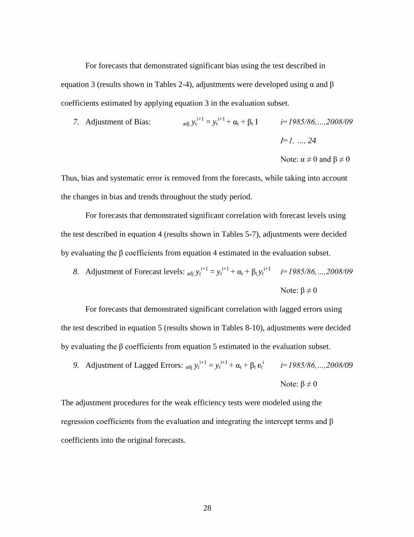
For forecasts that demonstrated significant bias using the test described in

equation 3 (results shown in Tables 2-4), adjustments were developed using α and β

coefficients estimated by applying equation 3 in the evaluation subset.

7. Adjustment of Bias: adj yti+1

= yti+1

+ αt + βt I i=1985/86,…,2008/09

I=1, …, 24

Note: α ≠ 0 and β ≠ 0

Thus, bias and systematic error is removed from the forecasts, while taking into account

the changes in bias and trends throughout the study period.

For forecasts that demonstrated significant correlation with forecast levels using

the test described in equation 4 (results shown in Tables 5-7), adjustments were decided

by evaluating the β coefficients from equation 4 estimated in the evaluation subset.

8. Adjustment of Forecast levels: adj yti+1

= yti+1

+ αt + βt yti+1

i=1985/86,…,2008/09

Note: β ≠ 0

For forecasts that demonstrated significant correlation with lagged errors using

the test described in equation 5 (results shown in Tables 8-10), adjustments were decided

by evaluating the β coefficients from equation 5 estimated in the evaluation subset.

9. Adjustment of Lagged Errors: adj yti+1

= yti+1

+ αt + βt eti i=1985/86,…,2008/09

Note: β ≠ 0

The adjustment procedures for the weak efficiency tests were modeled using the

regression coefficients from the evaluation and integrating the intercept terms and β

coefficients into the original forecasts.

29

For forecasts that demonstrated significant correlation between revisions using the

test described in equation 6 (results shown in Tables 11-13), adjustments were calculated

by evaluating the β coefficients from equation 6 estimated in the evaluation subset.

10. Adjustment of Revisions: adj yt+1i+1

= yt+1i+1

+ γt+1 rti i=1985/86,…,2008/09

t=2,…,19

Note: γ ≠ 0

Validation Measures:

Two measures that were used to compare and evaluate forecast improvements

were mean absolute error (MAE) and root mean squared error (RMSE), as defined below:

11.

and

12.

MAE estimates the average of the absolute errors between the final forecast and

the observed monthly forecasts, whereas RMSE estimates the square root of the average

squared difference between the final forecast and the observed monthly forecasts. Hence,

when both statistics are zero the monthly forecasts are perfect and estimate the final

forecast values exactly. However, when error is found in the forecasting series, MSE and

RMSE increase the larger the magnitude of the error. Both measures were calculated

because both are effective at comparing models. Specifically, MAE describes the average

magnitude of the forecast errors, whereas RMSE measures how far, on average, the

30

monthly forecasts were from the final value and is more sensitive to forecasts that have

large errors than MAE.

Validation of Adjustments:

Tables 15-26 show results from the comparison of original forecast errors and

adjusted forecast errors for the most significant categories from the forecast evaluations.

Each table shows the original errors, errors associated with adjusted forecasts, and the

difference between the two as an indication of the improvement due to the adjustments.

Table 15 shows that US domestic use forecasts adjusted for bias improve forecast

efficiency overall using MAE as a measure of error. However, using RMSE as a measure

of error determined that adjusted domestic use forecasts were less accurate than the

original. Thus adjusted forecasts for domestic use displayed forecast errors that were on

average closer to zero than the original forecasts yet exhibited forecast errors that were

also more extreme than the original forecast errors. Therefore, the averages of the

squared errors were larger, which indicates that adjustments at times over-corrected for

bias causing more extreme errors. This suggests that adjustments to US domestic use

forecasts may not be appropriate given there is no agreement between the two measures

of error. For instance, the only two months out of the forecasting cycle that were shown

to have improved MAE and RMSE values were the 5th

and 6th

months of the forecasting

cycle, September and October. Though, the improvements were relatively small at 40

thousand bales for both months using MAE as a measure of error and 20 to 30 thousand

31

bales using RMSE as a measure of error. Consequently, it is questionable whether

forecast adjustments would improve US domestic use forecast efficiency.

Evaluation for the adjustment of bias in Chinese ending stocks is displayed in

Table 16. The improvement in forecast errors is obvious as adjusted forecasts were

shown to improve both MAE and RMSE overall. Evidence shows that in 12 months out

of the 15 months adjusted, improvements were made in MAE and RMSE. For MAE the

largest improvements were early in the forecasting cycle at 750 thousand bales and 980

thousand bales, on average, for months 3 and 4 of the forecasting cycle. Improvements

were also evident in month 5 and months 8-16 ranging from 710 thousand bales to 160

thousand bales, on average. The RMSE column displays similar positive results from the

evaluation of the adjustment of bias suggesting that not only the mean, but also

variability of forecasts were improved due to adjustment. The largest improvements in

RMSE occurred in months 4 and 5 of the forecasting cycle at 1.18 and 1.03 million bales,

while the improvements in months 3 and months 8-17 ranged from 170 to 840 thousand

bales. This leads us to believe that China ending stocks could benefit substantially from

adjustments based upon the Dynamic Test of Bias.

For the world, the Dynamic Test of Bias evaluation model was ineffective at

producing adjustments that actually benefit import forecasts. Table 17 shows that MAE

and RMSE were smaller, overall, before the adjustments were made. In particular, there

was only two months in which both MAE and RMSE actually improved from the forecast

adjustments (month 7 & 16). The improvement, measured as MAE, was 200 thousand

bales in month 7 and 10 thousand bales in month 16. Likewise, the improvement,

32

measured as RMSE, was 30 thousand bales in month 7 and 10 thousand bales in month

16. Additional improvements were realized in in terms of MAE during months 6, 8, 9

which ranged from 230 thousands bales in month 8 to 80 thousand bales in month 9.

However, the overall difference in original forecast error and adjusted forecast error was

negative for both measures of error, MAE and RMSE, which indicated that the adjusted

forecasts were not improvements to the original forecasts but actually a loss in quality.

The evaluation for the adjustment of forecast levels, Tables 18-20, proved that

forecast adjustments based on the test of orthogonality were ineffective in producing

more efficient forecasts for the regions of US, China, and the World. Specifically, Table

18 does not display any improvements at all in US production forecasts. Neither measure

of error, MAE or RMSE, was improved by allowing adjustments to the original

production forecasts, as there was not a single month in which adjusted forecasts

provided any benefits to the US production forecasting cycle. Interestingly, there was not

a single month that displayed a significant decrease or increase in forecast error for

production, as every month in which forecasts were adjusted displayed zero as the

difference between the original and adjusted forecast errors, for both MAE and RMSE.

This implies that the relationship detected between forecast levels and forecast errors in

US production was not strong enough in magnitude to yield significantly different

forecast errors/forecasts when the forecast adjustments were applied.

Table 19 displays the results from the evaluation for the adjustment of forecast

levels in Chinese import forecasts. As mentioned previously, the test of orthogonality

was ineffective at producing adjusted forecasts that were more efficient than the original

33

forecasts. Thus, there was no overall improvement in MAE or RMSE in Chinese import

forecasts. In fact, the import forecast errors were greater, on average, for every month in

which adjustments were included. The difference in errors for MAE seemed to be the

largest around month 5 at 340 thousand bales and was the smallest during month 3 at 80

thousand bales. The increased errors in RMSE were the largest in magnitude for the early

months of the forecasting cycle (months 3-5) where values reached 1.25 million bales,

and reduced down to 240 thousand bales for month 13. Therefore, the adjustments for

forecast levels did not provide any value to Chinese import forecasting.

In Table 20, adjustments of forecast levels for World import forecasts were found

to increase forecast errors in terms of MAE and RMSE. In fact, only 4 months out of the

14 months adjusted were errors smaller as measured by MAE, such that month 1 saw a

decrease in error of 10 thousand bales and months 6-9 saw a decrease in errors of 30 to

60 thousand bales. Particularly, there were no months found in which both measures,

MAE and RMSE improved due to the adjustments of forecast levels. For RMSE, every

month that was adjusted, the forecast errors increased, on average, ranging from 20

thousand bales in month 1 up to 440 thousand bales in month 12. Thus, overall, the

forecast errors were not any smaller than what was found for the original forecasts.

Tables 21-23 represent the evaluation of the adjustments for the weak efficiency

criteria described in equation (5). For US domestic use forecasts, the evaluation for the

adjustments of lagged errors are shown in Table 21. The results describe that when

domestic use forecasts were adjusted for lagged errors, overall improvement was found in

terms of MAE, but not RMSE. This implies that absolute error for the US domestic use

34

forecasts decreased on average when the forecasts were adjusted but squared forecast

error, on average, was found to remain about the same or larger than the original

forecasts. Thus, there is indication that there may be additional error associated with

extreme values when evaluating error using RMSE. In particular, improvement in terms

of MAE was shown in months 2-6, ranging from 10 thousand bales in month 2 up to 70

thousand bales in month 3. As for improvement in RMSE, only months 4 and 5 showed

positive values for the difference in error of original forecasts and adjusted forecasts, the

values for the improvement in terms of RMSE were 30 thousand bales and 20 thousand

bales, respectively. Therefore, the errors in US domestic use forecasts were improved in

some cases by using adjustments for lagged errors, although the improvement overall was

small relative to the error from the original forecasts. Specifically, MAE saw the most

improvement overall (150 thousand bales) while RMSE displayed no difference in

original forecast errors and adjusted forecast errors.

Adjustments made to Chinese domestic use forecasts were evaluated in Table 22.

The forecasts showed overall improvement in both MAE and RMSE. Specifically, 6

months out of the 11 months adjusted showed improvement in terms of both MAE and

RMSE (months 3-7, 15). The most improvement for MAE was found early in the

forecasting cycle during months 3-6 and ranged in values from 510 to 560 thousand

bales, while later in the forecasting cycle (month 15) improvement was reduced down to

40 thousand bales. Similarly for RMSE, the greatest improvement was found in months

3-6, ranging in values from 510 thousand bales in month 3 down to 260 thousand bales in

month 6. Adjustments for months 7, 15, 16 also showed improvements in RMSE,

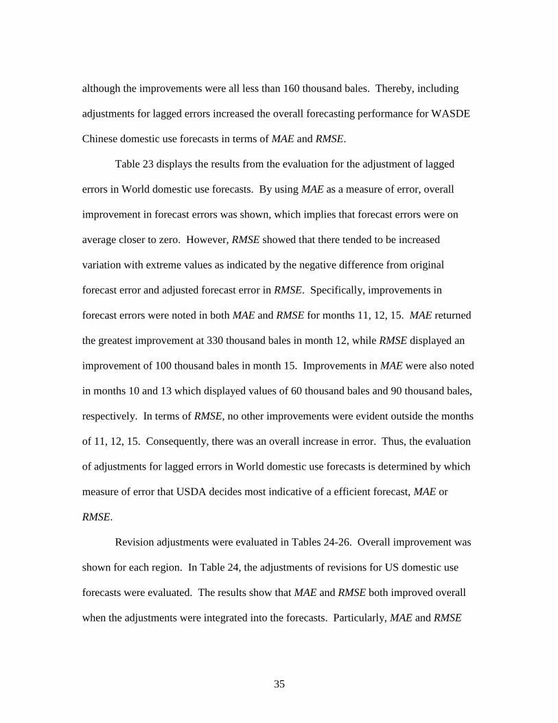
35

although the improvements were all less than 160 thousand bales. Thereby, including

adjustments for lagged errors increased the overall forecasting performance for WASDE

Chinese domestic use forecasts in terms of MAE and RMSE.

Table 23 displays the results from the evaluation for the adjustment of lagged

errors in World domestic use forecasts. By using MAE as a measure of error, overall

improvement in forecast errors was shown, which implies that forecast errors were on

average closer to zero. However, RMSE showed that there tended to be increased

variation with extreme values as indicated by the negative difference from original

forecast error and adjusted forecast error in RMSE. Specifically, improvements in

forecast errors were noted in both MAE and RMSE for months 11, 12, 15. MAE returned

the greatest improvement at 330 thousand bales in month 12, while RMSE displayed an

improvement of 100 thousand bales in month 15. Improvements in MAE were also noted

in months 10 and 13 which displayed values of 60 thousand bales and 90 thousand bales,

respectively. In terms of RMSE, no other improvements were evident outside the months

of 11, 12, 15. Consequently, there was an overall increase in error. Thus, the evaluation

of adjustments for lagged errors in World domestic use forecasts is determined by which

measure of error that USDA decides most indicative of a efficient forecast, MAE or

RMSE.

Revision adjustments were evaluated in Tables 24-26. Overall improvement was

shown for each region. In Table 24, the adjustments of revisions for US domestic use

forecasts were evaluated. The results show that MAE and RMSE both improved overall

when the adjustments were integrated into the forecasts. Particularly, MAE and RMSE

36

both showed decreases in forecast error for 7 months out of the 11 adjusted.

Improvements in MAE ranged from 40 thousand bales in month 3 down to less than 10

thousand bales for month 13. Improvements in RMSE ranged from 30 thousand bales in

month 3 down to less than 10 thousand bales in month 10. Interestingly, both MAE and

RMSE saw the most improvement early on, as adjustments for revisions in the 3rd

month

of the forecasting cycle returned the greatest decrease in forecast error. Thus, there is

reason to believe that revision adjustments might be beneficial for future forecasts as

well. Although, most revision adjustments were found to be relatively small in

comparison to the forecasted values, the adjustments did provide overall improvement, in

terms of MAE and RMSE. As a result, US domestic use forecasts could benefit if the

adjustment procedure were adopted.

Adjustments of revisions for Chinese import forecasts were evaluated in Table 25.

The results show that overall improvement was found in terms of MAE and RMSE. MAE

improved for 7 months out of the 8 months adjusted, while RMSE improved in every

month adjusted. The improvement in MAE ranged from 10 thousand bales in month 9 up

to 380 in month 7, whereas improvement in RMSE ranged from 10 thousand bales in

month 10 up to 490 thousand bales in month 7. Thus, substantial improvements in

forecast errors were evidenced when Chinese import forecasts were adjusted for

revisions. Particularly, in terms of RMSE, which tends to amplify errors associated with

extreme observations, the improvements were the greatest. Therefore, revision

adjustments may significantly reduce forecast errors and improve the forecasting

performance for Chinese imports.

37

Table 26 displays the results from the evaluation for the adjustment of revisions in

World domestic use forecasts. In terms of both MAE and RMSE, overall improvement in

forecast errors was shown, which implies that forecast errors were, on average, not only

closer to zero, but squared errors were improved as well. Specifically, the results showed

that of the 8 months adjusted, 6 months displayed considerable improvement in terms of

MAE and RMSE. For MAE, months 4-6 and months 8-10 showed that forecast errors

decreased on average from 30 thousand bales in month 4 up to 160 thousand bales in

month 10. In terms of RMSE, the same six months were found to exhibit improvements,

where month 8 displayed the largest improvement at 310 thousand bales and month 4

displayed the smallest improvement at 70 thousand bales. Thus forecast errors in terms

of MAE and RMSE decreased during the same months and exhibited similar

improvements. Therefore, the adjustments of revisions for World domestic use forecasts

provided valuable improvements to the original forecasts.

38

CHAPTER FIVE

SUMMARY AND CONCLUSIONS

This study applied an evaluation framework to test the efficiency of USDA

WASDE cotton forecasts. The framework provided useful insight into the errors

associated with forecasting WASDE cotton categories. Adjustment procedures were

designed to correct for the inefficiencies found within the WASDE forecasts. The

corrections or ―adjustments‖ were validated, by comparing the errors from adjusted

forecasts to the errors from the original forecasts, thus providing evidence to confirm the

benefits of adjustment.

The findings from the study show that some forecasts from the US, China, and the

World, suffer from inefficiencies defined in the forecast evaluation framework. In

particular, domestic use forecasts displayed the most problems among the US cotton

forecast categories. Table 14 illustrates that domestic use displayed significant β

coefficients for the test of bias, the test of weak efficiency, and the test of revisions.

Thus, indicating that domestic use forecasts may benefit from forecast adjustments. US

domestic use forecast adjustments were evaluated in Tables 15, 21, 24. The results

describe that the adjustments of bias and the adjustments of lagged errors provided

improvement to forecasts with a 2% reduction in MAE and a 4% reduction in RMSE.

Though, RMSE was found to remain the same for the test of bias and the test of weak

efficiency. The test of revisions showed the most positive results from the adjustment

procedure as both MAE and RMSE improved. MAE displayed a 2% reduction as a result

39

of the adjustment of revisions, while RMSE displayed a 1% reduction as a result of the

adjustment of revisions.

Chinese ending stock forecasts displayed the most substantial improvement of all

the adjusted forecasts. Particularly, in terms of the adjustment for bias, there was

approximately a 20% reduction in MAE and a 20% reduction in RMSE due to the forecast

adjustments. The adjustments made based upon the test of orthogonality showed the least

improvement to cotton forecasts for China as neither MAE nor RMSE improved.

However, for domestic use forecasts the adjustments for lagged errors showed

considerable improvement in MAE and RMSE at 9% and 7%, respectively. Adjustment

of revisions for Chinese import forecasts also indicated a substantial improvement in

MAE and RMSE, as MAE was shown to be reduced by 6% due to the adjustments made in

forecasts, while RMSE was reduced by 7% due to the adjustments made in forecasts.

Thus, forecast adjustments were found to be very beneficial for WASDE Chinese cotton

forecast categories.

World forecast evaluations followed similar patterns as found in US forecast

adjustments. This implies that for the World forecasts, imports and domestic use were

the primary categories that displayed deviations from efficiency. As for the evaluation of

forecast adjustments, the World forecasts were extremely different than Chinese

forecasts. In particular, the adjustment for bias and the adjustment for forecast levels

provided no benefit to World import forecasts. However, for domestic use forecasts, the

adjustment for lagged errors provided a considerable benefit to MAE with approximately

a 3% reduction, although, RMSE was shown to increase as a result of additional error.

40

The adjustment of revisions provided the most consistent improvement in World forecast

errors as domestic use forecasts were adjusted such that both MAE and RMSE were

improved. MAE was reduced by 2% due to forecast adjustments in domestic use, while

RMSE was reduced by 3% due to the forecast adjustments. Therefore, World forecast

categories were shown to benefit from the adjustments of lagged errors and the

adjustments of revisions.

Overall, the evaluation and the adjustment of forecasts provided a framework to

study and improve forecasting techniques. The results from the study suggest that every

region would benefit from an adjustment procedure. In particular, Chinese cotton

forecasts would benefit most of all, as Chinese forecasts tended to express significant bias

and trends that increased forecast errors. The framework developed in the study will

provide the USDA a valuable opportunity to reduce and improve forecast accuracy and

efficiency.

In conclusion, there are plenty more opportunities for future researchers in the

evaluation of USDA WASDE cotton forecasts, such as: 1) Investigation of correlation of

errors between forecast categories. 2) Research different functional forms of the

equations in the evaluation framework. 3) Develop a new test statistic or formal

hypothesis test, in order to test whether forecast errors are significantly less than original

forecast errors. 4) Develop an adaptive adjustment procedure that adjusts forecasts

dynamically according to evaluation subset.

Table 1. USDA WASDE Forecast Evaluation Summary for 1985-2008 Marketing Years:

Most Significant Categories found within the Forecasting Evaluation Framework (By Region)

Category Beginning Stocks

(M.Bal)

Production

(M.Bal)

Imports

(M.Bal)

Domestic Use

(M.Bal)

Exports

(M.Bal)

Ending Stocks

(M.Bal)

Price

(¢/lb)

World Mean 40.90 92.42 28.80 93.23 28.46 40.58 N/A

Std Deviation 10.61 14.50 5.35 13.22 5.82 10.87 N/A

Coeff Variation (percent) 25.95 15.69 18.58 14.18 20.45 26.80 N/A

Skewness 0.77 0.92 1.31 1.20 1.39 0.70 N/A

Kurtosis 0.02 0.03 1.81 0.53 1.97 -0.29 N/A

China Mean 13.14 22.94 3.72 26.79 0.76 12.56 N/A

Std Deviation 5.15 6.01 4.76 10.63 0.90 4.85 N/A

Coeff Variation (percent) 39.20 26.22 127.89 39.69 118.74 38.65 N/A

Skewness -0.10 1.43 1.92 1.42 1.50 -0.11 N/A

Kurtosis -0.93 1.19 3.94 0.63 1.53 -0.92 N/A

US Mean N/A 17.12 N/A 8.22 8.92 5.22 55.82

Std Deviation N/A 3.41 N/A 2.27 3.84 2.20 10.71

Coeff Variation (percent) N/A 19.89 N/A 27.61 43.04 42.21 19.19

Skewness N/A -0.01 N/A -0.35 0.63 0.84 -0.29

Kurtosis N/A 0.07 N/A -0.87 -0.09 -0.03 0.12

Note: N=24 years * Denotes significance level of 0.1 ** Denotes significance level of 0.05 *** Denotes significance level of 0.01

41

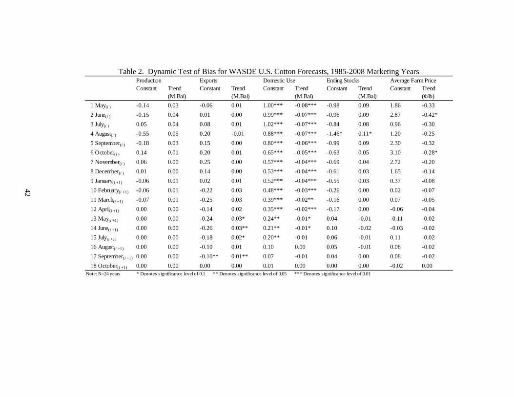
Table 2. Dynamic Test of Bias for WASDE U.S. Cotton Forecasts, 1985-2008 Marketing Years

Constant Trend

(M.Bal)

Constant Trend

(M.Bal)

Constant Trend

(M.Bal)

Constant Trend

(M.Bal)

Constant Trend

(¢/lb)

1 May(i ) -0.14 0.03 -0.06 0.01 1.00*** -0.08*** -0.98 0.09 1.86 -0.33

2 June(i ) -0.15 0.04 0.01 0.00 0.99*** -0.07*** -0.96 0.09 2.87 -0.42*

3 July(i ) 0.05 0.04 0.08 0.01 1.02*** -0.07*** -0.84 0.08 0.96 -0.30

4 August(i ) -0.55 0.05 0.20 -0.01 0.88*** -0.07*** -1.46* 0.11* 1.20 -0.25

5 September(i ) -0.18 0.03 0.15 0.00 0.80*** -0.06*** -0.99 0.09 2.30 -0.32

6 October(i ) 0.14 0.01 0.20 0.01 0.65*** -0.05*** -0.63 0.05 3.10 -0.28*

7 November(i ) 0.06 0.00 0.25 0.00 0.57*** -0.04*** -0.69 0.04 2.72 -0.20

8 December(i ) 0.01 0.00 0.14 0.00 0.53*** -0.04*** -0.61 0.03 1.65 -0.14

9 January(i +1) -0.06 0.01 0.02 0.01 0.52*** -0.04*** -0.55 0.03 0.37 -0.08

10 February(i +1) -0.06 0.01 -0.22 0.03 0.48*** -0.03*** -0.26 0.00 0.02 -0.07

11 March(i +1) -0.07 0.01 -0.25 0.03 0.39*** -0.02** -0.16 0.00 0.07 -0.05

12 April(i +1) 0.00 0.00 -0.14 0.02 0.35*** -0.02*** -0.17 0.00 -0.06 -0.04

13 May(i +1) 0.00 0.00 -0.24 0.03* 0.24** -0.01* 0.04 -0.01 -0.11 -0.02

14 June(i +1) 0.00 0.00 -0.26 0.03** 0.21** -0.01* 0.10 -0.02 -0.03 -0.02

15 July(i +1) 0.00 0.00 -0.18 0.02* 0.20** -0.01 0.06 -0.01 0.11 -0.02

16 August(i +1) 0.00 0.00 -0.10 0.01 0.10 0.00 0.05 -0.01 0.08 -0.02

17 September(i +1) 0.00 0.00 -0.10** 0.01** 0.07 -0.01 0.04 0.00 0.08 -0.02

18 October(i +1) 0.00 0.00 0.00 0.00 0.01 0.00 0.00 0.00 -0.02 0.00

Note: N=24 years * Denotes significance level of 0.1 ** Denotes significance level of 0.05 *** Denotes significance level of 0.01

Production Exports Domestic Use Ending Stocks Average Farm Price

42

Table 3. Dynamic Test of Bias for WASDE China Cotton Forecasts, 1985-2008 Marketing Years

Constant Trend

(M.Bal)

Constant Trend

(M.Bal)

Constant Trend

(M.Bal)

Constant Trend

(M.Bal)

Constant Trend

(M.Bal)

Constant Trend

(M.Bal)

1 May(i )

2 June(i )

3 July(i ) -1.81* 0.22*** -2.34* 0.21** 1.64 -0.14 1.04 -0.06 0.13 -0.02 -3.42** 0.35***

4 August(i ) -2.01** 0.23*** -2.12* 0.20** 1.63 -0.13 1.09 -0.07 0.16 -0.02 -3.47** 0.35***

5 September(i ) -1.68* 0.21*** -1.84 0.20** 1.46 -0.12 0.96 -0.05 0.15 -0.01 -2.96** 0.33***

6 October(i ) -1.46* 0.16** -1.80 0.17** 1.39 -0.11 1.02 -0.05 0.15 -0.01 -3.10** 0.30***

7 November(i ) -1.24 0.15** -1.10 0.14** 1.35 -0.11* 0.89 -0.05 0.19 -0.02 -2.11 0.24**

8 December(i ) -1.16 0.14** -0.83 0.12** 1.18 -0.10* 0.85 -0.04 0.21 -0.02 -1.89 0.22**

9 January(i +1) -1.12 0.14** -0.77 0.11** 0.91 -0.07 0.85 -0.04 0.25 -0.02 -2.10* 0.24***

10 February(i +1) -0.98 0.12** -0.42 0.08 0.68 -0.05 0.83 -0.03 0.24 -0.02 -1.82* 0.20***

11 March(i +1) -0.98 0.13** -1.13* 0.12*** 0.54 -0.05 0.66 -0.02 0.21 -0.01 -2.47** 0.24***

12 April(i +1) -1.05 0.12** -0.40 0.07** 0.48 -0.04 0.12 0.01 0.22 -0.01 -1.36** 0.15***

13 May(i +1) -0.65 0.08** -0.34 0.06** 0.33 -0.03 0.04 0.01 0.24 -0.01 -1.05* 0.12***

14 June(i +1) -0.60 0.08** -0.47 0.06** 0.12 -0.01 0.00 0.01 0.27** -0.02** -1.33*** 0.15***

15 July(i +1) -0.15 0.02 -0.36 0.05** 0.10 -0.01 0.18 -0.01 0.25*** -0.01** -0.91** 0.10***

16 August(i +1) -0.21 0.03* -0.36 0.05** 0.03 0.00 0.24 -0.01 0.14*** -0.01** -0.99** 0.10***

17 September(i +1) -0.21 0.03* -0.26 0.03* 0.04 0.00 0.33 -0.03* -0.02 0.00 -0.64 0.08**

18 October(i +1) -0.04 0.01 0.00 0.00 0.01 0.00 0.20 -0.01 0.00 0.00 -0.23 0.02

Note: N=24 years * Denotes significance level of 0.1 ** Denotes significance level of 0.05 *** Denotes significance level of 0.01

Production Imports Exports Ending StocksDomestic UseBeginning Stock

43

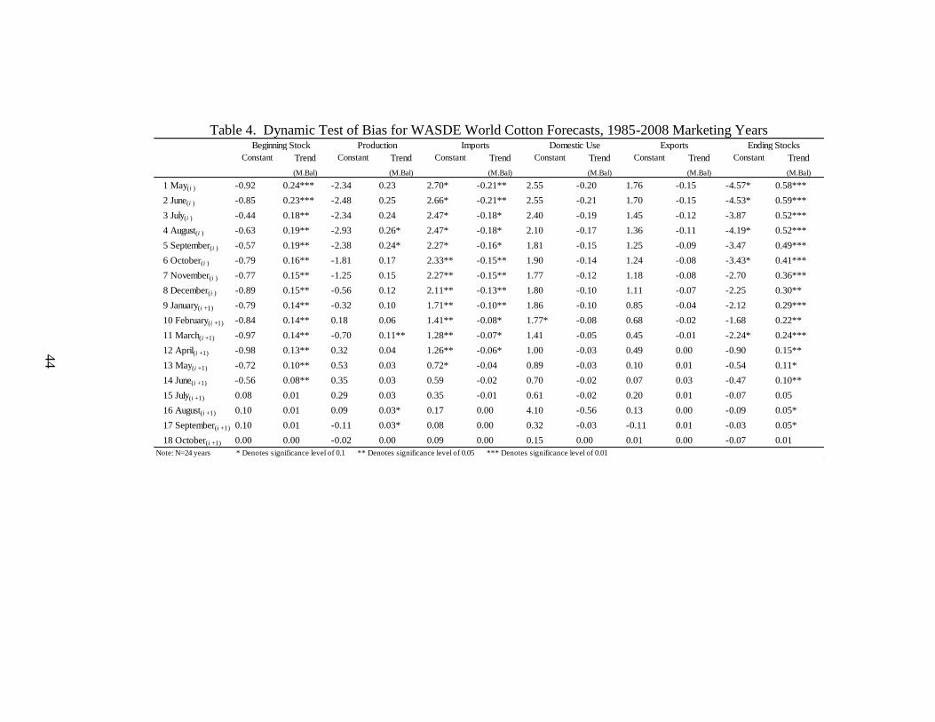
Table 4. Dynamic Test of Bias for WASDE World Cotton Forecasts, 1985-2008 Marketing Years

Constant Trend

(M.Bal)

Constant Trend

(M.Bal)

Constant Trend

(M.Bal)

Constant Trend

(M.Bal)

Constant Trend

(M.Bal)

Constant Trend

(M.Bal)

1 May(i ) -0.92 0.24*** -2.34 0.23 2.70* -0.21** 2.55 -0.20 1.76 -0.15 -4.57* 0.58***

2 June(i ) -0.85 0.23*** -2.48 0.25 2.66* -0.21** 2.55 -0.21 1.70 -0.15 -4.53* 0.59***

3 July(i ) -0.44 0.18** -2.34 0.24 2.47* -0.18* 2.40 -0.19 1.45 -0.12 -3.87 0.52***

4 August(i ) -0.63 0.19** -2.93 0.26* 2.47* -0.18* 2.10 -0.17 1.36 -0.11 -4.19* 0.52***

5 September(i ) -0.57 0.19** -2.38 0.24* 2.27* -0.16* 1.81 -0.15 1.25 -0.09 -3.47 0.49***

6 October(i ) -0.79 0.16** -1.81 0.17 2.33** -0.15** 1.90 -0.14 1.24 -0.08 -3.43* 0.41***

7 November(i ) -0.77 0.15** -1.25 0.15 2.27** -0.15** 1.77 -0.12 1.18 -0.08 -2.70 0.36***

8 December(i ) -0.89 0.15** -0.56 0.12 2.11** -0.13** 1.80 -0.10 1.11 -0.07 -2.25 0.30**

9 January(i +1) -0.79 0.14** -0.32 0.10 1.71** -0.10** 1.86 -0.10 0.85 -0.04 -2.12 0.29***

10 February(i +1) -0.84 0.14** 0.18 0.06 1.41** -0.08* 1.77* -0.08 0.68 -0.02 -1.68 0.22**

11 March(i +1) -0.97 0.14** -0.70 0.11** 1.28** -0.07* 1.41 -0.05 0.45 -0.01 -2.24* 0.24***

12 April(i +1) -0.98 0.13** 0.32 0.04 1.26** -0.06* 1.00 -0.03 0.49 0.00 -0.90 0.15**

13 May(i +1) -0.72 0.10** 0.53 0.03 0.72* -0.04 0.89 -0.03 0.10 0.01 -0.54 0.11*

14 June(i +1) -0.56 0.08** 0.35 0.03 0.59 -0.02 0.70 -0.02 0.07 0.03 -0.47 0.10**

15 July(i +1) 0.08 0.01 0.29 0.03 0.35 -0.01 0.61 -0.02 0.20 0.01 -0.07 0.05

16 August(i +1) 0.10 0.01 0.09 0.03* 0.17 0.00 4.10 -0.56 0.13 0.00 -0.09 0.05*

17 September(i +1) 0.10 0.01 -0.11 0.03* 0.08 0.00 0.32 -0.03 -0.11 0.01 -0.03 0.05*

18 October(i +1) 0.00 0.00 -0.02 0.00 0.09 0.00 0.15 0.00 0.01 0.00 -0.07 0.01

Note: N=24 years * Denotes significance level of 0.1 ** Denotes significance level of 0.05 *** Denotes significance level of 0.01

Production Imports Exports Ending StocksDomestic UseBeginning Stock

44

Table 5. Test of Orthogonality for WASDE U.S. Cotton Forecasts, 1985-2008 Marketing Years

Constant Forecast

(M.Bal)

Constant Forecast

(M.Bal)

Constant Forecast

(M.Bal)

Constant Forecast

(M.Bal)

Constant Forecast

(¢/lb)

1 May(i ) 0.74 -0.03 0.70 -0.08 0.78 -0.08 1.35 -0.24 1.24 -0.06

2 June(i ) 0.46 -0.01 0.65 -0.07 0.92 -0.10 1.30 -0.22 10.83 -0.23

3 July(i ) 1.38 -0.05 0.63 -0.06 0.83 -0.08 1.12 -0.19 6.90 -0.17

4 August(i ) 0.23 -0.01 0.45 -0.05 0.77 -0.07 1.60 -0.32 11.70 -0.24

5 September(i ) -0.68 0.05 0.36 -0.04 0.70 -0.06 1.39 -0.25 9.07 -0.19

6 October(i ) -0.61 0.05 0.05 0.00 0.80 -0.06 0.87 -0.16 8.59 -0.16

7 November(i ) -0.28 0.02 0.05 0.00 0.78 -0.06 0.51 -0.12 4.16 -0.07

8 December(i ) -0.39 0.02 -0.03 0.01 0.54 -0.04 0.35 -0.10 2.01 -0.04

9 January(i +1) -0.27** 0.02** -0.01 0.01 0.31 -0.02 0.13 -0.06 -1.58 0.02

10 February(i +1) -0.27** 0.02** 0.06 0.01 -0.08 0.03 0.18 -0.08 -1.57 0.01

11 March(i +1) -0.27** 0.02** 0.05 0.00 -0.26 0.04 0.25 -0.08 -1.60 0.02

12 April(i +1) -0.04 0.00 -0.01 0.01 -0.22 0.04 0.26 -0.08 -2.05 0.03

13 May(i +1) 0.00 0.00 0.03 0.00 -0.27 0.04 0.28 -0.08* -0.89 0.01

14 June(i +1) 0.00 0.00 0.01 0.01 -0.38 0.05** 0.38 -0.10** -0.77 0.01

15 July(i +1) 0.00 0.00 -0.01 0.01 -0.31* 0.04** 0.29 -0.07** -0.57 0.01

16 August(i +1) 0.00 0.00 -0.08 0.01 -0.15* 0.02* 0.17 -0.04 -0.89 0.01

17 September(i +1) 0.00 0.00 -0.05 0.01 -0.15** 0.02*** 0.06 -0.01 -0.80 0.01

18 October(i +1) 0.00 0.00 0.01 0.00 0.00 0.00 -0.01 0.00 -0.69 0.01

Note: N=24 years * Denotes significance level of 0.1 ** Denotes significance level of 0.05 *** Denotes significance level of 0.01

Production Domestic Use Exports Ending Stocks Price

45

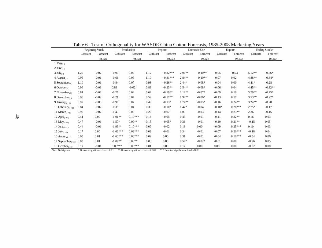
Table 6. Test of Orthogonality for WASDE China Cotton Forecasts, 1985-2008 Marketing Years

Constant Forecast

(M.Bal)

Constant Forecast

(M.Bal)

Constant Forecast

(M.Bal)

Constant Forecast

(M.Bal)

Constant Forecast

(M.Bal)

Constant Forecast

(M.Bal)

1 May(i )

2 June(i )

3 July(i ) 1.20 -0.02 -0.93 0.06 1.12 -0.32*** 2.96** -0.10** -0.05 -0.03 5.12** -0.36*

4 August(i ) 0.95 -0.01 -0.66 0.05 1.10 -0.31*** 2.84** -0.10** -0.07 0.02 4.88** -0.34*

5 September(i ) 1.10 -0.01 -0.84 0.07 0.98 -0.26** 2.44* -0.08* -0.04 0.00 4.41* -0.28

6 October(i ) 0.99 -0.03 0.83 -0.02 0.83 -0.23** 2.54** -0.08* -0.06 0.04 4.45** -0.32**

7 November(i ) 0.81 -0.02 -0.27 0.04 0.62 -0.19** 2.12** -0.07* -0.09 0.10 3.79** -0.25*

8 December(i ) 0.95 -0.02 -0.21 0.04 0.59 -0.17** 1.94** -0.06* -0.13 0.17 3.53** -0.22*

9 January(i +1) 0.99 -0.03 -0.98 0.07 0.49 -0.13* 1.74** -0.05* -0.16 0.24** 3.24** -0.20

10 February(i +1) 0.84 -0.02 -0.35 0.04 0.39 -0.10* 1.47* -0.04 -0.18* 0.28*** 2.75* -0.17

11 March(i +1) 0.90 -0.02 -1.43 0.08 0.20 -0.07 1.03 -0.03 -0.14 0.23** 2.26 -0.15

12 April(i +1) 0.41 0.00 -1.91** 0.10*** 0.18 -0.05 0.43 -0.01 -0.11 0.22** 0.16 0.03

13 May(i +1) 0.47 -0.01 -1.57* 0.09** 0.15 -0.05* 0.36 -0.01 -0.10 0.21** -0.15 0.05

14 June(i +1) 0.44 -0.01 -1.93** 0.10*** 0.09 -0.02 0.16 0.00 -0.09 0.25*** 0.10 0.03

15 July(i +1) 0.17 0.00 -1.63*** 0.08*** 0.09 -0.01 0.34 -0.01 -0.07 0.20*** -0.18 0.04

16 August(i +1) 0.05 0.01 -1.63*** 0.08*** 0.02 0.00 0.31 -0.01 -0.04 0.10*** -0.54 0.06

17 September(i +1) 0.05 0.01 -1.09** 0.06** 0.03 0.00 0.54* -0.02* -0.01 0.00 -0.26 0.05

18 October(i +1) 0.17 -0.01 0.00*** 0.00*** 0.01 0.00 0.17 0.00 0.00 0.00 -0.02 0.00

Note: N=24 years * Denotes significance level of 0.1 ** Denotes significance level of 0.05 *** Denotes significance level of 0.01

Beginning Stock Production Imports Domestic Use Exports Ending Stocks

46

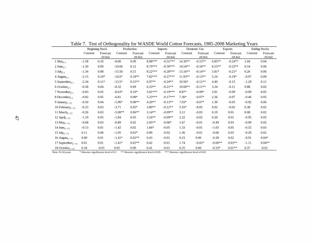
Table 7. Test of Orthogonality for WASDE World Cotton Forecasts, 1985-2008 Marketing Years

Constant Forecast (M.Bal)

Constant Forecast (M.Bal)

Constant Forecast (M.Bal)

Constant Forecast (M.Bal)

Constant Forecast (M.Bal)

Constant Forecast (M.Bal)

1 May(i ) -1.58 0.10 -8.00 0.09 8.98*** -0.31*** 14.30** -0.15** 6.85** -0.24** 1.04 0.04

2 June(i ) -1.50 0.09 -10.60 0.12 8.79*** -0.30*** 14.54** -0.16** 6.55** -0.23** 0.54 0.06

3 July(i ) -1.34 0.08 -13.50 0.15 8.22*** -0.28*** 13.16** -0.14** 5.81* -0.21* 0.26 0.06

4 August(i ) -2.15 0.10* -16.0* 0.18** 7.82*** -0.27*** 11.93** -0.13** 5.24 -0.19* -0.97 0.09

5 September(i ) -2.34 0.11* -13.5* 0.15** 6.97** -0.24** 10.56* -0.11** 4.40 -0.15 -1.29 0.11

6 October(i ) -0.58 0.04 -8.32 0.09 6.33** -0.21** 10.60** -0.11** 3.34 -0.11 0.88 0.02

7 November(i ) -0.83 0.05 -8.63* 0.10* 5.81*** -0.19*** 8.87* -0.09* 2.81 -0.09 -0.09 0.05

8 December(i ) -0.82 0.05 -6.81 0.08* 5.23*** -0.17*** 7.36* -0.07* 2.36 -0.07 -0.46 0.05

9 January(i +1) -0.50 0.04 -5.96* 0.08** 4.20** -0.13** 7.03* -0.07* 1.30 -0.03 -0.92 0.06

10 February(i +1) -0.23 0.03 -3.71 0.05* 3.80** -0.12** 5.55* -0.05 0.92 -0.02 0.38 0.02

11 March(i +1) -0.26 0.03 -5.00** 0.06** 3.14** -0.09** 3.12 -0.03 0.19 0.01 0.08 0.02

12 April(i +1) -1.19 0.05 -1.84 0.03 3.16** -0.09** 2.22 -0.02 0.20 0.01 -0.95 0.05

13 May(i +1) -0.68 0.03 -0.89 0.02 2.05** -0.06* 1.67 -0.01 -0.49 0.03 -0.09 0.02

14 June(i +1) -0.13 0.01 -1.42 0.02 1.66* -0.05 1.33 -0.01 -1.03 0.05 -0.55 0.03

15 July(i +1) 0.11 0.00 -1.05 0.02* 0.89 -0.02 1.36 -0.01 -0.68 0.03 -0.29 0.02

16 August(i +1) 0.00 0.01 -1.41* 0.02** 0.43 -0.01 0.23 0.00 -0.28 0.02 -0.91 0.04*

17 September(i +1) 0.01 0.01 -1.41* 0.02** 0.42 -0.01 1.74 -0.02* -0.69** 0.03** -1.11 0.04**

18 October(i +1) 0.34 -0.01 0.05 0.00 0.41 -0.01 0.25 0.00 -0.33* 0.01** 0.37 -0.01

Note: N=24 years * Denotes significance level of 0.1 ** Denotes significance level of 0.05 *** Denotes significance level of 0.01

Beginning Stock Production Imports Domestic Use Exports Ending Stocks

47

Table 8. Test of Weak Efficiency for WASDE U.S. Cotton Forecasts, 1985-2008 Marketing Years

Constant LagErrors

(M.Bal)

Constant LagErrors

(M.Bal)

Constant LagErrors

(M.Bal)

Constant LagErrors

(M.Bal)

Constant LagErrors

(¢/lb)

1 May(i ) 0.16 0.20 -0.06 0.41** 0.15 0.20 0.00 0.07 -2.40 -0.08

2 June(i ) 0.20 0.20 -0.04 0.43** 0.10 0.25 0.03 0.07 -2.49 -0.11

3 July(i ) 0.34 0.26 -0.02 0.51*** 0.23 0.23 0.05 0.11 -2.96* -0.03

4 August(i ) 0.06 0.21 -0.05 0.55*** 0.17 0.21 -0.09 0.28 -1.97 0.02

5 September(i ) 0.23 0.03 -0.05 0.52*** 0.18 0.22 0.05 0.17 -1.70 0.08

6 October(i ) 0.32 0.03 -0.04 0.43** 0.30 0.21 -0.01 0.22 -0.42 0.33

7 November(i ) 0.11 -0.02 -0.02 0.30 0.26 0.20 -0.16 0.17 0.13 0.32

8 December(i ) 0.05 -0.08 0.01 0.27 0.21 0.19 -0.21 0.10 -0.04 0.35

9 January(i +1) 0.01 -0.14 0.04 0.21 0.17 0.14 -0.23 0.09 -0.54 0.28

10 February(i +1) 0.01 -0.14 0.10 0.05 0.19 0.04 -0.31 -0.11 -0.76 0.14

11 March(i +1) 0.01 -0.13 0.09 -0.05 0.13 -0.03 -0.25 -0.26 -0.58* 0.05

12 April(i +1) 0.00 0.02 0.07 0.00 0.11 0.09 -0.21 -0.16 -0.53* 0.02

13 May(i +1) 0.00 -0.05 0.06 -0.01 0.08 0.15 -0.15 -0.01 -0.37 -0.16

14 June(i +1) 0.00 -0.05 0.07 -0.07 0.08 0.32 -0.15 0.10 -0.35 -0.18

15 July(i +1) 0.00 -0.05 0.09* -0.11 0.03 0.42** -0.10 0.11 -0.17 -0.26

16 August(i +1) 0.00 -0.05 0.04 -0.16 0.00 0.37* -0.05 -0.27 -0.25 -0.26

17 September(i +1) 0.00 -0.05 0.00 -0.31 0.00 0.27 0.01 -0.24 -0.18 -0.36

18 October(i +1) 0.00 -0.05 0.00 0.02 0.00 -0.05 0.00 0.00 -0.06 -0.06

Note: N=24 years * Denotes significance level of 0.1 ** Denotes significance level of 0.05 *** Denotes significance level of 0.01

Production Domestic Use Exports Ending Stock Price

48

Table 9. Test of Weak Efficiency for WASDE China Cotton Forecasts, 1985-2008 Marketing Years

Constant LagErrors

(M.Bal)

Constant LagErrors

(M.Bal)

Constant LagErrors

(M.Bal)

Constant LagErrors

(M.Bal)

Constant LagErrors

(M.Bal)

Constant LagErrors

(M.Bal)

1 May(i )

2 June(i )

3 July(i ) 0.64 0.30 0.41 0.24 -0.14 0.23 -0.32 0.86*** -0.12 0.12 0.85 0.29

4 August(i ) 0.62 0.31 0.49 0.18 -0.08 0.17 -0.28 0.84*** -0.10 0.15 0.91 0.29

5 September(i ) 0.70 0.25 0.70 0.17 -0.01 0.07 -0.20 0.78** -0.09 -0.08 1.08 0.30

6 October(i ) 0.54 0.14 0.56 0.11 -0.03 0.12 -0.17 0.74** -0.09 -0.02 0.86 0.24

7 November(i ) 0.54 0.19 0.74* 0.22 -0.10 0.09 -0.05 0.60** -0.07 0.02 0.99 0.29

8 December(i ) 0.58 0.16 0.80** 0.17 -0.05 0.09 0.14 0.40 -0.06 0.09 1.02* 0.28

9 January(i +1) 0.58 0.18 0.74** 0.21 0.03 -0.09 0.20 0.29 -0.04 0.23 0.99* 0.35*

10 February(i +1) 0.63 -0.05 0.72** 0.11 0.01 -0.21 0.47 -0.12 -0.03 0.34** 0.84* 0.28

11 March(i +1) 0.64 -0.03 0.48** 0.23 -0.06 -0.22 0.46 -0.23 -0.02 0.39** 0.65 0.33*

12 April(i +1) 0.37 0.15 0.34 0.29 -0.01 -0.15 0.39 -0.52** -0.01 0.33* 0.48 0.32

13 May(i +1) 0.29 0.03 0.37 0.16 -0.04 0.00 0.30 -0.54*** -0.01 0.34** 0.45 0.21

14 June(i +1) 0.37 -0.01 0.23 0.23 0.03 0.08 0.21 -0.55*** 0.02 0.40** 0.33 0.52***

15 July(i +1) 0.18 -0.07 0.15 0.39* 0.04 0.22 0.13 -0.57*** 0.02 0.38** 0.21 0.51**

16 August(i +1) 0.15 -0.04 0.15 0.39* 0.01 0.10 0.18 -0.57*** 0.01 0.37** 0.18 0.49**

17 September(i +1) 0.15 -0.04 0.18 -0.06 0.03 -0.14 -0.05 -0.20 -0.01 0.04 0.24 0.29

18 October(i +1) 0.03 -0.20 0.00*** 0.00*** 0.01 -0.07 0.07 -0.14 0.00 -0.08 -0.05 -0.27

Note: N=24 years * Denotes significance level of 0.1 ** Denotes significance level of 0.05 *** Denotes significance level of 0.01

Beginning stock Production Import Domestic Use Export Ending Stock

49

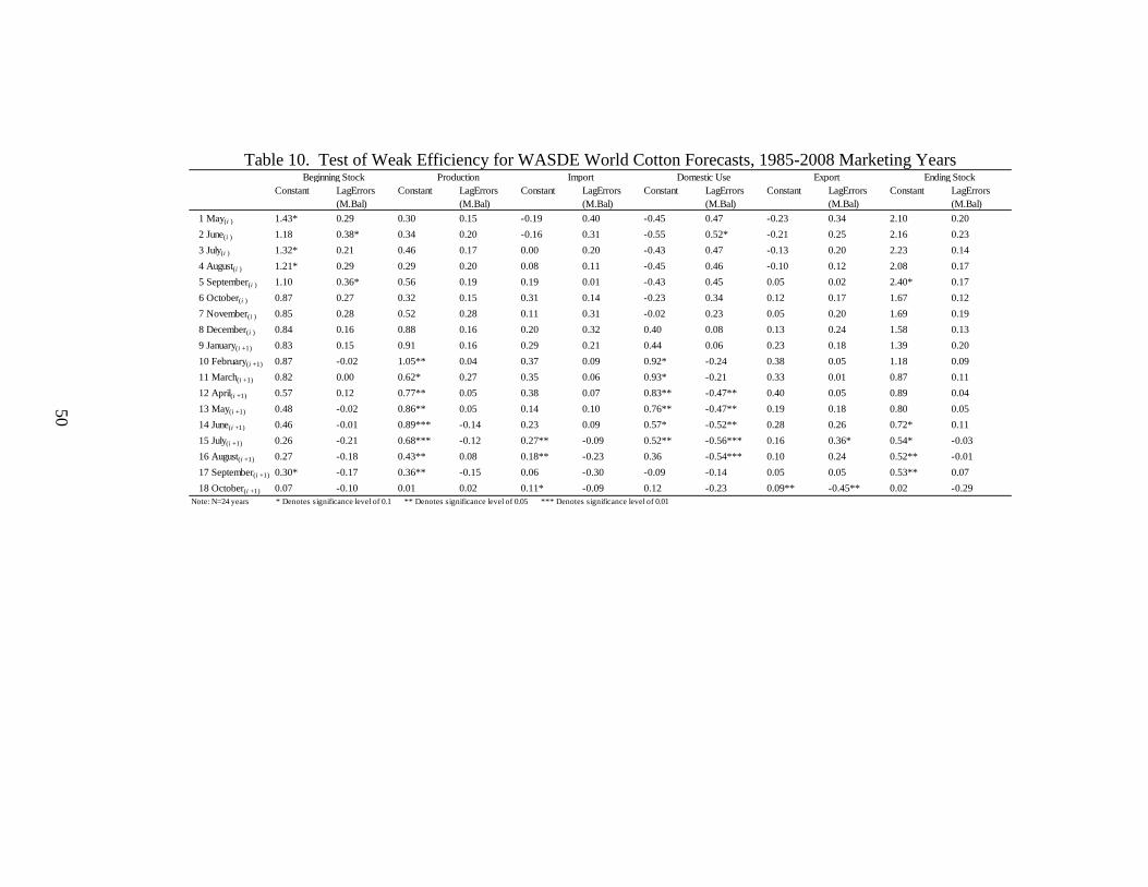
Table 10. Test of Weak Efficiency for WASDE World Cotton Forecasts, 1985-2008 Marketing Years

Constant LagErrors

(M.Bal)

Constant LagErrors

(M.Bal)

Constant LagErrors

(M.Bal)

Constant LagErrors

(M.Bal)

Constant LagErrors

(M.Bal)

Constant LagErrors

(M.Bal)

1 May(i ) 1.43* 0.29 0.30 0.15 -0.19 0.40 -0.45 0.47 -0.23 0.34 2.10 0.20

2 June(i ) 1.18 0.38* 0.34 0.20 -0.16 0.31 -0.55 0.52* -0.21 0.25 2.16 0.23

3 July(i ) 1.32* 0.21 0.46 0.17 0.00 0.20 -0.43 0.47 -0.13 0.20 2.23 0.14

4 August(i ) 1.21* 0.29 0.29 0.20 0.08 0.11 -0.45 0.46 -0.10 0.12 2.08 0.17

5 September(i ) 1.10 0.36* 0.56 0.19 0.19 0.01 -0.43 0.45 0.05 0.02 2.40* 0.17

6 October(i ) 0.87 0.27 0.32 0.15 0.31 0.14 -0.23 0.34 0.12 0.17 1.67 0.12

7 November(i ) 0.85 0.28 0.52 0.28 0.11 0.31 -0.02 0.23 0.05 0.20 1.69 0.19

8 December(i ) 0.84 0.16 0.88 0.16 0.20 0.32 0.40 0.08 0.13 0.24 1.58 0.13

9 January(i +1) 0.83 0.15 0.91 0.16 0.29 0.21 0.44 0.06 0.23 0.18 1.39 0.20

10 February(i +1) 0.87 -0.02 1.05** 0.04 0.37 0.09 0.92* -0.24 0.38 0.05 1.18 0.09

11 March(i +1) 0.82 0.00 0.62* 0.27 0.35 0.06 0.93* -0.21 0.33 0.01 0.87 0.11

12 April(i +1) 0.57 0.12 0.77** 0.05 0.38 0.07 0.83** -0.47** 0.40 0.05 0.89 0.04

13 May(i +1) 0.48 -0.02 0.86** 0.05 0.14 0.10 0.76** -0.47** 0.19 0.18 0.80 0.05

14 June(i +1) 0.46 -0.01 0.89*** -0.14 0.23 0.09 0.57* -0.52** 0.28 0.26 0.72* 0.11

15 July(i +1) 0.26 -0.21 0.68*** -0.12 0.27** -0.09 0.52** -0.56*** 0.16 0.36* 0.54* -0.03

16 August(i +1) 0.27 -0.18 0.43** 0.08 0.18** -0.23 0.36 -0.54*** 0.10 0.24 0.52** -0.01

17 September(i +1) 0.30* -0.17 0.36** -0.15 0.06 -0.30 -0.09 -0.14 0.05 0.05 0.53** 0.07

18 October(i +1) 0.07 -0.10 0.01 0.02 0.11* -0.09 0.12 -0.23 0.09** -0.45** 0.02 -0.29

Note: N=24 years * Denotes significance level of 0.1 ** Denotes significance level of 0.05 *** Denotes significance level of 0.01

Beginning Stock Production Import Domestic Use Export Ending Stock

50

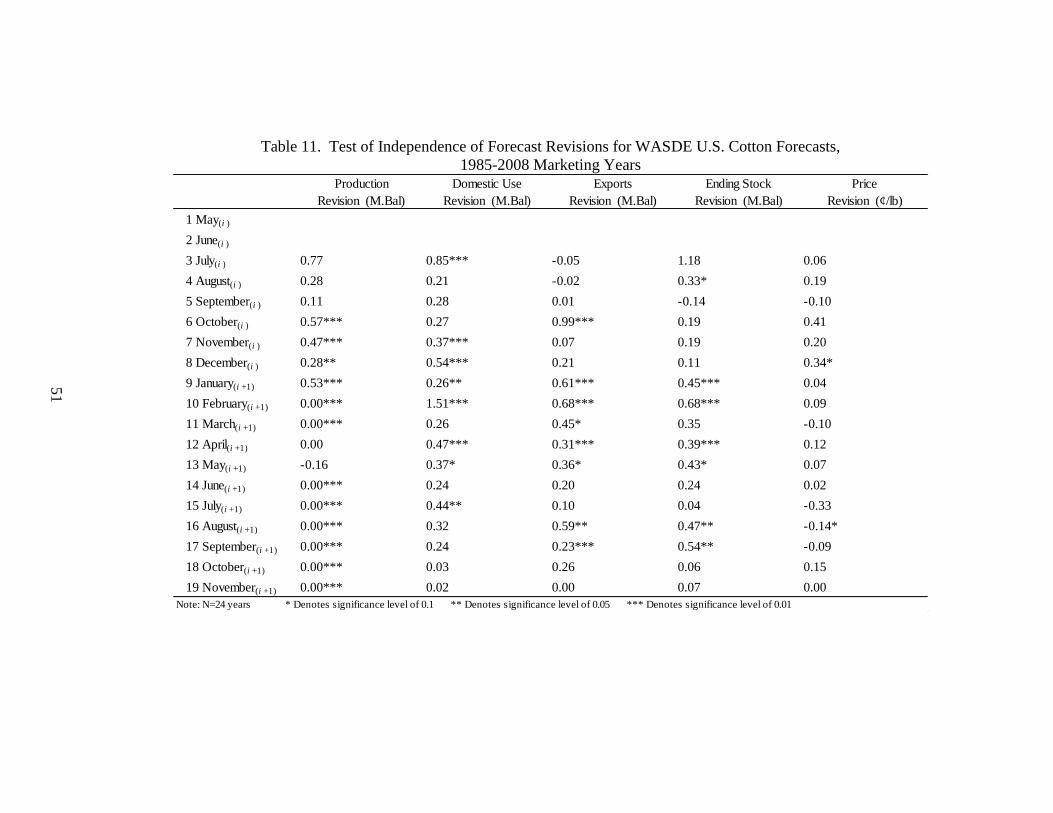
Table 11. Test of Independence of Forecast Revisions for WASDE U.S. Cotton Forecasts,

1985-2008 Marketing Years Production Domestic Use Exports Ending Stock Price

Revision (M.Bal) Revision (M.Bal) Revision (M.Bal) Revision (M.Bal) Revision (¢/lb)

1 May(i )

2 June(i )

3 July(i ) 0.77 0.85*** -0.05 1.18 0.06

4 August(i ) 0.28 0.21 -0.02 0.33* 0.19

5 September(i ) 0.11 0.28 0.01 -0.14 -0.10

6 October(i ) 0.57*** 0.27 0.99*** 0.19 0.41

7 November(i ) 0.47*** 0.37*** 0.07 0.19 0.20

8 December(i ) 0.28** 0.54*** 0.21 0.11 0.34*

9 January(i +1) 0.53*** 0.26** 0.61*** 0.45*** 0.04

10 February(i +1) 0.00*** 1.51*** 0.68*** 0.68*** 0.09

11 March(i +1) 0.00*** 0.26 0.45* 0.35 -0.10

12 April(i +1) 0.00 0.47*** 0.31*** 0.39*** 0.12

13 May(i +1) -0.16 0.37* 0.36* 0.43* 0.07

14 June(i +1) 0.00*** 0.24 0.20 0.24 0.02

15 July(i +1) 0.00*** 0.44** 0.10 0.04 -0.33

16 August(i +1) 0.00*** 0.32 0.59** 0.47** -0.14*

17 September(i +1) 0.00*** 0.24 0.23*** 0.54** -0.09

18 October(i +1) 0.00*** 0.03 0.26 0.06 0.15

19 November(i +1) 0.00*** 0.02 0.00 0.07 0.00

Note: N=24 years * Denotes significance level of 0.1 ** Denotes significance level of 0.05 *** Denotes significance level of 0.01

51

Table 12. Test of Independence of Forecast Revisions for WASDE China Cotton Forecasts,

1985-2008 Marketing Years Beginning Stock Production Imports Domestic Use Exports Ending Stocks

Revision (M.Bal) Revision (M.Bal) Revision (M.Bal) Revision (M.Bal) Revision (M.Bal) Revision (M.Bal)

1 May(i )

2 June(i )

3 July(i )

4 August(i )

5 September(i ) -0.09 0.76** 1.61*** 0.27 0.39 0.16

6 October(i ) -0.12 0.18 0.73*** 0.51** 0.00 -0.26

7 November(i ) 0.00 -0.10 0.93*** 0.23 0.00 -0.19

8 December(i ) 0.03 0.03 0.13 0.53*** 0.13 0.02

9 January(i +1) 0.00 0.77 0.98*** 0.48*** 0.54*** 0.62*

10 February(i +1) 0.00 -0.06 0.55*** 0.95** 0.70** -0.30

11 March(i +1) 0.00 0.03 0.44 0.22* 0.43*** 0.05

12 April(i +1) 0.00 0.00 0.20** 0.28 0.19 0.12

13 May(i +1) 0.06 0.00 0.44** 0.09 0.11 -0.03

14 June(i +1) 0.00 0.00 0.46 0.01 0.87 -0.41**

15 July(i +1) 0.01 0.00 0.33*** 0.04 0.16* -0.30

16 August(i +1) 0.00 0.00*** -0.18 -0.08 1.16*** 0.02

17 September(i +1) 0.00 0.00*** 0.02 -1.34* 0.75*** -0.12

18 October(i +1) -230.00 0.00 0.02 0.18 0.02 -0.12

19 November(i +1) 0.00 0.00*** 0.00 0.01 0.00 0.00

Note: N=24 years * Denotes significance level of 0.1 ** Denotes significance level of 0.05 *** Denotes significance level of 0.01

52

Table 13. Test of Independence of Forecast Revisions for WASDE World Cotton Forecasts,

1985-2008 Marketing Years Beginning Stock Production Imports Domestic Use Exports Ending Stocks

Revision (M.Bal) Revision (M.Bal) Revision (M.Bal) Revision (M.Bal) Revision (M.Bal) Revision (M.Bal)

1 May(i )

2 June(i )

3 July(i ) 0.36 0.44 0.07 0.07 0.14 0.43

4 August(i ) 0.16 0.34** -0.05 0.36** -0.01 0.25*

5 September(i ) -0.01 0.23 0.45** 0.53*** 0.48** 0.08

6 October(i ) -0.72 0.23 0.92** 1.17*** 0.79** -0.26

7 November(i ) 0.00 -0.16 0.35** 0.49** 0.39** -0.11

8 December(i ) -0.13 0.28** 0.29 0.71*** 0.32 0.05

9 January(i +1) 0.02 0.48** 0.61*** 0.44*** 0.56*** 0.53**

10 February(i +1) 0.05 0.15 0.79*** 1.34*** 0.76*** -0.04

11 March(i +1) 0.07 0.31 0.34 0.31** 0.36* 0.49**

12 April(i +1) 0.27 0.04 0.22** 0.26 0.16 0.12

13 May(i +1) 0.17 0.02 -0.26 0.12 0.31 0.07

14 June(i +1) 0.17 -0.44 -0.09 -0.12 -0.18*** 0.00

15 July(i +1) 0.08 0.20 0.47 0.18 -0.01 0.27

16 August(i +1) 0.01 0.38*** 0.10 0.17 0.30 0.16

17 September(i +1) -0.27** -0.12 0.14 0.22 0.23 -0.02

18 October(i +1) 0.04 0.01 0.03 0.10 0.01 -0.81*

19 November(i +1) 0.15 -0.07* -0.30 -0.04 0.19 -0.05

Note: N=24 years * Denotes significance level of 0.1 ** Denotes significance level of 0.05 *** Denotes significance level of 0.01

53

Table 14. USDA WASDE Forecast Evaluation Summary for 1985-2008 Marketing Years

Most Significant Categories found within the Forecasting Evaluation Framework (By Region) Region Test Beginning Stocks

(M.Bal)

Production

(M.Bal)

Imports

(M.Bal)

Domestic Use

(M.Bal)

Exports

(M.Bal)

Ending Stocks

(M.Bal)

Price

(¢/lb)

U.S. Test of Bias X

Test of Orthogonality X

Test of Weak Efficiency X

Test of Revisions X

China Test of Bias X

Test of Orthogonality X

Test of Weak Efficiency X

Test of Revisions X

World Test of Bias X

Test of Orthogonality X

Test of Weak Efficiency X

Test of Revisions X

54

Table 15. Evaluation for the Adjustment of Bias in USDA WASDE U.S. Domestic Use Forecasts,

1999-2008 Marketing Years

Month

Original M.BalAdjusted

M.Bal

Improvement

M.BalOriginal M.Bal

Adjusted

M.Bal

Improvement

M.Bal

1 May(i ) 0.73 0.60 0.12 0.80 0.81 -0.01

2 June(i ) 0.68 0.56 0.12 0.74 0.76 -0.02

3 July(i ) 0.61 0.52 0.09 0.68 0.72 -0.04

4 August(i ) 0.56 0.48 0.08 0.66 0.66 0.00

5 September(i ) 0.51 0.46 0.04 0.62 0.61 0.02

6 October(i ) 0.49 0.44 0.04 0.61 0.57 0.03

7 November(i ) 0.44 0.44 0.00 0.55 0.54 0.00

8 December(i ) 0.36 0.41 -0.05 0.48 0.48 -0.01

9 January(i +1) 0.32 0.39 -0.07 0.44 0.46 -0.02

10 February(i +1) 0.31 0.35 -0.05 0.39 0.43 -0.04

11 March(i +1) 0.27 0.32 -0.05 0.34 0.37 -0.04

12 April(i +1) 0.24 0.29 -0.05 0.30 0.32 -0.02

13 May(i +1) 0.20 0.26 -0.06 0.27 0.30 -0.03

14 June(i +1) 0.17 0.21 -0.04 0.25 0.27 -0.02

15 July(i +1)

16 August(i +1)

17 September(i +1)

18 October(i +1)

0.12 -0.19

Mean Absolute Error Root Mean Square Error

MAE Overall Improvement RMSE Overall Improvement

55

Table 16. Evaluation for the Adjustment of Bias in USDA WASDE China Ending Stock Forecasts,

1999-2008 Marketing Years

Month

Original M.BalAdjusted

M.Bal

Improvement

M.BalOriginal M.Bal

Adjusted

M.Bal

Improvement

M.Bal

1 May(i )

2 June(i )

3 July(i ) 3.27 2.51 0.75 3.98 3.14 0.84

4 August(i ) 3.19 2.22 0.98 3.92 2.74 1.18

5 September(i ) 3.11 2.52 0.59 3.93 2.90 1.03

6 October(i ) 2.29 2.31 -0.01 2.84 2.85 -0.02

7 November(i ) 2.16 2.20 -0.04 2.63 2.66 -0.04

8 December(i ) 2.12 1.95 0.17 2.58 2.40 0.19

9 January(i +1) 2.38 1.70 0.68 2.90 2.08 0.83

10 February(i +1) 2.00 1.33 0.66 2.22 1.73 0.49

11 March(i +1) 2.11 1.39 0.71 2.44 1.87 0.57

12 April(i +1) 2.07 1.69 0.38 2.49 1.93 0.56

13 May(i +1) 1.56 1.07 0.50 1.75 1.32 0.43

14 June(i +1) 1.76 1.32 0.43 2.12 1.47 0.65

15 July(i +1) 1.14 0.98 0.16 1.57 1.28 0.30

16 August(i +1) 1.12 0.90 0.22 1.61 1.32 0.29

17 September(i +1) 0.99 1.00 -0.01 1.58 1.41 0.17

18 October(i +1)

6.18 7.47MAE Overall Improvement RMSE Overall Improvement

Mean Absolute Error Root Mean Square Error

56

Table 17. Evaluation for the Adjustment of Bias in USDA WASDE World Import Forecasts,

1999-2008 Marketing Years

Month

Original M.Bal

Adjusted

M.Bal

Improvement

M.Bal Original M.Bal

Adjusted

M.Bal

Improvement

M.Bal

1 May(i ) 3.72 3.76 -0.04 4.82 4.85 -0.02

2 June(i ) 3.60 3.63 -0.03 4.75 4.75 -0.01

3 July(i ) 3.57 3.75 -0.18 4.60 4.73 -0.14

4 August(i ) 3.35 3.42 -0.07 4.35 4.46 -0.11

5 September(i ) 3.02 3.07 -0.05 3.99 4.11 -0.12

6 October(i ) 2.62 2.45 0.17 3.25 3.32 -0.07

7 November(i ) 2.20 2.00 0.20 2.75 2.72 0.03

8 December(i ) 1.88 1.66 0.23 2.30 2.30 0.00

9 January(i +1) 1.44 1.36 0.08 1.84 1.88 -0.04

10 February(i +1) 1.26 1.33 -0.07 1.57 1.66 -0.09

11 March(i +1) 0.82 0.90 -0.08 1.00 1.09 -0.09

12 April(i +1) 0.76 0.83 -0.07 0.84 0.96 -0.12

13 May(i +1) 0.57 0.73 -0.17 0.72 0.91 -0.18

14 June(i +1) 0.54 0.65 -0.11 0.70 0.81 -0.11

15 July(i +1)

16 August(i +1) 0.21 0.20 0.01 0.31 0.30 0.01

17 September(i +1) 0.25 0.26 -0.01 0.32 0.35 -0.03

18 October(i +1)

-0.19 -1.07MAE Overall Improvement RMSE Overall Improvement

Mean Absolute Error Root Mean Square Error

57

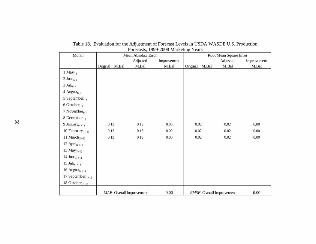
Table 18. Evaluation for the Adjustment of Forecast Levels in USDA WASDE U.S. Production

Forecasts, 1999-2008 Marketing Years

Month

Original M.Bal

Adjusted

M.Bal

Improvement

M.Bal Original M.Bal

Adjusted

M.Bal

Improvement

M.Bal

1 May(i )

2 June(i )

3 July(i )

4 August(i )

5 September(i )

6 October(i )

7 November(i )

8 December(i )

9 January(i +1) 0.13 0.13 0.00 0.02 0.02 0.00

10 February(i +1) 0.13 0.13 0.00 0.02 0.02 0.00

11 March(i +1) 0.13 0.13 0.00 0.02 0.02 0.00

12 April(i +1)

13 May(i +1)

14 June(i +1)

15 July(i +1)

16 August(i +1)

17 September(i +1)

18 October(i +1)

0.00 0.00MAE Overall Improvement RMSE Overall Improvement

Mean Absolute Error Root Mean Square Error

58

Table 19. Evaluation for the Adjustment of Forecast Levels in USDA WASDE China Import

Forecasts, 1999-2008 Marketing Years

Month

Original M.Bal

Adjusted

M.Bal

Improvement

M.Bal Original M.Bal

Adjusted

M.Bal

Improvement

M.Bal

1 May(i )

2 June(i )

3 July(i ) 3.56 3.64 -0.08 4.74 5.85 -1.11

4 August(i ) 3.37 3.60 -0.22 4.57 5.81 -1.24

5 September(i ) 2.95 3.26 -0.32 4.10 5.35 -1.25

6 October(i ) 2.61 2.84 -0.23 3.57 4.45 -0.89

7 November(i ) 2.18 2.32 -0.14 2.94 3.52 -0.58

8 December(i ) 1.95 2.05 -0.11 2.68 3.22 -0.55

9 January(i +1) 1.66 1.89 -0.24 2.31 3.03 -0.72

10 February(i +1) 1.53 1.73 -0.20 2.11 2.75 -0.64

11 March(i +1)

12 April(i +1)

13 May(i +1) 0.62 0.84 -0.22 0.96 1.20 -0.24

14 June(i +1)

15 July(i +1)

16 August(i +1)

17 September(i +1)

18 October(i +1)

-1.74 -7.22MAE Overall Improvement RMSE Overall Improvement

Mean Absolute Error Root Mean Square Error

59

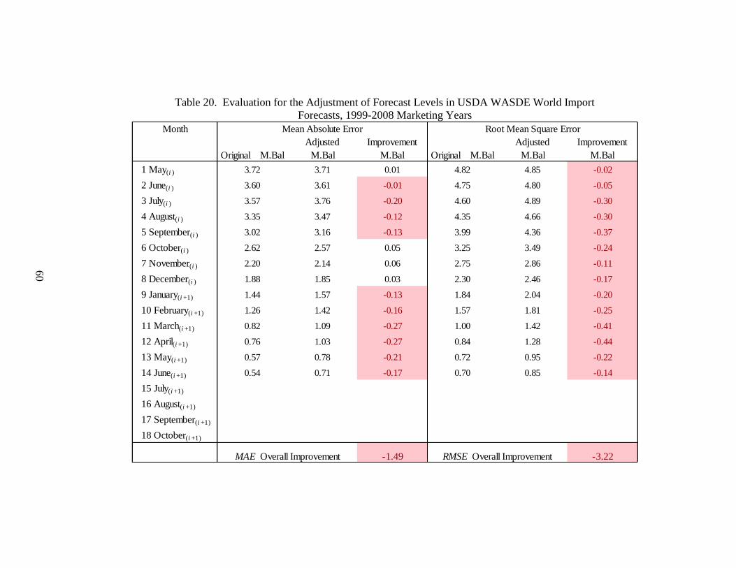
Table 20. Evaluation for the Adjustment of Forecast Levels in USDA WASDE World Import

Forecasts, 1999-2008 Marketing Years

Month

Original M.Bal

Adjusted

M.Bal

Improvement

M.Bal Original M.Bal

Adjusted

M.Bal

Improvement

M.Bal

1 May(i ) 3.72 3.71 0.01 4.82 4.85 -0.02

2 June(i ) 3.60 3.61 -0.01 4.75 4.80 -0.05

3 July(i ) 3.57 3.76 -0.20 4.60 4.89 -0.30

4 August(i ) 3.35 3.47 -0.12 4.35 4.66 -0.30

5 September(i ) 3.02 3.16 -0.13 3.99 4.36 -0.37

6 October(i ) 2.62 2.57 0.05 3.25 3.49 -0.24

7 November(i ) 2.20 2.14 0.06 2.75 2.86 -0.11

8 December(i ) 1.88 1.85 0.03 2.30 2.46 -0.17

9 January(i +1) 1.44 1.57 -0.13 1.84 2.04 -0.20

10 February(i +1) 1.26 1.42 -0.16 1.57 1.81 -0.25

11 March(i +1) 0.82 1.09 -0.27 1.00 1.42 -0.41

12 April(i +1) 0.76 1.03 -0.27 0.84 1.28 -0.44

13 May(i +1) 0.57 0.78 -0.21 0.72 0.95 -0.22

14 June(i +1) 0.54 0.71 -0.17 0.70 0.85 -0.14

15 July(i +1)

16 August(i +1)

17 September(i +1)

18 October(i +1)

-1.49 -3.22MAE Overall Improvement RMSE Overall Improvement

Mean Absolute Error Root Mean Square Error

60

Table 21. Evaluation for the Adjustment of Lagged Errors in USDA WASDE U.S. Domestic Use

Forecasts, 1999-2008 Marketing Years

Month

Original M.Bal

Adjusted

M.Bal

Improvement

M.Bal Original M.Bal

Adjusted

M.Bal

Improvement

M.Bal

1 May(i ) 0.73 0.73 -0.01 0.80 0.81 -0.01

2 June(i ) 0.68 0.66 0.01 0.74 0.76 -0.02

3 July(i ) 0.61 0.54 0.07 0.68 0.69 -0.01

4 August(i ) 0.56 0.51 0.05 0.66 0.63 0.03

5 September(i ) 0.51 0.50 0.01 0.62 0.61 0.02

6 October(i ) 0.49 0.46 0.02 0.61 0.62 -0.02

7 November(i )

8 December(i )

9 January(i +1)

10 February(i +1)

11 March(i +1)

12 April(i +1)

13 May(i +1)

14 June(i +1)

15 July(i +1)

16 August(i +1)

17 September(i +1)

18 October(i +1)

0.15 0.00MAE Overall Improvement RMSE Overall Improvement

Mean Absolute Error Root Mean Square Error

61

Table 22. Evaluation for the Adjustment of Lagged Errors in USDA WASDE China Domestic Use

Forecasts, 1999-2008 Marketing Years

Month

Original M.Bal

Adjusted

M.Bal

Improvement

M.Bal Original M.Bal

Adjusted

M.Bal

Improvement

M.Bal

1 May(i )

2 June(i )

3 July(i ) 2.99 2.43 0.56 3.72 3.21 0.51

4 August(i ) 2.79 2.26 0.53 3.48 3.05 0.43

5 September(i ) 2.65 2.13 0.52 3.32 2.94 0.38

6 October(i ) 2.80 2.29 0.51 3.35 3.09 0.26

7 November(i ) 2.31 2.06 0.25 2.72 2.61 0.11

8 December(i )

9 January(i +1)

10 February(i +1)

11 March(i +1)

12 April(i +1) 1.31 1.33 -0.02 1.62 1.53 0.09

13 May(i +1) 1.42 1.66 -0.25 2.09 2.16 -0.08

14 June(i +1) 1.26 1.54 -0.29 2.03 2.23 -0.20

15 July(i +1) 1.00 0.96 0.04 1.63 1.47 0.16

16 August(i +1) 0.95 1.01 -0.06 1.69 1.62 0.08

17 September(i +1)

18 October(i +1)

1.79 1.75RMSE Overall ImprovementMAE Overall Improvement

Mean Absolute Error Root Mean Square Error

62

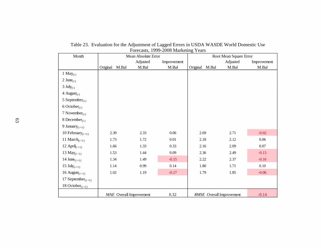
Table 23. Evaluation for the Adjustment of Lagged Errors in USDA WASDE World Domestic Use

Forecasts, 1999-2008 Marketing Years

Month

Original M.Bal

Adjusted

M.Bal

Improvement

M.Bal Original M.Bal

Adjusted

M.Bal

Improvement

M.Bal

1 May(i )

2 June(i )

3 July(i )

4 August(i )

5 September(i )

6 October(i )

7 November(i )

8 December(i )

9 January(i +1)

10 February(i +1) 2.39 2.33 0.06 2.69 2.71 -0.02

11 March(i +1) 1.73 1.72 0.01 2.18 2.12 0.06

12 April(i +1) 1.66 1.33 0.33 2.16 2.09 0.07

13 May(i +1) 1.53 1.44 0.09 2.36 2.49 -0.13

14 June(i +1) 1.34 1.49 -0.15 2.22 2.37 -0.16

15 July(i +1) 1.14 0.99 0.14 1.80 1.71 0.10

16 August(i +1) 1.02 1.19 -0.17 1.79 1.85 -0.06

17 September(i +1)

18 October(i +1)

0.32 -0.14MAE Overall Improvement RMSE Overall Improvement

Mean Absolute Error Root Mean Square Error

63

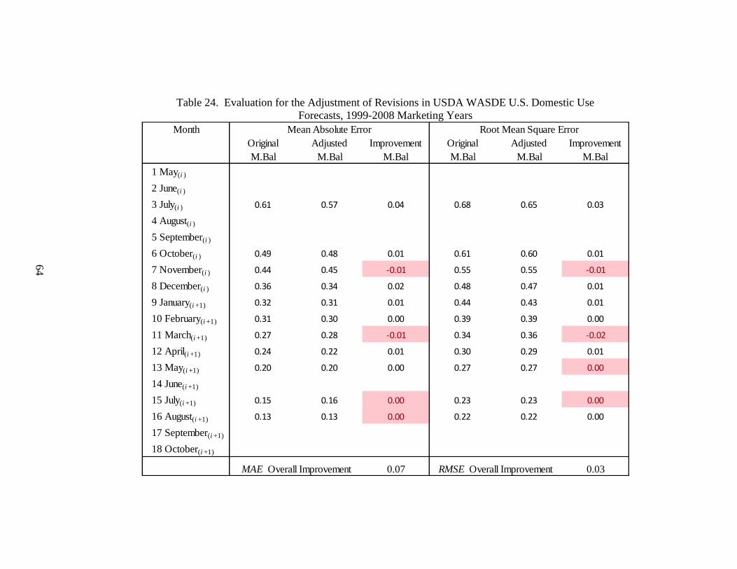
Table 24. Evaluation for the Adjustment of Revisions in USDA WASDE U.S. Domestic Use

Forecasts, 1999-2008 Marketing Years

Month

Original

M.Bal

Adjusted

M.Bal

Improvement

M.Bal

Original

M.Bal

Adjusted

M.Bal

Improvement

M.Bal

1 May(i )

2 June(i )

3 July(i ) 0.61 0.57 0.04 0.68 0.65 0.03

4 August(i )

5 September(i )

6 October(i ) 0.49 0.48 0.01 0.61 0.60 0.01

7 November(i ) 0.44 0.45 -0.01 0.55 0.55 -0.01

8 December(i ) 0.36 0.34 0.02 0.48 0.47 0.01

9 January(i +1) 0.32 0.31 0.01 0.44 0.43 0.01

10 February(i +1) 0.31 0.30 0.00 0.39 0.39 0.00

11 March(i +1) 0.27 0.28 -0.01 0.34 0.36 -0.02

12 April(i +1) 0.24 0.22 0.01 0.30 0.29 0.01

13 May(i +1) 0.20 0.20 0.00 0.27 0.27 0.00

14 June(i +1)

15 July(i +1) 0.15 0.16 0.00 0.23 0.23 0.00

16 August(i +1) 0.13 0.13 0.00 0.22 0.22 0.00

17 September(i +1)

18 October(i +1)

0.07 0.03MAE Overall Improvement RMSE Overall Improvement

Mean Absolute Error Root Mean Square Error

64

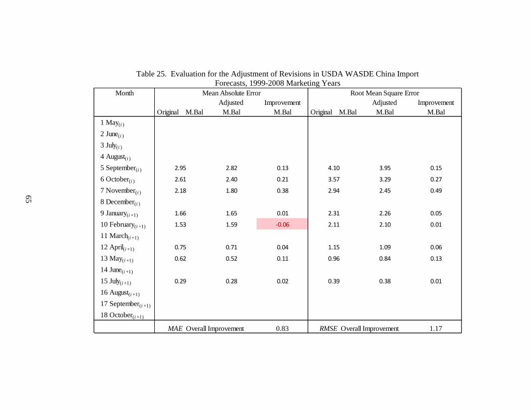
Table 25. Evaluation for the Adjustment of Revisions in USDA WASDE China Import

Forecasts, 1999-2008 Marketing Years

Month

Original M.Bal

Adjusted

M.Bal

Improvement

M.Bal Original M.Bal

Adjusted

M.Bal

Improvement

M.Bal

1 May(i )

2 June(i )

3 July(i )

4 August(i )

5 September(i ) 2.95 2.82 0.13 4.10 3.95 0.15

6 October(i ) 2.61 2.40 0.21 3.57 3.29 0.27

7 November(i ) 2.18 1.80 0.38 2.94 2.45 0.49

8 December(i )

9 January(i +1) 1.66 1.65 0.01 2.31 2.26 0.05

10 February(i +1) 1.53 1.59 -0.06 2.11 2.10 0.01

11 March(i +1)

12 April(i +1) 0.75 0.71 0.04 1.15 1.09 0.06

13 May(i +1) 0.62 0.52 0.11 0.96 0.84 0.13

14 June(i +1)

15 July(i +1) 0.29 0.28 0.02 0.39 0.38 0.01

16 August(i +1)

17 September(i +1)

18 October(i +1)

0.83 1.17MAE Overall Improvement RMSE Overall Improvement

Mean Absolute Error Root Mean Square Error

65

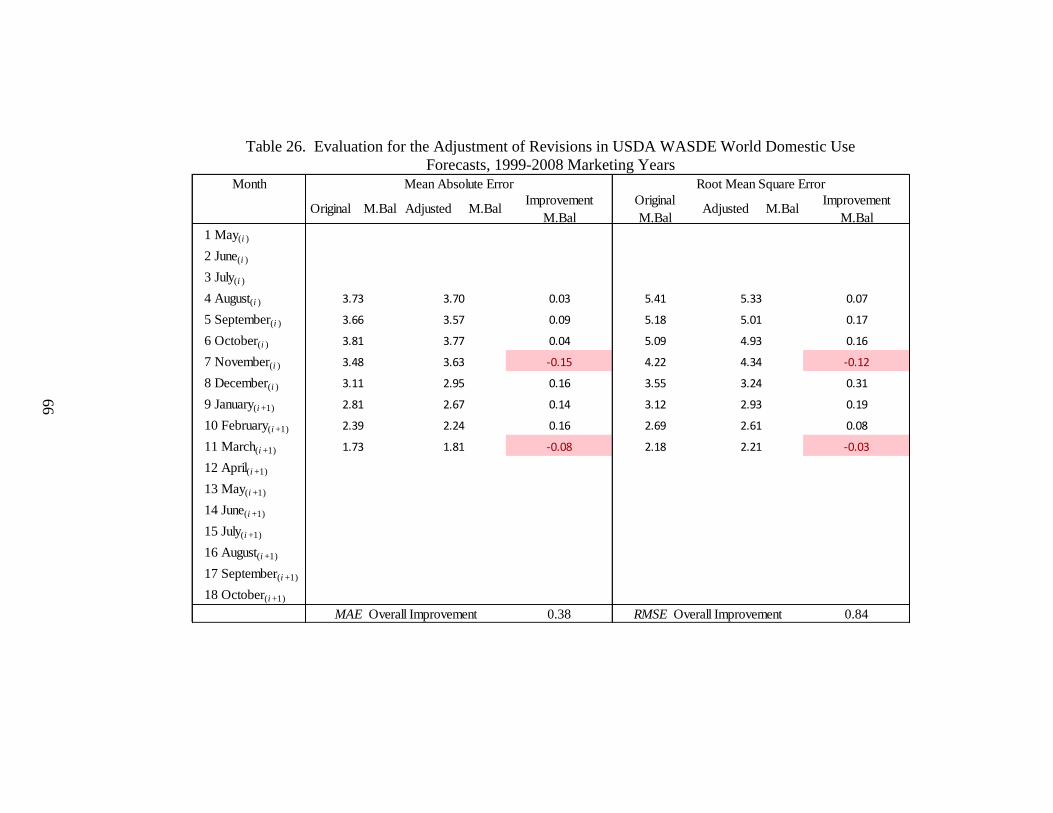
Table 26. Evaluation for the Adjustment of Revisions in USDA WASDE World Domestic Use

Forecasts, 1999-2008 Marketing Years

Month

Original M.Bal Adjusted M.BalImprovement

M.Bal

Original

M.BalAdjusted M.Bal

Improvement

M.Bal

1 May(i )

2 June(i )

3 July(i )

4 August(i ) 3.73 3.70 0.03 5.41 5.33 0.07

5 September(i ) 3.66 3.57 0.09 5.18 5.01 0.17

6 October(i ) 3.81 3.77 0.04 5.09 4.93 0.16

7 November(i ) 3.48 3.63 -0.15 4.22 4.34 -0.12

8 December(i ) 3.11 2.95 0.16 3.55 3.24 0.31

9 January(i +1) 2.81 2.67 0.14 3.12 2.93 0.19

10 February(i +1) 2.39 2.24 0.16 2.69 2.61 0.08

11 March(i +1) 1.73 1.81 -0.08 2.18 2.21 -0.03

12 April(i +1)

13 May(i +1)

14 June(i +1)

15 July(i +1)

16 August(i +1)

17 September(i +1)

18 October(i +1)

0.38 0.84MAE Overall Improvement RMSE Overall Improvement

Mean Absolute Error Root Mean Square Error

66

67

Figure 1. WASDE Forecasting Cycle for Cotton 2006/07 Marketing Year

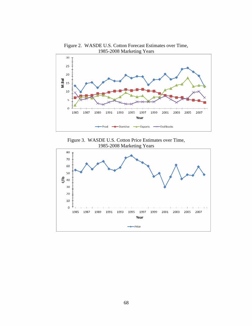
68

Figure 2. WASDE U.S. Cotton Forecast Estimates over Time,

1985-2008 Marketing Years

Figure 3. WASDE U.S. Cotton Price Estimates over Time,

1985-2008 Marketing Years

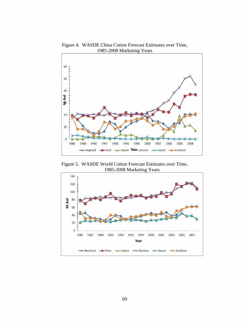
69

Figure 4. WASDE China Cotton Forecast Estimates over Time,

1985-2008 Marketing Years

Figure 5. WASDE World Cotton Forecast Estimates over Time,

1985-2008 Marketing Years

70

APPENDICES

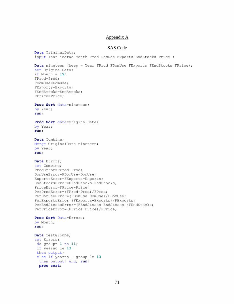
71

Appendix A

SAS Code Data OriginalData;

input Year YearNo Month Prod DomUse Exports EndStocks Price ;

Data nineteen (keep = Year FProd FDomUse FExports FEndStocks FPrice);

set OriginalData;

if Month = 19;

FProd=Prod;

FDomUse=DomUse;

FExports=Exports;

FEndStocks=EndStocks;

FPrice=Price;

Proc Sort data=nineteen;

by Year;

run;

Proc Sort data=OriginalData;

by Year;

run;

Data Combine;

Merge OriginalData nineteen;

by Year;

run;

Data Errors;

set Combine;

ProdError=FProd-Prod;

DomUseError=FDomUse-DomUse;

ExportsError=FExports-Exports;

EndStocksError=FEndStocks-EndStocks;

PriceError=FPrice-Price;

PerProdError=(FProd-Prod)/FProd;

PerDomUseError=(FDomUse-DomUse)/FDomUse;

PerExportsError=(FExports-Exports)/FExports;

PerEndStocksError=(FEndStocks-EndStocks)/FEndStocks;

PerPriceError=(FPrice-Price)/FPrice;

Proc Sort Data=Errors;

by Month;

run;

Data TestGroups;

set Errors;

do group= 1 to 11;

if yearno le 13

then output;

else if yearno - group le 13

then output; end; run;

proc sort;

72

by group month;

Proc Reg data=TestGroups;

ods output parameterestimates=DomUseErrorbygroup;

model DomUseError=yearno;

by group month;

run;

proc transpose data=DomUseErrorbygroup

out=DomUseErrorbygroupColumn;

by group month;

id variable ;

var estimate ;

run;

data DomUseErrorbygroupColumn ;

set DomUseErrorbygroupColumn;

trendcoef=yearno*1;

drop _Label_ _name_ yearno;

run;

Data TestMerge;

set errors;

if yearno > 14;

group=yearno - 14 ;

run;

Proc Sort Data= TestMerge;

by Group month;

Proc Sort Data= DomUseErrorbygroupColumn;

by Group month;

Data FinalMerge;

Merge TestMerge DomUseErrorbygroupColumn;

by Group Month;

run;

libname mine 'F:\TestOfBias-Validation\' ;

Data mine.MergeUSData;

set FinalMerge;

run;

quit;

73

Appendix B

Regression Plots of the Test of Bias for U.S. Domestic Use

74

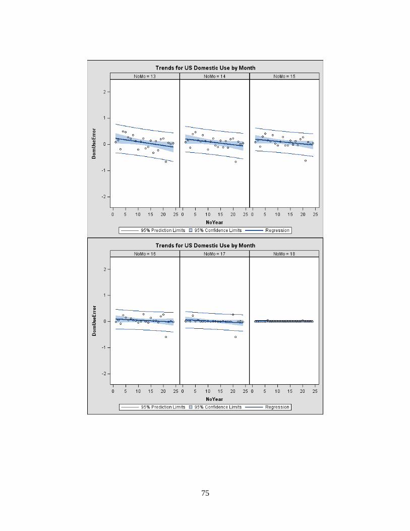
75

76

Appendix C

Regression Plots of the Test of Bias for China Ending Stocks

77

78

79

Appendix D

Regression Plots of the Test of Bias for China Ending Stocks

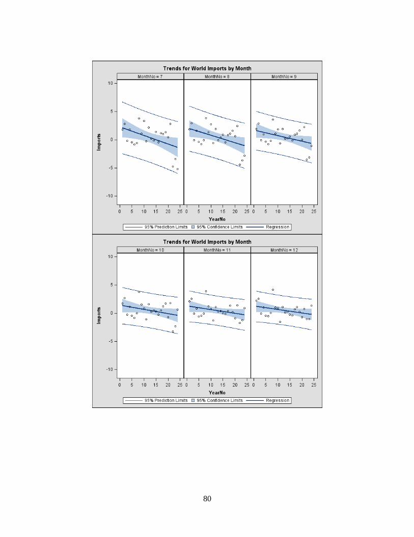
80

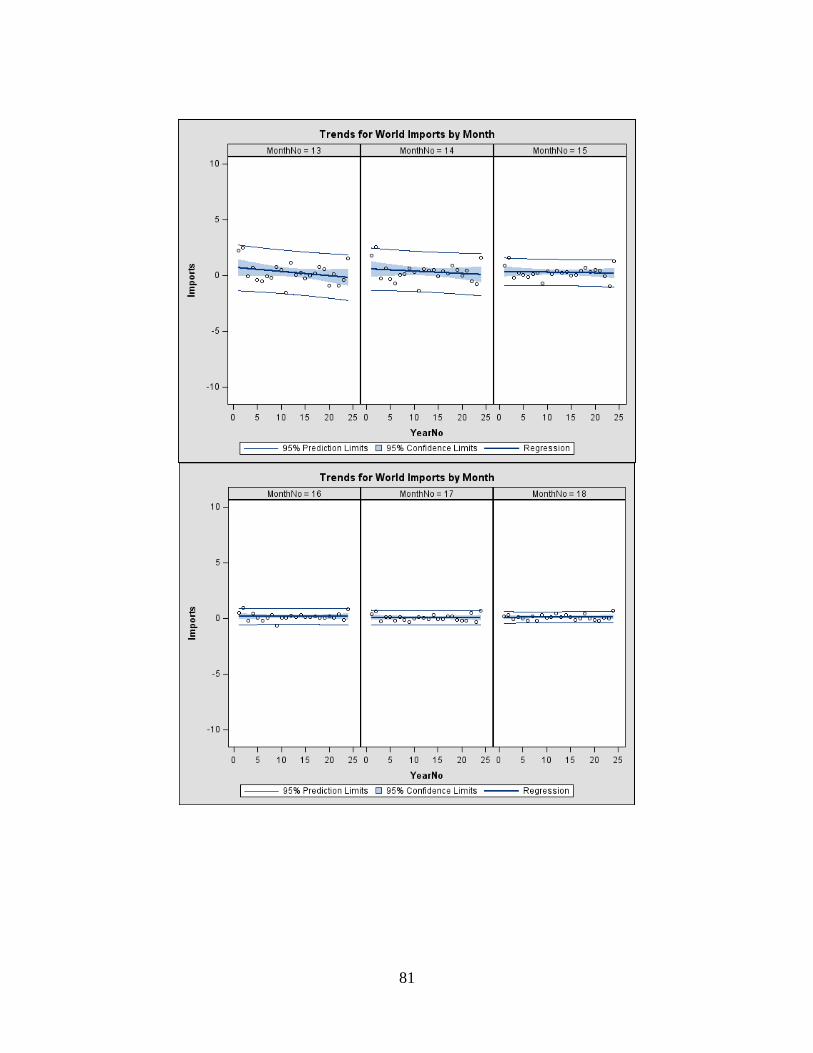
81

82

Appendix E

Chow Test

------------------------------------------- MonthNo=1 -----------------------------------

Structural Change Test

Break

Test Point Num DF Den DF F Value Pr > F

Chow 22 2 20 18.05 <.0001

------------------------------------------- MonthNo=2 -----------------------------------

Structural Change Test

Break

Test Point Num DF Den DF F Value Pr > F

Chow 22 2 20 16.51 <.0001

------------------------------------------- MonthNo=3 -----------------------------------

Structural Change Test

Break

Test Point Num DF Den DF F Value Pr > F

Chow 22 2 20 12.86 0.0003

------------------------------------------- MonthNo=4 -----------------------------------

Structural Change Test

Break

Test Point Num DF Den DF F Value Pr > F

Chow 22 2 20 12.67 0.0003

------------------------------------------- MonthNo=5 -----------------------------------

Structural Change Test

Break

Test Point Num DF Den DF F Value Pr > F

Chow 22 2 20 11.42 0.0005

------------------------------------------- MonthNo=6 -----------------------------------

Structural Change Test

Break

Test Point Num DF Den DF F Value Pr > F

Chow 22 2 20 12.19 0.0003

83

------------------------------------------- MonthNo=7 -----------------------------------

Structural Change Test

Break

Test Point Num DF Den DF F Value Pr > F

Chow 22 2 20 13.29 0.0002

------------------------------------------- MonthNo=8 -----------------------------------

Structural Change Test

Break

Test Point Num DF Den DF F Value Pr > F

Chow 22 2 20 11.76 0.0004

------------------------------------------- MonthNo=9 -----------------------------------

Structural Change Test

Break

Test Point Num DF Den DF F Value Pr > F

Chow 22 2 20 8.41 0.0022

------------------------------------------- MonthNo=10 ----------------------------------

Structural Change Test

Break

Test Point Num DF Den DF F Value Pr > F

Chow 22 2 20 5.36 0.0136

------------------------------------------- MonthNo=11 ----------------------------------

Structural Change Test

Break

Test Point Num DF Den DF F Value Pr > F

Chow 22 2 20 1.66 0.2151

------------------------------------------- MonthNo=12 ----------------------------------

Structural Change Test

Break

Test Point Num DF Den DF F Value Pr > F

Chow 22 2 20 1.06 0.3656

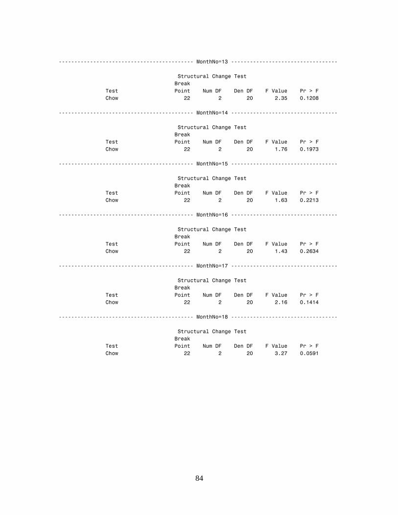
84

------------------------------------------- MonthNo=13 ----------------------------------

Structural Change Test

Break

Test Point Num DF Den DF F Value Pr > F

Chow 22 2 20 2.35 0.1208

------------------------------------------- MonthNo=14 ----------------------------------

Structural Change Test

Break

Test Point Num DF Den DF F Value Pr > F

Chow 22 2 20 1.76 0.1973

------------------------------------------- MonthNo=15 ----------------------------------

Structural Change Test

Break

Test Point Num DF Den DF F Value Pr > F

Chow 22 2 20 1.63 0.2213

------------------------------------------- MonthNo=16 ----------------------------------

Structural Change Test

Break

Test Point Num DF Den DF F Value Pr > F

Chow 22 2 20 1.43 0.2634

------------------------------------------- MonthNo=17 ----------------------------------

Structural Change Test

Break

Test Point Num DF Den DF F Value Pr > F

Chow 22 2 20 2.16 0.1414

------------------------------------------- MonthNo=18 ----------------------------------

Structural Change Test

Break

Test Point Num DF Den DF F Value Pr > F

Chow 22 2 20 3.27 0.0591

85

REFERENCES

Bailey, D.V., and B.W. Brorsen. ―Trends in the Accuracy of USDA Production Forecasts

for Beef and Pork.‖ Journal of Agricultural and Resource Economics 23

(1998): 515–26.

Baltagi, B.H. Econometric Analysis of Panel Data, Second Edition. West Sussex,

England: John Wiley and Sons, 2001.

Baur, R.F., and P.F. Orazem. ―The Rationality and Price Effects of USDA Forecasts of

Oranges.‖ Journal of Finance 49(1994): 681-696.

Botto, A.C., Isengildina, O., S.H. Irwin, D.L. Good. ―Accuracy Trends and Sources of

Forecast Errors in WASDE Balance Sheet Categories for Corn and Soybeans.‖

Selected Paper presented at AAEA 2006 Annual Meetings, Long Beach,

California, July 14-17, 2006.

Colling, P.L., and S.H. Irwin. "The Reaction of Live Hog Futures Prices to USDA Hogs

and Pigs Reports." American Journal of Agricultural Economics 71(1990):84-94.

Dawe, D., ―The changing structure of the world rice market, 1950-2000,‖ Food Policy,

27(4): 355-370. 2002.

Egelkraut, T.M., P. Garcia, S.H. Irwin and D.L. Good. ―An Evaluation of Crop Forecast

Accuracy for Corn and Soybeans: USDA and Private Information Services.‖

Journal of Agricultural and Applied Economics 35(2003): 79-95.

Fortenbery, T. R., and D.A. Sumner. ―The Effects of USDA Reports in Futures and

Options Markets.‖ Journal of Futures Markets 13(1993): 157-173.

Goodwin, B.K., Schnepf, R., and E. Dohlman (2005), Modelling soybean prices in a

changing policy environment, Applied Economics, 37: 253-263.

Goreux, L., A. Plastina, A. Gruere, and Y. Cao. ―The New ICAC Cotton Price

Forecasting Model.‖ Cotton: Review of the World Situation, ICAC,

(July-August 2007).

Gunnelson, G., W. Dobson, and S. Pamperin. ―Analysis of the Accuracy of USDA Crop

Forecasts.‖ American Journal of Agricultural Economics, 54(1972): 639-645.

Harvey, A.C, 1990, The Econometrics Analysis of Time Series. New York: Philip Allan.

86

Irwin, S.H., M.E. Gerlow, and T.R. Liu. "The Forecasting Performance of Livestock

Futures Prices: A Comparison to USDA Expert Predictions." Journal of Futures

Markets, 14(1994): 861-875.

Irwin, S. H., Garcia, H.H., and Good, D.L. ―The Performance of Chicago Board of Trade

Corn, Soybean, and Wheat Futures Contracts after Recent Changes in Speculative

Limits.‖ AAEA 2007 Annual Meeting, July 29-August 1, 2007, Portland, Oregon

Isengildina, O. and S. MacDonald. ―Cotton Prices and the World Cotton Market:

Forecasting and Structural Change.‖ Economic Research Report, Economic

Research Service, U.S. Department of Agriculture, 2009.

Isengildina, O. Irwin, S., and Darrel L. Good. ―Evaluation of USDA Interval Forecasts of

Corn and Soybean Prices,‖ American Journal of Agricultural Economics,

86(2004): 990-1004.

Isengildina, O., S.H. Irwin, and D.L. Good. ―The Value of USDA Situation and Outlook

Information in Livestock and Hogs Markets.‖ Journal of Agricultural and

Resource Economics, 31(2) (2006 a): 262-282.

Isengildina, O., S.H. Irwin, D.L. Good. ―Are Revisions to USDA Crop Production

Forecasts Smoothed?‖ American Journal of Agricultural Economics, 88(4)

(2006 b): 1091-1104.

Just, R. E. and G. C. Rausser. "Commodity Price Forecasting with Large-Scale

Econometric Models and the Futures Market." American Journal of Agricultural

Economics 63(1981):197-208.

Koopman, S. J., A. C. Harvey, J.A. Doornik, and N. Shephard, 2000, STAMP: Structural

Time Series Analyzer, Modeler, and Predictor. London: Timberlake Consultant

Press.

Lence, S., C. Hart, and D. Hayes. ― An Econometric Analysis of the Structure of

Commodity Futures Prices.‖ Poster presented at AAEA 2009 meetings,

Milwaukee, WI, July 25-29, 2009.

MacDonald, Stephen, ―A Preliminary Evaluation of USDA’s Export Forecasts,‖ The 10th

Federal Forecasters Conference 1999: Papers and Proceedings and Selected

Papers of 19th International Symposium on Forecasting, U.S. Department of

Education Office of Educational Research and Improvement, pages 305-316.

MacDonald, Stephen, ―Rational Commodity Forecasts: Improving USDA’s Cotton

Analysis,‖ 12th Federal Forecasters Conference—Papers and Proceedings. 2002,

Veterans Health Administration, U.S. Department of Veterans Affairs, 355-360.

87

MacDonald, Stephen, ―A Comparison of USDA’s Agricultural Export Forecasts with

ARIMA-based Forecasts,‖ 14th Federal Forecasters Conference—Papers and

Proceedings, 2005, Veteran’s Health Administration, U.S. Department of

Veterans Affairs, pages 155-161.

MacDonald, Stephen, ―China’s Cotton Supply and Demand: Issues and Impact on the

World Market.‖ CWS-2007, Economic Research Service, U.S. Department of

Agriculture, November 2007.

Marquardt. R., and A.F. McGann. ―Forecasting Commodity Prices.‖ Commodity Journal,

10 (1975): 29-33.

Meyer, L.A. ―Factors Affecting the US Farm Price of Upland Cotton.‖ Cotton and Wool

Situation and Outlook, CWS-1998, Economic Research Service, U.S. Department

of Agriculture, November 1998, pp. 16-22.

Plato, G., and W. Chambers, (2004). How Does Structural Change in the Global Soybean

Market Affect the U.S. Price? OCS-04D-01, Economic Research Service, U.S.

Department of Agriculture

Ramirez, O. and M.L. Fadiga. ―Forecasting U.S. Agricultural Commodity Prices with

Asymmetric-Error GARCH Models.‖ Journal of Agricultural and Resource Economics,

28, (April 2003): 71-85.

Sanders, D.R., and M.R. Manfredo. ―USDA Production Forecasts for Pork, Beef, and

Broilers: An Evaluation.‖ Journal of Agricultural and Resource Economics

27 (2002): 114–28.

Schaffer, H. ―On predicting the price of corn, 1963-2002,‖ Selected Paper prepared for

presentation at the Southern Agricultural Economics Association Annual Tulsa,

Oklahoma, February 18, 2004

Ticlavilca, A., D. Feuz, and M. McKee. Sparse Bayesian Regression Approach to

Forecast Agricultural Commodity Prices. Poster presented at AAEA 2009

meetings, Milwaukee, WI, July 25-29, 2009.

Timmer, C. P. ―Did Speculation Affect World Rice Prices?‖ Presented at the Rice

Policies in Asia Conference, United Nations Food and Agricultural Organization,

Chiang Mai, Thailand, February 9-12, 2009.

Timmerman, Allan. ―An Evaluation of the World Economic Outlook Forecasts.‖

International Monetary Fund Working Paper. March 2006.

88

Thompson, J.M. ―Analysis of the Accuracy of USDA Hog Farrowings Statistics.‖

American Journal of Agricultural Economics, 34(1974): 1213-1217.

Townsend, T.P. ―This Was a High-Powered Instrument That Sent its Projectile to the

Vitals of the Industry – why USDA Does Not Forecast Cotton Prices.‖

Proceedings of the Cotton Beltwide Conferences. National Cotton Council. 1989.

Westcott, P.C., and L.A. Hoffman. Price Determination for Corn and Wheat: The Role of

Market Factors and Government Programs. Technical Bulletin 1878. Economic

Research Service, U.S. Department of Agriculture (1999).