Evaluating U.S. Fuel Economy Standards In a Model with Producer and Household Heterogeneity

Mark R. Jacobsen*

March 2012

Abstract

This paper employs an empirically estimated model to study the equilibrium effects of an increase in the U.S. corporate average fuel economy (CAFE) standards. A distinguishing feature of the model is that it considers the fact that some firms are unconstrained by CAFE regulation, while others choose either to violate the regulation (pay a fine) or to meet the standard. By taking this heterogeneity into account, I find that the profit impacts of CAFE fall almost entirely on domestic producers. In addition, the model develops utility-consistent welfare analyses that allow direct comparison of the CAFE standard with gasoline taxes, considering the simultaneous household decision of vehicle and miles traveled. Finally, the model accounts for the dynamic effects of CAFE on used vehicle markets – effects that turn out to be important to the welfare impacts. The surplus changes in used car markets make up nearly half of the gross welfare costs of the CAFE standard. These effects fall disproportionately on low-income households. Contrary to previous findings, the overall welfare costs are regressive.

* University of California at San Diego, 9500 Gilman Drive, La Jolla, CA 92093-0508. Email: m3jacobsen@ucsd.edu.

2

1. Introduction

Gasoline use in the United States is associated with considerable external cost, largely

associated with environmental and geopolitical concerns. These include economic and security

risks associated with oil imports as well as the implications of climate change and local air

pollution. Regulation targeted toward the reduction of gasoline consumption was introduced

following the 1973 oil crisis, in the form of the corporate average fuel economy (CAFE)

standards.1 These standards impose a limit on the average fuel economy of the vehicles sold by

a particular company in each year, with separate limits for passenger cars and light duty trucks.

Substantial increases in the stringency of U.S. fuel economy standards have been announced

through 2025, corresponding to the growing salience of concerns associated with gasoline use.2

This paper contributes an empirical examination of the actions automobile producers

take to meet fuel economy standards and measures the welfare cost associated with an increase

in the stringency of CAFE. I examine the mechanisms through which the standards work, and

model distributional implications across both producers and consumers.

A number of prior studies have considered fuel economy standards in the context of

comparing alternative policy instruments: Parry et al. (2007) provide a survey and divide

automobile related externalities into those arising from gasoline use and those from miles

driven, showing that gasoline taxes reduce a greater number of important externalities than do

CAFE standards.3 Furthermore, theory suggests that gasoline taxes are superior to fuel economy

standards even when considering the gasoline externality in isolation. Pricing the externality

1 Important rationales for CAFE regulation in addition to a reduction in gasoline use include protectionism and the correction of market failures in demand for fuel economy. Portney et al. (2003) provide a discussion of the market failure rationale. Goldberg (1998) discusses protection of the domestic automobile industry. 2 Average fuel economy in the U.S. was 27.0 mpg in 2008 (NHTSA [2009]). Current policy requires an increase to 34.1 mpg through 2016 (Environmental Protection Agency and Department of Transportation [2010]), also incorporating an attribute basis which I discuss in Section 6 below. Finally, the Obama administration recently announced an even more ambitious target of 54.5 mpg for model year 2025 (The White House Office of the Press Secretary [2011]). 3 For example fuel economy standards do not directly address automobile accidents or congestion.

3

directly allows more flexibility in that taxes both reduce miles driven and influence vehicle

choice while CAFE standards operate only on the latter channel.4 I offer confirmation that this

ranking holds in my model, but the focus of my paper lies instead with the mechanisms and

distributional implications of CAFE in particular.

This requires explicitly modeling producer behavior under CAFE, building on a

literature focused on producer response to regulation: Austin and Dinan (2005) consider a

representative car producer that faces a regulatory fuel economy constraint. Using demand

elasticities from the literature, they estimate the changes in vehicle fleet that result and consider

surplus changes in the market for new cars. Goldberg (1998) develops an oligopoly model of

producer behavior and considers the implications of CAFE for international trade.5 Kleit (2004)

develops a model based on General Motors’ response to CAFE, modeling pricing behavior.

Similarly, Greene (1991) considers the pricing and fleet mix behavior of U.S. domestic firms in

response to CAFE standards.6

Anderson and Sallee (2011) also consider producer response, but instead of focusing on

prices and fleets they examine a loophole in the regulation. They find evidence that firms have

failed to take full advantage of the loophole in spite of its very low cost. This suggests that the

current standard, at least in recent years with high gasoline prices, may be almost non-binding.7

In contrast, my work centers around a period of low gasoline prices in the late 1990’s where I

find that the regulation substantially influenced firm behavior. The effects I study during this

period therefore allow insight into how producers and consumers may respond to more stringent

regulations like those currently being adopted.

4 CAFE standards may increase miles driven since efficient cars are cheaper to operate. Small and Van Dender (2007) find that this rebound effect can offset 5-10% of the gasoline savings from CAFE. 5 The producer model is based on demand elasticities estimated in Goldberg (1995). 6 Like Austin and Dinan (2005), Greene develops a model to predict the cost of regulation starting from an undistorted state but does not examine empirical producer response directly. 7 Agency problems or market failures within the firm might also account for a failure to take full advantage of the loophole, which involves rewards for the production of flex-fuel vehicles.

4

I address three main challenges unmet in the above literature. First is the treatment of

heterogeneous response across firms, which has been masked by the representative producer

model used in nearly all prior studies. Goldberg (1998) takes an important step, modeling

certain firms as paying the penalties associated with violation. My model includes this group of

fine-paying firms but also encompasses the behavior of a separate, central group including Ford,

GM, and Chrysler: I argue that these firms do not violate the standard or pay any fines, but

instead face a shadow cost in meeting the constraint. In contrast to the literature, I model the

heterogeneous behavior of these firms in a single framework and provide empirical estimates of

shadow cost for firms that choose to just meet the constraint.

A second unmet challenge is the simultaneous measurement of welfare effects across

markets for vehicles and gasoline. The literature on CAFE has generally presented measures of

consumer surplus in individual car markets. Studies of gasoline price sensitivity necessarily

consider utility in gasoline markets as well, but have typically estimated the two demand

equations separately.8 In contrast, I make use of estimates from Bento et al. (2009) to allow

consistent equilibrium welfare analysis across markets.9 I further integrate my model of

producer profits under CAFE, allowing a measure of overall equivalent variation in an

equilibrium setting.

The third main challenge I address concerns the market for used cars. All prior

empirical studies of CAFE to my knowledge have focused on the market for new vehicles, but

regulations influencing new car production necessarily have dynamic effects on used car

markets through time. I model the effects as new cars become used, capturing previously

overlooked welfare implications of a changing used car fleet.

8 For example Goldberg (1995) and West (2004) estimate demand for vehicles and gasoline separately, correcting for the simultaneity with the technique introduced by Dubin and McFadden. 9 The demand equation for miles is derived using Roy’s identity and the conditional indirect utility function describing vehicle choice. A single set of utility parameters results that can be used to derive a measure of equivalent variation.

5

My results reflect these innovations. I examine the effects of CAFE at the manufacturer

level and find that almost all profit impacts of the current standard are felt by domestic firms. A

key mechanism behind this result is substitution in the market for large, high-horsepower

vehicles: When domestic firms cut production of these vehicles in order to meet the standard,

the unconstrained and fine-paying firms will increase production in their place. The substitution

pattern protects fine-paying firms from profit impacts and also harms the efficacy of CAFE in

reducing gasoline use.10 Important policy steps toward a harmonized standard may be able to

mitigate this effect.

At the aggregate level, I find that a 1 mile-per-gallon increment to the stringency of

CAFE reduces long run gasoline use by 3%. Short run effects are much smaller, demonstrating

the significance of explicitly modeling the gradual penetration of fuel economy standards

through the used car fleet. I find that the aggregate welfare costs associated with these gasoline

savings are three to six times larger for a CAFE standard than a comparable gasoline tax.11

Finally, one of my more striking conclusions is that the progressivity of a CAFE

standard can be overturned by long run effects in the used car market. The initially progressive

aspect of the standard is intuitive and confirmed here: wealthier households tend to buy more

new vehicles, and thus bear much of the initial burden. I find, however, that changes in used car

prices over time and long run shifts in the composition of the used car fleet eventually

overwhelm this, making the total effect regressive. Prior studies of fuel economy regulation

have overlooked this result with their focus on new car markets and a representative consumer.

The rest of the paper is organized as follows. Section 2 describes the CAFE regulation

and introduces the model. Section 3 demonstrates the importance of firm heterogeneity and

categorizes firms empirically. Section 4 describes an estimation procedure using first order

10 The degree of imperfect substitution in the luxury vehicle market controls the extent to which gains in domestic average fuel economy are offset. 11 Austin and Dinan (2005) is the only study to my knowledge to offer comparable estimates. They approximate consumer surplus changes using new car and gasoline demand elasticities but do not include used car markets or integrate demands in a utility framework. They find that gasoline taxes have 60 to 70% less distortionary cost than an equivalent CAFE standard.

6

conditions on firm behavior. Section 5 offers an alternative source of evidence for firm pricing

behavior. The welfare and distributional impacts of a change in CAFE policy are measured in

Section 6 using the estimated parameters. Conclusions are offered in Section 7.

2. Regulation and Model of Producer Behavior

a. Fuel Economy Regulation

CAFE standards are enforced at the level of a manufacturer’s fleet of new vehicles in a

given model year. Each manufacturer’s production is divided into two separately regulated

fleets: passenger cars and light duty trucks.12 The regulation defines a firm’s corporate average

fuel economy, for each of the two fleets, as:

CAFEfleet =qj

j∈fleet∑

qjmpgjj∈fleet

∑ (1)

where qj is the quantity of model j produced and sold by the firm and mpgj is that model’s fuel

economy measured in miles-per-gallon.13 New rules beginning in 2012 modify this formula to

include an attribute of the vehicle (the area between its wheels, or "footprint") in determining the

overall limit: I explore the effect of this change in the simulations of Section 6.

The passenger car standard was held constant at 27.5 mpg for every year between 1990

and 2010. The light truck standard has increased gradually over time but, convenient for my

analysis, was held fixed at 20.7 mpg in all years between 1996 and 2004. The rules allow for

the banking of “credits,” defined in terms of quantity weighted deviations from the standard, for

12 The regulation subdivides the passenger car fleet into those produced more and less than 75% domestically. While this division may have had some impact initially, firms have since been able to equalize the fuel economy of the two groups of passenger cars without major structural changes (NRC, 2002). The ease of moving cars above and below the “import” threshold and the lack of complete data on the fraction of domestic parts in each vehicle lead me to consider passenger cars as a single group. 13 The distinction between production and sales can be abstracted from due to the marketing of vehicles by model year: Dealers have strong incentives to avoid holding vehicles from the previous model year after the new generation is released.

7

up to three years. For example, if the firm’s car fleet has a fuel economy of 28.5 mpg it

accumulates credit that can be used to offset a 26.5 mpg fleet in any of the next three years.14

Similarly, the firm may borrow against future credits, as long as it repays the debt within three

years. If the firm fails to repay a debt within three years it is found in violation of the regulation

and assessed a fine of $50 for each mile per gallon below the standard multiplied by the total

number of vehicles in the fleet. The fine was increased to $55 after the end of my sample

period.

The banking and borrowing scheme produces a complex set of dynamic incentives for

the firm. In particular, it can be shown that a decision made in the current period can affect the

firm in all future periods and conversely that a firm’s regulatory compliance status in the current

period can depend on the entire history. This is demonstrated in Appendix B. The dynamic

features of the regulation generate small amounts of variation in the stringency of the standard

through time. Section 5 exploits the details of this variation to test my basic assumption on the

pricing behavior of producers. The results from my main model will be static: This abstracts

from the three-year banking and borrowing provision, but I argue provides a good

approximation of shadow cost when pooling data over a period of stable demand and prices

(1997-2001 in the primary specification). Further discussion is again provided in Appendix B.

b. Model of Producer Behavior

Automobile producers are assumed to be oligopolists in a differentiated products market

and equilibrium is defined as a set of prices such that each firm is maximizing profits given the

actions of all others.15 Firms are treated consistently in that heterogeneity enters only through

parameters. The maximization problem specified here is written in terms of an individual firm

conditional on the behavior of its competitors.

14 The example assumes that the overall sales of the firm are the same in the two years, since the number of credits earned is weighted by quantity. 15 The prices of other firms enter through residual demand. All else equal, an increase in the price of a car by one firm shifts the residual demand faced by other firms outward.

8

Introducing CAFE regulation into the firm’s profit function involves modeling the cost

associated with a violation of the standards. I will assume that this cost comes from two

sources: The first is the fine levied by the regulator, which varies linearly with the degree of

violation. The second is a fixed cost of violation, encompassing the legal, political, and

corporate image losses also resulting from infractions.

Avenues for compliance with CAFE regulation will be balanced against the costs of a

violation. Compliance involves selling more high-efficiency vehicles (and fewer low-efficiency

ones) as a fraction of the total, which I capture through the firm’s choice of price in a Bertrand

setting. In the long-run, firms will also invest in new technologies.16 I do not estimate a

technological frontier directly in the model, but am able to consider the role of technology in an

extension to the overall welfare analysis.17

With these components I model each firm as maximizing profit net of the costs of

violation, solving:

max{ pj , j∈J}

(pj − cj )qj (P)j∈J∑

⎛

⎝⎜⎞

⎠⎟− I(Qi ) Hi + FC (Qi ) + FT (Qi )( )⎡

⎣⎢⎢

⎤

⎦⎥⎥

(2)

where pj, cj, and qj are respectively the price, cost, and quantity of a particular model j made by

firm i. J is the set of all cars made my firm i. P is the vector of prices of all cars in the market,

and Qi refers to the quantities of all models manufactured by firm i. I is an indicator function

taking the value of 1 if the firm is in violation of the standard and 0 otherwise. The functions FC

and FT represent the fines faced for the car and truck fleets respectively. Hi represents the firm-

specific component of cost that is fixed conditional on violation.

16 Klier and Linn (2008) consider the question of technology and fuel economy standards, examining a “medium-run” case where technology enters with an intermediate scope. 17 My extension of the model to include technology follows Austin and Dinan (2005). The extension relies on the general result that cost-minimizing firms equalize the marginal costs of compliance across available channels. For an explanation in the specific context of fuel economy see Anderson and Sallee (2011).

9

The level of the fines depends on fleet size and deviation from the standard. I use the

functional form directly from the regulation, which is administered by the National Highway

Traffic Safety Administration (NHTSA):

FC (Qi ) = qj (P)j∈carfleet∑

⎛

⎝⎜⎞

⎠⎟⋅50 ⋅ dcarfleet − CAFEcarfleet( )

FT (Qi ) = qj (P)j∈truckfleet∑

⎛

⎝⎜⎞

⎠⎟⋅50 ⋅ dtruckfleet − CAFEtruckfleet( )

(3)

where dcarfleet is the level of the standard for the manufacturer’s car fleet, 27.5 miles per gallon,

and CAFEcarfleet the corporate average fuel economy for the firm’s car fleet as defined in (1).

Note that fleet fuel economy is computed as the harmonic mean in order to match the NHTSA

rule precisely. The expression for the light duty truck fleet, FT, is analogous with the standard

fixed at 20.7 in 2001.

The firm level fixed components of cost, Hi, represent other losses that are incurred

when violating the regulation.18 Corporate public image and legal liability for environmental

damage may be important factors. A firm’s political capital, valuable in times of financial

distress or when negotiating stringency of regulation, could also be eroded by violations.

Allowing the magnitude of these costs to vary across firms is important: Foreign companies

may have less exposure to U.S. environmental lawsuits or less need for U.S. political capital.

Similarly, firms that specialize in high performance cars may be less averse to a reputation for

environmental violations than are full-line automakers.

These costs are difficult to measure directly, so in working with the model I must rely on

two key assumptions to bound Hi: i) For firms that have complied historically the costs in Hi are

at least large enough to justify their decision. ii) For firms regularly found in violation of the

standard the costs are small enough that the violation is consistent with profit maximization.

18 Some of these costs may be argued to vary with the severity of violation. The distinction is irrelevant for the purposes of estimating the shadow cost of firms never observed to violate the standard. It could, however, somewhat influence the group of firms observed to violate since they must weigh the degree to which they fall below the standard.

10

A final important simplification is that the indicator for violations, I, is defined for a

single year in a static version of the problem whereas the regulation in fact allows banking and

borrowing of credits. A dynamic model, as shown in Appendix B, involves optimization over

all years simultaneously with a state space depending on the firm’s entire history.19 The

approximation to require compliance in a single year both provides a tractable model and is

consistent with a dynamically optimizing firm’s behavior in a period of stable demand with

convex costs of compliance.20

Solving for Firm Behavior

Equation (2) can be divided into three cases, depending on the state of the indicator I. In

the first case, I is equal to 0 at the unconstrained optimum shown below. In other words, if the

firm maximizes profits without regard to I it will already meet or exceed the standard. The

maximization problem in (2) can then be reduced to a standard multi-product profit

maximization problem subject to the residual demand curves given by the qj’s:

max{ pj , j∈J}

(pj − cj )qj (P)j∈J∑

⎛

⎝⎜⎞

⎠⎟ (4)

In the second case, the maximum in (2) is reached when I is equal to 1. Profits are

maximized when the firm is violating the standard and paying all associated costs. After

replacing I and eliminating constant terms (2) reduces to:

19 It may seem that compliance state could be determined via a moving set of seven-year windows, an already difficult intertemporal problem, but in fact the accounting of credits and debits can lead to dependence on the entire history. 20 Convexity of compliance costs (which follows from standard assumptions on the multi-product demand system) causes the cost of repaying borrowed credits to exceed the initial gain. Note also that this is absent discounting: In a model that permits borrowing, a firm would like to borrow in the early years of the regulation and pay back late, letting the value of the permits rise with the discount rate. In the case of CAFE, however, the three-year limit on borrowing mitigates the importance of this effect.

11

max{ pj , j∈J}

(pj − cj )qj (P)j∈J∑

⎛

⎝⎜⎞

⎠⎟− FC (Qi ) + FT (Qi )

⎡

⎣⎢⎢

⎤

⎦⎥⎥

(5)

In the third case, the maximum in (2) is reached when the firm is just complying with the

standard. In other words, I is equal to 0 but any small reduction in fuel economy would cause

the firm to violate the standard. The solution to (2) for a constrained firm can be written as the

maximization:

max{ pj , j∈J}

(pj − cj )qj (P)j∈J∑

⎛

⎝⎜⎞

⎠⎟

s.t.

qj (P)j∈carfleet∑

qj (P)mpgjj∈carfleet

∑− dcarfleet ≥ 0 and

qj (P)j∈truckfleet∑

qj (P)mpgjj∈truckfleet

∑− dtruckfleet ≥ 0

(6)

where the constraint above is the definition of I(Qi ) = 0 . For economy of notation I have

omitted the case where a firm may be constrained in one fleet but not the other, although this

possibility is considered in both the estimation and policy simulations.

The first order conditions for each of these three cases are written out explicitly in

Section 4 as estimation equations.

3. Heterogeneous Response to CAFE: Three Types of Firms

I develop a dataset and metric to examine the division of major automakers into the three

categories identified by the theoretical model above. The analysis is based on historical

response to CAFE and my definitions of the groups below are followed by two proposed metrics

for categorizing firms.21 In contrast to Goldberg (1998), I not only consider firms that are

affected by the CAFE fines, but also firms that are constrained by the regulation. I will find that

this new group of constrained firms bears much of the burden of policy and influences the

efficiency of the regulation. 21 Given enough variation through time, firms may have moved from one category to another, but this does not appear to have been the case for the major producers in the U.S. market.

12

Groups

I. The first group consists of those firms whose car and truck fleets exceed the standard.

More precisely, given the set of prices and vehicles offered by other makers, the profit-

maximizing quantity for each model results in a fleet of new vehicles that is unconstrained by

the regulation. Toyota and Honda are the two largest firms in this category; their car and truck

fleets have well surpassed the standard every year since 1978. This group corresponds to

equation (4) above.

II. The second group is comprised of firms that violate the standard and pay the associated

fines. BMW and Mercedes (until its merger with Chrysler) are the two largest firms in this

group. They have both violated the standard for each model year since 1987 and have paid

about $500 million in fines as a result. They correspond to equation (5) above.

III. The third, and arguably most important, category consists of firms that are constrained

by CAFE as modeled in equation (6). These are firms that, in the absence of regulation, would

choose to produce a fleet that falls below the CAFE standard, but alter their fleet such that it just

meets the standard when regulation is introduced. Implicitly, this means that total costs

associated with violating the standard are larger than the forgone profits from compliance. I

show below that the traditional “big three” producers, Ford, GM, and Chrysler, fall into this

category.

CAFE compliance status for each firm is calculated annually and available from the

NHTSA.22 Figure 1 plots the raw data for one firm in each category: The behavior of Toyota

and BMW is clear, with Toyota exceeding and BMW violating the standard in every year. Ford,

while not meeting the standard exactly in any one year, appears constrained in the sense that

through time its deviations from the standard almost precisely cancel. In other words, the

credits that it earns from a year when it is slightly above the standard are offset almost exactly

22 National Highway Traffic Safety Administration (2009) and (2010).

13

by years when it falls below the standard. Figure 2 plots the history of the largest firms in each

category, as divided by the metric below.

To incorporate the dynamic nature of the regulation, where credits from over-compliance

may be used on a one-to-one basis to offset under-compliance, I aggregate firm deviations from

the CAFE standard through time. This is done in Table 1 for the largest firms. In the left hand

(car fleet) panel, the row for Honda, for example, indicates that during the period 1990-2001 the

firm produced a fleet that exceeded the CAFE standard by an average of 3.96 miles per gallon.

Mercedes, on the other hand, produced a fleet whose fuel economy averaged 3.29 miles per

gallon below the standard, paying penalties for violating the regulation in almost every year.

Ford, GM, and Chrysler have aggregate deviations very close to zero – measuring less than 0.2

miles per gallon above the standard. This places them in the third group, firms that are

constrained by the standard but not found in violation.23

To further emphasize the differences in the three groups, the table also shows the

fraction of years in which the firm had a fleet fuel economy that fell below the standard. Notice

that the firms in the violating group were below the standard in every year, while the

unconstrained firms are above in almost every year. The constrained domestic firms spend

some years under the standard, and some years over, using credits from the good years to offset

under-compliance in the bad years.

The second panel repeats this exercise for the separately regulated light duty truck fleet.

The same group of three domestic firms is in the constrained section, with the fleets of the

largest truck makers, GM and Ford, again averaging less than 0.1 miles per gallon above the

standard.24

23 Since I begin the calculation in 1990 (after the level of the standard was fully stabilized) the slight over-compliance measured may capture the repayment of credits owed from the late 1980’s. 24 The truck fleets of VW, Isuzu, and Mitsubishi are not differentiated as sharply by the second metric, so I place these smaller firms according to their average performance, which in all cases coincides with performance in the central 1997-2001 period I consider. Volkswagen violated the standard in each year since 1996 and was forced to pay a fine on all of its 1997-2001 truck fleets. Isuzu and Mitsubishi both had fleets well above the standard in this period, and did not pay fines.

14

4. Data and Estimation

In order to develop a more complete understanding of automobile markets in the context

of CAFE regulation, models of both the demand and supply of automobiles are integrated.

Automobile demand follows Bento et al. (2009), and supply is given by the model described in

Section 2. The pair of models has the advantage of consistency in the sense that I employ the

same data sources and assumptions throughout. In brief, the household level results from Bento

et al., described in the first subsection below, are used to derive a set of residual demand curves

faced by producers and to allow measurement of welfare effects.

The second subsection below describes estimation of the producer model. The

computations for the unconstrained and fine-paying cases follow Goldberg (1998). The

constrained case, for Ford, GM, and Chrysler, provides a new challenge in separately estimating

the shadow costs of the regulation. The first order conditions of the profit-maximization

problems above are employed in estimation. The estimates provide a producer level

understanding of responses to fuel economy regulation.

a. Household Demand

Demand follows Bento et al. (2009). The primary data source is the 2001 National

Household Travel Survey (NHTS), which provides, in addition to demographic indicators,

household level survey data on automobiles owned and vehicle miles traveled (VMT). The

vehicle data for both the demand and supply side are divided into the following 10 vehicle

classes, 5 age categories, and 7 manufacturers:

Classes Age categories Manufacturers Compact New cars Ford Luxury compact 1-2 years old Chrysler Midsize 3-6 years old General Motors Fullsize 7-11 years old Honda Luxury mid/fullsize 12-18 years old Toyota Small SUV Other Asian Large SUV European Small truck Large truck Minivan

15

Vehicle characteristics come from Ward’s Automotive Yearbook, and prices from the

National Automobile Dealer’s Association (NADA) Car Guide. An annual measure of vehicle

rental cost based on the change in resale value, registration, and insurance costs is constructed

and given in the model below by rhj . Fuel economy and local prices of gasoline are used to

compute a measure of per-mile operating cost for each household and vehicle, phjM .25 (The ~

symbol throughout indicates data and parameters estimated within the household problem.)

The key advantages of this demand model in my application to CAFE standards are i)

the simultaneous estimation of the choice of vehicle and miles driven and ii) the model of

demand for used vehicles. This represents an important improvement over previous work, much

of which has employed a two step procedure and has not considered the used market.26 The

single set of parameter estimates, obtained by using the information in both the vehicle choice

and VMT data, allows the numerical simulation of an integrated set of household decisions and

consistent measurement of welfare effects under policy scenarios.

Specifically, indirect utility for household h conditional on the discrete choice of vehicle

j is given by:

Vhtj =Vhj' + µhεhtj

Vhj' = −1λh

exp − λh

yh / Th − rhj

phx

⎛

⎝⎜

⎞

⎠⎟

⎛

⎝⎜

⎞

⎠⎟ −

1βhj

exp α hj +βhj

phjM

phx

⎛

⎝⎜

⎞

⎠⎟ + τ hj

(7)

where yh is household h’s income and phx the price of the outside good. The utility parameters

λh , αhj , βhj , and τ hj are to be estimated. Subscript t indicates the choice occasion for households

purchasing multiple vehicles, see full article for an in depth discussion of this component. The

random component of utility, given by µhεhtj , is drawn from the type I extreme value

25 phjM also includes a measure of per-mile maintenance costs and the portion of insurance costs that vary

with annual mileage. 26 For example, West (2004), Goldberg (1998) and Train (1986) use a two-step procedure to sequentially estimate the discrete choice of vehicle and the demand for VMT.

16

distribution, with the probability of a given discrete choice j maximizing utility therefore taking

the logit form:

Prht ( j) =exp(Vhj

' / µh )

exp(Vhk' / µh )

k∈Ω∑

(8)

where Ω represents the set of all new and used vehicles in the market.

The second equation, for the continuous choice, is derived directly from the indirect

utility function in (7) using Roy’s identity, and is given by:

Mhtj = exp α hj +βhj

phjM

phx

⎛

⎝⎜

⎞

⎠⎟ + λh

yh / Th − rhj

phx

⎛

⎝⎜

⎞

⎠⎟

⎛

⎝⎜⎜

⎞

⎠⎟⎟

(9)

where Mhtj is miles driven for household h conditional on choosing vehicle j. We assume

Mhtj

is measured imperfectly, yielding the estimation equation, M̂htj = Mhtj +ηhtj , where

M̂htj is the

observed survey response on miles driven and ηhtj is i.i.d. Gaussian error.

To compute the estimates, we adopt a Bayesian approach and use a variation of Allenby

and Lenk’s implementation of the Gibbs sampler. Mean values for the elasticities of miles

driven with respect to operating cost and income, respectively, are found to be -0.69 and 0.62,

with the elasticity of demand for gasoline estimated to be -0.32. Mean demand elasticities for

new vehicles are estimated to be -2.0. The utility parameters are allowed to vary by household

income, family composition, education, MSA size, and race. These sources of variation allow a

particularly detailed view of the distributional effects of policy.

The estimates from the demand model are driven by cross-sectional variation in gasoline

prices and the relative ownership costs of vehicles.27 The demand model fits the data quite

closely, particularly for VMT where predicted and actual mileage differ by less than 1% across

income quartiles. The fit here is important for the present paper, where I wish to examine the

27 Gasoline prices varied by 56% across metropolitan areas, while cost of living differences (a factor of 1.77 across areas in our sample) and state-level variation in insurance, registration, and maintenance costs produce variation in the effective rental price of vehicles.

17

effects of policy along the income dimension. Used car ownership by income group, also

important in the analysis, is similarly closely predicted. My simulation model begins by exactly

replicating the car ownership and driving patterns predicted by the demand model, and then

letting them change as the policy moves equilibrium prices.

The relative magnitudes of the gasoline price elasticity and the vehicle choice elasticities

above are important for the overall welfare estimates that I present in simulation. For this

reason, I explore the sensitivity of my results to changes in these elasticities in Section 6d: The

wedge in cost between the gasoline tax and the CAFE standard is sensitive to elasticities in an

intuitive way, while my findings on the heterogeneous impacts across producers and income

groups remain robust.

b. Producer Costs

Estimation of cost parameters determining producer response to CAFE regulation

represents the final step in using the pair of models for policy analysis. In order to recover the

cost parameters I make use of the firms’ first order conditions drawn from the model of behavior

in Section 2. Where the residual demand functions enter I incorporate estimates from the

household demand system just discussed. We will see that an estimate of costs may be

computed directly, along the lines of Goldberg (1998), for two of the three groups of firms:

those that are unconstrained or that are paying the fine. For the third class, the constrained

domestic firms, I introduce an econometric model to separate two components of cost under a

pre-existing CAFE standard: marginal production cost, and the shadow cost of existing

regulation.

i. Computation for Unconstrained and Fine-Paying Firms

First consider the case of the unconstrained firm given in equation (4). This is a standard

multi-product profit maximization problem and the set of first order conditions with respect to

price may be written in matrix notation as:

18

Qi (P) + Di ⋅ (Pi − Ci ) = 0 (10)

where Qi is the vector of quantities of each type of vehicle made by firm i, and Pi and Ci the

corresponding price and cost vectors. Di is the j by j matrix of derivatives of demand where the

k, th element of Di is: ∂q ∂pk . I compute the matrix Di from the aggregate household

demand system, and the vectors Qi and Pi are data. An estimate of costs may then be computed

directly from (10).

In the second case, which describes firms observed to be violating the standard and

paying the fine, the first order conditions may be written as:

Qi +Qi *GiC +Qi *GiT + Di ⋅ (Pi − Ci − F̂iC − F̂iT ) = 0 (11)

where F̂iC and F̂iT are vectors with the elements defined as the per-vehicle fine for each car and

light duty truck. The vectors GiC and GiT are the derivatives of F̂iC and F̂iT with respect to

vehicle price.28 As mentioned, this calculation and the one above for unconstrained firms so far

follow the analysis done in Goldberg (1998), with the exception that I model the average fuel

economy calculation using the regulation’s harmonic mean formula rather than a linear average.

The result is that the derivatives in GiC and GiT are no longer linear, but are given by:

GiC[ ]k ≡∂F̂iC∂pk

= 50 ⋅

∂qj∂pkj

∑qjmpgjj

∑−

qj ⋅j∑ ∂qj

∂pk1

mpgj

⎛

⎝⎜⎞

⎠⎟j∑

qjmpgjj

∑⎛

⎝⎜⎞

⎠⎟

2

⎡

⎣

⎢⎢⎢⎢⎢

⎤

⎦

⎥⎥⎥⎥⎥

(12)

Despite the complexity of this expression, an estimate of Ci can still be computed directly from

the data as in the unconstrained case.

ii. Estimation Procedure for Constrained Firms

The largest domestic automakers fall into neither of the two categories described by

Goldberg, but instead are constrained by CAFE. The model given in (6) above is able to capture 28 The * symbol in (11) indicates element-by-element multiplication.

19

the incentives for all three types of firms, including this case where the regulation just binds. I

estimate the shadow cost of the regulatory constraint as follows:

For ease of notation, first rewrite the maximization problem given in (6) in vector form:

maxPi

Qi' (P) ⋅ (Pi − Ci )⎡⎣ ⎤⎦

subject toQi

' (P) ⋅ LiC > 0 and Qi' (P) ⋅ LiT > 0

(13)

where the k-th element of LiC is 1− 27.5mpgk

⎡

⎣⎢

⎤

⎦⎥ for passenger cars and 0 otherwise. The k-th

element of LiT is 1− 20.7mpgk

⎡

⎣⎢

⎤

⎦⎥ for light duty trucks and 0 otherwise. We can then write the first

order condition with respect to price of the associated Lagrangian as:

Qi (P) + Di ⋅ (Pi − Ci + λiCLiC + λiT LiT ) = 0 (14)

where λiC and λiT are the scalar Lagrange multipliers for firm i associated with the passenger

car and light duty truck constraints, respectively. In the previous two cases we saw that an

estimate of Ci could be computed directly from the first order conditions. This is no longer

possible since the terms representing the shadow cost of CAFE are also unknown. The

remainder of this section describes an econometric approach for estimating λiC andλiT , from

which the remaining parameters needed for the policy simulations may be computed.

Notice that, at the optimum, λiC (and similarlyλiT ) takes the same value across all

models produced by a given manufacturer. This approach closely parallels Goldberg's (1995)

estimation of the shadow cost of the Vehicle Export Restraint, where again the key restriction is

that the shadow cost of the regulation will be made equal across the vehicles a firm produces.

Intuitively, the model will measure the portion of the markup that varies with fuel economy after

controlling for the expected markup based on the demand elasticity. The farther below (above)

the standard a vehicle's MPG rating is the greater (lower) is the markup we expect to be placed

on that vehicle all else equal. LiC and LiT represent this distance, taking positive values for

relatively efficient vehicles and negative values for inefficient ones.

20

While I do not observe the total markup (i.e. the combination of dealer and manufacturer

markups) I do have data on the dealer's portion of the markup in the form of the retail and

invoice price for each vehicle. Bresnahan and Reiss (1985) develop a model of successive

monopoly in vehicle sales arguing that the dealer markup will be proportional to the

manufacturer markup. They estimate that the ratio of markups is constant at 0.71 across models,

meaning that as total markup increases (for example markups are typically higher for luxury

vehicles) the dealer and the manufacturer continue to split it in the same proportion. I employ

this in constructing a proxy for the total markup, appearing as Bi in the equations below.29

Specification (I) in (15) below uses the proxy directly, adopting the 0.71 ratio in markups

allowing only an additive fixed effect by make. It is important to note, however, that the

Bresnahan and Reiss estimates are more than two decades old and the split in markups may have

changed substantially. This prompts my specification (II), allowing an arbitrary ratio of dealer

and manufacturer markups specific to each firm. (II) therefore imposes only the theoretical

restriction from the earlier paper, that the ratio between dealer and manufacturer is fixed across

vehicle models within the firm:

(I) Bi = Pi − Ci +α i + εi(II) Bi = γ i ⋅ (Pi − Ci +α i + εi )

(15)

In specification (I) α i is an additive constant, Pi − Ci the overall price-cost margin, and

εi is measurement error independent of the variables entering the producer’s optimization

problem. Specification (II) adds a multiplicative term that may vary by firm, γ i , and is

preferred since it both relaxes the strict link to Bresnahan and Reiss and further allows the

markup ratio to differ flexibly across makes. I show that the central parameter estimates of the

model are robust across both specifications, but find that model (II) fits the data somewhat more

closely.

29 Specifically, the 0.71 ratio implies that the total price-cost margin is 2.4 times the observed dealer margin.

21

Rearranging the first order condition in (14), we can rewrite the optimal price-cost

margin in terms of the demand system and the shadow costs of CAFE:

Pi − Ci = −Di

−1Qi (P) − λiCLiC − λiT LiT (16)

Combining (16) with the functional forms considered for Bi in (15) yields the following two

models:

(I) Bi = −D

i

−1Qi (P) − λiCLiC − λiT LiT +α i + εi(II) Bi = γ i ⋅ (−Di

−1Qi (P) − λiCLiC − λiT LiT +α i + εi ) (17)

The parameters, λiC , λiT , α i and γ i , are estimated by least squares. The intuition may

be clearest in the linear specification (I) where we construct a residual markup (that is, the part

of the markup that cannot be explained by optimization with respect to the demand system) and

regress it on the LiT and LiC terms. The shadow costs λ will differ from zero when the distance

between a particular vehicle's fuel economy and the standard systematically captures the

unexplained portion of markup. The independence of the error and Li (fuel economy) is

therefore the main identifying assumption. A placebo test in the Appendix (Table A1) using

unconstrained manufacturers suggests that there is not a general, spurious correlation between

the error and fuel economy in (17): λ for unconstrained firms appears indistinguishable from

zero.

The central results of estimation for constrained producers are presented in Table 2.

Model I is estimated first using a scalar value α i and then allowing it to vary for each make-

fleet combination. Similarly, model II is first estimated with scalar values for α i and γ i and

then more flexibly allowing γ i to vary with make-fleet combination. While the models are both

identified in cross-section, data for the years 1997-2001 is pooled due to the limited number of

observations available for a single year. Implicitly, this adds the assumption of a constant

shadow cost of CAFE across these five years. Recall, however, that firms can shift the CAFE

22

requirements across time, so that in a period of stable demand it is not unreasonable to assume

that they are able to equalize the shadow costs.30

The estimates for λiC and λiT shown in Table 2 are similar across specifications and

vary significantly among manufacturers. Perhaps not surprisingly, the models with fixed effects

by make-fleet fit the data considerably better. To attach economic meaning to the parameters

and the differences observed among firms, I compute the marginal effects of a unit change (one

mile per gallon) in the standard on the profits of each firm and fleet in Table 3.31 In this table,

and as the central case in the policy simulations, the values from model (IIb) are used.

Appendix A demonstrates the robustness of the results to alternative specifications of the fixed

effects, the inclusion of year fixed effects and the placebo test on unconstrained firms.

The highest shadow costs displayed in Table 3 are for GM’s passenger car fleet.

Intuitively, this fleet is estimated to be the most constrained in the sense that the pricing of

component vehicle models reflects the largest distortions attributable to regulation.32 At the

other end of the spectrum, Ford’s car fleet shows the smallest effects from CAFE. These

estimates are consistent with casual observation in the domestic auto industry: among

carmakers, Ford has a reputation for its “practical” car line (Taurus, Escort, Focus) whereas GM

is best known for a lineup of larger, high-horsepower vehicles with correspondingly low fuel

economy. In truck fleets, Ford and GM are similar, while Chrysler, with its dominance in the

30 The seven-year limit on the window of banking and borrowing and long run changes in market conditions may mean that firms either can not or do not wish to equalize shadow costs over long time horizons. In order to limit the impact of these long run effects, I restrict the time period for estimation to the five years leading up to 2001 — the year from which the cross-section of household demand data is drawn. Note also the stability of the CAFE standard through this time period (see Section 2a). 31 The marginal effects are derived by inverting the (nonlinear) transformation performed on the constraint in equation (13). Further dividing by the quantity of vehicles sold results in a form roughly comparable to that in Anderson and Sallee (2011). The higher values here (several hundred dollars per car compared with less than 20) result in part from the greater effective stringency of a standard when fuel prices are low ($1.45 / gallon in my sample). Simulating the shadow cost of the existing standard at $3.50 / gallon results in Ford cars and GM light trucks becoming completely unconstrained (zero shadow cost), with costs for the other makes reduced more than 50%. 32 The distortions exceed the $50 fine for violation, suggesting that domestic automakers have substantial profit motives for compliance in addition to the nominal fines imposed for violation. See discussion in Section 2b.

23

minivan market, has the lowest marginal costs of CAFE. (Minivans have significantly better

fuel economy than most SUVs.)

5. Time Series Model of Prices

The analytical model and parameter estimates above are based on the assumption that

firms react to CAFE by changing prices, thereby affecting demand and the composition of their

fleet in a process known as "mix-shifting." It is possible to test this assumption by exploiting

small amounts of time series variation in the stringency of CAFE standards at the firm level.

The estimation strategy uses a firm’s history of compliance, and therefore information

about how many extra credits it has or obligations it owes, to derive a proxy for how constrained

it is in any given year. Price is regressed on the information about CAFE status to assess how

firms alter prices based on the regulation. While this model makes a very different set of

assumptions and uses different data sources, it results in a set of estimates consistent with the

central results presented in Section 4b.

Recall that the regulation allows both banking credits for three years and borrowing

against three years worth of future credits. If the firm holds credits longer than three years they

expire, and if it fails to repay borrowed credits within three years the firm is found in violation.

The first simple measure of annual “firm state” I construct is simply the number of credits a firm

has that will expire if they go unused minus the number of borrowed credits it must repay to

avoid penalty. A positive value means that a firm may freely produce a fleet that is less than the

standard, so that the firm is less constrained by the regulation. A negative value means that a

firm must exceed the standard in order to avoid a penalty for not paying back borrowed credits,

and is therefore more constrained by the regulation.

I construct this measure from my dataset as follows. Define the variables:

δ0,t ≡ Credits (debts) expiring (due) in year tδ1,t ≡ Credits (debts) in year t, expiring (due) in year (t +1)δ2,t ≡ Credits (debts) in year t, expiring (due) in year (t + 2)Yt ≡ CAFEt − dt

24

where as before dt is the standard and CAFEt is the firm’s certified fleet fuel economy in year t.

Positive values of δ indicate credits and negative values indicate debts. I compute the evolution

of the δ parameters through time from the initial state (δ0,0 = 0 , δ1,0 = 0 , and δ2,0 = 0 ) and the

complete time series data on Yt beginning with the 1978 inception of CAFE.

For example, in the case that the firm has credits available (so at least one δt is positive)

and uses some of them (so Yt is negative) the state variables in the next year (δt+1) are defined as:

δ0,t+1 =δ1,t

δ0,t + δ1,t +Yt0

if −Yt ≤ δ0,t if δ0,t < −Yt < (δ0,t + δ1,t )otherwise

⎧

⎨⎪

⎩⎪

δ1,t+1 =δ2,t

δ0,t + δ1,t + δ2,t +Yt0

if −Yt ≤ (δ0,t + δ1,t ) if (δ0,t + δ1,t ) < −Yt < (δ0,t + δ1,t + δ2,t )otherwise

⎧

⎨⎪

⎩⎪

δ2,t+1 =δ0,t + δ1,t + δ2,t +Yt

0

⎧⎨⎪

⎩⎪

if −Yt > (δ0,t + δ1,t + δ2,t )otherwise

An analogous set of rules applies for computing the stock and flow of debts through time

and for the remaining cases on Yt. These are provided in Appendix B. With this notation, my

first measure of the firm’s state is given simply by δ0i,t ≡ δ0,t . The effect of a firm’s expiring

credit surplus or deficit on relative prices proxies for response to changes in the effective

stringency of the constraint and can be estimated as:

(I) ln(Pit ) = α t +α i + γ ⋅ Xit + βi ⋅δ0i,t + εit (18)

where the left hand side is the log of price of a particular car class for each firm i and year t.

The model is estimated separately for each car class. The first terms on the right hand side are

fixed effects for year and firm, αt and αi. Next is a matrix of vehicle characteristics Xit, with

estimated coefficients γ.33 βi is the coefficient on the measure of a firm’s credits or debts, and

33 The vehicle characteristics controlled for are fuel economy relative to weight and horsepower, acceleration (horsepower divided by weight), wheelbase, and volume.

25

is the parameter of interest. It indicates how firm prices are related to CAFE state, after

controlling for car characteristics and make and year fixed effects. Finally, εit captures

unobserved heterogeneity in vehicles and is assumed to be uncorrelated with δ0i,t .

The fixed effects by year are particularly important since they flexibly control for any

changes in the popularity of each vehicle class over time. For example, they allow changing

gasoline prices to influence vehicle demand separately in each class. The variation used for

identification then reflects only differences in prices across manufacturers within the same year.

A second specification further relaxes the assumption that firms only consider credits or

debts expiring in the current period, and instead uses a measure based on optimal behavior given

the expiration dates for all three vintages of credits or debts it may possess. I again assume

convexity of compliance costs, causing the firm to repay a debt evenly over three years, or,

analogously, to use a credit evenly over its three year life.34 This measure of aggregate firm

state (as an optimal deviation from the constraint) is then given by:

St =max ∂0,t ,

12

∂0,t + ∂1,t( )⎡⎣⎢

⎤⎦⎥

if ∂0,t + ∂1,t( ) > 23

∂0,t + ∂1,t + ∂2,t( )

max ∂0,t ,13∂0,t + ∂1,t + ∂2,t( )⎡

⎣⎢⎤⎦⎥

otherwise

⎧

⎨⎪⎪

⎩⎪⎪

in the case that a firm has credits. For the case of debts, the sign of St and the inequalities are

reversed. Intuitively, St simply spreads the use of credits or debts evenly over three years, with

the nonlinearities arising because of the constraints imposed by the expiration dates. Model (II)

replaces the firm state in (18) with this aggregate measure:35

(II) ln(Pit ) = α t +α i + γ ⋅ Xit + βi ⋅St + εit (19)

34 Note that the assumed foresight here is with respect to the use of credits or payment of debts, and not to random fluctuations in demand that cause the initial accumulation of such credits or debts. In other words, the firm now realizes it has three years in which to use a credit, but it still acts according to a constant expectation over future demands. 35 In principle, a more complex model could be estimated with all of the δ variables entering separately. The short time series in the case of CAFE (since regulation is on annual averages), however, presents insufficient variation in the individual state variables to make this approach feasible.

26

The results obtained from estimating (I) and (II) are presented in Table 4. The point

estimates are the change in vehicle price (for the class given in the column heading) in years

when a firm has an extra one-mile-per-gallon credit that it may use. For example, the top left

estimate indicates that, controlling for make and year fixed effects and car characteristics, Ford

prices compact cars 4.6% higher in years when it can freely deviate one mile per gallon below

the standard.

The pattern of estimates across vehicle classes presented in Table 4 strongly supports the

model of firm behavior in Section 4b: the latter model asserts that vehicles with high fuel

economy have a negative shadow cost from regulation, and should therefore be priced higher in

years when the regulation is less binding. The positive coefficients in the first column of Table

4 bear this out. Similarly, vehicles with the lowest fuel economy (in the right-most column of

Table 4) should have the highest shadow costs, and thus the lowest prices in years when

regulation is less binding. This is also supported. Finally, the price of midsize vehicles is found

to be largely unaffected by the stringency of regulation, which again fits the behavioral model

since midsize fuel economies tend to be close to the mean and therefore have near zero shadow

costs associated with regulation.

A "zero test" of this effect can also be constructed using the firms I identify as being

either unconstrained or fine-paying. For these firms we would expect the history of credits and

debits to be unrelated to vehicle pricing since there is no shadow constraint; they simply let any

accumulated credit expire each year.36 Table 5 displays the results of estimating equation (19)

for the remaining four makes (or groups of makes in this case). A few of the point estimates are

significant at 5%, though they remain small in magnitude relative to the pattern seen for the

constrained firms in Table 4.

When I repeat the same model for the light duty truck fleet, however, a clear pattern no

longer emerges. Why might this be? While the five classes of cars are well defined over time 36 Fine-paying firms also would not be expected to alter prices based on the history of credits and debits accumulated since they face a constant shadow cost (the fine) for reduced fuel economy. Any effect would be in the fixed effects by make and class since the fine does not vary significantly with time.

27

and have a stable ranking in terms of fuel economy, the same is not true for trucks. The rise of

two broad classes of light truck — the minivan in the late 80’s and SUV in the 90’s — causes

the demands and characteristics of vehicles in the truck fleet to change dramatically. Fuel

economy, and in particular the rankings of the various classes by fuel economy, changes over

the sample period.37 The test of pricing behavior in this section assumes a fixed effect of

regulation within a class and is not able to adjust for the shifting demands and fuel economies of

the light truck classes.

My main estimates in Section 4b, on the other hand, do account for these shifts and base

the shadow costs and implicit pricing effects on relative fuel economy and demand elasticities.

They capture the effects as the truck market changes over time. Furthermore, since the full

model of firm behavior also incorporates information from cross-sectional variation, I am able

to use the shorter time period beginning in 1997 after much of the rearrangement in the truck

market is complete.

6. Simulation Model and Results

The simulation model combines household and producer decisions in the automobile

market, using the models and parameters estimated in Section 4. Equilibrium in car markets is

solved numerically at 1 year intervals for 10 years. The results capture the effects of CAFE

standards on both new and used car markets as the fleet turns over. Agents optimize in each

period according to the household utility function and producer problem described above.38 The

37 There is a corresponding substitution out of sedans at the same time, but the relative fuel-efficiency of sedan classes remained stable and their decline in numbers was felt relatively evenly across classes. Among light trucks, large SUV's grew larger over time (and less fuel efficient) than their pickup truck relatives while the opposite pattern appeared over time in the small SUV segment. 38 The period by period solution of the model means that while the fleet evolves endogenously with policy, the agents are not forward looking in that future demand conditions are not predicted. This limitation follows from the static models of consumer and producer behavior and is needed to make the model computationally tractable. CAFE standards typically increase the value of inefficient used vehicles, meaning that if consumers were to correctly anticipate this it would reduce the cost of owning an inefficient new vehicle. In turn this would further increase the effort needed on the part of firms to comply with CAFE, making my cost estimates a lower bound along this dimension.

28

quantities and attributes of vehicles available in the used car market are updated through time,

and evolve according to the full history of demands.

The simplest version of the model, to which I devote the first part of the discussion,

allows manufacturers to improve fuel economy by changing the mix of the fleet.39 This meshes

directly with my estimates of shadow cost and allows the most transparent analysis. To provide

fuller and more realistic cost estimates, however, I also consider the role of technological

improvement (for example through hybrid drive and other systems). As argued in Anderson and

Sallee (2011) manufacturers should at the margin equate the costs of changing vehicle mix with

the costs of technological improvement, making the shadow cost estimates above applicable to

either margin. Section 6b then presents an expanded version of my simulation, allowing

technological change. This exercise allows a set of broader, policy-oriented welfare estimates.

a. Structure of the Numerical Model

Aggregate Demand

Aggregate demand for new and used cars comes from the household utility function

described in equations (7) and (9). Households simultaneously make the discrete choice of

vehicle and the continuous choice of miles. Since the estimated utility parameters vary with

household characteristics, the 20,429 households in the dataset are considered individually. The

resulting household-level demands are combined to arrive at an aggregate demand for each of

the Ω new and used vehicles.40 There are a total of 225 distinct vehicles in the used car market

and 59 in the brand-differentiated new car market. Aggregate demand for miles driven, and

39 Fleet mix here refers to changes across the ten aggregate classes used in estimation. Mix changes within a manufacturer and class (for example from a larger to a smaller car within the large category) are not captured and represent an additional channel for compliance. While vehicles within a category will be close substitutes they also tend to have very similar fuel economies, limiting the change in average fuel economy from this channel. 40 Each household in the data is assumed to be representative of a group of households proportional to its sampling weight. The choice probabilities given in (7) are therefore combined using the weights provided in the NHTS to yield aggregate demands.

29

therefore gasoline, is calculated directly from the solutions to the household utility maximization

problems.

Supply of New Cars

The supply of new cars is computed by solving the producer problem given in equation

(2) for each of the seven firms considered. This requires the use of the cost estimates described

in Section 4b, the derivatives of the vehicle demand function, Di, and for the moment takes as

given a fixed vector of used car prices. Numerically, the simulation addresses the special cases

in (2) by solving the first order conditions in (4), (5), and (6) for each of the three cases

individually, and then finding the profit maximum where all constraints are satisfied.41 This

maximization procedure must be iterated over the producers in order to find an equilibrium,

since the solution for any one firm depends on the prices set by all of the others.42 Since this

iteration is performed holding used car prices fixed it will be nested within a larger search over

equilibrium in the used market (described below).

Supply of Used Cars

The supply of used cars available of a particular class, make, and age category depends

on the stock (given endogenously from demand for new cars in previous years) and the rate at

which vehicles of that type are scrapped. At any given time t it is calculated by adding the

previous year’s production of new cars to the previous supply of used cars, and deducting the

number of vehicles which are scrapped. Specifically:

q,t+1

U = (1−θ )q,tU + q,t

N

41 Subject to the restriction that constrained firms have a sufficiently high value for Hi that they continue to comply with the standard. 42 Multi-product oligopoly problems like this one have the potential to exhibit multiple equilibria, although no alternative equilibria have appeared in my model even under widely varying starting values. The stability of this particular system is likely due to relatively small cross-price elasticities and the presence of the much larger, competitive used car market.

30

where q,t

U and q,t

N are the quantity of used and new cars of make and class available in year t,

and θ represents the average probability that used cars of type are scrapped. The

computation is performed separately for the transitions between each of the different age

categories.

The probability that a car is scrapped in any given year is determined simultaneously

with prices where a higher current resale value implies a lower rate of scrap. The relationship is

captured simply in the model as:

θ j = b j ⋅ (p j )η j (20)

where

bj is a scale parameter used for calibration and

η j is an elasticity controlling the change

in scrap probability as the price of the car changes.43 Baseline scrap rates increase with car age.

Equilibrium

The solution to the numerical model is a set of new car prices, used car prices, and

transfers to the household that simultaneously clear the used car market, solve the producers’

problems subject to CAFE, and balance the government budget. Supply in the used car market

adjusts according to the elasticity given in (20), with aggregate demand derived from the

solution to the households utility maximization problems. The solution to the second condition,

equilibrium in the oligopoly problem faced by producers, is a set of new car prices that

maximizes profits for each firm conditional on the decisions of the others as described above.

Interdependence in the demands for new and used vehicles presents a particular

challenge in solving the model; we cannot simply solve the new and used markets separately.

The simulation algorithm instead iterates back and forth between the two markets, first applying

43 The elasticity is set to -3 in the central case, see Bento et al. (2009) for discussion of this parameter.

31

the solution algorithm for new car producers described above (holding used car prices fixed),

then solving for prices in the used market (holding new car prices fixed) and so on.44

The third condition, balance of the government budget, is reached by adjusting the level

of the transfer to the household. In the simulation, the government receives revenue from pre-

existing gasoline taxes and from the fines levied on violators of the CAFE standard. It returns

the revenue in a lump-sum payment to households, flat across the income distribution. Revenue

changes resulting from the CAFE standard are typically small (the increase in fines and the

decrease in gasoline tax revenue act in opposite directions) so that relatively little adjustment is

needed in the payments.45 The solution to the system is found using Broyden’s method, a

derivative-based quasi-Newton search algorithm.

b. Results: Base Simulation and Heterogeneity Across Producers and Consumers

My base policy simulation increments the CAFE standard by one mile per gallon in the

numerical model above. I divide the numerical results from this simulation into three parts.

First, I present the effects of the policy on equilibrium gasoline consumption and welfare, with

the latter broken down into effects on consumer and producer surplus. Second, I compare the

effects of the policy on fuel economy and profits across the different producers. Third, I

evaluate the distribution of welfare effects across household income groups.

Results from a richer version of the simulation that incorporates technological change

and the ability to capture the current "footprint" standards are presented in the next section. The

more detailed view here provides a view of the heterogeneity and underlying distortionary costs

in a version of the model with a minimum of additional assumptions.

44 Substitution patterns between new and used vehicles have the potential to make this problem very difficult computationally. In the application here, however, convergence between the two markets is reached in relatively few steps. 45 The net revenue changes are less than $5 per household in my central simulation, much smaller than the car market distortions and not enough to significantly alter the distribution of welfare costs. This is not true for increments to the gasoline tax, which have substantial revenue implications. The method of revenue return is therefore of first-order importance and is considered in detail in Bento et al. (2009).

32

Overall Change in Gasoline Consumption and Welfare

The first panel of Table 6 displays the change in gasoline use and fuel economy from a

one mile per gallon increase in the CAFE standard. Notice that gasoline use declines in the first

year by only 0.8 percent since the standard has not yet had time to affect used cars. By year 10,

however, gasoline use has declined 3.4 percent from the baseline. The gradual effect of the

standard on the used car fleet can be seen in the decomposition of fuel economy improvements

among new and used cars. Interestingly, the used fleet will never fully reflect improvements in

new car fleet fuel economy due to changing scrap rates. This is because higher prices for large

vehicles, induced by their relative shortage under CAFE, result in lower scrap rates over time.

This creates a used car fleet weighted more heavily toward large vehicles, and with a

correspondingly low average fuel economy relative to new cars.

The second panel of Table 6 displays the overall welfare effect and decomposes it into

changes in consumer and producer surplus.46 All of the welfare changes are expressed as gross

costs that do not include the benefits associated with the reduction in gasoline use itself.47

Notice first that the welfare loss rises through time, reflecting the increasing incidence of the

policy on used car markets in the later years. Intuitively, much of the welfare loss comes from

the shift in composition of the vehicle fleet toward small vehicles: in the early years households

with a strong preference for large vehicles can shift demand to the used markets and so suffer

smaller welfare losses. Over time, however, the number of large vehicles in the used market is

also diminished, resulting in the increasing pattern of welfare losses.

This point also appears clearly in the decomposition of welfare effects into producer and

consumer surplus. Loss in producer surplus remains relatively stable over time, declining

slightly as competition from large vehicles in the used market declines. Loss in consumer 46 The welfare loss is measured as the weighted sum of equivalent variation for each of the households in the model. This includes effects on producer profits since households are assumed to own the firms. In practice the profits of automakers (particularly the foreign ones) are likely to be largely realized outside the U.S. Table 7 provides an idea of the direction of this effect: foreign firms tend to gain and domestic firms lose so the negative domestic welfare effects could be even greater than reported. 47 See for example Parry et al. (2007) for estimates of the environmental and social benefits associated with reduction in gasoline use.

33

surplus, however, rises sharply over time as the effects of CAFE standards enter the used car

market.

Distribution of Incidence among Producers

Table 7 shows the equilibrium effects on the seven simulated producers and displays

stark contrasts between producers of different types. First consider the effects on fuel economy:

the constrained domestic firms comply with the simulated policy and increase fuel economy by

one mile per gallon. The foreign producers, however, actually reduce average fuel economy in

response to the increased stringency. This reaction is of interest as it points to an important

source of inefficiency in CAFE standards and underscores the need to consider heterogeneity

among firms in policy decisions. Intuitively, CAFE standards cause the constrained domestic

makers to sell a more fuel efficient — lighter or less powerful — mix of vehicles.48 This moves

the residual demand curves for vehicles with high horsepower and weight to the right for all

other producers.

Consider the effect of this demand shift on unconstrained firms: they can freely

substitute into a less fuel efficient fleet, up to the amount of slack in the standard, taking over

the demand for larger vehicles.49 The effect on the fine-paying European producers can be

divided into two competing components: the first effect is the increased marginal cost of the

fine, which acts as an incentive to improve fleet fuel economy. The second is the outward

movement of residual demand for large vehicles, which acts in the opposite direction. Table 7

shows that this latter effect dominates: the violating European producers, like the unconstrained

firms, move in the direction of a less fuel efficient fleet.

The third row of Table 7 reports the overall improvement in fuel economy for the

manufacturer, reflecting the 1 mpg increment to the car and truck fleets combined with a

48 Reductions in engine size are captured as shifts from luxury to non-luxury models. Reductions in weight and wheelbase appear as shifts toward midsize or compact vehicles. 49 The slack in the standard was about 4 miles per gallon for Honda and Toyota in 2001.

34

compositional effect. Chrysler and GM both shift more heavily to light trucks as a result of the

standard, producing an overall improvement less than 1 mpg.

The distribution of incidence among firms appears in the final two rows of Table 7: The

constrained domestic producers suffer equilibrium profit losses ranging from 4 to 21 percent in

the first year, while foreign producers realize increased profits.50 The profit increases are

realized by taking advantage of increased demand for large and luxury vehicles, with Honda and

Toyota seeing the largest gains. I cannot distinguish specific car lines, but the distribution of

models suggests that Honda’s luxury Acura line (and Toyota’s Lexus line) would be responsible

for the majority of the gains.

Distribution of Welfare Effects across Income Groups

Finally, I examine the distribution of welfare effects across households by income group.

My analysis is well suited to addressing the debate over the progressivity of CAFE standards

since it fully models interactions with the used car market and incorporates consumer

heterogeneity. I show that low-income consumers, who tend to purchase used vehicles, are

affected significantly by CAFE and that this effect varies importantly over time.

The second column of Table 8 displays the total welfare loss as a percentage of income,

with the top and bottom panels respectively representing the first and tenth year of the

simulation. In year 1, the welfare loss is similar in proportion across income groups due to the

larger absolute impact of distortions in new car markets on wealthy households.51 This is an

argument that is commonly made to support progressivity of CAFE standards, and I confirm that

in the first year of regulation it works as expected. In contrast, the welfare effects in the tenth

year become sharply regressive, with low-income households suffering welfare losses (as a

fraction of income) more than three times as large as those of the high-income group. This

50 Year 10 losses are moderated for domestic firms, while foreign firms build further on their profit gains. 51 Producers are assumed to be owned by the households in proportion to income -- meaning a loss in profits affects high-income households more than low-income households. High income households also buy a larger share of new vehicles, meaning loss in consumer surplus is similarly distributed.

35

result has been overlooked in prior studies since it appears only when considering longer run

effects of CAFE in used car markets. The intuition is simply that CAFE will, over time, drive

up the price of used vehicles and shift the composition of the used vehicle fleet toward smaller

vehicles. Given the strong preferences for large vehicles estimated using the household data, the

welfare effects in the used market rapidly become important.

c. Technology, Gasoline Taxes and Footprint Standards

This section begins with a comparison of gasoline taxes and CAFE standards in my base

model and then adds the possibility for endogenous technological improvements in fuel

efficiency. The inclusion of technological change allows the flexible consideration of three

channels for lowered gasoline consumption: Reduction in VMT, mix-shifting, and now

technological improvements.

The combination of these channels allows me to also consider a third policy (in addition

to the gasoline tax and existing CAFE standards) that incentivizes only technological

improvement without encouraging mix-shifting. This policy captures much of the spirit of the

"footprint" based fuel economy policy recently introduced in the U.S.

Comparison of the CAFE Standard and Gasoline Taxes

Table 9 offers a comparison of the CAFE standard with a gasoline tax. In the first year

fuel economy standards are a far more costly way to reduce gasoline use since their effects have

not yet entered the used fleet. The year 10 costs of CAFE are correspondingly lower, as fuel

economy improvements spread through the used fleet, but still more than 6 times as large as

those associated with the gasoline tax. It has been established in the literature that gasoline

taxes are typically more efficient than CAFE regulation since they operate both through changes

in miles driven and changes in vehicle choice; CAFE standards act primarily through the latter

channel.52 The magnitude of the difference in costs I find therefore reflects the key elasticities 52 See Parry et al. (2007) and Portney et al. (2003).

36

estimated in the demand model: consumers adjust driving patterns (i.e. miles traveled) far more

easily than they alter their choice of vehicle. This is borne out in the second row of the table,

which finds the effects of the gasoline tax entering almost exclusively through the more efficient

miles-traveled channel. I present alternative simulation results using different driving and

choice elasticities in a sensitivity analysis below.

The final two columns of Table 9 add the possibility for endogenous technological

improvement in fuel economy. Producers now have two instruments to comply with CAFE:

they may alter the mix of vehicles sold using prices as before, and they can also improve the fuel

economy of individual models (for example, by using a hybrid drive-train). The exogenous

function relating improvement in fuel economy to costs of production is taken from the National

Research Council assessment of CAFE, NRC (2002), as in Austin and Dinan (2005).53 The

costs per gallon of gasoline saved are lower as a result of this extension, particularly for the

CAFE standard due to its exclusive reliance on fuel economy (as opposed to miles driven) to

conserve gasoline.

In this full version of the simulation the costs of CAFE are roughly 3.3 times larger than

the costs of a corresponding gasoline tax. The third row of Table 9 indicates the fraction of this

welfare loss borne by producers. It is generally higher in the case of CAFE, as can be expected

given that fuel economy regulation constrains firm decisions directly. In the case of endogenous

technological change, however, the cost borne by firms falls considerably. This is in accordance

with the cost estimates made by the NRC (2002), which allow relatively inexpensive

improvements in fuel economy.

The analysis here focuses on reduced distortions in the vehicle and gasoline markets, but

there are also a number of other important considerations that could further extend the

53 These curves contain a number of negative net cost improvements (worthwhile even without a CAFE standard) that must be reconciled with the observed technology choices in the baseline data. To do this, I assume that the observed fuel economies are rational for producers in that the marginal technology cost in the baseline equals the value of fuel saved plus the shadow cost of CAFE. The second derivative of the curves is then the most important for the simulation, as it describes how fast the shadow costs will rise as the standard increases away from the base level.

37

advantage of the tax: Revenue is raised from the gasoline tax, which might be used to improve

welfare through reduction of more distortionary taxes, and the reductions on the VMT margin

are likely to have large co-benefits in terms of reduced accidents, congestion, and local air

pollution.

In the final row of Table 9 I translate the costs per gallon into equivalent costs per ton

CO2 avoided. The estimate of $222 per ton in the far right column reflects the shadow costs

estimated above combined with the inability of CAFE policy to act on the miles-driven margin

of choice. Higher and lower shadow costs (for example driven by changes to the underlying

elasticity in vehicle preferences) and changes in the elasticity of miles driven are investigated in

the sensitivity analysis.

Footprint Standards: A Focus on the Technology Margin

The most recent iteration of the U.S. fuel economy standards bases the requirement on

the footprint (wheelbase times width between tires), with smaller vehicles receiving tougher

standards.54 This greatly reduces the incentive to mix-shift: selling an additional small car in

place of a large one still improves fleet fuel economy, but it now also raises the average mpg

that a firm has to achieve. This has the effect of focusing the policy much more tightly on the

technology channel.

I simulate a simplified version of a footprint standard, where the footprint requirement is

set such that it exactly removes the incentive for mix-shifting; the standard for small and large

cars is such that mix-shifting between them produces no regulatory gain. The true requirement

is much more complex, for example favoring a mix toward pickups with long wheelbases (and

big footprints) over otherwise similar SUV's, but the assumption here provides an intuition for

the mechanisms at work. A second important abstraction from the actual rule is that I continue

to assume the one-mpg increase will bind only for the presently constrained firms.55 54 Environmental Protection Agency and Department of Transportation (2010). 55 In practice the standard is set to increase in stringency very quickly, and also requires very strict targets for small cars, meaning that it will soon begin to affect currently unconstrained automakers.

38

Table 10 displays the three policies in ascending order of cost. Theory dictates that the

fewer channels available the more costly the policy will be. Removing the miles-traveled

channel from column 1 to column 2 increases costs by a factor of 3.3 as seen above.

Additionally removing the mix-shifting option by using a footprint standard further raises cost,

but this time only by 9%. The reason the cost increase here is so much smaller reflects the

curvature of the technology cost curves I've incorporated: my demand system predicts that mix-

shifting gets more expensive quite quickly, while the technology curves allow substantial

efficiency gains at similar marginal costs. The second and third rows of numbers demonstrate

this effect: the more important a channel is in saving gasoline, the greater tends to be the cost of

removing it.

Additional distortions from the footprint standard (such as the incentive to strategically

redesign vehicles to achieve a larger footprint) will make the policy more costly, while the

eventual inclusion of a greater number of firms will tend to work in its favor. Further extensions

to the model I develop here may be useful in future analyses of the footprint rule.

d. Sensitivity Analysis

I investigate the sensitivity of my simulation results to a variety of alternative parameter

inputs and display the results in Table 11. The first and second columns report overall cost-per-

gallon estimates, the third and fourth show changes in the degree of heterogeneity across types

of producers, and the final column examines the sensitivity of distribution across income groups.

I consider the following alternative scenarios:

High VMT and low car price elasticities

Here I double the value of 𝜆! (see equation (9)) for each household, reducing the value of the

𝛽!! parameters such that predicted VMT remains unchanged. The relative size of these

parameters controls both the VMT demand elasticity and the price elasticity in vehicle choice

(the equations are linked via Roy's identity as described in Section 4). This change raises the

39

magnitude of the average VMT demand elasticity by 49%, reducing the magnitude of the

vehicle choice elasticities by 25%. Nearly all of the gasoline reductions under the gasoline tax

now come from VMT reductions, driving a larger wedge between the two policies in overall

cost (the first two columns of Table 11). The heterogeneity I identify in profit effects under

CAFE (shown in columns 3 and 4) remains, though the very low price elasticities mean that all

profits increase slightly. The regressive nature of the CAFE policy across income groups

(shown in column 5) also remains.

Low VMT and high car price elasticities

This experiment instead reduces 𝜆! by half and raises the 𝛽!! terms, decreasing the

VMT demand elasticity by 18% and increasing the price elasticities in the vehicle market by

16%. The gasoline tax policy and the CAFE standard now become somewhat closer in cost

since the mix-shifting margin has been made easier and VMT becomes a less important

component of gasoline savings. The pattern of profits and distribution across income groups

again remains largely the same.

Very low VMT and high car price elasticities

A larger change that cuts VMT demand elasticities by 25% and raises price elasticities

for vehicles by 23%. The gasoline tax and CAFE standard move even closer together as the

VMT channel becomes a less important source of gasoline savings. Note that other important

sources of inefficiency in CAFE (such as the presence of unconstrained firms) mean that it will

remain more costly than the gasoline tax even as the VMT elasticity approaches zero.

40

High shadow costs

Here I increase the shadow costs for each of the three constrained firms (six fleets) by

the value of the standard error shown in Table 2.56 Now the cost of the gasoline tax remains

fixed, but the greater pre-existing distortion from CAFE substantially raises the cost of the one-

mpg increment.

Low shadow costs

A reduction in shadow costs by the same amount, reducing the overall cost of the CAFE

policy by about 19%. The degree of heterogeneity in profit impacts and regressivity of the

standard remain almost unchanged by these movements in the initial shadow cost.

Unit scrap elasticity

Here I lower the responsiveness of vehicle scrap rates to vehicle price, reducing the

importance of the "Gruenspecht effect" where CAFE standards encourage the retention of large

old vehicles (as they become more costly on the new market). This lowers the overall cost of

CAFE by about 13%, though at the same time it slightly worsens the regressive nature of the

policy.

7. Conclusions

My approach to studying the effects of CAFE standards allows heterogeneous firm

response and considers equilibrium impacts in the interrelated demands for new cars, used cars,

and gasoline. The parameters are estimated within the producer and household models and the

results can be used to measure overall welfare effects, the distribution of costs among groups,

and to describe underlying mechanisms that influence efficiency.

56 This reflects only the residual in equation (17), not accounting for error in the demand elasticities or elsewhere in the model, but creates large enough variation to demonstrate the effect.

41

I find that heterogeneity among firms causes the profit impacts of an increase in CAFE

to fall almost exclusively on domestic firms. I also find that equilibrium responses, driven by

firm heterogeneity, reduce the effects of the policy on final gasoline consumption and

consequently increase the efficiency cost of the regulation. Efforts to harmonize the regulation

across firms, thus reducing the incentive of unconstrained firms to substitute into the large

vehicle market, would improve the efficiency performance of CAFE.57

I also conclude that the long run effects of increments in fuel economy standards are not

progressively distributed among income groups as might be expected. A common argument

maintains that since CAFE affects new car producers, it will have a greater impact on wealthier

households who purchase a disproportionate share of new vehicles. By including used car

markets and simulating effects through time, however, I find that increased prices and changes

in fleet composition for used cars lead to larger proportional welfare losses for low income

households. This suggests that CAFE standards, in much the same way as gasoline taxes, must

be combined with progressive distributional policy if there is a desire to make the burden

proportional across income groups.

In aggregate, and after accounting for competition among car producers and effects in

the used market, a one mile-per-gallon increment in the standard reduces U.S. gasoline

consumption by about 3 percent. In the first year of this policy 44 percent of welfare costs are

borne by producers, with this share falling to less than 20 percent by the tenth year. The costs in

later years come primarily from losses in consumer surplus as the effects of the policy enter the

used car fleet.

A number of important caveats in the model and points for future research remain.

Principle among them is closer consideration of the induced technological change prompted by

fuel economy regulation, particularly as it relates to the footprint-based standards. A deeper

understanding of the demand-side tradeoffs between fuel economy and vehicle attributes like

57 Tradability of credits across firms offers one potential solution. Notice that the firm heterogeneity I describe suggests large distributional consequences that could make such a system difficult to implement.

42

weight and horsepower is also essential in approaching this issue. My findings here provide a

starting point for this ongoing research and present a base of empirical conclusions about firm

behavior and efficiency costs under CAFE regulation.

43

References

Austin, David and Terry Dinan. 2005. “Clearing the Air: The Costs and Consequences of Higher

CAFE Standards and Increased Gasoline Taxes.” Journal of Environmental Economics

and Management, 50:562-582.

Anderson, Soren and James Sallee. 2011. "Using Loopholes to Reveal the Marginal Cost of

Regulation: The Case of Fuel-Economy Standards." American Economic Review,

101(4): 1375-1409.

Bento, Antonio, Lawrence Goulder, Mark Jacobsen, and Roger von Haefen. 2009.

"Distributional and Efficiency Impacts of Increased U.S. Gasoline Taxes.” American

Economic Review, 99(3): 667–99.

Bresnahan, Timothy and Peter Reiss. 1985. “Dealer and Manufacturer Margins.” Rand Journal

of Economics, 16:253-268.

Environmental Protection Agency and Department of Transportation (2010), Light-Duty Vehicle

Greenhouse Gas Emission Standards and Corporate Average Fuel Economy Standards;

Final Rule, Federal Register 75(88), May 2010.

Goldberg, Pinelopi K. 1995. “Product Differentiation and Oligopoly in International Markets:

The Case of the U.S. Automobile Industry.” Econometrica, 63:891-951.

Goldberg, Pinelopi K. 1998. “The Effects of the Corporate Average Fuel Efficiency Standards

in the U.S.” Journal of Industrial Economics, 46:1-33.

Greene, David L. 1991. “Short-Run Pricing Strategies to Increase Corporate Average Fuel

Economy.” Economic Inquiry, 29:101-114.

Kleit, Andrew. 2004. “Impacts of Long-Range Increases in the Corporate Average Fuel

Economy (CAFE) Standard.” Economic Inquiry, 42:279-294.

Klier, Thomas and Joshua Linn. 2008. "New Vehicle Characteristics and the Cost of the

Corporate Average Fuel Economy Standard." Federal Reserve Bank of Chicago

Working Paper 2008-13.

44

National Highway Traffic Safety Administration. 2009. Summary Of Fuel Economy

Performance. U.S. Department Of Transportation NVS-220.

National Highway Traffic Safety Administration. 2010. "Summary Of CAFE Fines Collected"

U.S. Department of Transportation. http://www.nhtsa.gov/staticfiles/rulemaking/

pdf/cafe/Fines_Collected_112010.pdf (accessed December 2010).

National Research Council. 2002. Effectiveness and Impact of Corporate Average Fuel

Economy (CAFE) Standards. Washington, DC: National Academy of Sciences.

Parry, Ian, Margaret Walls and Winston Harrington. 2007. “Automobile Externalities and

Policies.” Journal of Economic Literature, 45:373-399.

Portney, Paul, Ian Parry, Howard Gruenspecht and Winston Harrington. 2003. “The Economics

of Fuel Economy Standards.” Journal of Economic Perspectives, 17:203–217.

Small, Kenneth A. and Kurt Van Dender. 2007. "Fuel Efficiency and Motor Vehicle Travel:

The Declining Rebound Effect." The Energy Journal, 28(1):25-51.

Train, Kenneth. 1986. Qualitative Choice Analysis: Theory, Econometrics, and an Application

to Automobile Demand. Cambridge, MA: MIT Press.

The White House Office of the Press Secretary (2011), President Obama Announces Historic

54.5 MPG Fuel Efficiency Standard, July 29, 2011.

West, Sarah E. 2004. “Distributional Effects of Alternative Vehicle Pollution Control Policies.”

Journal of Public Economics, 88:735-757.

Table 1: Average Deviation from CAFE Standard by Firm, 1990-2001

Car Fleet Light Duty Truck Fleet

Firm

Average deviation (volume

weighted)

Fraction of

years under standard

Firm

Average deviation (volume

weighted)

Fraction of

years under standard

Fiat -7.34 1.00 BMW -1.66 1.00Porsche -4.10 1.00 VW -0.07 0.67Mercedes -3.30 1.00BMW -2.48 1.00 GM 0.00 0.50Volvo -1.84 1.00 Ford 0.08 0.23

Chrysler 0.17 0.42Ford 0.02 0.33GM 0.08 0.42 Isuzu 0.47 0.21Chrysler 0.19 0.25 Mitsubishi 1.45 0.15

Toyota 1.84 0.00Subaru 0.74 0.00 Nissan 1.86 0.00Daewoo 1.16 0.00 Kia 2.99 0.00VW 1.28 0.08 Mazda 3.21 0.00Nissan 2.09 0.00 Honda 5.00 0.00Mitsubishi 2.28 0.00 Suzuki 5.86 0.00Toyota 2.46 0.00 Subaru 9.42 0.00Kia 3.03 0.00Mazda 3.45 0.00Honda 3.96 0.00Hyundai 4.07 0.00Isuzu 7.20 0.00Suzuki 12.07 0.00

Source: NHTSA CAFE compliance records, 1990-2001. Average deviations expressed in miles-per-gallon.

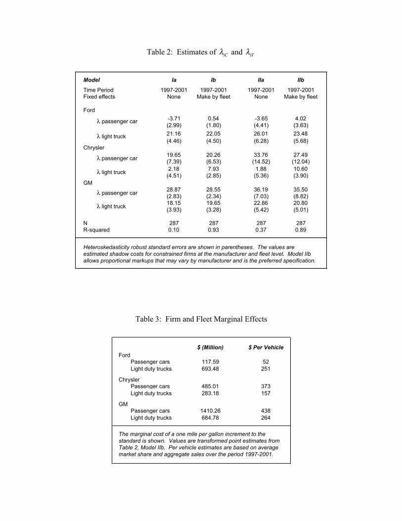
Table 2: Estimates of λiC and λiT

Table 3: Firm and Fleet Marginal Effects

Model Ia Ib IIa IIb

Time Period 1997-2001 1997-2001 1997-2001 1997-2001Fixed effects None Make by fleet None Make by fleet

Ford-3.71 0.54 -3.65 4.02(2.99) (1.80) (4.41) (3.63)21.16 22.05 26.01 23.48(4.46) (4.50) (6.28) (5.68)

Chrysler19.65 20.26 33.76 27.49(7.39) (6.53) (14.52) (12.04)2.18 7.93 1.88 10.60

(4.51) (2.85) (5.36) (3.90)GM

28.87 28.55 36.19 35.50(2.83) (2.34) (7.03) (8.82)18.15 19.65 22.86 20.80(3.93) (3.28) (5.42) (5.01)

N 287 287 287 287R-squared 0.10 0.93 0.37 0.89

Heteroskedasticity robust standard errors are shown in parentheses. The values are estimated shadow costs for constrained firms at the manufacturer and fleet level. Model IIb allows proportional markups that may vary by manufacturer and is the preferred specification.

λ passenger car

λ light truck

λ passenger car

λ light truck

λ passenger car

λ light truck

$ (Million) $ Per VehicleFord

Passenger cars 117.59 52Light duty trucks 693.48 251

ChryslerPassenger cars 485.01 373Light duty trucks 283.18 157

GMPassenger cars 1410.26 438Light duty trucks 684.78 264

The marginal cost of a one mile per gallon increment to the standard is shown. Values are transformed point estimates from Table 2, Model IIb. Per vehicle estimates are based on average market share and aggregate sales over the period 1997-2001.

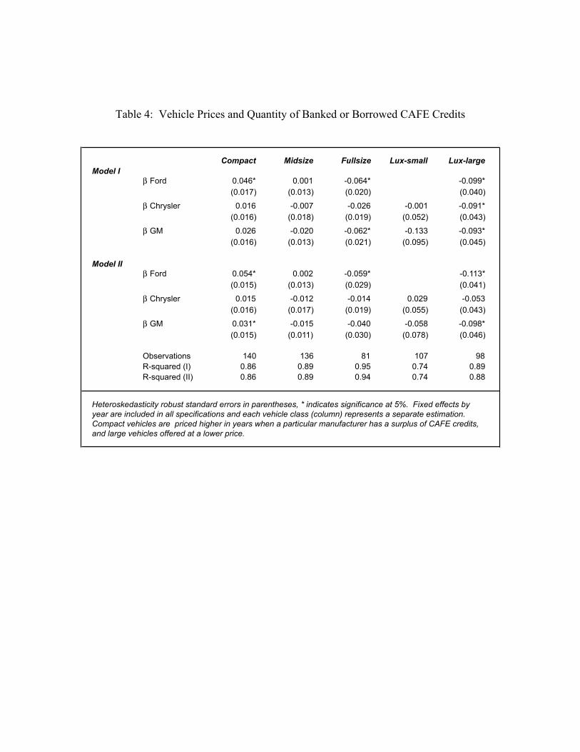
Table 4: Vehicle Prices and Quantity of Banked or Borrowed CAFE Credits

Compact Midsize Fullsize Lux-small Lux-largeModel I

β Ford 0.046* 0.001 -0.064* -0.099*(0.017) (0.013) (0.020) (0.040)

β Chrysler 0.016 -0.007 -0.026 -0.001 -0.091*(0.016) (0.018) (0.019) (0.052) (0.043)

β GM 0.026 -0.020 -0.062* -0.133 -0.093*(0.016) (0.013) (0.021) (0.095) (0.045)

Model IIβ Ford 0.054* 0.002 -0.059* -0.113*

(0.015) (0.013) (0.029) (0.041)

β Chrysler 0.015 -0.012 -0.014 0.029 -0.053(0.016) (0.017) (0.019) (0.055) (0.043)

β GM 0.031* -0.015 -0.040 -0.058 -0.098*(0.015) (0.011) (0.030) (0.078) (0.046)

Observations 140 136 81 107 98R-squared (I) 0.86 0.89 0.95 0.74 0.89R-squared (II) 0.86 0.89 0.94 0.74 0.88

Heteroskedasticity robust standard errors in parentheses, * indicates significance at 5%. Fixed effects by year are included in all specifications and each vehicle class (column) represents a separate estimation. Compact vehicles are priced higher in years when a particular manufacturer has a surplus of CAFE credits, and large vehicles offered at a lower price.

Table 5: Test of CAFE Credit Model for Unconstrained and Fine-Paying Firms

Compact Midsize Fullsize Lux-small Lux-large

β Honda -0.001 -0.001 0.007* 0.001(0.0010) (0.0006) (0.0024) (0.0007)

β Toyota -0.009 0.016 -0.028 0.030 0.035(0.0116) (0.0194) (0.0164) (0.0539) (0.0272)

β Other Asian 0.005 0.012* 0.008 0.012(0.0029) (0.0041) (0.0075) (0.0128)

β European 0.011* 0.008* 0.003 0.018(0.0037) (0.0037) (0.0165) (0.0131)

Observations 140 136 81 107 98R-squared 0.86 0.9 0.94 0.76 0.87

The details of estimation are as in Table 4, now performed for the unconstrained and fine-paying makes. * indicates significance at 5%. The pricing pattern seen for the three makes constrained by CAFE no longer appears, with point estimates either insignificant or comparatively small in magnitude.

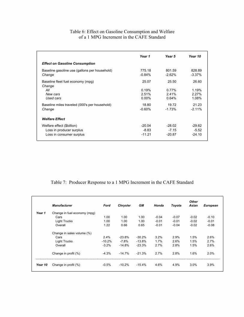
Table 6: Effect on Gasoline Consumption and Welfare of a 1 MPG Increment in the CAFE Standard

Table 7: Producer Response to a 1 MPG Increment in the CAFE Standard

Year 1 Year 5 Year 10

Effect on Gasoline Consumption

Baseline gasoline use (gallons per household) 775.18 801.59 828.89Change -0.84% -2.62% -3.37%

Baseline fleet fuel economy (mpg) 25.07 25.50 26.60Change

All 0.19% 0.77% 1.19%New cars 2.51% 2.41% 2.27%Used cars 0.00% 0.64% 1.08%

Baseline miles traveled (000's per household) 18.80 19.72 21.23Change -0.60% -1.73% -2.11%

Welfare Effect

Welfare effect ($billion) -20.04 -28.02 -29.62Loss in producer surplus -8.83 -7.15 -5.52Loss in consumer surplus -11.21 -20.87 -24.10

Manufacturer Ford Chrysler GM Honda ToyotaOther Asian European

Year 1 Change in fuel economy (mpg)Cars 1.00 1.00 1.00 -0.04 -0.07 -0.02 -0.10Light Trucks 1.00 1.00 1.00 -0.01 -0.01 -0.02 -0.01Overall 1.22 0.66 0.65 -0.01 -0.04 -0.02 -0.08

Change in sales volume (%)Cars 2.4% -23.8% -30.2% 3.2% 2.9% 1.5% 2.6%Light Trucks -10.2% -7.8% -13.8% 1.7% 2.6% 1.5% 2.7%Overall -3.2% -14.8% -23.3% 2.7% 2.8% 1.5% 2.6%

Change in profit (%) -4.3% -14.7% -21.3% 2.7% 2.8% 1.6% 2.0%

Year 10 Change in profit (%) -0.5% -10.2% -15.4% 4.6% 4.9% 3.0% 3.9%

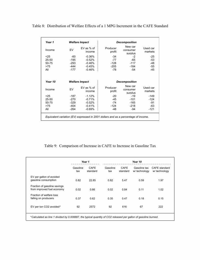
Table 8: Distribution of Welfare Effects of a 1 MPG Increment in the CAFE Standard

Table 9: Comparison of Increase in CAFE to Increase in Gasoline Tax

Year 1 Welfare Impact Decomposition

Income EV EV as % of income

Producer profit

New car consumer

surplus

Used car markets

<25 -60 -0.36% -34 -2 -2525-50 -195 -0.52% -77 -65 -5350-75 -293 -0.46% -128 -117 -48>75 -444 -0.45% -205 -184 -55All -177 -0.46% -78 -54 -45

Year 10 Welfare Impact Decomposition

Income EV EV as % of income

Producer profit

New car consumer

surplus

Used car markets

<25 -187 -1.12% -20 -19 -14925-50 -270 -0.71% -45 -101 -12450-75 -329 -0.52% -74 -165 -91>75 -404 -0.41% -124 -218 -63All -264 -0.69% -48 -94 -121

Equivalent variation (EV) expressed in 2001 dollars and as a percentage of income.

Year 1 Year 10

Gasoline tax

CAFE standard

Gasoline tax

CAFE standard

Gasoline tax w/ technology

CAFE standard w/ technology

EV per gallon of avoided gasoline consumption 0.82 22.85 0.82 5.47 0.59 1.97

Fraction of gasoline savings from improved fuel economy 0.02 0.66 0.02 0.84 0.11 1.02

Fraction of welfare loss falling on producers 0.37 0.62 0.35 0.47 0.18 0.15

EV per ton CO2 avoideda 92 2572 92 616 67 222

aCalculated as line 1 divided by 0.008887, the typical quantity of CO2 released per gallon of gasoline burned.

Table 10: Contribution of Mix-Shifting and Technological Improvements: The Influence of a Footprint Standard

Gasoline tax w/ technology

CAFE standard w/ technology

CAFE standard only technology

Primary incentives for abatement VMT reduction Mix-shifting Technology

XXX

XX

X

EV per gallon of avoided gasoline consumption 0.59 1.97 2.14

Fraction of gasoline savings from improved fuel economy 0.11 1.02 1.01

Fraction of fuel economy improvement from technology 0.90 0.88 1.00

EV per ton CO2 avoided 67 222 241

The three policies shown provide succesively fewer incentives for abatement, with the final "only technology" case coming closest to the current footprint-based standard. The footprint-based standard rewards technology changes, but provides much less incentive to mix-shift to smaller vehicles since the standard itself is raised as a firm's fleet gets smaller.

Table 11: Sensitivity Analysis

Cost per gallon gasoline saved Firm profit impacts in year 1

Gasoline tax w/ technology

CAFE standard w/ technology

Constrained firms

Unconstrained firms

Central case 0.59 1.97 -0.36% 0.25% 1.63

High VMT and low car price elasticitiesa 0.34 3.38 0.07% 0.19% 1.53

Low VMT and high car price elasticitiesa 0.70 1.56 -0.61% 0.35% 1.75

Very low VMT and high car price elasticitiesa 0.79 1.40 -0.73% 0.42% 1.82

High shadow costb 0.59 2.31 -0.59% 0.33% 1.63

Low shadow costb 0.59 1.61 -0.10% 0.17% 1.68

Unit scrap elasticityc 0.61 1.71 -0.32% 0.28% 1.87

Ratio of EV: lowest to highest income quartile

aThe high case is a doubling of λh for each household, low reduces it by half, and very low reduces it to one quarter of the originally estimated value. VMT elasticities rise and fall in proportion to λ while car price elasticities for each case are moved in the opposite direction to maintain the predicted level of VMT for the household.bThe high and low shadow cost cases are constructed by adding or subtracting one standard error (as reported in Table 2) to the baseline value of each constrained firm's shadow cost.cHere the elasticity of vehicle scrap is set to -1 (the central case value is -3).

Figure 1: Toyota, Ford, and BMW: Fleet Fuel Economies

Source: NHTSA CAFE compliance records, 1990-2001.

18

20

22

24

26

28

30

32

34

36

1983 1988 1993 1998 2003

Mile

s pe

r gal

lon

(har

mon

ic m

ean)

Toyota

Ford

BMW

CAFE Standard

Figure 2: Fleet Fuel Economies by Firm Type

Source: NHTSA CAFE compliance records, 1990-2001.

18

20

22

24

26

28

30

32

34

36

1983 1988 1993 1998 2003

Mile

s pe

r gal

lon

(har

mon

ic m

ean)

Constrained Firms

GM Ford Chrysler CAFE Standard

18

20

22

24

26

28

30

32

34

36

1983 1988 1993 1998 2003

Mile

s pe

r gal

lon

(har

mon

ic m

ean)

Unconstrained Firms

Toyota Honda Nissan VW Hyundai CAFE Standard

18

20

22

24

26

28

30

32

34

36

1983 1988 1993 1998 2003

Mile

s pe

r gal

lon

(har

mon

ic m

ean)

Violating Firms

BMW Mercedes Porsche CAFE Standard

Appendix-1

Appendix A: Alternative Specifications and Tests

This appendix extends the econometric model of Section 4 to consider different

forms, fixed effects, and conduct a “placebo” type test on unconstrained firms.

Year fixed effects

My estimation of the shadow costs using a pooled sample rests on the assumption

of relatively stable demand conditions over the period 1997–2001. The second column of

Table A1 shows that the estimates of λ are nearly unchanged when including fixed

effects by year. The estimated coefficients on year are also relevant as they signal

changes in average markups over time: None of the coefficients are significantly

different from zero or one another and their magnitudes are all less than 0.05 in absolute

value.1 This lends some support to the assertion that average markups, and by association

demand conditions, were stable over the years considered.

Structure of fixed effects

The ratio of markups, γ i , is the focus of the literature and also the parameter I

allow to vary by make and fleet in the central case. Column 3 of Table A1 considers the

alternative, where α i is instead allowed to vary and γ is estimated as a scalar. The

coefficients of interest are slightly reduced in magnitude, although all that are significant

in the central specification remain so.

Placebo test

An instructive placebo test is to imagine that the other 4 manufacturers (Honda,

Toyota, Other Asian, and European) are in fact constrained by CAFE around their

1 Change in γ i by model year:

Year 1997 1998 1999 2000 2001 Coefficient omitted -0.002 -0.001 -0.029 -0.042 (SE) (0.024) (0.026) (0.025) (0.026)

Appendix-2

average fuel economy. This allows the construction of the LiC and LiT variables, and

estimation together with the constrained domestic firms. The results appear in column 4

of Table A1. While the coefficients are more often positive than negative none is

significant at the 5% level. The coefficient on European cars is positive and has the

largest t-statistic (1.63), perhaps picking up the effects of the CAFE fines that alter the

pricing of European imports. Note that these vehicles tend to have high base prices and

are part of an aggregate that includes complying companies, so we shouldn’t expect the

difference in markups to be very large. Appendix B: Dynamics of Banking and Borrowing in U.S. CAFE Regulation

This appendix provides an outline of the dynamic decisions made by firms in the

context of CAFE banking and borrowing. Banking and borrowing rules

Under the rules established for the CAFE program, a set of certified fleet fuel

economies is produced for each firm on an annual basis. Deviations from the standard

are first used to offset the firm’s stock of credits or debts, beginning with the oldest.

When no existing credits or debts remain, deviations from the standard are “banked” for

three years into the future. If a firm has debts owed from three years in the past and has

failed to repay them, the firm is found to be in violation and a fine is assessed in the

amount of $50 per vehicle per mile per gallon. Notice that no violation occurs and no

penalties are assessed if the firm repays its debts within three years.

The following example illustrates the accounting method used: the “deviation” in

year t, Yt, takes a positive value if the firm has a fleet fuel economy above the standard,

and a negative value if it is below. The values for δ take a positive value if the firm has

credits that it may use to offset a negative deviation, and a negative value if it has debts it

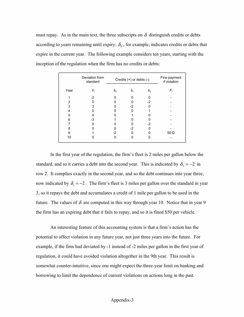
Appendix-3

must repay. As in the main text, the three subscripts on δ distinguish credits or debts

according to years remaining until expiry: δ0 , for example, indicates credits or debts that

expire in the current year. The following example considers ten years, starting with the

inception of the regulation when the firm has no credits or debts:

Deviation from standard Credits (+) or debts (-) Fine payment

if violation

Year Yt δ0 δ1 δ2 Ft

1 -2 0 0 0 -2 0 0 0 -2 -3 3 0 -2 0 -4 0 0 0 1 -5 0 0 1 0 -6 -3 1 0 0 -7 0 0 0 -2 -8 0 0 -2 0 -9 1 -2 0 0 50�Q

10 0 0 0 0 -

In the first year of the regulation, the firm’s fleet is 2 miles per gallon below the

standard, and so it carries a debt into the second year. This is indicated by δ2 = −2 in

row 2. It complies exactly in the second year, and so the debt continues into year three,

now indicated by δ1 = −2 . The firm’s fleet is 3 miles per gallon over the standard in year

3, so it repays the debt and accumulates a credit of 1 mile per gallon to be used in the

future. The values of δ are computed in this way through year 10. Notice that in year 9

the firm has an expiring debt that it fails to repay, and so it is fined $50 per vehicle.

An interesting feature of this accounting system is that a firm’s action has the

potential to affect violation in any future year, not just three years into the future. For

example, if the firm had deviated by -1 instead of -2 miles per gallon in the first year of

regulation, it could have avoided violation altogether in the 9th year. This result is

somewhat counter-intuitive, since one might expect the three-year limit on banking and

borrowing to limit the dependence of current violations on actions long in the past.

Appendix-4

The set of necessary and sufficient conditions for compliance can be written after

defining the evolution of the δ parameters through time. There are four cases that must

be considered. The case of positive δ and negative Y is provided as an example in the

main text; the accounting definitions in the remaining cases are provided below. Notice

that the accounting method means that a firm can not carry both credits and debts at the

same time, so if any δ is positive (negative) all of the others are weakly positive

(negative). For (δ ≥ 0 and Y ≥ 0) or (δ < 0 and Y < 0):

δ0,t+1 = δ1,tδ1,t+1 = δ2,tδ2,t+1 = Yt

For δ < 0 and Y ≥ 0:

δ0,t+1 =δ1,t

δ0,t + δ1,t +Yt0

if Yt ≤ −δ0,t if − δ0,t < Yt < −(δ0,t + δ1,t )otherwise

⎧⎨⎪

⎩⎪

δ1,t+1 =δ2,t

δ0,t + δ1,t + δ2,t +Yt0

if Yt ≤ −(δ0,t + δ1,t ) if − (δ0,t + δ1,t ) < Yt < −(δ0,t + δ1,t + δ2,t )otherwise

⎧⎨⎪

⎩⎪

δ2,t+1 =δ0,t + δ1,t + δ2,t +Yt

0⎧⎨⎩

if Yt > −(δ0,t + δ1,t + δ2,t )otherwise

After computing the evolution of credits and debts as above, the compliance condition

itself can be defined easily. A firm is in compliance with regulation in all years t if and

only if: δ0,t > 0 or Yt > −δ0,t for all t

Appendix-5

The firm’s full maximization problem over time (without discounting) can then be

written as:

max{ pj ,t }

(pj ,t − cj ,t )qj ,t (Pt )j∑

t∑

⎛

⎝⎜⎞

⎠⎟− I(Q) H + FC ,t (Q)

t∑ + FT ,t (Q)

t∑⎛

⎝⎜⎞⎠⎟

⎡

⎣⎢⎢

⎤

⎦⎥⎥

where I(Q) = 0 iff (δ0,t > 0 or Yt > −δ0,t for all t) .

The problem for the unconstrained firm reduces to period-by-period profit

maximization since the right hand term drops out. For constrained firms, however, the

constraint includes multiple discontinuities and the complete history of a firm’s actions

(since I depends on the entire time series of δ0 , δ1 , and δ2 ). In order to simplify the

problem for estimation I define compliance in a single year as Yt ≥ 0. This is a sufficient

condition for compliance in the dynamic model, but abstracts from banking and

borrowing. If demands are certain and stable over time and assuming convex profits with

respect to fleet fuel economy, however, the period-by-period solution to the static

problem coincides with the solution to the full dynamic problem above.

Table A1: Alternative Specifications

Case Central (Model IIb)

Year Fixed Effects

Fixed Effects in α

Unconstrained Makes

Fixed effects (γ) Make by fleet Make by fleet, year - Make by fleet

Fixed effects (α) - - Make by fleet -

Ford4.02 3.75 1.40 3.00

(3.63) (3.87) (2.53) (3.27)23.48 23.56 23.59 22.15(5.68) (5.36) (5.41) (5.33)

Chrysler27.49 27.70 24.98 24.34

(12.04) (11.43) (11.20) (11.28)10.60 10.18 8.22 10.36(3.90) (3.51) (3.05) (3.81)

GM35.50 35.40 31.90 32.59(8.82) (8.87) (6.33) (7.98)20.80 21.11 20.93 19.61(5.01) (5.18) (4.14) (4.70)

Honda2.88

(7.05)-3.14(4.55)

Toyota11.57(7.70)5.75

(3.94)Other asian

-4.44(11.47)

5.65(6.10)

European5.84

(3.57)9.90

(11.01)

N 287 287 287 287R-squared 0.89 0.90 0.89 0.90

Robust standard errors shown in parentheses. The model is column IIb of Table 2, with the indicatedmodifications and additions. Findings from the main text are robust to the alternative forms considered.

λ passenger car

λ light truck

λ passenger car

λ light truck

λ passenger car

λ light truck

"λ" passenger car

"λ" light truck

"λ" passenger car

"λ" light truck

"λ" passenger car

"λ" light truck

"λ" passenger car

"λ" light truck