0

Evaluating the Value-Chain of Freight Trucking: Industry Cluster Analysis and Field of Influence

BY

CARA BADER B.A., University of Iowa, 2004

M.U.P.P., University of Illinois at Chicago, 2011

STUDENT PAPER COMPETITION

Transport Chicago 2011

1

1. Introduction

Freight transportation has a broad effect on the nationʻs economy because it is an essential input in the production process. Investments in transportation infrastructure can produce generative effects for national economic growth. Freight transportation performance affects the economy through the first order benefits directly accrued to carriers and shippers, second order benefits that alter logistics due to improved performance, third order benefits that are derived from a change in the type and quality of goods produced due to new technological advances, and “other effects” including long term job or income growth (HDR|HLB Decision Economics Inc. 2008). Currently, third order benefits are difficult to measure and are often excluded from published statistics. The nationʻs highway system is already congested, and significant public funds will be necessary to build and maintain infrastructure in order to guarantee the effectiveness of freight trucking in the future. A precise accounting of third order benefits is essential to understanding the broad economic benefits of freight infrastructure projects and informed decision making.

This study proposes methods that would better allow decision makers to evaluate the third order benefits of freight infrastructure improvement by centering focus on the industries that will be most prominently affected by a freight trucking project. Although the study does not develop a tool to explicitly quantify these benefits, it examines the location of industries, spatially and economically, that will experience third order benefits and seeks to identify how the benefits are propagated through local economies. The results of this analysis are in furtherance of a future methodology that may quantify third order benefits. The Federal Highway Administration (FHWA) has called for further research into the development of such a tool (HDR|HLB Decision Economics Inc. 2008).

I employ a Wardʻs hierarchical agglomerative cluster analysis using Chebychevʻs distance measure to create a clustered value-chain for the trucking sector in the ten central states of Illinois, Indiana, Iowa, Kansas, Kentucky, Michigan, Minnesota, Missouri, Ohio, and Wisconsin. These ten states represent the planning area of the Mid-America Freight Coalition, and this is the area where comprehensive data was available for this study. This information is used to identify key supplying and purchasing sectors of the truck transportation industry in order to identify the industries that will most likely experience third order benefits. The underlying data referenced are 2007 county level input-output (IO) accounts for the ten central states from the Minnesota IMPLAN Group. Input-output data estimate real-world transactions among all industries in an economy and provide a better picture of industrial interdependence than existing tools provided by the FHWA.

I advance two strategies for isolating the presence of third order benefits in a local economy. First, I use location quotients to identify the specialization of local economies, at the sub-geographic of Economic Areas (defined by the Bureau of Economic Analysis, Appendix A), in the major industries of the trucking value-chain. This information can be used to assist decision makers in placing transportation improvements near areas of trucking industry clusters. Second, I conduct a field of influence analysis on three economic areas in the ten central states region (Chicago, Detroit, and Madison) to examine how technological change is propagated in the economy through interindustry transactions. Field of influence analysis is a relatively new technique that examines the change of technological coefficients in an input-output model.

Industry cluster analysis and field of influence analysis have not yet been applied to regional comparisons of truck transportation. However, the assumptions of the input-output framework that underlies the data and methods pursued in this study provide for a number of limitations on the interpretation of findings. This study points to a number of directions for future

2

research that may be able to overcome these limitations and result in the calibration of an accurate model for quantifying third order benefits.

Section 2 presets a brief review of relevant literature and theoretical background. Section 3 outlines a detailed methodological account with particular emphasis on cluster analysis methods. Section 4 presents the results of the value-chain cluster analysis, mapping of industry specialization, and field of influence analyses. Finally, Section 5 offers some conclusions based on the results presented in the previous section and suggests some directions for future research. While there are still gaps in reaching the goal of measuring third order benefits, as discussed in the conclusion, this study approaches the discussion and measurement of these benefits in a way that has not been previously attempted.

2. Literature Review and Theory

The claim that large scale infrastructure investments cause economic growth has been debated in academic literature, but neither proponents nor critics have developed consistent empirical support (Chandra and Thompson 2000). Attempts to measure the economic impacts of freight policy specifically are the exception rather than the rule. Freight transportation planning is often neglected in long term transportation plans, because of the inherent difficulty in connecting alterations in freight policy to tangible benefits for taxpayers (Seetharaman, Kawamura and Dev Bhatta 2003).

Input-output analysis, pioneered by Wassily Leontief (1939), is one of the most widely applied methods in economics. Miller and Blair (1985) cite the fundamental purpose of the input-output model as to enable analysis of the interdependence of industries in an economy. The heart of the model is a transactions table (also called the interindustry transactions matrix).The table is an NxN matrix based on N industries in the economy. Each row of the table lists the outputs (credits/sales) of each industry separated into recipient industries. Each column lists the inputs (debits/purchases) used by the industry in production separated by source industry. Therefore each row describes the distribution of a producerʼs output throughout the economy and each column describes the inputs required for an industry to produce. In a one period input-output model, each column represents the cost function for the represented industry (Leontief 1939).

A fundamental assumption of the input-output framework is that interindustry purchases, such as from industry i to industry j, are dependent solely on the total output of industry j (Miller and Blair 1985). The value of purchases from industry i to industry j relative to total purchases by industry j is the technical coefficient. This is also called the direct requirements matrix. The Leontief system assumes technical coefficients are unchanging, returns to scale are constant, and sectors use inputs in fixed proportions (Miller and Blair 1985). Represented industries employ a uniform production process and do not alter the process based on scale, supply constraints, or price changes.

The coefficients present in the direct requirements matrix do not reflect the cost of indirect inputs used by industry i to produce the goods sold as inputs to industry j. The values of the additional purchases of indirect inputs, as well as the value of direct inputs are reflected in the total requirements matrix. The total requirements matrix is calculated by subtracting the direct requirements matrix, or A matrix, from an identity matrix, I, and inverting the resulting matrix. Each cell of the total requirements matrix, also referred to as the Leontief inverse matrix, represents the total dollar value of input, direct and indirect, exchanged between industries to produce one dollar worth of output from the industry in question.

Input-output analysis is often used in tandem with impact and multiplier analysis. Impact analysis seeks to identify the impact on a defined economy of a change, or changes, in the final

3

demand for difference sectors based in the economy. This is calculated using total requirement coefficients of an input output model. Input-output multipliers are summary measures derived from the Leontief inverse matrix that indicate the total economic effect of one dollar spent in an industry.

The basic model is a static model; the data and technology implied represent one period. Therefore the model does not represent technological change because production functions are fixed. The input-output framework is constructed from a demand side perspective that assumes products will come through the economic structure to meet demand; there are no supply shortages or substitutions. The model assumes that industries produce homogenous outputs, and it does not account for industries that produce auxiliary goods under another sector. Finally, the model itself is only concerned with backward linkages, or what goes into making the good. It cannot evaluate how the demand for goods that accompany a product will change because of higher demands.

Industry cluster analysis has been defined as “the systematic identification and documentation of key groups of interdependent businesses in an economy”(Feser and Luger 2003). Industry cluster principles are often used in tandem with traditional development schemes to improve the effectiveness of implementation of existing policy. All cluster policies are focused on the related goals of resource targeting and resource leveraging. Industry cluster analysis is used by policymakers to identify targets for scarce development resources in order to leverage these resources through synergies, positive externalities, and increasing returns believed to exist within the clusters (Feser 1998).

The goal of industry cluster analysis is to allow policy officials to gain unique insight into the basic features of their regional economy by focusing on industry linkages and interdependence among firms (Bergman and Feser 1999). Input-output accounts are one of the few measures of interfirm relationships available to analysts at wide geographic scale (Feser 1998). Additionally, the focus on buyer-supplier relationships that input-output matrices provides allows for analysis that documents trade flows among many, some unexpected, industries (Roelandt, et al. 1999).

The input-output framework also offers the ability to study innovations in groups of industries. Perroux suggests that innovations are not only clustered in time, as theorized by Schumpeter (1934), but also in economic space (Perroux 1998). Technological advances establish paths for innovation to travel throughout economic space through the adoption of learning processes in economically linked industries. Understanding the other industries present in an extended value chain can aid firms in making location decisions and can assist local economic developers in targeting efforts (Peters 2001; Bergman and Feser 1999; Feser and Bergman 2000; Feser 2005).

The underlying logic for building specialization in these industries lies in the economic base model (Krikelas 1992), evolutionary regional development theory (Thompson 1965), and new growth theory (Griliches 1992). All of these models in one form or another advocate concentration in specialized industries. Evolutionary regional development and new growth theories also seek to capitalized on the increasing returns to scale that exist in some clusters.

There is a general consensus that linkages between sectors in an economy are important for economic growth as first theorized by Perroux; however, the process by which these key linkages are identified is still contentious(Sonis, Guilhoto, et al. 1995). The objective of linkage analysis is to quantify the impacts of a change in one sector on other related sectors (Kawamura, Sriraj and Lindquist 2009).

The fields of influence technique was developed to analyze more precisely the impacts of a change in one sector on the rest of the economy (Sonis, Guilhoto, et al. 1995). The concept of a field of influence is based on the idea that a change in technical requirement based in one

4

cell will alter the total requirements coefficients (Leontief inverse matrix) of many cells. The interindustry purchasing patterns of all industries that interact with the two industries affected by the initial change will be altered. Therefore, the Leontief inverse matrix after the change in one cell is equal to the original matrix plus a matrix representing the field of influence (all of the changes due to the initial change)(Sonis and Hewings 2009).

The first order field of influence describes the changes that occur due to only one element (cell) of the matrix. A second order field of influence examines the synergistic interactions of two simultaneous changes in the matrix. Fields of influence of k orders can be analyzed using a recurring combination of the mathematical formulae for the first and second order (Sonis, Guilhoto, et al. 1995). Additionally, Sonis and Hewings (1994) outline how the fields of influence concept could be applied to address changes in a complete row, column, or the whole matrix.

3. Methods 3.1. Isolate Value-Chain Clusters Value chain clusters for the freight truck transportation industry are calculated based on industry to industry transactions data in 2007. The sample area is the 10 central states of Illinois, Indiana, Iowa, Kansas, Kentucky, Michigan, Minnesota, Missouri, Ohio and Wisconsin. The region was chosen for two reasons: data availability and the regional variability of the relationship of freight to the rest of the economy. This suggests that although the common reference economy for an input-output study is the nation as a whole, it is more appropriate to compare economic areas in the central region to an aggregate measure of the central region rather than the nation as a whole.

The variable to be clustered is the total dollar value of the transaction between two industries. Backward linkage clusters are calculated based on the column transactions of IMPLAN Industry Code 335, transport by truck, in an input-output model of the 10 central states. Column transactions represent the dollar value of the truck transportation industryʼs intermediate input purchases from every other industry represented in the economy. Forward linkage clusters are calculated based on the row transactions of industry 335, transport by truck, in an input-output model of the 10 central sttes. Row transactions represent the dollar value of truck transportation sold to all other industries in the economy. In order to ease interpretation and validation of the cluster solution the transaction values were standardized. Transaction values were standardized to range from zero to one by transforming them into trading linkage ratios using same method as Feser, Renski, and Koo (2008). This study employs Wardʼs hierarchical agglomerative clustering algorithm in SPSS using Chebychevʼs distance measure. Hierarchical agglomerative methods are the most commonly used clustering methods(Aldenderfer and Blashfield 1984). The hierarchical agglomerative method begins under the assumption that every case is an independent cluster. An N N similarity matrix is constructed that describes the similarity (or difference) between each case and every other case to be considered for clustering. Distance measures are technically measures of dissimilarity; two identical points are a distance of zero apart. Distance measures are a similarity measure in reverse scale. The values of distance measures have no absolute meaning. This study employs Chebychevʼs distance measure. This distance measure is appropriate when using centroid, median or Wardʼs method of clustering. The formula representation of Chebychevʼs distance is featured in Appendix B. The distance between two cases is the maximum absolute distance between all of the values of

5

the clustering variables. In this case, transactions are the only variable used to determine clusters, so the distance is the absolute difference between two cases. The hierarchical clustering method proceeds by finding the two most similar cases in the similarity matrix and merging them to form a cluster. The method continues for N-1 steps until all cases are merged into one large cluster. Different clustering methods vary by the linkage rules used to compare clusters to each other as the process moves along. The hierarchical method produces nonoverlapping clusters, meaning each case is a member of only one cluster. As the process proceeds each cluster can be subsumed as a member of a larger cluster at a higher level of similarity.

Wardʼs linkage method uses an analysis of variance approach to analyze the distance between two considered cases. This method is designed to find the minimum variance within clusters; it works by joining groups or cases that result in a minimum increase in the within group sum of squares. The formulation of the within-group sum of squares in Wardʼs method is outlined in Appendix B. This method tends to create clusters of relatively equal sizes and shaped by hyperspheres; it has been widely used in the social sciences (Aldenderfer and Blashfield 1984). Validating a cluster solution can be conceptually difficult. There is a lack of an agreed upon null hypothesis for statistically evaluating a cluster solution. The process of performing a cluster analysis creates the structure within the data, it is therefore impossible to then evaluate the case that there is no inherent structure in the data. However, given this limitation, there are a number of techniques used to determine the appropriate number of clusters formed in the analysis. This paper examines the loss of information, or fusion coefficients, at the end stages of the clustering process and performs an ANOVA test on the clustering solution. Although both of these techniques introduce some level of subjectivity, they are widely used.

In order to determine the number of clusters that can be appropriately assumed to exist within the data, the analyst needs to determine the stage of the clustering process at which a critical loss of information occurs. A loss of information is interpreted as the merger of two highly dissimilar clusters; merging the two dissimilar clusters creates a loss of information that can be gleaned from viewing the clusters as separate groupings of data. One procedure for determining the cluster solution is to examine the fusion coefficients in a list and look for a significant “jump” in the value (Aldenderfer and Blashfield 1984). This process can be aided by listing the change in the fusion coefficient, or loss of information, next to the fusion coefficient. The number of clusters prior to the jump is the most likely solution. Peters (2001) puts forth an additional method for validating the cluster solution. He conducts an analysis of variance using the number of cases in each cluster, the mean non-standardized value of cases within the cluster, and the standard deviation of non-standardized values within the cluster. He uses this information to statistically demonstrate that the input cases for each cluster are significantly different. Although this is a statistically valid way of proving the cluster solution, it is almost guaranteed since the clustering result will group industries by value of purchase. 3.2. Economic Area Specializations in Value-Chain Clusters

Individual economic areas (EA) are compared using location quotients in order to evaluate the economic areasʼ specialization in industries that are significant in the value chain for freight truck transportation. Location quotients measure concentration of a given industry, or group of industries, in the study economy compared to a reference economy. The same reference economy used to calculate the clusters, the 10 central states, is used as the reference economy to calculate location quotients. The formula for a location quotient is as follows:

6

The numerator is the share of total output in the economic area that comes from the industries cluster, and the denominator is the share of total output in the 10 states region that comes from the industries within the cluster. The location quotients for each EA and each cluster of industries are joined to spatial depiction of the EA in ArcGIS. This information is used to create a map of each EAʼs specialization level displayed by category for each cluster group. The specializations are symbolized in grayscale. 3.3. Field of Influence

The field of influence analysis is performed on input-output models of Chicago-Naperville-Michigan City, IL-IN-WI (EA 32), Detroit-Warren-Flint, MI (EA47), and Madison-Baraboo, WI (EA101). The data for these models were derived from input-output models created in IMPLAN. The interindustry transactions, total output, value added and final demand values were taken from the Industry-by-Industry Transactions report and the Industry Output Outlay Summary provided to me by the University of Toledo.

The analysis is performed in PyIO, an input-output analysis tool developed and released by the Regional Economic Applications Laboratory (REAL) at the University of Illinois Champaign-Urbana. In order to be loaded into PyIO, the data must be organized into an ASCII text file. An example of the proper formatting is included in the PyIO Manual (Nazara, et al. 2003). I loaded the data into PyIO in the most disaggregated form available. Each industry in the economy was listed individually. In order to ease the viewing of the results, I used PyIO to aggregate the input-output models into 21 sectors. Also, forward linkage clusters are only included for the purpose of this field of influence analysis because there is overlap among industries in forward and backward linkage clusters; therefore, the backward linkage clusters cannot be aggregated because the same industry would have to be included in multiple clusters, which violates the input-output model. Finally, truck transportation is included as its own sector, apart from the clusters, in order to isolate the effect of a change in only trucking technology.

The field of influence is performed on the aggregated input-output table in PyIO. This study evaluates a change in intraindustry technology between the truck transportation row and truck transportation column, cell (10, 10). PyIO calculates the first order field of influence only. The technical formulation of the first order field of influence is reproduced in Halpern-Givens (2010). The result of the field of influence analysis is a matrix that depicts the incremental change in the Leontief inverse matrix due to a scalar change in the cell specified. The new Leontief inverse coefficient can be calculated by adding the incremental change of the field of influence output to the original Leontief inverse coefficient. 4. Results The value chain clusters for truck transportation are groups of industries that purchase freight truck transportation and industries that the truck transportation industry purchases goods from. These industries are clustered based on the total dollar value of their purchases. Industries with similar values of purchase are grouped together in a cluster according the Wardʼs hierarchical agglomerative clustering method using Chebychevʼs distance measure as outlined in the

7

methods section. Backward linkage clusters are comprised of groups of industries that the truck transportation industry purchases goods from (inputs to trucking) in statistically similar amounts, as determined by the clustering method. Forward linkage clusters are comprised of groups of industries that purchase truck transportation (destinations of trucking output) in statistically similar amounts. 4.1.1. Backward Linkage Clusters

The results of the clustering method suggest the presence of three distinct clusters. The industries present in each cluster and the total dollar value of input purchases by truck transportation are listed in Table I.

The three cluster solution is validated by examination of the fusion coefficients along the agglomeration schedule (Table II) and the ANOVA test (Table III). The table shows a significant jump in the loss of information moving from the three cluster solution to the two cluster solution. This suggests that the three cluster solution is appropriate. The ANOVA results show that the input variable, the value of purchases, is significantly different between the three clusters. Therefore the differences in purchase values that exist between the clusters can be viewed as statistically significant. This allows us to interpret the cluster result as depicting industries that supply the truck transportation industry in significantly different intensities.

Table I. Backward Linkage Industry Clusters

Cluster Industry Code Industry Purchases

1 335 Transport by truck $3,712,680,886 1 115 Petroleum refineries $3,419,000,750 1 427 US Postal Service $3,317,860,229 1 357 Insurance carriers $2,668,872,979 1 339 Couriers and messengers $2,415,738,616 1 382 Employment services $1,948,090,447 2 319 Wholesale trade businesses $1,126,914,277 2 338 Scenic, sightseeing, and support activities for transportation $1,020,802,518 2 384 Office administrative services $935,417,734 2 360 Real estate establishments $906,928,089 2 283 Motor vehicle parts manufacturing $900,130,758 2 381 Management of companies and enterprises $899,705,652 2 333 Transport by rail $841,848,938 2 340 Warehousing and storage $704,773,531 2 388 Services to buildings and dwellings $564,890,467 2 414 Automotive repair and maintenance, except car washes $514,020,147 2 351 Telecommunications $480,365,334 2 354 Monetary authorities, depository credit intermediation acts. $457,186,186 3 --- ALL OTHER INDUSTRIES $4,726,962,833

8

Table II. Backward Linkage Clusters List of Fusion Coefficients

Stage Clusters Fusion Coefficient Loss of Information 415 1 0.949 0.492 414 2 0.457 0.211 413 3 0.246 0.063 412 4 0.183 0.042 411 5 0.141 0.034

Table III. ANOVA Results

ANOVA F = 3431.360 p = 0.000

Cluster N Mean Standard Deviation

1 6 $2,913,707,318 677842520.7 2 12 $779,415,303 227206137.3 3 398 $11,876,791 35425924.57

The first cluster contains industries that can be described as providing primary inputs to

truck transportation. The primary inputs cluster contains industries that supply the greatest dollar value of inputs to truck transportation. Most of these industries would be anticipated to supply a high value of inputs to transport by truck including the industry itself, petroleum refiners, insurance carriers, and employment services. Intraindustry transactions represent the highest total dollar value of transactions in this cluster. This is likely due to subcontracting relationships that characterize many elements of the trucking industry.

The second cluster contains industries that can be described as providing secondary inputs to truck transportation. These industries supply goods in significant amounts, but not as intensely as the primary input suppliers. Significant industries include wholesale trade business, real estate establishments, motor vehicle parts manufacturing, transport by rail, warehousing and storage, and automotive repair and maintenance, telecommunications, and monetary authorities. These industries are not surprising taking into consideration the needs of the trucking industry. Wholesale and warehousing and scenic and sightseeing transportation are the highest value industries in this cluster. Although wholesaling and warehousing represent significant partners with freight, this industry may be artificially inflated by the IMPLAN aggregation scheme. IMPLAN sectors are not aggregated to represent similar levels of detail between general sectors in the economy. In the case of manufacturing, the IMPLAN aggregation scheme goes into great detail in dividing industries based on specialized product orientation, but in the case of wholesale and warehousing, a wide variety of industries with different orientations are grouped into one category. Therefore, the wholesale and warehousing ranks highly because it is a large sector, in terms of categorization, and a large supplier to trucking.

The third cluster contains industries that can be described as providing tertiary inputs to truck transportation. These are the industries that truck transportation purchases inputs from in the least amounts per year. There are 398 industries in this cluster. The truck transportation

9

industry does not zero inputs from many of these industries. The industries with the largest input values in this cluster are management and technical consulting, accounting and bookkeeping, and investigation and security services.

4.1.2 Forward Linkage Clusters

The results of the clustering method suggest four distinct clusters. The industries present in each cluster and the total dollar value of purchases of truck transportation output are listed in Table IV. Many more industries purchase truck transportation in significant amounts than is the case for backward linkages; because of this the clusters suggested are larger and more diverse.

The four cluster solution is validated by examination of the fusion coefficients along the agglomeration schedule (Table V) and the ANOVA results (Table VI) The data values used to determine the clustering method are more similar in the case of forward linkage clusters; every industry purchases some service from truck transportation. This relative decrease in variability makes the distinction between a three cluster and a four cluster solution somewhat more subjective.

In the case of the forward linkage clusters the change in the loss of information is more subtle, but there is a jump that occurs when moving from the four cluster solution to the three cluster solution. This indicates that the four cluster solution is appropriate. A jump is also evident between the three cluster solution and the two cluster solution. The four cluster solution was chosen in order to present more disaggregated information to provide reference for other analysts. Although this introduces some element of bias, in this case the clustering solution is not meant to indicate that there is a structural barrier between the clusters. These clusters are meant to provide analytical categories about the significance of purchases of truck transportation from industries within the economy. An ANOVA F-test on the four cluster solution shows that the differences of the input variable, purchases of truck transportation output, are statistically significant. This suggests that the clusters are significantly different.

The first cluster contains the industries that represent the primary forward linkages of the transport by truck industry. This group purchases the highest amount of freight trucking per year and contains 13 industries. The most significant output recipient is the trucking industry itself. However, agriculture, automobile manufacturing, construction, and food distribution industries are also represented within the cluster. Once again, intraindustry transactions are the highest value because of the subcontracting relationships that characterize the freight industry. Owner-operators sell their services, which is output by a small firm in itself, to other firms in the trucking industry. The other industries in this cluster are not surprising; they represent firms that would likely need trucking to transport products to other firms or retail outlets.

The second cluster contains industries that have secondary forward linkages to truck transportation. These 34 industries purchase significantly more trucking than the industries in the tertiary cluster per year. Additional industries from the sectors represented in the primary cluster are prevalent. However, aircraft manufacturers, paper milling, retail stores, chemical manufacturing, and state and local government enterprises are also represented.

The third cluster contains industries that have tertiary forward linkages to truck transportation. These industries purchase a moderate amount of transportation by truck and there are 160 industries in this cluster. This cluster is much larger and more diverse than the previous two clusters. Other freight transportation industries (air, rail, etc.), chemical and pharmaceutical manufacturing, breweries and distilleries, the U.S. Postal service, metal manufacturing, dairy, and many specialized manufacturing industries are members of this cluster. A full listing of tertiary linkage industries is listed in Appendix C.

10

Table IIII. Forward Linkage Cluster Industries

Cluster Industry Code Industry Purchases

1 335 Transport by truck $3,712,680,886

1 37 Construction of new residential permanent site single- and multi-family structures $1,901,212,509

1 59 Animal (except poultry) slaughtering, rendering, and processing $1,552,918,867 1 283 Motor vehicle parts manufacturing $1,286,830,134 1 170 Iron and steel mills and ferroalloy manufacturing $1,239,966,308 1 277 Light truck and utility vehicle manufacturing $1,128,062,584 1 319 Wholesale trade businesses $975,499,871

1 34 Construction of new nonresidential commercial and health care structures $825,791,336

1 161 Ready-mix concrete manufacturing $822,488,974 1 413 Food services and drinking places $745,577,642 1 45 Soybean and other oilseed processing $677,834,133 1 36 Construction of other new nonresidential structures $596,675,523 1 276 Automobile manufacturing $558,914,051 2 39 Maintenance and repair construction of nonresidential structures $469,566,351 2 54 Fruit and vegetable canning, pickling, and drying $436,161,259 2 105 Paper mills $433,774,338 2 286 Other aircraft parts and auxiliary equipment manufacturing $430,839,221 2 56 Cheese manufacturing $409,261,685 2 38 Construction of other new residential structures $402,629,238 2 397 Private hospitals $393,164,029 2 107 Paperboard container manufacturing $375,873,841 2 381 Management of companies and enterprises $370,588,560 2 44 Wet corn milling $353,744,201 2 130 Fertilizer manufacturing $353,440,074 2 225 Other engine equipment manufacturing $351,649,269 2 361 Imputed rental activity for owner-occupied dwellings $317,813,107 2 126 Other basic organic chemical manufacturing $314,064,885 2 320 Retail Stores - Motor vehicle and parts $295,167,362 2 2 Grain farming $291,654,160 2 55 Fluid milk and butter manufacturing $276,550,336 2 99 Wood windows and doors and millwork manufacturing $275,533,698 2 127 Plastics material and resin manufacturing $272,233,853 2 394 Offices of physicians, dentists, and other health practitioners $269,537,853 2 329 Retail Stores - General merchandise $253,005,664

Forward Linkage Cluster Industries (continued)

11

Cluster Industry Code Industry Purchases

2 42 Other animal food manufacturing $250,789,693 2 164 Lime and gypsum product manufacturing $243,262,065 2 149 Other plastics product manufacturing $243,145,706

2 216 Air conditioning, refrigeration, and warm air heating equipment manufacturing $237,840,257

2 11 Cattle ranching and farming $235,526,460 2 70 Soft drink and ice manufacturing $235,044,940 2 171 Steel product manufacturing from purchased steel $232,888,271 2 414 Automotive repair and maintenance, except car washes $232,063,654 2 324 Retail Stores - Food and beverage $218,019,415 2 31 Electric power generation, transmission, and distribution $212,698,769 2 136 Paint and coating manufacturing $205,551,872 2 432 Other state and local government enterprises $199,597,334 2 41 Dog and cat food manufacturing $198,091,166 3 See Appendix D 4 ALL OTHER INDUSTRIES

Table V. Forward Linkage Clusters List of Fusion Coefficients

Stage Number of Clusters Fusion Coefficient Loss of Information

430 1 .711 0.255 429 2 .456 0.113 428 3 .343 0.083 427 4 .260 0.054 426 5 .206 0.040 425 6 .166 0.030

Table VI. ANOVA Results Forward Linkage Clusters

ANOVA F = 312.769 p = 0.000

Cluster N Mean Standard Deviation 1 13 $1,232,650,217 842484655.4 2 34 $302,669,782 80149855.81 3 160 $79,738,302 38610771.56 4 224 $15,090,721 10178309.53

12

The fourth cluster contains 224 industries that have quaternary forward linkages to trucking. Industries in this cluster purchase the smallest amount of truck transportation per year. This is the largest cluster, and it contains all other industries not previously listed. These industries use truck transportation as an input with the least amount relative to the trucking industryʼs total sales compared to industries in the other three clusters.

It is important to note that these clusters describe the industries that the trucking industry is most dependent on in terms of supplying inputs and demanding trucking services. The variable used to create the clusters relates total transactions between trucking and an industry, relative to the total purchases (or sales) of the trucking industry. Therefore, inclusion of these industries in the clusters does not necessarily indicate that trucking is a critical component of that industryʼs inputs requirements or sales. This clustering analysis revealed the industries that are highly linked to trucking in terms of truckingʼs needs and sales. Including an additional variable into the clustering method that measures the significance of a transaction between trucking an another industry compared to that industries total input spending or total sales would also indicate that industryʼs relative dependence on trucking as an input or a demand source. This is discussed more in the conclusion.

4.2. Specializations of Economic Areas

The economic structure of each economic area (EA) in the 10 central states region

varies based on the industries present in each economy. Economic structure also varies because of concentration in certain economic activities or industries within an EA compared other areas. Location quotients are calculated in order to evaluate how different EAs within the 10 states region are more or less specialized in industries that are significantly involved in the value chain for truck transportation. The industries in the primary and secondary forward linkage clusters are aggregated into one sector representing the entire cluster. This enables evaluation of an economic areaʼs specialization in the most important industries along the value chain as a whole. In order to remain concise presentation of the backward linkage cluster specializations and tertiary forward linkage clusters have been omitted from this paper, but can be calculated in the same manner as presented in the methods.

Table VIII lists the location quotient of each economic area in each of the primary and secondary linkage clusters. For the purpose of this analysis, these location quotients (LQ) are divided into indices of specialization as follows:

High Specialization: LQ ≥ 1.25 Above Average Specialization: 1.05 ≤ LQ < 1.25 Average Specialization: 0.95 ≤ LQ < 1.05 Below Average Specialization: 0.75 ≤ LQ < 0.95 Low Specialization: LQ < 0.75

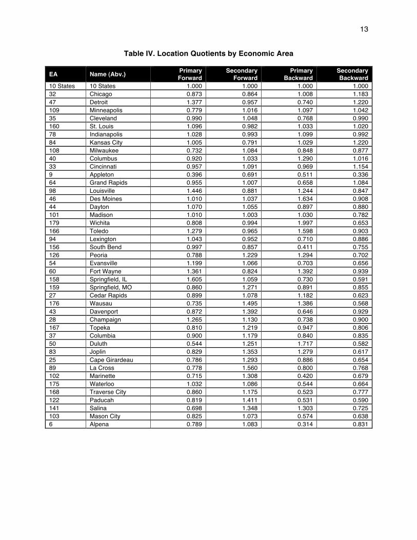
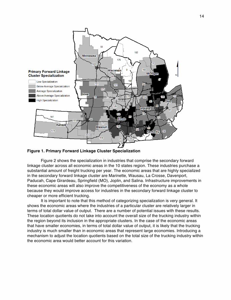
Figure 1 shows specialization in industries in the primary forward linkage cluster across all of the economic areas in the 10 states. These are the industries are the largest purchasers of truck transportation output. The economic areas that highly specialized in this group of industries are Detroit, Toledo, Fort Wayne, Louisville, Champaign, and Springfield (IL). An infrastructure project has the potential to make truck transportation cheaper or more efficient, especially for industries in the primary forward linkage cluster. Economic areas that are specialized in these industries will become more competitive as a result of infrastructure investments because of the savings to important industries.

13

Table IV. Location Quotients by Economic Area

EA Name (Abv.) Primary Forward

Secondary Forward

Primary Backward

Secondary Backward

10 States 10 States 1.000 1.000 1.000 1.000 32 Chicago 0.873 0.864 1.008 1.183 47 Detroit 1.377 0.957 0.740 1.220 109 Minneapolis 0.779 1.016 1.097 1.042 35 Cleveland 0.990 1.048 0.768 0.990 160 St. Louis 1.096 0.982 1.033 1.020 78 Indianapolis 1.028 0.993 1.099 0.992 84 Kansas City 1.005 0.791 1.029 1.220 108 Milwaukee 0.732 1.084 0.848 0.877 40 Columbus 0.920 1.033 1.290 1.016 33 Cincinnati 0.957 1.091 0.969 1.154 9 Appleton 0.396 0.691 0.511 0.336 64 Grand Rapids 0.955 1.007 0.658 1.084 98 Louisville 1.446 0.881 1.244 0.847 46 Des Moines 1.010 1.037 1.634 0.908 44 Dayton 1.070 1.055 0.897 0.880 101 Madison 1.010 1.003 1.030 0.782 179 Wichita 0.808 0.994 1.997 0.653 166 Toledo 1.279 0.965 1.598 0.903 94 Lexington 1.043 0.952 0.710 0.886 156 South Bend 0.997 0.857 0.411 0.755 126 Peoria 0.788 1.229 1.294 0.702 54 Evansville 1.199 1.066 0.703 0.656 60 Fort Wayne 1.361 0.824 1.392 0.939 158 Springfield, IL 1.605 1.059 0.730 0.591 159 Springfield, MO 0.860 1.271 0.891 0.855 27 Cedar Rapids 0.899 1.078 1.182 0.623 176 Wausau 0.735 1.495 1.386 0.568 43 Davenport 0.872 1.392 0.646 0.929 28 Champaign 1.265 1.130 0.738 0.900 167 Topeka 0.810 1.219 0.947 0.806 37 Columbia 0.900 1.179 0.840 0.835 50 Duluth 0.544 1.251 1.717 0.582 83 Joplin 0.829 1.353 1.279 0.617 25 Cape Girardeau 0.786 1.293 0.886 0.654 89 La Cross 0.778 1.560 0.800 0.768 102 Marinette 0.715 1.308 0.420 0.679 175 Waterloo 1.032 1.086 0.544 0.664 168 Traverse City 0.860 1.175 0.523 0.777 122 Paducah 0.819 1.411 0.531 0.590 141 Salina 0.698 1.348 1.303 0.725 103 Mason City 0.825 1.073 0.574 0.638 6 Alpena 0.789 1.083 0.314 0.831

14

Figure 1. Primary Forward Linkage Cluster Specialization

Figure 2 shows the specialization in industries that comprise the secondary forward linkage cluster across all economic areas in the 10 states region. These industries purchase a substantial amount of freight trucking per year. The economic areas that are highly specialized in the secondary forward linkage cluster are Marinette, Wausau, La Crosse, Davenport, Paducah, Cape Girardeau, Springfield (MO), Joplin, and Salina. Infrastructure improvements in these economic areas will also improve the competitiveness of the economy as a whole because they would improve access for industries in the secondary forward linkage cluster to cheaper or more efficient trucking.

It is important to note that this method of categorizing specialization is very general. It shows the economic areas where the industries of a particular cluster are relatively larger in terms of total dollar value of output. There are a number of potential issues with these results. These location quotients do not take into account the overall size of the trucking industry within the region beyond its inclusion in the appropriate clusters. In the case of the economic areas that have smaller economies, in terms of total dollar value of output, it is likely that the trucking industry is much smaller than in economic areas that represent large economies. Introducing a mechanism to adjust the location quotients based on the total size of the trucking industry within the economic area would better account for this variation.

15

Figure 2. Secondary Forward Linkage Cluster Specialization

4.3. Field of Influence Analysis

The field of influence technique is designed to track the diffusion of coefficient change in the direct requirements matrix through the Leontief inverse matrix. The technique has been theorized to address a process or product innovation in one sector that affects all other sectors. This would be represented by a change in an entire column or row of the technical requirements matrix. However, PyIO is currently capable only of modeling a change in one cell of the technical requirements matrix. This is akin to the technology change between two sectors of the input-output model specifically, rather than the entire economy.

This thesis has shown that certain industries have stronger links, on the basis of the total dollar value of purchases, to the truck transportation industries than others. These industries are included in the primary and secondary forward and backward linkage clusters. Furthermore, individual economies within a region differ in economic structure. Differences in economic structure were represented graphically in the previous section, but are also evident in input-output models. This section will evaluate how coefficient change in the truck transportation industry spreads throughout the Leontief inverse matrix in three different economic areas: Chicago-Naperville-Michigan City, IL-IN-WI (EA32), Detroit-Warren-Flint, MI (EA47), and Madison-Baraboo, WI (EA101).

It is expected that the field of influence results will differ in the three regions because of the differences in economic structure. Also, it is expected that the Leontief inverse changes will be largest in the primary and secondary linkage clusters because they represent the strongest ties to the freight trucking industry. However, because some industries are present in both forward linkage clusters and backward linkage clusters, only the backward linkage clusters are represented in the input-output models. The truck transportation industry has been left out of the

16

primary backward linkage cluster in order to isolate its individual effect on the rest of the economy.

The field of influence analysis is performed for a change in technical coefficient in the truck transportation column and the truck transportation row. This cell describes the intraindustry transactions between trucking such as fleet organization purchases and subcontracting relationships. This cell was chosen because the industry interacts with itself in the largest dollar value, and this is the industryʼs most significant link. Also, the spread of technological innovation that occurs as a result of an improvement in transportation infrastructure will begin with a change in efficiency of the freight trucking industry. The field of influence analysis assumes an initial scalar coefficient change, so the cell chosen will show a change greater than unit change. An example of the technological change that is represented by altering this cell would be a fleet composition change that occurs within trucking firms as a result of an infrastructure improvement.

Appendix D shows the results of a field of influence analysis performed on a model of the Chicago economic area. The cells that show an above average change are shaded in gray, and the top ten cell changes are outlined in black. The largest change occurs in the trucking-to-trucking cell, where the field of influence was performed (1.1006). This makes sense as the largest change because the value of “1” is assumed as a part of the field of influence analysis. The largest residual change is actually shown in the cell relating the trucking industryʼs purchase of general manufacturing goods (not a part of the linkage clusters). This confirms Halpern-Givensʼ (2010) findings of strong linkages between trucking and manufacturing. All of the largest cell changes are in the column of trucking, indicating that coefficient change is spread more strongly through backward linkages. Also, the changes in Transportation & Warehousing, Finance & Insurance, and Administrative Services are all larger than the changes experienced to either of the backward linkage clusters. Although the coefficients depicting the cluster industriesʼ purchase of truck transportation does show above average change, it is not in the top ten values. Also, stronger change is experienced in the trucking industryʼs purchase of goods from the secondary backward linkage cluster. That may be because this cluster has more industries.

In order to preserve space, the matrix results for the field of influence analysis for Detroit and Madison are withheld from display here. For Detroit, the above average values fall exclusively in the column and row of the trucking industry. In this case, the largest residual change is within the trucking industry. The top ten values are contained within the same cells as the Chicago region. The magnitude of the changes, however, is smaller in the Detroit model compared to Chicago. Detroit is more specialized than Chicago in the industries of the forward linkage clusters. The region is highly specialized in the primary forward linkage cluster, and the magnitude of this change in the Detroit region (0.093) is larger than Chicago (0.091). However, this difference is very small. Also, Chicago is specialized below average in industries in the secondary forward linkage cluster. The magnitude of coefficient change for this sectorʼs purchase of freight in the Chicago region (.0086) is larger than Detroit (.0067), which is more specialized. This may be because the Chicago economy is larger, even though it is less specialized.

For Madison, locations of change observed are similar to the fields of influence in Chicago and Detroit. The largest cell change is the intraindustry trucking value. However, this magnitude is smaller than either Detroit or Chicago. In all three economies, the column values of the trucking industry show the largest changes. This indicates that technological change in trucking spreads to a greater through backward linkages in these regions. The Madison economic area is specialized at average levels in the industries that are a part of the primary and secondary backward linkage cluster. Coefficient change in the primary cluster is the same

17

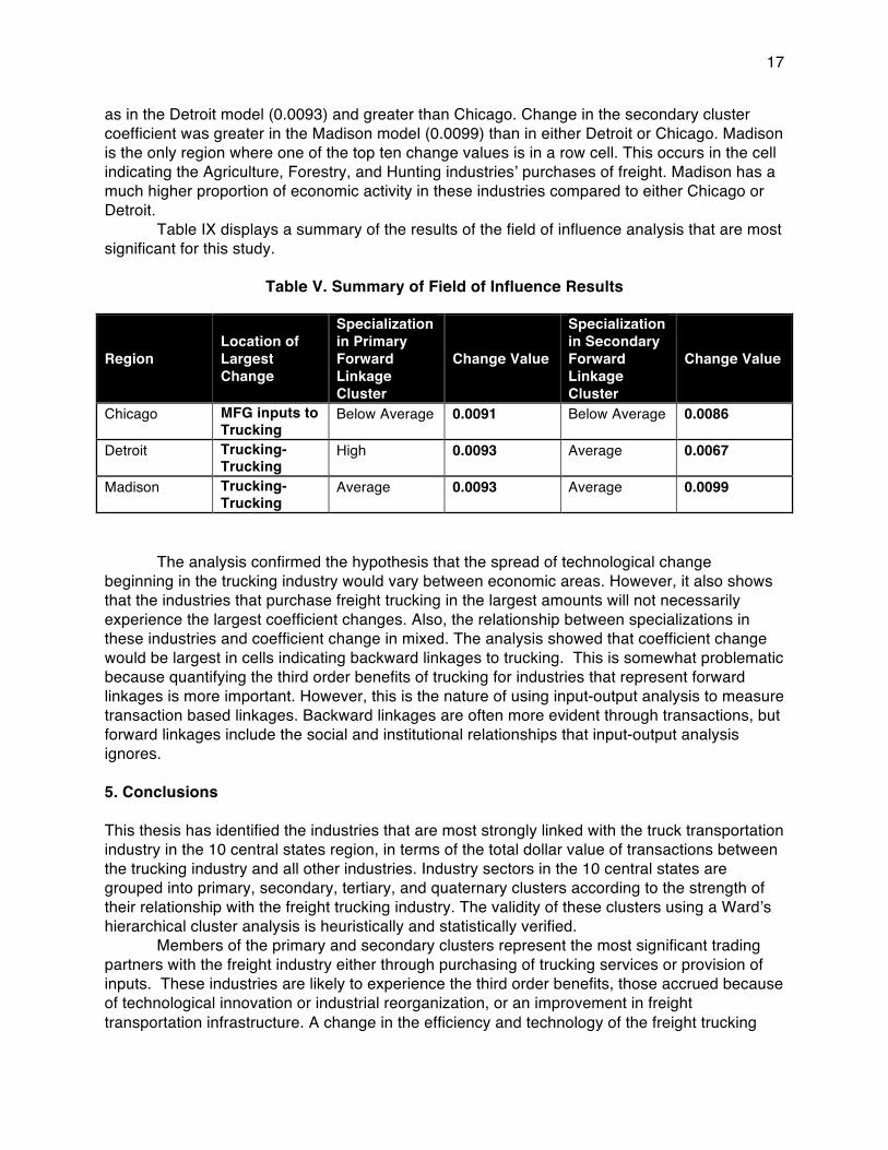
as in the Detroit model (0.0093) and greater than Chicago. Change in the secondary cluster coefficient was greater in the Madison model (0.0099) than in either Detroit or Chicago. Madison is the only region where one of the top ten change values is in a row cell. This occurs in the cell indicating the Agriculture, Forestry, and Hunting industriesʼ purchases of freight. Madison has a much higher proportion of economic activity in these industries compared to either Chicago or Detroit.

Table IX displays a summary of the results of the field of influence analysis that are most significant for this study.

Table V. Summary of Field of Influence Results

Region Location of Largest Change

Specialization in Primary Forward Linkage Cluster

Change Value

Specialization in Secondary Forward Linkage Cluster

Change Value

Chicago MFG inputs to Trucking

Below Average 0.0091 Below Average 0.0086

Detroit Trucking-Trucking

High 0.0093 Average 0.0067

Madison Trucking-Trucking

Average 0.0093 Average 0.0099

The analysis confirmed the hypothesis that the spread of technological change beginning in the trucking industry would vary between economic areas. However, it also shows that the industries that purchase freight trucking in the largest amounts will not necessarily experience the largest coefficient changes. Also, the relationship between specializations in these industries and coefficient change in mixed. The analysis showed that coefficient change would be largest in cells indicating backward linkages to trucking. This is somewhat problematic because quantifying the third order benefits of trucking for industries that represent forward linkages is more important. However, this is the nature of using input-output analysis to measure transaction based linkages. Backward linkages are often more evident through transactions, but forward linkages include the social and institutional relationships that input-output analysis ignores. 5. Conclusions This thesis has identified the industries that are most strongly linked with the truck transportation industry in the 10 central states region, in terms of the total dollar value of transactions between the trucking industry and all other industries. Industry sectors in the 10 central states are grouped into primary, secondary, tertiary, and quaternary clusters according to the strength of their relationship with the freight trucking industry. The validity of these clusters using a Wardʼs hierarchical cluster analysis is heuristically and statistically verified. Members of the primary and secondary clusters represent the most significant trading partners with the freight industry either through purchasing of trucking services or provision of inputs. These industries are likely to experience the third order benefits, those accrued because of technological innovation or industrial reorganization, or an improvement in freight transportation infrastructure. A change in the efficiency and technology of the freight trucking

18

industry should have the greatest effects on these industries. Although this study does not put forth a method to quantify the value of these third order benefits, it does point toward the industries that will experience these benefits. Location quotients are used to evaluate an economic areaʼs specialization in certain industries. This analysis shows that specialization in industries that comprise the most significant value-chain clusters for truck transportation varies across economic areas in the 10 central states. Location quotients were calculated in this study in order to provide an example metric for determining where to situate an infrastructure improvement, and to aid project analysts in explaining how an infrastructure improvement could assist the local economy. Areas that are already specialized in important industries along the value chain would receive relatively higher benefits from an infrastructure improvement in relation to their economy as a whole. This is especially true in areas specialized in forward linkage clusters because an infrastructure improvement would reduce costs to those industries and contribute to the competitiveness of a cluster of industries that contribute to the regionʼs economic base. In the long term, this might lead to improvements in resource utilization and/or innovations. Specialization means that those industries represent a relatively higher proportion of the total dollar value of output of that economic area compared to the 10 states region. Areas that are less specialized in significant industries along the value chain may want to employ infrastructure investments as a means of targeting industries that are important to freight in order to build a cluster within the region. Field of influence analysis offers the opportunity to quantify the third order benefits of infrastructure improvements. The Federal Highway Administration has already shown that infrastructure investments will alter the production process of industries in the short term using their Cost/Benefit Analysis tool. Field of influence analysis extends this evaluation to the medium to long term by modeling the spread of coefficient change throughout the entire economy as evident by changes in the Leontief inverse (total requirements) matrix.

Regional field of influence allows the economic developer or policy analysts to compare how the total impacts of an improvement in trucking technology, or efficiency, will vary by region and industry. Table IX shows that change in technology in the trucking-to-trucking cell of the input-output model (akin to a reorganization of the kind of subcontracting relationships in trucking due to increased efficiency) will change the value of the total requirement coefficient in the primary forward linkage cluster by 0.0091 in Chicago and 0.0093 in both Detroit and Madison. This means that if trucking technology were to change due to an improvement project, an increase in final demand for trucking by one dollar in either Detroit or Madison will include industries in the primary forward linkage cluster demanding 0.02 cents more per dollar of freight than industries in the primary forward linkage cluster of Chicago.

This paper has shown that regional economic structure has an effect on the diffusion of coefficient change, and thus the magnitude of the change in industry multipliers. However, attempting to place a dollar value on this magnitude to be used with cost benefit analysis may be problematic. Input-output models are accurate only for a short period of time. The technology represented in an input-output model is often out of date by the time the data become available. Additionally, projection using input-output is only applicable for the short to medium term. This is especially true in the case of infrastructure projects that alter technology because they intrinsically cause the economic structure to be altered. Input-output analysis can only work with the economic structure that is represented by the transactions matrix. The RAS method and, to a certain extent, field of influence analysis attempt to bring technological change into the model, but these extensions can only impose coefficient change mechanically based on the relationship between firms expressed in the original matrix. This does not address the issues of substitution and supply shortage that arise when attempting to make very specific projections using input-output.

19

Ethan Halpern-Givens (2010) argued in his paper that the modified RAS method would improve the accuracy of this analysis because it could reference more recent survey data to incorporate changes in interindustry relationships that have been documented since the data-year of the input-output matrix. His assessment is correct, and this study provides two methods, the clustering analysis and the field of influence analysis, for isolating the industries that should be surveyed to acquire further information. Ultimately, though, the reliability of estimates of the dollar value of third order benefits would highly variable and useful only in academic analysis. A comparison on the order of a degree of magnitude may be useful for policy analysis, but dollar value estimates are likely to vary widely from reality.

The field of influence results are more useful in comparing where infrastructure investments are likely to have the largest total effects. Policy analysts can use the new Leontief inverse matrix after a field of influence analysis to calculate new industry multipliers. Industry multipliers are based on the column sum of the total requirements matrix. All individual changes represented in the field of influence can be added up to analyze the total effect on industry multipliers. Since the assumed change of a field of influence is scalar, it would not represent a multiplier change because of a specific project, but rather it would should how sensitive total industry multipliers are to a change in trucking technology. This would allow analysts and economic developers to compare the potential magnitude of third order benefits between regions, because all spending that requires interindustry purchases, and thus is multiplied throughout the economy, will have changed due to trucking technology change. Comparing multipliers alone allows analysts to compare the potential impacts but relative to the size of the economy, similar to location quotients. Some interindusty relations may experience large multiplier change, and thus large structural impacts for the regional economy. In smaller economies, the final demand vectors will be smaller, and thus the total dollar value of this change may be lower than an economy that experiences smaller multiplier change but has a larger amount of trade. Once again, further calibration of the model in order to create this dollar value estimates is necessary. 5.1. Directions for Future Research

This study points to a number of directions for future research. I believe that the cluster analysis could be improved by including a second variable in the clustering method for both forward and backward linkages that relates the value of transactions between truck transportation and the other industries in the economy relative to total purchases/sales of other industries. Feser and Bergman (2000) use this variable in their method for determining national benchmark clusters. By using a second variable, industry relationships that are large to freight, relative to total freight purchases or output, but are not large relative to the other industry will not be similar to industry relationships that are large to freight relative to freight and the other industry.

A similar statistical study that compared the magnitude of coefficient change to the proximity of the infrastructure improvement as well as aggregate infrastructure quality would provide insightful contribution to the academic literature. Future studies could adopt an interregional input-output approach or a multiregional input-output approach in order to analyze the spillover and feedback effects resulting from infrastructure improvements.

Future research should also incorporate data available from the BEA Transportation Satellite Account in order to enhance the understanding of the transport of particular commodities. The Transportation Satellite Account provides detailed information about the distribution of trucking demand among particular commodities. This is important because it is likely that certain industries have strong linkages to freight because of the commodities that are

20

produced. This study employed a disaggregated input-output analysis in order to consider industries with as uniform output as possible, but a commodity-by-commodity input-output analysis assisted with Transportation Satellite Account data may yield significant findings.

The strategies used in this study could also be employed to analyze the role of air and rail freight transportation in order to evaluate the benefits of infrastructure improvement projects in those sectors. With different data, this analysis could be extended to other regions of the country at larger and smaller geographic levels. However, the most important research will be a detailed survey of the industries with the strongest links to transportation. It is important to have a better understanding of how different firms will respond to increased trucking efficiency in order to quantify the benefits they will accrue. The field of influence technique has proven capable of modeling the generative growth effects of transportation infrastructure investments. It is now important to calibrate this approach to account for the specificities of firm behavior that exist along the value-chain for truck transportation in order to produce a more precise accounting of third order benefits.

21

6. WORKS CITED Aldenderfer, Marc S., and Robert K. Blashfield. Cluster Analysis. Sage University Paper Series on Quantitative Applications in the Social Sciences, London, UK: Sage Pubs, 1984.

Bergman, E.M., and E.J. Feser. “Industry Clusters: A methodology and Framework for Regional Development Policy in the U.S.” In Boosting Innovation: The Cluster Approach, by T. Roelandt and P. den Herton. Paris: Organisation for Economic Cooperation and Development, 1999.

Chandra, A., and E. Thompson. “Does public infrastructure affect economic activity? Evidence from the rural interstate highway system.” Regional Science and Urban Economics 30 (2000): 457-490.

Dev Bhatta, Saurav, and Matthew P. Drennan. “The Economic Benefits of Public Investment in Transportation: A Review of Recent Literature .” The Journal of Planning Education and research, 2003: 288-296.

Feser, E. J. Benchmark value chain industry clusters for applied regional reserarch. 2005 йил 15-October. http://www.urban.illinois.edu/faculty/feser/Pubs/VC_Methods.pdf (accessed 2010 йил 1-December).

Feser, E. J., and E. M. Bergman. “National indstury cluster templates: a framework for applied regional cluster analysis.” Regional Studies 34, no. 1 (2000): 1-19.

Feser, E. J., and Michael I. Luger. “Cluster analysis as a mode of inquiry: Its use in science and technology policymaking in North Carolina.” European Planning Studies 11, no. 1 (2003): 11-24.

Feser, E. J., H. Renski, and J. Koo. Regional culster anlaysis with interindustry benchmarks. 2008 йил 7-April. http://www.urban.illinois.edufacult/feser/Pubs/TRED,%20FRK.pdf (accessed 2010 йил 1-December).

Feser, E. J., S. H. Sweeney, and H. C. Renski. “A descriptive analysis of discrete U.S. industrial complexes.” Journal of Regional Science 45, no. 2 (2005): 395-419.

Griliches, Z. “The search for R&D spillovers.” Scandinavian Journal of Economics 94 (1992): S29-S47.

Halpern-Givens, Ethan. “Evaluating the Economic Impact of Improvements in Freight Infrastructure An Input-Output Approach.” Masters Thesis. University of Illinois-Chicago, 2010.

HLB Decision Economics. Freight Benefit/Cost Study: Phase III - Analysis of Regional Benefits of Highway – Freight improvements: Final Report. The Federal Highway Adminstration, 2008.

22

HLB Decision Economics. Freight Transportation Improvements and the Economy. Report No. FHWA-HOP-04-005, Washington D.C.: U.S. Department of Transportation, Federal Highway Administration, Office of Freight Managment and Operations, 2004.

Kawamura, Kazuya, P.S. Sriraj, and Peter Lindquist. “CFIRE Grant Year 3 Research Proposal: Broad Economic Benefits of Freight Transportation Infrastructure Improvement.” 2009 йил 20-September .

Krikelas, A.C. “Why regions grow: a review of reserach on the economic base model.” Economic Review 77, no. 4 (1992): 16-21.

Leontief, Wassily. “Quantitative Input-Output Relations in the Economic System of the United States".” Review of Economics and Statistics 18, no. 3 (August 1939): 105-125.

—. The Structure of American Economy: 1919-1929. 2nd edition, 1951. New York: Oxford University Press, 1941.

MIG Inc. “Reference Manual (User's Guide to IMPLAN Version 3.0 Software).” MIG Inc. 2010 йил 30-March. http://www.implan.com/V4/index.php?option=com_multicategories&view=categories&cid=222:referencemanualusersguidetoimplanversion30software&Itemid=10 (accessed 2011 йил 11-February).

Miller, Ronald E, and Peter D. Blair. Input-Output Analysis: Foundations and Extensions . Englewood Cliffs, New Jersey: Prentice-Hall, Inc. , 1985.

Nazara, Sushasil, Doug Guo, Geoffery J.D. Hewings, and Chokri Dridi. “PyIO: Input-Output Analysis with Python- REAL 03-T-23.” The Regional Economics Applications Laboratory (REAL). 2003 йил October. http://www.real.illinois.edu/d-paper/03/03-T-23.pdf (accessed 2010 йил 8-June).

Perroux, F. “Economic space: theory and applications.” Quarterly Journal of Economics 64 (1950): 89-104.

Perroux, F. “The pole of development's new place in a general theory of economic activity.” In Regional Economic Development: Essays in Honour Francois Perroux, by Higgins B. and D. J. Savoie, 48-76. Boston, MA: Unwin Hyman, 1998.

Peters, D. J. Missouri Industry Clusters: Information Technology. Missouri Department of Economic Development, Division of Research and Planning, 2001.

Roelandt, T., J. den Hertog, J. van Sinderen, and N. van den Hove. “Cluster Analysis and Cluster-based Policy in the Netherlands.” In Boosting Innovation: The Cluster Approach, by T. Roelandt and P. den Hertog. Paris: Organisation for Economic Cooperation and Development, 1999.

23

Schumpeter, J. The Theory of Economic Development. Cambridge, MA: Harvard University Press, 1934.

Science Applications International Corporation. Freight Facts and Figures 2010. FHWA-HOP-10-058, Washington, DC: US Department of Transportation, Federal Highway Administration, Office of Freight Management and Operations, 2010.

Seetharaman, Anusha, Kazuya Kawamura, and Saurav Dev Bhatta. “Economic Benefits of Freight Policy Relating to Trucking Industry: Evaluation of Regional Transportation Plan Freight Policy for a Six-County Region, Chicago, Illinois.” Transportation Research Record , 2003: 17-23.

Sonis, Michael, and Geoffrey J.D. Hewings. Coefficient Change and Innovation Spread in Input-Output Models. Working Paper in Input-Output Economics, International Input-Output Association, 2009.

Sonis, Michael, and Geoffrey J.D. Hewings. “Economic Landscapes: Multiplier Product Matrix Analysis for Multiregional Input-Output Systems.” Hitotsubashi Journal of Economics, 1999: 59-74.

Sonis, Michael, and Geoffrey J.D. Hewings. “Fields of Influence and Extended Input-Output Analysis: A theoretical Account.” In Regional Input-Output Modelling , by John H.Li. Dewhurst, Geoffrey J.D. Hewings and Rodney C. Jensen, 141-158. Newcastle: Avebury, 1991.

Sonis, Michael, and Geoffrey J.D. Hewings. Fields of Influence in Input-Output Systems. Urbana, Ill.: Regional Economics Applications Laboratory, University of Illinois, 1994.

Sonis, Michael, Joaquim J.M. Guilhoto, Geoffrey J.D. Hewings, and Eduardo B. Martins. “Linkages, Key Sectors, and Structural Change: Some New Perspectives.” The Developing Economies, 1995: 233-270.

StatSoft. Cluster Analysis. 2008. http://www.statsoft.com/textbook/cluster-analysis/ (accessed 2011 йил 14-February).

Thompson, W. A Preface to Urban Economics. RFF, Baltimore, MD: Johns Hopkins University Press, 1965.

U.S. Department of Transportation, Federal Highway Administration. Freight Transportation: Improvements and the Economy. Report Number: FHWA-HOP-04-005, Washington, DC: U.S. Department of Transportation, Federal Highway Administration, 2004.

Ward, J. “Hierarchical grouping to optimize and objective function.” Journal of the American Statistical Association 53 (1963): 236-244.

24

25

7. Appendix A. BEA Economic Areas Aggregation EA ID EA Name Counties Included in the EA

EAs included in this study: 006 Alpena, MI Michigan: Alpena, Antrim, Charlevoix, Cheboygan, Crawford, Emmet, Montmorency,

Oscoda, Ostego, Presque Isle, Roscommon. 009 Appleton-Oshkosh-

Neenah, WI Wisconsin: Brown, Calumet, Door, Kewaunee, Menominee, Oconto, Outagamie, Shawano, Waupaca, Waushara, Winnebago.

025 Cape Girardeau-Jackson, MO-IL

Illinois: Alexander, Pulaski; Missouri: Bollinger, Butler, Cape Girardeau, Carter, Mississippi, New Madrid, Perry, Ripley, Scott, Stoddard, Wayne.

027 Cedar Rapids, IA Iowa: Benton, Cedar, Iowa, Johnson, Jones, Keokuk, Linn, Louisa, Muscatine, Washington.

028 Champaign-Urbana, IL

Illinois: Champaign, Clay, Coles, Cumberland, Douglas, Effingham, Fayette, Ford, Jasper, Moultrie, Piatt, Richland, Shelby, Vermilion, Wayne.

032 Chicago-Naperville-Michigan City, IL-IN-WI

Illinois: Boone, Bureau, Carroll, Cook, DeKalb, DuPage, Grundy, Iroquois, Kane, Kankakee, Kendall, Lake, LaSalle, Lee, Livingston, McHenry, Ogle, Putnam, Stephenson, Will, Winnebago; Indiana: Jasper, Lake, LaPorte, Newton, Porter; Wisconsin: Kenosha.

033 Cincinnati-Middletown-Wilmington, OH-KY-IN

Indiana: Dearborn, Franklin, Ohio, Ripley, Switzerland; Kentucky: Boone, Bracken, Campbell, Fleming, Gallatin, Grant, Kenton, Lewis, Mason, Owen, Pendleton; Ohio: Adams, Brown, Butler, Clermont, Clinton, Hamilton, Highland, Warren.

035 Cleveland-Akron-Elyria, OH

Ohio: Ashland, Ashtabula, Carroll, Columbiana, Crawford, Cuyahoga, Erie, Geauga, Harrison, Holmes, Huron, Lake, Lorain, Mahoning, Medina, Portage, Richland, Stark, Summit, Trumbull, Tuscarawas, Wayne; Pennsylvania: Mercer.a

037 Columbia, MO Missouri: Audrain, Boone, Callaway, Camden, Cole, Cooper, Howard, Maries, Miller, Moniteau, Monroe, Morgan, Osage, Randolph, Shelby.

040 Columbus-Marion-Chillicothe, OH

Ohio: Athens, Coshocton, Delaware, Fairfield, Fayette, Franklin, Gallia, Guernsey, Hardin, Hocking, Jackson, Knox, Licking, Logan, Madison, Marion, Meigs, Morgan, Morrow, Muskingum, Noble, Perry, Pickaway, Pike, Ross, Scioto, Union, Vinton; West Virginia: Mason.b

043 Davenport-Moline-Rock Island, IA-IL

Illinois: Henry, Mercer, Rock Island, Whiteside; Iowa: Clinton, Scott.

044 Dayton-Springfield-Greenville, OH

Ohio: Allen, Auglaize, Champaign, Clark, Darke, Greene, Mercer, Miami, Montgomery, Preble, Putnam, Shelby, Van Wert.

046 Des Moines-Newton-Pella, IA

Iowa: Adair, Adams, Appanoose, Boone, Buena Vista, Calhoun, Carroll, Cherokee, Clarke, Clay, Crawford, Dallas, Davis, Decatur, Dickinson, Emmet, Franklin, Greene, Guthrie, Hamilton, Hardin, Humboldt, Ida, Jasper, Lucas, Madison, Mahaska, Marion, Marshall, Monroe, Palo Alto, Pocahontas, Polk, Poweshiek, Ringgold, Sac, Story, Tama, Union, Wapello, Warren, Wayne, Webster, Wright.

047 Detroit-Warren-Flint, MI

Michigan: Alcona, Arenac, Bay, Clare, Clinton, Eaton, Genesee, Gladwin, Gratiot, Hillsdale, Huron, Ingham, Iosco, Isabella, Jackson, Lapeer, Lenawee, Livingston, Macomb, Midland, Monroe, Oakland, Ogemaw, Saginaw, St. Clair, Sanilac, Shiawassee, Tuscola, Washtenaw, Wayne.

050 Duluth, MN-WI Minnesota: Carlton, Cook, Itasca, Koochiching, Lake, St. Louis; Wisconsin: Douglas. 054 Evansville, IN-KY Illinois: Edwards, Gallatin, Wabash, White; Indiana: Daviess, Dubois, Gibson, Martin,

Perry, Pike, Posey, Spencer, Vanderburgh, Warrick; Kentucky: Daviess, Hancock, Henderson, Hopkins, McLean, Muhlenberg, Ohio, Union, Webster.

060 Fort Wayne-Huntington-Auburn, IN

Indiana: Adams, Allen, Blackford, DeKalb, Grant, Huntington, Jay, Noble, Steuben, Wabash, Wells, Whitley; Michigan: Branch.

064 Grand Rapids-Muskegon-Holland, MI

Michigan: Allegan, Barry, Calhoun, Ionia, Kalamazoo, Kent, Mecosta, Montcalm, Muskegon, Newaygo, Oceana, Ottawa, Van Buren.

BEA Economic Areas (continued)

26

EA ID EA Name Counties Included in the EA

078 Indianapolis-Anderson-Columbus, IN

Illinois: Clark, Crawford, Edgar, Lawrence; Indiana: Bartholomew, Benton, Boone, Brown, Carroll, Cass, Clay, Clinton, Decatur, Delaware, Fayette, Fountain, Greene, Hamilton, Hancock, Hendricks, Henry, Howard, Jackson, Jennings, Johnson, Knox, Lawrence, Madison, Marion, Miami, Monroe, Montgomery, Morgan, Orange, Owen, Parke, Putnam, Randolph, Rush, Shelby, Sullivan, Tippecanoe, Tipton, Union, Vermillion, Vigo, Warren, Wayne, White.

083 Joplin, MO Kansas: Allen, Bourbon, Cherokee, Crawford, Neosho, Wilson, Woodson; Missouri: Barton, Cedar, Jasper, Newton, Vernon; Oklahoma: Ottawa.b

084 Kansas City-Overland Park-Kansas City, MO-KS

Kansas: Anderson, Atchison, Doniphan, Douglas, Franklin, Johnson, Leavenworth, Linn, Miami, Wyandotte; Missouri: Adair, Andrew, Bates, Benton, Buchanan, Caldwell, Carroll, Cass, Chariton, Clay, Clinton, Daviess, DeKalb, Gentry, Grundy, Harrison, Henry, Holt, Jackson, Johnson, Knox, Lafayette, Linn, Livingston, Macon, Mercer, Nodaway, Pettis, Platte, Putnam, Ray, St. Clair, Saline, Schuyler, Sullivan, Worth.

089 La Crosse, WI-MN Minnesota: Houston; Wisconsin: Jackson, La Crosse, Monroe, Trempealeau, Vernon. 094 Lexington-Fayette-

Frankfort-Richmond, KY

Kentucky: Anderson, Bath, Bourbon, Boyle, Breathitt, Casey, Clark, Clay, Clinton, Cumberland, Elliot, Estill, Fayette, Floyd, Franklin, Garrard, Harlan, Harrison, Jackson, Jessamine, Johnson, Knott, Knox, Laurel, Lee, Leslie, Letcher, Lincoln, McCreary, Madison, Magoffin, Martin, Menifee, Mercer, Montgomery, Morgan, Nicholas, Owsley, Perry, Pike, Powell, Pulaski, Robertson, Rockcastle, Rowan, Russell, Scott, Washington, Wayne, Whitley, Wolfe, Woodford; West Virginia: Mingo. b

098 Louisville-Elizabethtown-Scottsburg, KY-IN

Indiana: Clarke, Crawford, Floyd, Harrison, Jefferson, Scott, Washington; Kentucky: Adair, Breckinridge, Bullitt, Carroll, Grayson, Green, Hardin, Henry, Jefferson, Larue, Marion, Meade, Nelson, Oldham, Shelby, Spencer, Taylor, Trimble.

101 Madison-Baraboo, WI

Illinois: Jo Daviess; Iowa: Allamakee, Clayton, Delaware, Dubuque, Jackson; Wisconsin: Adams, Columbia, Crawford, Dane, Grant, Green, Iowa, Juneau, Lafayette, Marquette, Richland, Rock, Sauk.

102 Marinette, WI-MI Michigan: Alger, Baraga, Chippewa, Delta, Dickinson, Houghton, Iron, Keweenaw, Luce, Mackinac, Marquette, Menominee, Schoolcraft; Wisconsin: Florence, Marinette.

103 Mason City, IA Iowa: Cerro Gordo, Chickasaw, Floyd, Hancock, Howard, Kossuth, Mitchell, Winnebago, Winneshiek, Worth.

108 Milwaukee-Racine-Waukesha, WI

Wisconsin: Dodge, Fond du Lac, Green Lake, Jefferson, Manitowoc, Milwaukee, Ozaukee, Racine, Sheboygan, Walworth, Washington, Waukesha.

109 Minneapolis-St. Paul-St. Cloud, MN-WI

Minnesota: Aitkin, Anoka, Becker, Beltrami, Benton, Big Stone, Blue Earth, Brown, Carver, Cass, Chippewa, Chisago, Clearwater, Cottonwood, Crow Wing, Dakota, Dodge, Douglas, Faribault, Fillmore, Freeborn, Goodhue, Grant, Hennepin, Hubbard, Isanti, Jackson, Kanabec, Kandiyohi, Lac qui Parle, Le Sueur, Lincoln, Lyon, McLeod, Mahnomen, Martin, Meeker, Mille Lacs, Morrison, Mower, Murray, Nicollet, Olmsted, Otter Tail, Pine, Pope, Ramsey, Redwood, Renville, Rice, Scott, Sherburne, Sibley, Stearns, Steele, Stevens, Swift, Todd, Traverse, Wabasha, Wadena, Waseca, Washington, Watonwan, Winona, Wright, Yellow Medicine; South Dakota: Grant,b Marshall,b Roberts;b Wisconsin: Barron, Buffalo, Burnett, Chippewa, Dunn, Eau Claire, Pepin, Pierce, Polk, Rusk, St. Croix, Sawyer, Washburn.

122 Paducah, KY-IL Illinois: Massac, Pope; Kentucky: Ballard, Caldwell, Calloway, Carlisle, Crittenden, Graves, Livingston, Lyon, McCracken, Marshall.

126 Peoria-Canton, IL Illinois: De Witt, Fulton, Hancock, Henderson, Knox, McDonough, McLean, Marshall, Mason, Peoria, Stark, Tazewell, Warren, Woodford; Iowa: Des Moines, Henry, Jefferson, Lee, Van Buren; Missouri: Clark, Scotland.

141 Salina, KS Kansas: Cheyenne, Cloud, Decatur, Ellis, Ellsworth, Gove, Graham, Jewell, Lincoln, Logan, Mitchell, Norton, Osborne, Ottawa, Phillips, Rawlins, Republic, Rooks, Russell, Saline, Sheridan, Sherman, Smith, Thomas, Trego, Wallace.

156 South Bend-Mishawaka, IN-MI

Indiana: Elkhart, Fulton, Kosciusko, Lagrange, Marshall, Pulaski, St. Joseph, Starke; Michigan: Berrien, Cass, St. Joseph.

158 Springfield, IL Illinois: Adams, Brown, Cass, Christian, Greene, Logan, Macon, Menard, Montgomery, Morgan, Pike, Sangamon, Schuyler, Scott; Missouri: Lewis, Marion, Ralls.

159 Springfield, MO Arkansas: Baxter,b Boone,b Carroll,b Marion,b Newton;b Missouri: Barry, Christian, Dade, Dallas, Bent, Douglas, Greene, Hickory, Howell, Laclede, Lawrence, Oregon,

27

Ozark, Phelps, Polk, Pulaski, Shannon, Stone, Taney, Texas, Webster, Wright. BEA Economic Areas (continued)

EA ID EA Name Counties Included in the EA

160 St. Louis-St. Charles-Farmington, MO-IL

Illinois: Bond, Calhoun, Clinton, Franklin, Hamilton, Hardin, Jackson, Jefferson, Jersey, Johnson, Macoupin, Madison, Marion, Monroe, Perry, Randolph, St. Clair, Saline, Union, Washington, Williamson; Missouri: Crawford, Franklin, Gasconade, Iron, Jefferson, Lincoln, Madison, Montgomery, Pike, Reynolds, St. Charles, Ste. Genevieve, St. Francois, St. Louis, Warren, Washington, St. Louis (Independent City).

166 Toledo-Fremont, OH Ohio: Defiance, Fulton, Hancock, Henry, Lucas, Ottawa, Paulding, Sandusky, Seneca, Williams, Wood, Wyandot.

167 Topeka, KS Kansas: Brown, Chase, Clay, Coffey, Dickinson, Geary, Jackson, Jefferson, Lyon, Marshall, Morris, Nemaha, Osage, Pottawatomie, Riley, Shawnee, Wabaunsee, Washington.

168 Traverse City, MI Michigan: Benzie, Grand Traverse, Kalkaska, Lake, Leelanau, Manistee, Mason, Missaukee, Osceola, Wexford.

175 Waterloo-Cedar Falls, IA

Iowa: Black Hawk, Bremer, Buchanan, Butler, Fayette, Grundy.

176 Wausau-Merrill, WI Michigan: Gogebic, Ontonagon; Wisconsin: Ashland, Bayfield, Clark, Forest, Iron, Langlade, Lincoln, Marathon, Oneida, Portage, Price, Taylor, Vilas, Wood.

179 Wichita-Winfield, KS Kansas: Barber, Barton, Butler, Chautauqua, Clark, Comanche, Cowley, Edwards, Elk, Finney, Ford, Grant, Gray, Greeley, Greenwood, Hamilton, Harper, Harvey, Haskell, Hodgeman, Kearny, Kingman, Kiowa, Labette, Lane, McPherson, Marion, Montgomery, Ness, Pawnee, Pratt, Reno, Rice, Rush, Scott, Sedgwick, Stafford, Stanton, Sumner, Wichita; Oklahoma: Kay.b

EAs excluded from this study: 029 Charleston, WV Kentucky: Boyd, Carter, Greenup, Lawrence; Ohio: Lawrence, Washington; West

Virginia: Boone, Braxton, Cabell, Calhoun, Clay, Fayette, Gilmer, Greenbrier, Jackson, Kanawha, Lincoln, Logan, Nicholas, Pleasants, Pocahontas, Putnam, Raleigh, Randolph, Ritchie, Roane, Summers, Tucker, Wayne, Webster, Wirt, Wood, Wyoming.

055 Fargo-Wahpeton, ND-MN

Minnesota: Clay, Norman, Wilkin; North Dakota: Barnes, Cass, Dickey, Foster, Griggs, LaMoure, Ransom, Richland, Sargent, Sheridan, Stutsman, Wells.

057 Fayetteville-Springdale-Rogers, AR-MO

Arkansas: Benton, Madison Washington; Missouri: McDonald; Oklahoma: Adair, Delaware.

063 Grand Forks, ND-MN

Minnesota: Kittson, Lake of the Woods, Marshall, Pennington, Polk, Red Lake, Roseau; North Dakota: Benson, Cavalier, Eddy, Grand Forks, Nelson, Pembina, Ramsey, Steele, Traill, Walsh.

082 Jonesboro, AR Arkansas: Clay, Craighead, Greene, Lawrence, Mississippi, Poinsett, Randolph; Missouri: Dunklin, Pemiscot.

116 Nashville-Davidson-Murfresboro-Columbia, TN

Kentucky: Allen, Barren, Butler, Christian, Edmonson, Hart, Logan, Metcalfe, Monroe, Simpson, Todd, Trigg, Warren; Tennessee: Bedford, Cannon, Cheatham, Clay, Coffee, Cumberland, Davidson, DeKalb, Dickson, Fentress, Franklin, Giles, Grundy, Hickman, Houston, Humphreys, Jackson, Lawrence, Lewis, Macon, Marshall, Maury, Montgomery, Moore, Overton, Perry, Pickett, Putnam, Robertson, Rutherford, Smith, Stewart, Sumner, Trousdale, Van Buren, Warren, Wayne, White, Williamson, Wilson.

119 Oklahoma City-Shawnee, OK

Kansas: Meade, Morton, Seward, Stevens; Oklahoma: Alfalfa, Beaver, Beckham, Blaine, Caddo, Canadian, Carter, Cimarron, Cleveland, Coal, Comanche, Cotton, Custer, Dewey, Ellis, Garfield, Garvin, Grady, Grant, Greer, Harmon, Harper, Hughes, Jackson, Jefferson, Johnston, Kingfisher, Kiowa, Lincoln, Logan, Love, McClain, Major, Marshall, Murray, Oklahoma, Pontotoc, Pottawatomie, Roger Mills, Seminole, Stephens, Texas, Tillman, Washita, Woods, Woodward; Texas: Sherman.

120 Omaha-Council Bluffs-Fremont, NE-IA

Iowa: Audubon, Cass, Fremont, Harrison, Mills, Montgomery, Page, Pottawattamie, Shelby, Taylor; Missouri: Atchison; Nebraska: Boone, Burt, Butler, Cass, Colfax, Cuming, Dodge, Douglas, Nance, Platte, Polk, Sarpy, Saunders, Washington.

129 Pittsburgh-New Castle, PA

Ohio: Belmont, Jefferson, Monroe; Pennsylvania: Allegheny, Armstrong, Beaver, Butler, Fayette, Greene, Indiana, Lawrence, Washington, Westmoreland; West Virginia: Brooke, Hancock, Marshall, Ohio, Tyler, Wetzel.

28

154 Sioux City-Vermillion, IA-NE-SD

Iowa: Monona, OʼBrien, Osceola, Plymouth, Sioux, Woodbury; Nebraska: Antelope, Boyd, Cedar Dakota, Dixon, Holt, Knox, Madison, Pierce, Stanton, Thurston, Wayne, Wheeler; South Dakota: Bon Homme, Clay, Union, Yankton.

BEA Economic Areas (continued) EA ID EA Name Counties Included in the EA

155 Sioux Falls, SD Iowa: Lyon; Minnesota: Nobles, Pipestone, Rock; South Dakota: Aurora, Beadle, Brookings, Brule, Buffalo, Charles Mix, Clark, Codington, Davison, Day Deuel, Douglas, Hamlin, Hand, Hanson, Hughes, Hutchinson, Hyde, Jerauld, Jones, Kingsbury, Lake, Lincoln, Lyman, McCook, Miner, Minnehaha, Moody, Sanborn, Stanley, Sully, Turner.

a Data for this county were available, and the county was included in the EA. b Data for this county were not available. This county was excluded from the EA for the purpose of this study.

29

8. Appendix B Chebychev Distance

Chebychev distance between cases and is defined as:

where is the maximum of the absolute difference between cases and across all

clustering variables.

Wardʼs Method

The within-groups sum of squares, or error sum of squares (ESS) is:

where is the score of the case.

30

9. Appendix C. Forward Linkage Clusters Continued

Cluster Code Description Total Output 3 65 Snack food manufacturing $183,625,388 3 138 Soap and cleaning compound manufacturing $177,716,891 3 133 Pharmaceutical preparation manufacturing $177,221,740 3 427 US Postal Service $176,508,408 3 113 Printing $175,655,471 3 71 Breweries $166,472,447 3 115 Petroleum refineries $159,303,260 3 60 Poultry processing $158,883,315 3 205 Construction machinery manufacturing $158,527,631 3 318 Broom, brush, and mop manufacturing $158,010,930 3 57 Dry, condensed, and evaporated dairy product manufacturing $156,547,937 3 108 Coated and laminated paper, packaging paper and plastics film

manufacturing $154,215,646

3 323 Retail Stores - Building material and garden supply $149,028,491 3 177 Copper rolling, drawing, extruding and alloying $145,026,301 3 174 Aluminum product manufacturing from purchased aluminum $144,140,159 3 21 Mining coal $143,253,154 3 43 Flour milling and malt manufacturing $135,371,684 3 374 Management, scientific, and technical consulting services $134,356,776 3 305 Surgical and medical instrument, laboratory and medical instrument

manufacturing $133,376,956

3 168 Mineral wool manufacturing $132,174,923 3 47 Breakfast cereal manufacturing $131,186,975 3 285 Aircraft engine and engine parts manufacturing $128,768,115 3 69 All other food manufacturing $127,392,762 3 186 Plate work and fabricated structural product manufacturing $125,627,366 3 25 Mining and quarrying stone $124,150,743 3 172 Alumina refining and primary aluminum production $122,785,173 3 187 Ornamental and architectural metal products manufacturing $122,102,780 3 333 Transport by rail $121,005,780 3 12 Dairy cattle and milk production $120,574,435 3 325 Retail Stores - Health and personal care $120,516,152 3 190 Metal can, box, and other metal container (light gauge) manufacturing $119,991,079 3 351 Telecommunications $119,376,881 3 111 Sanitary paper product manufacturing $118,651,655 3 13 Poultry and egg production $118,422,287 3 228 Material handling equipment manufacturing $118,005,956 3 95 Sawmills and wood preservation $115,518,297 3 284 Aircraft manufacturing $114,846,260 3 295 Wood kitchen cabinet and countertop manufacturing $110,801,742 3 331 Retail Nonstores - Direct and electronic sales $110,530,409 3 40 Maintenance and repair construction of residential structures $108,279,191 3 73 Distilleries $106,053,422 3 14 Animal production, except cattle and poultry and eggs $102,955,185 3 341 Newspaper publishers $102,256,450 3 63 Cookie, cracker, and pasta manufacturing $98,457,596 3 306 Surgical appliance and supplies manufacturing $95,724,988 3 197 Coating, engraving, heat treating and allied activities $95,509,135 3 68 Seasoning and dressing manufacturing $93,461,166

Forward Linkage Clusters (continued)

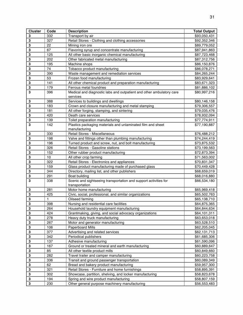
31

Cluster Code Description Total Output 3 332 Transport by air $93,050,431 3 327 Retail Stores - Clothing and clothing accessories $92,352,346 3 22 Mining iron ore $89,779,052 3 67 Flavoring syrup and concentrate manufacturing $87,941,863 3 125 All other basic inorganic chemical manufacturing $87,723,468 3 202 Other fabricated metal manufacturing $87,312,756 3 195 Machine shops $86,150,876 3 74 Tobacco product manufacturing $86,078,271 3 390 Waste management and remediation services $84,265,244 3 53 Frozen food manufacturing $83,929,641 3 141 All other chemical product and preparation manufacturing $83,671,323 3 179 Ferrous metal foundries $81,886,102 3 396 Medical and diagnostic labs and outpatient and other ambulatory care

services $80,997,216

3 388 Services to buildings and dwellings $80,146,158 3 183 Crown and closure manufacturing and metal stamping $79,306,557 3 181 All other forging, stamping, and sintering $79,035,476 3 420 Death care services $78,932,094 3 139 Toilet preparation manufacturing $77,774,911 3 142 Plastics packaging materials and unlaminated film and sheet

manufacturing $77,190,887

3 330 Retail Stores - Miscellaneous $76,488,212 3 198 Valve and fittings other than plumbing manufacturing $74,244,419 3 196 Turned product and screw, nut, and bolt manufacturing $73,875,532 3 326 Retail Stores - Gasoline stations $73,199,563 3 152 Other rubber product manufacturing $72,873,394 3 10 All other crop farming $71,563,002 3 322 Retail Stores - Electronics and appliances $70,831,347 3 159 Glass product manufacturing made of purchased glass $70,449,428 3 344 Directory, mailing list, and other publishers $68,659,019 3 291 Boat building $68,016,880 3 338 Scenic and sightseeing transportation and support activities for

transportation $66,534,180

3 281 Motor home manufacturing $65,969,418 3 425 Civic, social, professional, and similar organizations $65,502,763 3 1 Oilseed farming $65,138,710 3 398 Nursing and residential care facilities $64,875,365 3 264 Household laundry equipment manufacturing $64,844,634 3 424 Grantmaking, giving, and social advocacy organizations $64,101,311 3 278 Heavy duty truck manufacturing $63,653,018 3 267 Motor and generator manufacturing $63,528,510 3 106 Paperboard Mills $62,205,045 3 377 Advertising and related services $62,131,713 3 342 Periodical publishers $61,685,306 3 137 Adhesive manufacturing $61,590,096 3 167 Ground or treated mineral and earth manufacturing $60,889,647 3 85 All other textile product mills $60,849,660 3 282 Travel trailer and camper manufacturing $60,223,758 3 336 Transit and ground passenger transportation $60,089,349 3 62 Bread and bakery product manufacturing $59,957,300 3 321 Retail Stores - Furniture and home furnishings $58,895,391 3 302 Showcase, partition, shelving, and locker manufacturing $58,823,678 3 194 Spring and wire product manufacturing $58,807,159 3 230 Other general purpose machinery manufacturing $56,553,483

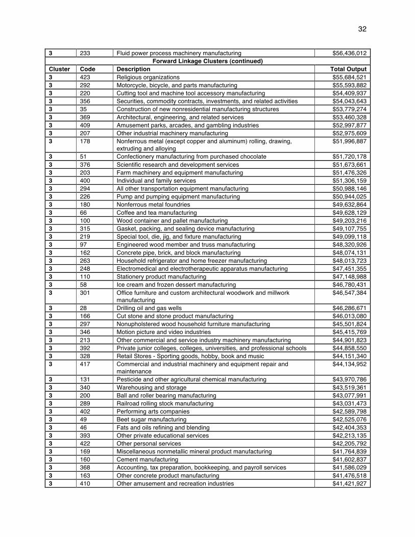
32

3 233 Fluid power process machinery manufacturing $56,436,012 Forward Linkage Clusters (continued)

Cluster Code Description Total Output 3 423 Religious organizations $55,684,521 3 292 Motorcycle, bicycle, and parts manufacturing $55,593,882 3 220 Cutting tool and machine tool accessory manufacturing $54,409,937 3 356 Securities, commodity contracts, investments, and related activities $54,043,643 3 35 Construction of new nonresidential manufacturing structures $53,779,274 3 369 Architectural, engineering, and related services $53,460,328 3 409 Amusement parks, arcades, and gambling industries $52,997,877 3 207 Other industrial machinery manufacturing $52,975,609 3 178 Nonferrous metal (except copper and aluminum) rolling, drawing,

extruding and alloying $51,996,887

3 51 Confectionery manufacturing from purchased chocolate $51,720,178 3 376 Scientific research and development services $51,673,661 3 203 Farm machinery and equipment manufacturing $51,476,326 3 400 Individual and family services $51,306,159 3 294 All other transportation equipment manufacturing $50,988,146 3 226 Pump and pumping equipment manufacturing $50,944,025 3 180 Nonferrous metal foundries $49,632,864 3 66 Coffee and tea manufacturing $49,628,129 3 100 Wood container and pallet manufacturing $49,203,216 3 315 Gasket, packing, and sealing device manufacturing $49,107,755 3 219 Special tool, die, jig, and fixture manufacturing $49,099,118 3 97 Engineered wood member and truss manufacturing $48,320,926 3 162 Concrete pipe, brick, and block manufacturing $48,074,131 3 263 Household refrigerator and home freezer manufacturing $48,013,723 3 248 Electromedical and electrotherapeutic apparatus manufacturing $47,451,355 3 110 Stationery product manufacturing $47,148,988 3 58 Ice cream and frozen dessert manufacturing $46,780,431 3 301 Office furniture and custom architectural woodwork and millwork

manufacturing $46,547,384

3 28 Drilling oil and gas wells $46,286,671 3 166 Cut stone and stone product manufacturing $46,013,080 3 297 Nonupholstered wood household furniture manufacturing $45,501,824 3 346 Motion picture and video industries $45,415,769 3 213 Other commercial and service industry machinery manufacturing $44,901,823 3 392 Private junior colleges, colleges, universities, and professional schools $44,858,550 3 328 Retail Stores - Sporting goods, hobby, book and music $44,151,340 3 417 Commercial and industrial machinery and equipment repair and

maintenance $44,134,952

3 131 Pesticide and other agricultural chemical manufacturing $43,970,786 3 340 Warehousing and storage $43,519,361 3 200 Ball and roller bearing manufacturing $43,077,991 3 289 Railroad rolling stock manufacturing $43,031,473 3 402 Performing arts companies $42,589,798 3 49 Beet sugar manufacturing $42,525,076 3 46 Fats and oils refining and blending $42,404,353 3 393 Other private educational services $42,213,135 3 422 Other personal services $42,205,792 3 169 Miscellaneous nonmetallic mineral product manufacturing $41,764,839 3 160 Cement manufacturing $41,602,837 3 368 Accounting, tax preparation, bookkeeping, and payroll services $41,586,029 3 163 Other concrete product manufacturing $41,476,518 3 410 Other amusement and recreation industries $41,421,927

33

3 26 Mining and quarrying sand, gravel, clay, and ceramic and refractory minerals

$41,198,357

3 261 Small electrical appliance manufacturing $40,535,892 Forward Linkage Clusters (continued)

Cluster Code Description Total Output 3 317 All other miscellaneous manufacturing $40,494,558 3 240 Audio and video equipment manufacturing $40,210,596 3 367 Legal services $40,063,248 3 357 Insurance carriers $39,891,713 3 334 Transport by water $39,842,154 3 150 Tire manufacturing $39,626,729 3 279 Motor vehicle body manufacturing $39,426,578 3 109 All other paper bag and coated and treated paper manufacturing $39,062,517 3 339 Couriers and messengers $38,892,954 3 246 Printed circuit assembly (electronic assembly) manufacturing $38,790,098 4 --- ALL OTHER INDUSTRIES $3,380,321,499

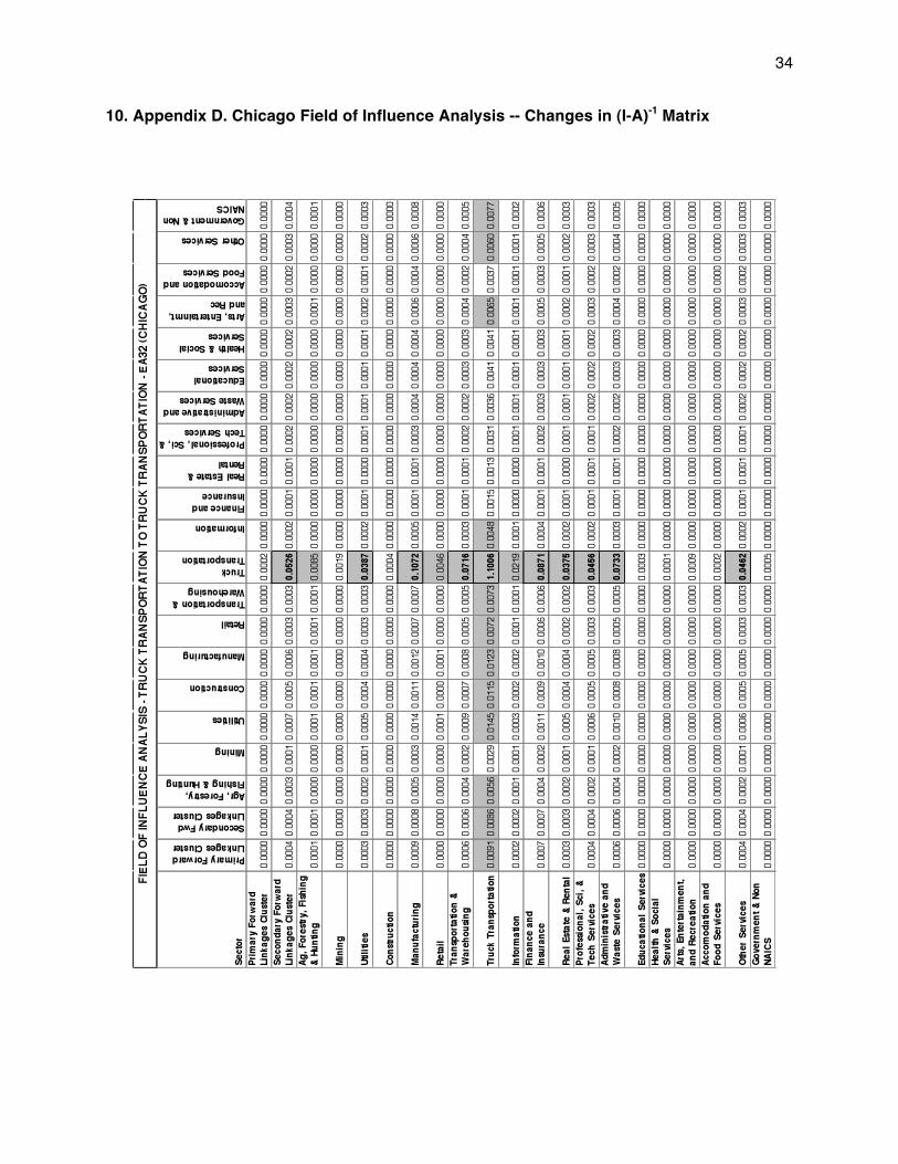
34

10. Appendix D. Chicago Field of Influence Analysis -- Changes in (I-A)-1 Matrix