Embed Size (px)
Citation preview

DEPARTMENT OF ECONOMICS, UPPSALA UNIVERSITY
Evaluating the potential profitability of alpha trading
Author: Ellinor Gyldberg
Supervisor: Mikael Bask
17/1 2019
The purpose of this thesis is to test whether an active trading strategy using historical alpha values (a
measure of risk-adjusted excess returns) for stocks can be used to achieve positive risk-adjusted profits.
To do so, data on stocks in the Dow Jones Industrial Average and the Standard & Poor’s 500 Index from
1997 to 2018 are used to estimate the market model, using GARCH and TGARCH. Three kinds of
portfolios are evaluated: portfolios to be held long, consisting of stocks with historical alpha values
estimated to be larger than zero; portfolios to be held short, consisting of stocks with historical alpha
values estimated to be less than zero; and self-financing portfolios, where stocks that have positive
historical risk-adjusted returns are held long but stocks that have historical negative risk-adjusted
returns are held short. The results of this study indicate that this trading strategy does not
systematically “beat the market”.

2
CONTENTS
1. Introduction ............................................................................................................................................................................ 3
2. Theoretical framework ...................................................................................................................................................... 6
2.1. The Capital Asset Pricing Model ............................................................................................................................ 6
2.2. Jensen’s alpha ................................................................................................................................................................ 8
2.3. The Efficient Market Hypothesis ........................................................................................................................... 8
2.4. Sharpe ratio .................................................................................................................................................................... 9
3. Previous studies ................................................................................................................................................................. 10
4. Data ......................................................................................................................................................................................... 12
4.1. Stocks and market index data .............................................................................................................................. 12
4.1.1. Stocks excluded from the sample .............................................................................................................. 16
4.2. Risk-free rate .............................................................................................................................................................. 17
5. Empirical Method .............................................................................................................................................................. 17
5.1. Portfolio creation ...................................................................................................................................................... 19
5.2. The GARCH and TGARCH models ....................................................................................................................... 23
6. Results .................................................................................................................................................................................... 28
6.1 Whole period, using GARCH .................................................................................................................................. 29
6.2 Whole period, using TGARCH ............................................................................................................................... 33
6.3 Post-crisis period, using GARCH .......................................................................................................................... 37
6.4 Post-crisis period, using TGARCH ....................................................................................................................... 41
7. Discussion ............................................................................................................................................................................. 45
References ................................................................................................................................................................................. 47
Articles ................................................................................................................................................................................... 47
Webpages ............................................................................................................................................................................. 50

3
1. INTRODUCTION
The purpose of this thesis is to test whether an active trading strategy, where we invest in stocks
with positive historical risk-adjusted profits, would have been successful had it been used between
2007 and 2018 in the US stock market.
The question of evaluating active trading strategies is central to the field of finance as it is essential
for investors to know if it is worth investing their time and resources in an active trading strategy
rather than passive investment strategies. If ways to use active trading strategies to systematically
achieve abnormal profits exist, they create an incentive for investors to choose active investment
strategies. This is closely related to the concept of weak-form market efficiency, which means that
historical price developments and traded volumes are reflected in current asset prices. If weak-form
market efficiency holds, this would imply that there are no possibilities to use this data to formulate
an investment strategy which would beat the market.
Intuitively, it seems implausible that a trading strategy based on an expectation of positive
autocorrelation in stock returns would produce abnormal profits because of its simplicity and
availability to all investors. However, in their bachelor’s thesis from 2017, Funke & Sinjari found
that using this type of trading strategy on the Swedish stock market would have generated a
significant positive risk-adjusted profit compared to the OMXS30 index. Although this result might
be due to chance, it still suggests that this type of trading strategy could be worth a second look.
In this thesis, we test how this trading strategy would have performed in the US market. In order to
do so, we use monthly adjusted close data from 1997 to 2018 on the Dow Jones Industrial Average
Index, the Standard & Poor’s 500 Index, and individual stocks in the Dow Jones Industrial Average.
Because the adjusted close price takes dividends and splits into account, reflecting the investor’s
profit better than the close price, it makes sense to use the adjusted close price when evaluating an
active trading strategy.
In this thesis, eleven different datasets are used to test whether portfolios created using this
strategy outperform the market. This is done by estimating the market model using either a GARCH
or a threshold-asymmetric GARCH (TGARCH) model for the error term. The reason why GARCH and
TGARCH are used is because the OLS assumption of homoscedasticity is not fulfilled for financial

4
time series. Volatility clustering, a form of conditional heteroscedasticity, is a common characteristic
of financial data, and extreme events are common enough for the Student’s t-distribution to be a
better fit than the normal distribution. GARCH and TGARCH are well-equipped to handle conditional
heteroscedasticity as well as the “fat tails” produced by volatility clustering.
Had OLS been used while heteroscedasticity is present, we would risk inefficient estimators, a
higher type 1 error than the selected significance level, and a downwards bias in our estimate of the
coefficient of determination. An estimate of the coefficient of determination which is lower than the
true value implies an understated systematic risk and an overstated diversifiable risk. If the type 1
error does not match the desired significance level, we risk making incorrect inferences. Using
GARCH-type models takes care of these issues.
Portfolios are created using the last ten years’ returns to estimate historical alpha values, and each
portfolio is then rebalanced every year, using the composition of the Dow Jones Industrial Average
at the time of rebalancing. The measurements used for the evaluation of these strategies are the
alpha value of the portfolio, the Sharpe ratio, and the change of the portfolio’s value from the
beginning to the end of the evaluation period. The alpha value is a measurement of the risk-adjusted
return compared to the market index. The Sharpe ratio describes how much excess return you
receive for the extra volatility that you tolerate when holding a riskier asset. These are two of the
most common ways to measure risk-adjusted returns, and together with the value change of the
portfolios, they give us a comprehensive view of how the performances of the portfolios differ in
terms of both absolute return and risk-adjusted return.
We find that using alpha trading in the US market would not have produced positive risk-adjusted
profits. For the evaluation done using the whole period, the portfolios held short decreased in value,
whereas the portfolios held long increased in value. However, when we evaluate this trading
strategy using only the period after the financial crisis, we instead find that the portfolios held short
sometimes have the greatest value increases. We also see a relationship between a stock having
significantly positive historical alpha values (at the 5% level) and a higher future volatility. All
estimated alpha values are close to zero, so the investor is simply being compensated for different
levels of risk. There is no evidence in this thesis to suggest that weak-form market efficiency might
not hold.
The contribution of this paper to the field is formally testing this long-term active trading strategy
using historical alpha values in the US stock market. Although short-term reversal strategies have

5
been studied in great depth, long-term strategies using historical risk-adjusted returns remain
relatively unexplored. This could be due to publication bias – as it is commonly accepted that weak-
form market efficiency is fulfilled in the context of publicly traded stocks, there is little incentive to
publish findings to support such. As mentioned above, results by Funke & Sinjari suggest that it
could still be worthwhile to explore these types of trading strategies further.
This thesis is outlined as follows:
In Section 2, we go through the theoretical background of this study. Section 3 describes earlier
studies on related or similar topics. In Section 4, the data used in this thesis is described. In Section
5, the empirical method used in this thesis is outlined. In Section 6, the results of this study are
presented. Section 7 concludes this thesis, and references can be found in Section 8.

6
2. THEORETICAL FRAMEWORK
In order to answer the question about the potential profitability of alpha trading on the US stock
market, we need to look at a relevant financial theoretical framework. First, we consider the Capital
Asset Pricing Model, which explains how the theoretically required rate of return for an individual
asset can be found by studying the rate of return of the market and the market risk of the individual
asset. This is followed by the extension of CAPM introduced by Michael Jensen in 1968, which
includes the term, alpha, to capture the part of the return of an asset which cannot be explained by
the systematic risk. It is the extended model including alpha that is used as the basis of the
estimations done in this thesis. Finally, the Sharpe ratio is presented, because it is one of the
measurements used to evaluate our portfolios.
2.1. THE CAPITAL ASSET PRICING MODEL
The Capital Asset Pricing Model is a development of Harry M. Markowitz’s Modern portfolio theory
as outlined in his paper, Portfolio Selection (1952). CAPM was then introduced independently by
four other authors: by Jack Treynor in Market Value, Time, and Risk (1961), by William F. Sharpe in
Capital Asset Prices: A Theory of Market Equilibrium under Conditions of Risk (1964), by John Lintner
in The Valuation of Risk Assets and the Selection of Risky Investments in Stock Portfolios and Capital
Budgets (1965), and by Jan Mossin in Equilibrium in a Capital Asset Market (1966).
CAPM is used to determine the rate of return required (in theory) for an individual asset, which is
done by relating it to the expected market return, the market risk of the asset, and the risk free rate.
When we deflate the expected risk premium for a security with its beta coefficient, the reward-to-
risk ratio for any asset in the market is equal to that of any other security and, thus, the market
reward-to-risk ratio. This implies that there is a unique expected return required for each unique
level of systematic risk. This relationship is described by the following model:
where is the expected return of asset i, E is the expected market return, is the risk free
rate, and is the sensitivity of the expected excess asset return to the expected excess market
return.

7
For CAPM to hold, some assumptions must be fulfilled. Investors must be rational and risk-averse.
There must be no possibility of arbitrage, and returns must follow a normal distribution. Investors
must have access to a risk free rate of return, and investors must be able take a long or short
position of any size in any asset, including the risk free asset (even though no investor would take a
short position when the market is in equilibrium). The capital market must be perfect, meaning that
there are no taxes or transaction costs, information must be freely available to all investors, and
there must be a large number of buyers and sellers in the market. All these conditions will lead to
assets being priced correctly.
The assumption of risk-averse investors means that if investors are given the choice between two
assets with equal expected returns but unequal variances, they will prefer the asset with the lowest
variance. This is a necessary assumption – if investors were risk neutral, they would always choose
the asset with the highest expected return, regardless of the risk involved. This would make the
CAPM model collapse. However, investors do take risk into account when making investment
decisions, and they expect to be compensated for each additional unit of risk.
There is some criticism of CAPM as well. Although the model is elegant, critics argue that it might be
incomplete and point out that it cannot be tested on its own. The main points of two such arguments
are presented below.
Roll (1977) argues that the validity of CAPM is equivalent to the market being mean-variance
efficient with respect to all possible investment opportunities. Without observing all investment
opportunities, it is not possible to test whether any portfolio is indeed mean-variance efficient. The
conclusion is thus that it is not possible to test CAPM.
French (2016) states that CAPM makes predictions about the expected return of an asset, which is a
variable that cannot be directly observed – there is no data on what levels of returns investors
expect when they trade securities. French argues: “Therefore, it must be assumed that investors
have rational expectations. This means that though investors may make mistakes periodically, in
large samples their nonsystematic errors are reduced and they become correct on average. Thus,
realized historical returns can be used as a proxy for expected returns.” (French, 2016, p. 1) He also
states that CAPM does not take into account how investors’ expectations may change over time. The
beta is treated as a constant though, in reality, it changes over time. As firms evolve, things like
capital structures and management change, and this can be reflected in the value of the beta.

8
2.2. JENSEN’S ALPHA
The addition of the “alpha” term was first made by Michael Jensen (1968) as a measure of the
performance of mutual fund managers, but the same model can be used to estimate risk-adjusted
profits in other contexts. He extended the CAPM model by introducing a term to denote risk-
adjusted abnormal returns, denoted by the Greek letter alpha.
If an asset’s return is greater than the risk adjusted return of the market, the asset has a positive
alpha. The model is:
where is the realized portfolio return, is the return of the market, is the risk-free rate,
is the beta of the portfolio, and is the part of the asset return which cannot be explained by the
systematic risk. This model is used in this thesis to model risk-adjusted profits.
2.3. THE EFFICIENT MARKET HYPOTHESIS
According to Fama (1970), the ideal market is one in which prices fully reflect all available
information. This is important, both to firms making decisions about their production and
investments and to investors choosing among the available securities that represent ownership of
different firms’ activities. A market in which prices always fully reflect available information is
considered to be efficient. In his paper, Fama outlines, discusses, and tests three forms of market
efficiency: weak, semi-strong, and strong.
Weak market efficiency is characterized by historical prices or return sequences being reflected in
the current prices. Semi-strong market efficiency means that prices efficiently adjust to other
information that is publicly available, such as annual earnings and stock splits. Strong market
efficiency means that all information, whether public or private, is accounted for in a stock’s price. If
this form of market efficiency holds, even insider information cannot give the investor an advantage.
Fama also discusses that the hypothesis of market efficiency must be tested in the context of a
model of expected returns, as the concept of market efficiency describes how available information
influences prices. The “joint hypothesis problem” states that when a model yields a predicted return
significantly different from the actual return, it is impossible to be certain if there is an imperfection

9
in the model or if the market is inefficient. As a researcher, the only way to deal with this
uncertainty is by adding a different factor to the models to reduce or eliminate any anomalies, while
hoping to fully explain the return within the model. What Fama refers to as “anomalies” is also
known as “alpha” in financial literature. As long as such an anomaly exists (which means that alpha
is significantly different from zero), neither the conclusion of a flawed model nor market inefficiency
can be drawn according to the joint hypothesis problem. It is possible that the model is correctly
stated and the market inefficient, but it is also possible that the model is incorrectly stated and the
market efficient.
2.4. SHARPE RATIO
The Sharpe ratio is a measurement of the risk-adjusted return of an investment. Specifically, it
describes how much excess return you receive for the extra volatility that you accept when holding
a riskier asset. A higher Sharpe ratio means a higher return for the same volatility, or a lower
volatility for the same return. The market portfolio in CAPM maximizes the Sharpe ratio. Since the
revision in 1994, the ex-ante Sharpe ratio for an asset i is defined as:
where is the return for asset i, is the risk free rate, and is the standard deviation of the asset
excess return. The ex-post Sharpe ratio uses the same equation as above but with realized returns of
the asset and benchmarks rather than expected returns. This is one of the measurements used to
evaluate the performance of the portfolios created in this thesis.

10
3. PREVIOUS STUDIES
Empirical literature about alpha trading, specifically, is extremely limited. Only a bachelor’s thesis
by Funke & Sinjari tests alpha trading, whereas the other studies mentioned below evaluate the
profitability of trading strategies where the stocks’ previous performance is used in other ways. The
purpose of this section is to give a brief overview of the results of previous studies using historical
returns for investment decisions.
De Bondt & Thaler (1985) studied market reactions to “unexpected and dramatic” news, using
monthly data from The Center of Research in Security Prices (CRSP). They found that “loser
portfolios” outperformed the market, on average, by 19.6% during the first 36 months after their
formation. “Winner portfolios”, on the other hand, underperformed the market by 5%. These
findings are inconsistent with weak-form market efficiency.
Rosenberg, Reid & Lanstein (1985) studied the performance two strategies: first, a “book/price”
strategy, where stocks with high book/price ratios are bought and stocks with low book/price
ratios are sold; and second, a “specific-return-reversal” strategy. The latter is based on the last
month’s specific return that is unique to the stock, compared to a fitted value for that return based
upon common factors in the stock market during the previous month. This strategy expects the
value of the stock-specific return to reverse in the following month. The authors found that both of
these strategies produced abnormal profits.
Lehmann (1990) studied returns over short time intervals in order to test whether predictable
variation in equity returns is due to predictable changes in expected returns or due to market
inefficiency and “overreaction” in stock prices. By studying returns in the short term, these factors
can be determined because systematic changes in fundamental valuation over intervals, such as a
week, should not happen in efficient markets. He found that the "winners" and "losers" of a certain
week had return reversals in the next week in a way that suggests arbitrage profits big enough to
persist, even after bid-ask spreads and transaction costs are taken into account.
Kaul & Nimalendran (1990) show that bid-ask errors in transaction prices are the predominant
source of the short run price reversals observed in previous studies. When they extracted
measurement errors in prices caused by the bid-ask spread, the authors found little evidence of
market overreaction and instead concluded that security returns are positively autocorrelated.
11
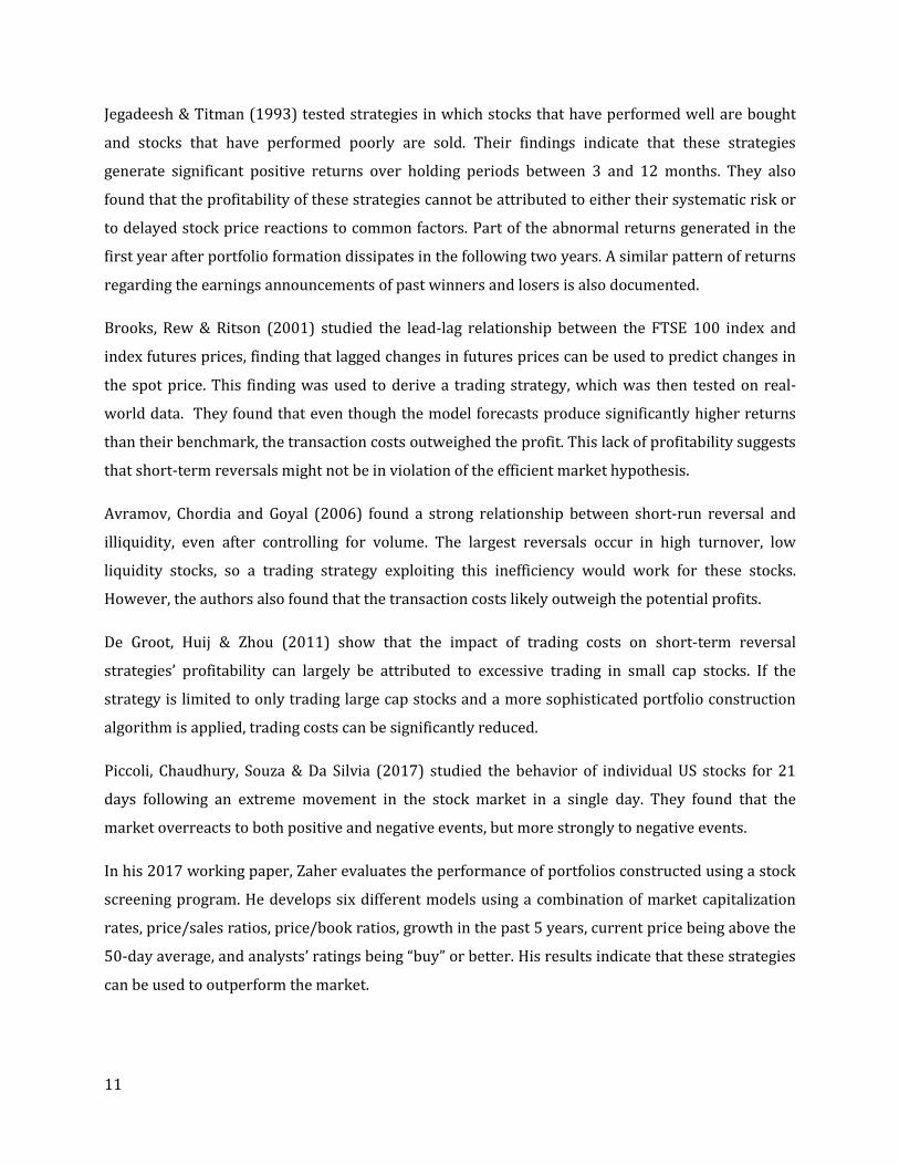
Jegadeesh & Titman (1993) tested strategies in which stocks that have performed well are bought
and stocks that have performed poorly are sold. Their findings indicate that these strategies
generate significant positive returns over holding periods between 3 and 12 months. They also
found that the profitability of these strategies cannot be attributed to either their systematic risk or
to delayed stock price reactions to common factors. Part of the abnormal returns generated in the
first year after portfolio formation dissipates in the following two years. A similar pattern of returns
regarding the earnings announcements of past winners and losers is also documented.
Brooks, Rew & Ritson (2001) studied the lead-lag relationship between the FTSE 100 index and
index futures prices, finding that lagged changes in futures prices can be used to predict changes in
the spot price. This finding was used to derive a trading strategy, which was then tested on real-
world data. They found that even though the model forecasts produce significantly higher returns
than their benchmark, the transaction costs outweighed the profit. This lack of profitability suggests
that short-term reversals might not be in violation of the efficient market hypothesis.
Avramov, Chordia and Goyal (2006) found a strong relationship between short-run reversal and
illiquidity, even after controlling for volume. The largest reversals occur in high turnover, low
liquidity stocks, so a trading strategy exploiting this inefficiency would work for these stocks.
However, the authors also found that the transaction costs likely outweigh the potential profits.
De Groot, Huij & Zhou (2011) show that the impact of trading costs on short-term reversal
strategies’ profitability can largely be attributed to excessive trading in small cap stocks. If the
strategy is limited to only trading large cap stocks and a more sophisticated portfolio construction
algorithm is applied, trading costs can be significantly reduced.
Piccoli, Chaudhury, Souza & Da Silvia (2017) studied the behavior of individual US stocks for 21
days following an extreme movement in the stock market in a single day. They found that the
market overreacts to both positive and negative events, but more strongly to negative events.
In his 2017 working paper, Zaher evaluates the performance of portfolios constructed using a stock
screening program. He develops six different models using a combination of market capitalization
rates, price/sales ratios, price/book ratios, growth in the past 5 years, current price being above the
50-day average, and analysts’ ratings being “buy” or better. His results indicate that these strategies
can be used to outperform the market.

12
In their Bachelor’s thesis from 2017, Funke & Sinjari use monthly data on the stocks in OMXS30
between 2008 and 2017 to test alpha trading. They construct a portfolio where stocks with
historical alphas which are greater than zero are held long and historical alphas which are less than
zero are held short. They conclude that the portfolio constructed by alpha trading increased in value
by 33.45% during a 2-year evaluation period, while OMXS30 increased by 15.29% during the same
period.
4. DATA
In this section, the data used in this thesis is presented. First, the stocks and market index data used
are presented, including a discussion on the stocks missing from the sample. Consequently,
describing the risk free rate concludes this section.
4.1. STOCKS AND MARKET INDEX DATA
In this thesis, estimations are made using individual stocks included in the Dow Jones Industrial
Average and the Standard & Poor’s 500 Index. In the Results section, we also include the Dow Jones
Industrial Average index itself as a benchmark for evaluating the portfolios. Monthly adjusted
closing prices are used. The adjusted close price takes dividends and splits into account, which
contributes to the return the investor receives from holding a given stock. For this reason, using this
measurement when evaluating the profitability of an investment strategy gives us a more correct
estimate of the earnings from holding an individual stock compared to simply using the close price.
The historical data used in this thesis was gathered from Yahoo Finance and spans the period
between January 31, 1997 and January 31, 2018. The data used in this thesis was gathered between
January 29 and July 30, 2018.
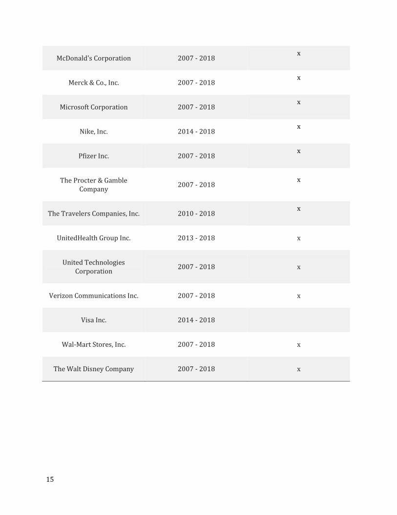
Out of the 30 stocks in the Dow Jones Industrial Average, it proved difficult to get data on up to three
of them for different estimations. In Table 1, the stocks that should have been included are
presented in the left-hand column. The column to the right indicates whether or not the individual
stock is indeed included. Below this table, the stocks excluded from the study are described.

13
Table 1.
Stocks that should have been included in this study
Company stock Years analysed Included
3M Company 2007 - 2018 x
Alcoa Inc. (formerly Aluminum Company
of America) 2007 - 2014 x
Altria Group Incorporated 2007 - 2009 x
American Express Company 2007 - 2018 x
American International Group Inc.
2007 - 2009 x
Apple Inc. 2016 - 2018 x
AT&T Inc. 2007 - 2016 x
Bank of America Corporation 2008 - 2014 x
The Boeing Company 2007 - 2018 x
Caterpillar Inc. 2007 - 2018 x
Chevron Corporation 2007 - 2018 x
Cisco Systems, Inc. 2010 - 2018 x

14
Citigroup Inc. (formerly Travelers Inc.)
2007 - 2010 x
The Coca-Cola Company 2007 - 2018 x
DowDuPont Inc. 2017 - 2018
E.I. DuPont de Nemours & Company Inc.
2007 - 2017 x
Exxon Mobil Corporation 2007 - 2018 x
General Electric Company 2007 - 2018 x
General Motors Corporation 2007 - 2009
The Goldman Sachs Group, Inc. 2014 - 2018 x
Hewlett-Packard Company 2007 - 2014 x
The Home Depot, Inc. 2007 - 2018 x
Honeywell International Inc. 2007 - 2009 x
Intel Corporation 2007 - 2018 x
International Business Machines Corporation
2007 - 2018 x
Johnson & Johnson 2007 - 2018 x
JPMorgan Chase & Co. 2007 - 2018 x
Kraft Foods Inc. 2009 – 2013
15
McDonald's Corporation 2007 - 2018 x
Merck & Co., Inc. 2007 - 2018 x
Microsoft Corporation 2007 - 2018 x
Nike, Inc. 2014 - 2018 x
Pfizer Inc. 2007 - 2018 x
The Procter & Gamble Company
2007 - 2018 x
The Travelers Companies, Inc. 2010 - 2018 x
UnitedHealth Group Inc. 2013 - 2018 x
United Technologies Corporation
2007 - 2018 x
Verizon Communications Inc. 2007 - 2018 x
Visa Inc. 2014 - 2018
Wal-Mart Stores, Inc. 2007 - 2018 x
The Walt Disney Company 2007 - 2018 x

16
4.1.1. STOCKS EXCLUDED FROM THE SAMPLE
Out of the 30 stocks in the Dow Jones Industrial Average, this study uses data on between 27 and 29
stocks for different estimations. It is possible that the excluded stocks have different characteristics
compared to the others in the index. Two stocks had to be excluded because they were not publicly
traded for the entire period; and two had to be excluded due to mergers. The US government
intervened to save General Motors, which is considered an unusual situation. Emails and phone calls
to DuPont, Kraft Foods, and General Motors received no response.
Since DuPont merged with Dow Chemical Company in 2017, their stock is now traded under the
DWDP ticker. As historical data for the DD and DOW tickers is no longer available, the historical data
for the DuPont stock does not range sufficiently far back to be used in this study.
Kraft Foods Inc. was not publicly traded between 1988 and 2001. Between 2001 and 2012, it was
traded under the KFT ticker. On October 1, 2012, Kraft Foods Inc. completed the spin-off of Kraft
Foods Group, Inc. and changed its name to Mondelēz International Inc. Mondelēz traded under the
MDLZ ticker, and the Kraft Foods Group traded under the KRFT ticker.
In 2015, the Kraft Foods Group merged with Heinz and formed The Kraft Heinz Company, which has
since then traded under the KHC ticker. Although data on the development of the MDLZ ticker is
available from 2001 and data on the KHC ticker is available from 2015, data on the KRFT stock
prices is no longer available. For this reason, the Kraft Foods Group stock unfortunately had to be
excluded from this study.
General Motors (GM) was absent from the stock market between June 2009 and November 2010.
Due to the drop in auto sales caused by the financial crisis, the US government took ownership of
General Motors during this period in order to keep the company from going bankrupt.
Visa (V) – Prior to October 3, 2007, Visa comprised four non-stock, separately incorporated
companies that employed 6000 people worldwide: Visa International Service Association (Visa) –
the worldwide parent entity, Visa U.S.A. Inc., Visa Canada Association, and Visa Europe Ltd.
As Visa has not been traded sufficiently long, this stock must be excluded from this study.

17
Although it is likely that these omissions cause exclusion bias, the sign of the net effect of the
exclusion bias is uncertain. Had General Motors been included in the sample before their absence
from the stock market, it would have had a negative effect on the return of the portfolio it would
have been a part of. However, we cannot know which of our portfolios that would have been.
Regarding the stocks excluded due to mergers, it is hard to speculate about how certain portfolios
would have been affected.
4.2. RISK-FREE RATE
In this thesis, US treasury bills with a maturity of 3 months are used as a proxy for the risk-free rate.
This data was gathered from the website of the Federal Reserve Bank of St. Louis and converted
from an annualized discount rate to a simple monthly interest rate (no compounding).
5. EMPIRICAL METHOD
In this thesis, generalized autoregressive conditional heteroscedasticity (GARCH) and threshold-
asymmetric generalized autoregressive conditional heteroscedasticity (TGARCH) models are used
to model variance of the error term. This is done because, although OLS models are poorly equipped
to handle some common properties of financial time series, GARCH-type models are designed to
take these properties into account. By using GARCH-type models, we ensure that our standard
errors are correctly estimated and our test statistics are unbiased, and thus, we avoid making
incorrect inferences caused by violations of the OLS assumptions. This topic is explored in depth in
Section 5.2.
Historical data is used to construct portfolios as if an investment had been made in the end of
January each year, based on the last ten years’ historical alpha values of stocks, and the performance
of these portfolios over the following year is then evaluated. Rebalancing is done once per year.
Monthly adjusted close data is used.
The first portfolios are made as if they had been constructed based on the data from January 31,
1997 up to January 31, 2007, using the composition of the Dow Jones Industrial Average as of
January 31, 2007. The evaluation of each portfolio is then performed as if this portfolio had been

18
bought on January 31, 2007 and held until January 31, 2008. The second portfolio is made as if it
had been constructed based on historical data from January 31, 1998 to January 31, 2008, using the
composition of the Dow Jones Industrial Average as of January 31, 2008. The evaluation is then
performed as if it had been bought on January 31, 2008 and held until January 31, 2009, and so on.
The “day of investment”, January 31, is arbitrarily chosen. Data on the stocks in the Dow Jones
Industrial Average is used to construct the portfolios, and data on the Standard & Poor’s 500 Index
is used as the “market”.
As the natural logarithm of the changes in a time series is close to the change in percentage, so long
as such changes are small, the following approximation for the rate of return is used when working
with the stock prices and market indices:
where is the price of the asset in period t, and is the price of the asset in the previous period.
To estimate alpha, the extended market model introduced by Jensen (1968) is used. It is commonly
represented as follows:
( )
where is the rate of return for each stock i at time t, is the risk-free rate of return at time t, is
the return of the market (here: index), the values are the part of the return that cannot be
explained by the systematic risk, and is the residual for stock i at time t.
As before, the values measure the co-movement of the individual stock i with the market:
Note that the extended market model above is estimated both for the individual stocks to inform the
portfolio formation and for the portfolio evaluation. In the latter case, the index i represents the
individual portfolio rather than the individual stock.
In this thesis, the performance of portfolios containing only stocks to be either held long or sold
short, as well as self-financing portfolios which contain both, are evaluated. Adjusted close prices
are used for both stocks and indices, because the owner of the stock receives dividends, and the
dividend payments will be reflected in stock prices.

19
The financial crisis of 2007-2008 happened during the first few years in the evaluation window, and
this crisis is not a representative period in terms of stock market returns. For this reason, all
analyses are performed both including and excluding the first three years of the study, as a
robustness check.
Short selling is the sale of a security that the seller does not own. To sell a stock short means taking
a theoretically infinite risk (if the stock price goes up), so most professionals who do so will also buy
a call option just above the price level where they made the short sale. Thus, there is a tendency for
stocks that are not optionable to not be sold short as often. Consequently, if this strategy were to be
implemented, fund managers would buy these call options, and this cost would need to be taken
into account when evaluating the practical usefulness this investment strategy.
In order to get a comprehensive picture of the performance of the portfolios, we use three
measures: the alpha value, the Sharpe ratio, and the end value of the portfolio. The alpha value
measures the risk-adjusted return compared to a market index. The Sharpe ratio measures the extra
return received when choosing to accept a higher volatility. The end value measures the actual
return that the investor receives. When we look at these measurements together, we can determine
not only what return we would have received by using this trading strategy but also whether we
would have been fairly compensated for the risk we would have taken – in other words, would we
“beat the market” or simply be compensated for accepting a higher risk?
For ease of comparison, all portfolios’ values at the start of the first evaluation period are
normalized to 100, and for the self-financing portfolios, the starting value for each part is 100, so the
value of the self-financing portfolio is equal to zero.
5.1. PORTFOLIO CREATION
The steps of portfolio creation are:
1. The changes in natural logarithms (“diff-logs”) are calculated for all stocks and the index,
and the risk-free rate is subtracted.
2. We fit the market model (including an alpha term) to the last ten years’ data, which gives us
the estimates of historical alpha values for each stock, as well as the p-values for the
estimated alpha values. This is done using GARCH or TGARCH to model variance. In this
step, two-sided t-tests are used when determining which stocks have estimated alpha values
significantly different from zero.
20
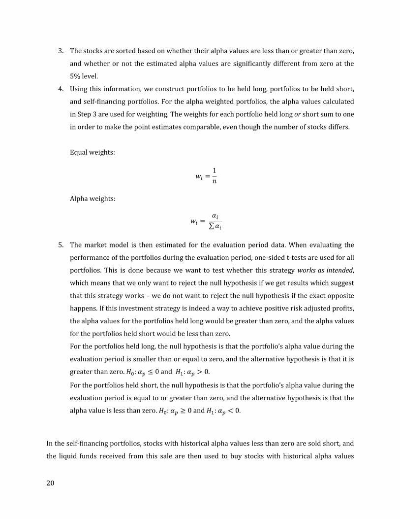
3. The stocks are sorted based on whether their alpha values are less than or greater than zero,
and whether or not the estimated alpha values are significantly different from zero at the
5% level.
4. Using this information, we construct portfolios to be held long, portfolios to be held short,
and self-financing portfolios. For the alpha weighted portfolios, the alpha values calculated
in Step 3 are used for weighting. The weights for each portfolio held long or short sum to one
in order to make the point estimates comparable, even though the number of stocks differs.
Equal weights:
Alpha weights:
∑
5. The market model is then estimated for the evaluation period data. When evaluating the
performance of the portfolios during the evaluation period, one-sided t-tests are used for all
portfolios. This is done because we want to test whether this strategy works as intended,
which means that we only want to reject the null hypothesis if we get results which suggest
that this strategy works – we do not want to reject the null hypothesis if the exact opposite
happens. If this investment strategy is indeed a way to achieve positive risk adjusted profits,
the alpha values for the portfolios held long would be greater than zero, and the alpha values
for the portfolios held short would be less than zero.
For the portfolios held long, the null hypothesis is that the portfolio’s alpha value during the
evaluation period is smaller than or equal to zero, and the alternative hypothesis is that it is
greater than zero. and .
For the portfolios held short, the null hypothesis is that the portfolio’s alpha value during the
evaluation period is equal to or greater than zero, and the alternative hypothesis is that the
alpha value is less than zero. and .
In the self-financing portfolios, stocks with historical alpha values less than zero are sold short, and
the liquid funds received from this sale are then used to buy stocks with historical alpha values

21
greater than zero. Both deals last until the end of the evaluation period. No money is inserted or
withdrawn after the initial investment until the next rebalancing a year later. Here, we assume that
there are no transaction costs, which is an unrealistic but simplifying assumption. Thus, in reality,
the return from this strategy would be smaller than these results suggest, as the transaction costs
would need to be deducted from the profit.
Initially, the plan was to create three portfolios: one held long consisting only of stocks with
significant positive alphas, one held short with only significant negative alphas, and a self-financing
portfolio consisting of equal halves of stocks with significant positive and negative alphas. However,
for most years, there were no stocks with significant negative alphas. Instead, we constructed
portfolios to be held long and sold short, as well as self-financing portfolios, without taking the
significance level of the historical alpha estimate into account; in addition, we constructed portfolios
held long, consisting only of stocks with significant alpha values.
The characteristics of the eight portfolios evaluated in this thesis are summarized in Table 2. Note
that the abbreviation “EW” is used for the equally weighted portfolio, and “AW” is used for the alpha
weighted portfolio. This notation is also used in the Results section to make the tables more orderly
and easier to interpret.

22
Table 2.
Summary of the evaluated portfolios
Portfolio Long Short Only stocks with
significant alpha values
Equal weights Alpha weights
Long, EW x x
Long, AW x x
Long, significant, EW x x x
Long, significant, AW x x x
Short, EW x x
Short, AW x x
Self-financing, EW x x x
Self-financing, AW x x x
The structure of the rolling window analysis is shown in Table 3, where the years shaded with blue
are used for the estimation of the historical alpha values, and the years shaded with red are used for
evaluation.

23
Table 3.
Structure of the rolling window analysis for the entire period
1st iteration 2nd iteration 3rd iteration
1997 1997 1997
1998 1998 1998
1999 1999 1999
2000 2000 2000
2001 2001 2001
2002 2002 2002
2003 2003 2003
2004 2004 2004
2005 2005 2005
2006 2006 2006
2007 2007 2007
2008 2008 2008
2009 2009 2009
2010 2010 2010
5.2. THE GARCH AND TGARCH MODELS
In this thesis, the market model is estimated using generalized autoregressive conditional
heteroscedasticity (GARCH) and threshold-asymmetric GARCH to model the variance of the error
term. For the GARCH and TGARCH models, Student’s t-distribution is used because it has fat tails
(compared to the normal distribution), which is known to be better suited for fitting stock market
returns. The purpose of this section is to show why GARCH-type models are used for financial
analyses and to give an overview of the properties of these models.

24
In order to understand why GARCH models are used rather than the ordinary least squares (OLS)
estimator, we need to look at the assumptions needed for OLS to be the best linear unbiased
estimator. We will see that financial time series often do not fulfill these assumptions.
The assumptions needed for OLS to be the best linear unbiased estimator are:
1. The linear regression model is linear in parameters.
2. The conditional mean of the error term is zero.
3. There is no perfect multicollinearity.
4. There is no homoscedasticity and no autocorrelation.
5. The error terms are normally distributed.
There are multiple issues when using this estimator for financial data. First of all, the normality
assumption is often not fulfilled for this type of data. Instead, financial data tends to have fat tails.
Additionally, heteroscedasticity and autocorrelation may be present. The variance in financial time
series depends not only on the variance during previous periods but also on previous shocks.
Volatility is higher during financial crises and lower during calmer periods.
Had OLS been used while heteroscedasticity is present, we would risk the following issues:
1. Inefficient OLS estimators, which means that the estimators will not have the minimum
variance out of the unbiased estimators.
2. Standard error estimates might be biased, which means that the risk of making a type 1
error would be different from the decided upon significance level. This could lead to making
incorrect inferences.
3. When we regress the individual asset return on the market return, the coefficient of
determination of the market return on the stock return will be underestimated. This means
that systematic risk will be understated, and diversifiable risk will be overstated. As stated
by Fisher & Kamin in their paper, Forecasting systematic risk: Estimates of “raw” beta to take
account of the tendency of beta to change and the heteroscedasticity of residual returns
(1985), these errors in beta estimates lead to an understatement of the systematic risk and
an overstatement of the non-systematic risk. Again, this could lead to making incorrect
inferences.
As we can see, OLS is clearly a poor choice for modeling financial data. Unlike OLS, GARCH models
are designed to model some common properties of financial data: tail heaviness, volatility

25
clustering, leptokurtosis of the marginal distribution, and dependence without autocorrelation. In
addition to these properties, the TGARCH model also captures leverage effects. These properties of
financial data can be described in further detail. A small glossary is provided here:
Tail heaviness means that extreme values are more common than in the normal distribution.
This is true, for example, for the Student’s t-distribution, which is the distribution used for
the GARCH and TGARCH models in this thesis.
Volatility clustering means that if the volatility is high during a certain period, the volatility
tends to remain higher during the subsequent periods, whereas periods with low volatility
are often followed by additional periods of low volatility. (GARCH allows the conditional
variance of the residual to evolve according to an autoregressive-type process, which
captures persistent volatility.)
Leptokurtosis of the marginal distribution is defined as having greater kurtosis than the
normal distribution, which signifies that the distribution is less concentrated to the mean.
Dependence without autocorrelation means that there is serial dependence that does not
take the form of linear correlation.
Leverage effects is the tendency for volatility to increase more following a large price fall,
compared to the period following a price rise of the same magnitude.
In threshold-asymmetric GARCH (TGARCH) models, the specifications use conditional standard
deviations rather than conditional variance. It makes sense to use this type of model in finance, as it
takes into account that positive and negative shocks have different impacts on the volatility of the
financial market. As mentioned in the Theoretical framework section, one assumption made when
using CAPM is that of the risk of asset returns being fully explained by variance of the asset return.
However, variance may not be an adequate measurement of risk in this context, as investors react
differently to positive and negative price shocks. For this reason, TGARCH is used in addition to
GARCH in this thesis.
According to Lim & Sek (2013), asymmetric GARCH models (such as the TGARCH) perform better
during financial crises, whereas symmetric GARCH models perform better during normal (pre- and
post-crisis) periods. Because this thesis deals with data from both types of time periods, results
using both models are presented.
26
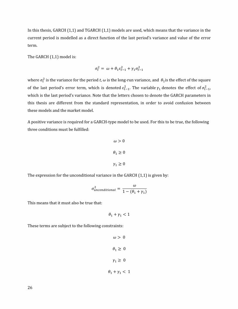
In this thesis, GARCH (1,1) and TGARCH (1,1) models are used, which means that the variance in the
current period is modelled as a direct function of the last period’s variance and value of the error
term.
The GARCH (1,1) model is:
where is the variance for the period t, is the long-run variance, and is the effect of the square
of the last period’s error term, which is denoted . The variable denotes the effect of
,
which is the last period’s variance. Note that the letters chosen to denote the GARCH parameters in
this thesis are different from the standard representation, in order to avoid confusion between
these models and the market model.
A positive variance is required for a GARCH-type model to be used. For this to be true, the following
three conditions must be fulfilled:
The expression for the unconditional variance in the GARCH (1,1) is given by:
This means that it must also be true that:
These terms are subject to the following constraints:

27
The TGARCH (1,1) model can be represented thus:
where is the leverage parameter capturing the asymmetric effects of past shocks. This parameter
is constrained to | | ≤1.

28
6. RESULTS
Below, the results of this study are presented. The order of this section is as follows: first, we go
through the results for the estimations for the whole period using an estimation of the market
model using GARCH for modelling the variance, followed by the results for the estimations for the
whole period using TGARCH for modelling the variance. Next, the results using only the post-crisis
years are presented: first when using GARCH and then when TGARCH is used. The Dow Jones
Industrial Average Index is included in each table for comparison.
Graphs showing the value development for the portfolios are presented with their corresponding
tables. P1 (peach) is the equally weighted portfolio held long; P2 (light blue) is the equally weighted
portfolio held short; P3 (yellow) is the equally weighted portfolio consisting of stocks with
significant alpha values held long; P5 (mustard) is the alpha weighted portfolio held long; P6 (dark
blue) is the alpha weighted portfolio held short; and P7 (brown) is the alpha weighted portfolio
consisting of stocks with significant alpha values held long. The black line represents the Dow Jones
Industrial Average, and the grey line the Standard & Poor’s 500 Index.
The end values for the self-financing portfolios for each analysis are presented together with the
other results of each of the four analyses. At the start of the first evaluation period, each portfolio’s
value is normalized to 100, and for the self-financing portfolios, the starting value for each part is
100, thus the value of each self-financing portfolio is equal to zero.
Unfortunately, portfolios to be held short could not be formed for Years 5 and 11 using GARCH, so
the analyses are done as if no investments were done these years. This means that the evaluation
periods are 9 and 6 years, respectively, instead of 11 and 8 as for the TGARCH analyses.

29
6.1 WHOLE PERIOD, USING GARCH
Graph 1. Value development of the portfolios constructed using GARCH for the whole period

30
In Table 4, we find the results of the evaluation of the portfolios formed using the estimates of the
market model that utilizes GARCH to model the variance. As we can see, three out of four of the
portfolios held long (Long, AW; Long, significant, EW; Long, significant, AW) outperform both of the
indices as well as the portfolios held short in terms of value increase of the portfolio over the
evaluation period. The best performing portfolio in terms of value increase is the alpha weighted
portfolio held long consisting only of stocks with historical alpha values significantly greater than
zero, which increased from a value of 100 to 247 over the course of the evaluation period. Both of
the alpha weighted portfolios perform better than their equally weighted counterparts, at 247
compared to 218 and 176 compared to 122, respectively. The worst performing portfolio in terms of
value increase is the equally weighted portfolio held short, which decreased in value from 100 to
under 34 over the course of the evaluation period.
The portfolios containing only stocks with historical alpha values significantly greater than zero
have the highest mean monthly risk premiums, as well as the highest Sharpe ratios. The Sharpe
ratios of these portfolios are 0.1200 and 0.1296, which is almost four times the Sharpe ratio of the
equally weighted portfolio held short at 0.0391.
However, all alpha values are close to zero and non-significant. This suggests that the difference in
portfolio value development between the portfolios held long and those held short is simply the
result of different risk levels. The same results could have been achieved by buying high-risk stock
and short selling low-risk stock. Thus, there is no evidence here of alpha trading being a successful
investment strategy, but weak form market efficiency appears to hold.

31
Table 4.
Summary of results for 9 years – evaluation of portfolios created using estimates of the market model
using GARCH.
Standard errors for the point estimates of alpha are reported in parentheses below each point estimate.
Significance at the 5% level *, 1% level **, 0.1% level ***
A: evaluated using GARCH
B: evaluated using TGARCH
Portfolio Alpha (A) Alpha (B)
Mean monthly
risk premium
(%)
Sharpe ratio
(monthly)
Portfolio end
value
Dow Jones Industrial
Average
-0.0484
(0.0889)
-0.0518
(0.0205) 0.3047 0.0720 150.2612
Standard & Poor’s
500 Index - - 0.3482 0.0776 157.8581
Long, EW 0.0013
(0.1189)
-0.0774
(0.1213) 0.4326 0.0849 122.1951
Long, AW -0.0982
(0.1731)
-0.1193
(0.1467) 0.5553 0.0999 176.0110
Long, significant, EW 0.2883
(0.3215)
0.0883
(0.4506) 0.6918 0.1200 218.6835
Long, significant, AW 0.1824
(0.2960)
0.0079
(2.1375) 0.6803 0.1296 247.8452
Short, EW 0.1333
(0.2645)
0.1917
(0.0995) 0.2362 0.0391 33.7841
Short, AW -0.0270
(0.5213)
-0.1151
(0.3667) 0.3775 0.0559 87.2686

32
Table 5.
Value of the self-financing portfolios at the end of the evaluation period for the analysis above
End value of the self-financing portfolios
Equally weighted 88.4074
Alpha weighted 88.7424
As we can see in Table 5, this trading strategy would have resulted in a positive profit, and the sizes
are comparable for the equally weighted and alpha weighted portfolios. The size of this profit is
likely large enough to cover the trading costs involved for this investment strategy. Note that this is
not risk-adjusted measure, and a similar result might have been produced by simply buying risky
stocks and selling less risky stocks short.

33
6.2 WHOLE PERIOD, USING TGARCH
Graph 2. Value development of the portfolios constructed using TGARCH for the whole period

34
In Table 6, we can see that the results for the portfolios created using threshold-asymmetric GARCH
resemble those created using GARCH. The best performing portfolio in terms of value increase is the
equally weighted portfolio consisting of stocks with historical alpha values significantly greater than
zero, ending at a value of almost 300. This is a 200% increase compared to the starting value of 100.
The alpha weighted counterpart ended at a value of 282. The worst performing portfolio in terms of
value increase is the equally weighted portfolio held short, which ends at a value of 36, followed by
the alpha weighted portfolio held long, ending at a value of 65.
Here, the alpha weighted portfolio held long has the highest Sharpe ratio at 0.1364, followed by the
alpha weighted portfolio held short with a Sharpe ratio of 0.1124. The portfolio with the lowest
Sharpe ratio is 0.0937 for the equally weighted portfolio held short, followed by the alpha weighted
portfolio consisting only of stocks with historical alpha values significantly greater than zero, with a
Sharpe ratio of 0.0968. Comparing these results to the results using the GARCH model, we can see
that they do not follow the same pattern.
Similar to the portfolios formed using GARCH, the alpha values for the portfolios formed using
TGARCH are all close to zero. Thus, there is no proof of this investment strategy being successful.

35
Table 6.
Summary of results for 11 years – evaluation of portfolios created using estimates of the market model
using TGARCH.
Standard errors for the point estimates of alpha are reported in parentheses below each point estimate.
Significance at the 5% level *, 1% level **, 0.1% level ***
A: evaluated using GARCH
B: evaluated using TGARCH
Portfolio Alpha (A) Alpha (B)
Mean monthly
risk premium
(%)
Sharpe ratio
(monthly)
Portfolio end
value
Dow Jones Industrial
Average
0.0443
(0.0834)
0.0426
(0.2499) 0.4953 0.1214 207.1782
Standard & Poor’s
500 Index - - 0.4546 0.1052 196.3379
Long, EW 0.0076
(0.0920)
-0.0623
(0.0820) 0.5043 0.1108 152.1426
Long, AW 0.1832
(0.1269)
0.1405*
(0.0388) 0.6435 0.1364 65.8701
Long, significant, EW 0.0467
(0.3549)
0.0734
(0.3260) 0.6056 0.1043 299.5673
Long, significant, AW 0.0514
(0.4755)
0.1009
(0.5178) 0.5563 0.0968 282.4570
Short, EW 0.3696
(0.2615)
0.2288
(0.2459) 0.5903 0.0937 36.0056
Short, AW 0.3870
(0.3709)
0.3717
(0.4328) 0.7953 0.1124 69.8764

36
Table 7.
Value of the self-financing portfolios at the end of the evaluation period for the analysis above
End value of the self-financing portfolios
Equally weighted 116.137
Alpha weighted -4.0063
In Table 7, we can see that the equally weighted self-financing portfolio would have made a
relatively large profit, whereas the alpha weighted portfolio would have resulted in a small loss at
the end of the period. Again, note that this is not a risk-adjusted measure, and a similar result for the
equally weighted portfolio could have been achieved by buying high-risk and short selling low-risk
stocks.
37
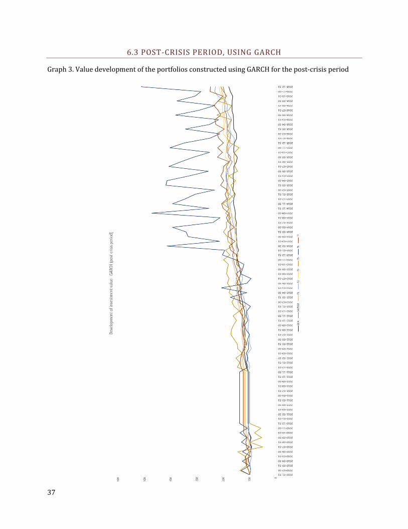
6.3 POST-CRISIS PERIOD, USING GARCH
Graph 3. Value development of the portfolios constructed using GARCH for the post-crisis period

38
Table 8.
Summary of results for 6 years, using only the period after the financial crisis of 2007-2008. Evaluation
of portfolios created using estimates of the market model using GARCH.
Standard errors for the point estimates of alpha are reported in parentheses below each point estimate.
Significance at the 5% level *, 1% level **, 0.1% level ***
A: evaluated using GARCH
B: evaluated using TGARCH
Portfolio Alpha (A) Alpha (B)
Mean monthly
risk premium
(%)
Sharpe ratio
(monthly)
Portfolio end
value
Dow Jones Industrial
Average
-0.1132
(0.0840)
-0.1181
(0.0873) 0.8498 0.2532 179.5857
Standard & Poor’s
500 Index - - 1.0067 0.2945 200.7803
Long, EW 0.0202
(0.1546)
0.0101
(0.1308) 0.9965 0.2970 209.1085
Long, AW -0.1583
(0.1480)
-0.1583
(0.1481) 1.0661 0.2780 210.1931
Long, significant, EW -0.0366
(0.2732)
-0.0366
(0.2732) 1.0164 0.2486 216.2216
Long, significant, AW -0.1004
(0.2806)
-0.0446
(0.2832) 1.0759 0.2775 249.1100
Short, EW 0.1358
(0.2539)
0.0853
(0.2879) 1.1962 0.2829 229.9109
Short, AW 0.1821
(0.3420)
-0.0113
(0.4386) 0.9932 0.2359 512.6575

39
In Table 8, we can see that the results of the first analysis change when we exclude the period up
until the end of the financial crisis of 2007-2008 from the evaluation period. The estimates of the
market model, which the portfolios are based on, use GARCH to model the variance.
As we can see in the table above, the best performing portfolio in terms of value increase is the
alpha weighted portfolio held short, with an end value of almost 513. The portfolio with the second
highest end value is the alpha weighted portfolio consisting only of stocks with historically
significant alpha values, with an end value of 249. The worst performing portfolio in terms of value
increase is the equally weighted portfolio held long, ending at 209, followed by the alpha weighted
portfolio held long, ending at 210.
It is worth noting that although it might seem strange that all portfolios outperform the Dow Jones
Industrial Average Index, such could be the case either due to the excluded stocks (described in
Section 4.1.1.) or simply due to different methods of weighting. In this thesis, alpha weighting and
naïve weighting are used, but the Dow Jones Industrial Average is price-weighted. Thus, if relatively
cheaper stocks have had better developments compared to more expensive stocks, this would yield
results such as these.
The equally weighted portfolio held long has the highest Sharpe ratio at 0.2970, followed by the
equally weighted portfolio held short at 0.2829. The alpha weighted portfolio held short has the
lowest Sharpe ratio at 0.2359, followed by the equally weighted portfolio consisting only of stocks
with historical alpha values significantly greater than zero, with a Sharpe value of 0.2486.
Again, all the estimated alpha values are non-significant, and weak-form market efficiency appears
to hold.
Table 9.
Value of the self-financing portfolios at the end of the evaluation period for the analysis above
End value of the self-financing portfolios
Equally weighted -20.8024
Alpha weighted -302.4644

40
When comparing the results in Table 9, we see that unlike the results for the entire period, the
results for the post-crisis period are that the self-financing portfolios result in a small loss for the
equally weighted portfolio and a great loss for the alpha weighted portfolio. Thus, we can conclude
that this does not appear to be a successful trading strategy.

41
6.4 POST-CRISIS PERIOD, USING TGARCH
Graph 4. Value development of the portfolios constructed using TGARCH for the post-crisis period

42
Table 10.
Summary of results for 8 years, using only the period after the financial crisis of 2007-2008. Evaluation
of portfolios created using estimates of the market model using TGARCH.
Standard errors for the point estimates of alpha are reported in parentheses below each point estimate.
Significance at the 5% level *, 1% level **, 0.1% level ***
A: evaluated using GARCH
B: evaluated using TGARCH
Portfolio Alpha (A) Alpha (B)
Mean monthly
risk premium
(%)
Sharpe ratio
(monthly)
Portfolio end
value
Dow Jones Industrial
Average
0.0139
(0.0865)
0.0369*
(0.0210) 0.9756 0.2936 245.5390
Standard & Poor’s
500 Index - - 0.9884 0.2884
248.96963
Long, EW -0.0856
(0.1644)
-0.1144
(0.1138) 0.9191 0.2691 242.1888
Long, AW 0.0541
(0.1123)
-0.1103
(0.2543) 0.9483 0.2620 220.2114
Long, significant, EW -0.2628
(0.3041)
-0.2220
(0.3334) 0.8720 0.2066 305.7967
Long, significant, AW -0.3099
(0.2536)
-0.2932
(0.2626) 0.7616 0.1634 358.7534
Short, EW 0.7013
(0.3041)
0.5981
(0.3066) 1.5020 0.3405 198.6051
Short, AW 0.8720
(0.3069)
0.7591
(1.4299) 1.8352 0.3692 209.0518
43
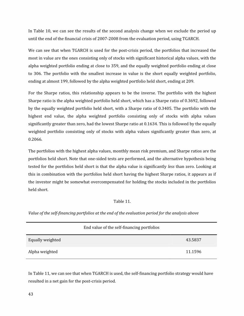
In Table 10, we can see the results of the second analysis change when we exclude the period up
until the end of the financial crisis of 2007-2008 from the evaluation period, using TGARCH.
We can see that when TGARCH is used for the post-crisis period, the portfolios that increased the
most in value are the ones consisting only of stocks with significant historical alpha values, with the
alpha weighted portfolio ending at close to 359, and the equally weighted portfolio ending at close
to 306. The portfolio with the smallest increase in value is the short equally weighted portfolio,
ending at almost 199, followed by the alpha weighted portfolio held short, ending at 209.
For the Sharpe ratios, this relationship appears to be the inverse. The portfolio with the highest
Sharpe ratio is the alpha weighted portfolio held short, which has a Sharpe ratio of 0.3692, followed
by the equally weighted portfolio held short, with a Sharpe ratio of 0.3405. The portfolio with the
highest end value, the alpha weighted portfolio consisting only of stocks with alpha values
significantly greater than zero, had the lowest Sharpe ratio at 0.1634. This is followed by the equally
weighted portfolio consisting only of stocks with alpha values significantly greater than zero, at
0.2066.
The portfolios with the highest alpha values, monthly mean risk premium, and Sharpe ratios are the
portfolios held short. Note that one-sided tests are performed, and the alternative hypothesis being
tested for the portfolios held short is that the alpha value is significantly less than zero. Looking at
this in combination with the portfolios held short having the highest Sharpe ratios, it appears as if
the investor might be somewhat overcompensated for holding the stocks included in the portfolios
held short.
Table 11.
Value of the self-financing portfolios at the end of the evaluation period for the analysis above
End value of the self-financing portfolios
Equally weighted 43.5837
Alpha weighted 11.1596
In Table 11, we can see that when TGARCH is used, the self-financing portfolio strategy would have
resulted in a net gain for the post-crisis period.

44
Looking at all these results together, we must conclude that there is no evidence in this study to
suggest that alpha trading would work consistently. We see that the portfolios consisting of stocks
with historical alpha values significantly greater than zero have an end date value larger than both
of the market indices in every analysis, but they also have non-significant alpha values. This means
that although they increase in value, they do not beat the market. The investor is simply being
compensated for a higher risk.
Although the portfolios consisting of stocks with significant historical alpha values have the greatest
increase in value, they do not have consistently positive alpha values during the evaluation period,
and they have equal or lower Sharpe ratios than the other portfolios. This suggests a relationship
between large historical alpha values and both a higher future volatility and value increase.
For the post-crisis period, the portfolios held short have the highest alpha values. Thus, it appears as
if there might be a relationship between poor historical performance and future positive risk-
adjusted profit. This is in line with the positive results of some of the studies of reversal portfolio
strategies mentioned in the Previous studies section.
45
7. DISCUSSION
The purpose of this thesis was to determine if alpha trading would have worked, had it been used in
the US stock market during the past eleven years. This was done using the stocks included in the
Dow Jones Industrial Average between 1997 and 2018. The performance of portfolios made up of
stocks with historical alpha values greater than zero, portfolios with historical alpha values less
than zero, and self-financing portfolios containing both were studied. The performance of equal
weighting and alpha weighting were compared. These analyses were done using both the whole
period as well as the post-crisis period (after 2007-2008). The data was fitted to the GARCH and
threshold-asymmetric GARCH models, because they are known to be well suited for working with
financial data.
From these results, we can conclude that this trading strategy does not work consistently.
When the financial crisis period is included in the sample, the portfolios with historical alpha values
greater than zero increase more in value than the portfolios with historical alpha values less than
zero. However, all portfolios have alpha values close to zero, so the higher payoff is associated with
a higher risk level.
For the post-crisis period, there is a tendency for the portfolios containing stocks with historical
negative alpha values to outperform the portfolios containing stocks with historical positive alpha
values in terms of the size of the alpha value. We can also conclude that the portfolios consisting of
stocks with alpha values significantly greater than zero increase in value more than the portfolios
consisting of all stocks with alpha values greater than zero. However, this is not the result of a larger
risk-adjusted profit but rather appears to be a relationship between stocks with historical alpha
values significantly greater than zero and high future risk levels, and thus, the investor is simply
being compensated for this risk.
Between one and three (out of 30) stocks are missing in each analysis of the stocks in the Dow Jones
Industrial Average, and it is likely that the stocks for which data for the whole period cannot be
obtained differ systematically from those for which data could be obtained. This means that these
results may not be generalizable for the US stock market as a whole.

46
Some suggestions for future research are: studying how this trading strategy would work for high-
frequency data, such as daily data or intraday data; looking into whether or not these models can be
improved by allowing for cyclicity; testing the effects of rebalancing at different intervals, e.g. every
3 or 6 months instead of every 12 months as in this thesis; or using different stocks. As the US stock
market is more closely watched than other markets, and the Dow Jones Industrial Average contains
some of the most closely watched stocks on the US stock market, it would be interesting to see to
what extent these results are generalizable to other markets.

47
REFERENCES
ARTICLES
Avramov, Doron and Chordia, Tarun and Goyal, Amit “Liquidity and Autocorrelations in Individual
Stock Returns” (2006)
The Review of Financial Studies. 19(4), pp. 1241–1277
De Bondt, Werner F. M. and Thaler, Richard “Does the Stock Market Overreact?” (1985)
The Journal of Finance. 40 (3), pp. 793-805
Brooks, Chris and Rew, Alistair G and Ritson, Stuart “A trading strategy based on the lead–lag
relationship between the spot index and futures contract for the FTSE 100” (2001)
International Journal of Forecasting. 17(1), pp. 31-44
Fama, Eugene F. “Efficient Capital Markets: Review of Theory and Empirical Work” (1970)
The Journal of Finance. 25 (2), pp. 383-417.
Fisher, Lawrence and Kamin, Jules H. “Forecasting systematic risk: Estimates of „raw” beta to take
account of the tendency of beta to change and the heteroscedasticity of residual returns” (1985)
Journal of Financial and Quantitative Analysis, 20 (2), p. 127–149.
French, Jordan “Back to the Future Betas: Empirical Asset Pricing of US and Southeast Asian Markets”
(2016)
International Journal of Financial Studies. 4 (3): 15
Funke, Linnéa and Sinjari, Ronny “Bli en Alfa på den svenska aktiemarknaden - En empirisk studie om
portföljvalsstrategi baserat på alpha trading” (2017)

48
De Groot, Wilma and Huij, Joop and Zhou, Weili “Another Look at Trading Costs and Short-Term
Reversal Profits” (2011)
Jegadeesh, Narasimhan and Titman, Sheridan “Returns to Buying Winners and Selling Losers:
Implications for Stock Market Efficiency” (1993)
The Journal of Finance, 48 (1)., pp. 65-91.
Jensen, Michael "The Performance Of Mutual Funds In The Period 1945–1964" (1968)
The Journal Of Finance. 23 (2) , pp. 389-416.
Kaul, Gautam and Nimalendran, Mahendrarajah “Price reversals: Bid-ask error or market
overreaction?” (1990)
Journal of Financial Economics. 28 (1), pp 67-93.
Lehmann, Bruce N.”Fads, Martingales, and Market Efficiency” (1990)
The Quarterly Journal of Economics. 105 (1), pp. 1-28
Lim, Ching Mun and Sek, Siok Kun “Comparing the performances of GARCH-type models in capturing
the stock market volatility in Malaysia” (2013)
International Conference on Applied Economics
Lintner, John “The Valuation of Risk Assets and the Selection of Risky Investments in Stock Portfolios
and Capital Budgets” (1965)
The Review of Economics and Statistics 47 (1), pp. 13-37
Markowitz, Harry "Portfolio Selection" (1952)
The Journal of Finance. 7(1): pp. 77–91.

49
Mossin, Jan “Equilibrium in a Capital Asset Market” (1966)
Econometrica 34 (4), pp. 768-783
Piccoli, Pedro and Chaudhury, Mo and Souza, Alceu; da Silva, Wesley Vieira “Stock overreaction to
extreme market events” (2017)
North American Journal of Economics and Finance. 41: pp. 97 – 111.
Roll, Richard "A critique of the asset pricing theory's tests Part I: On past and potential testability of
the theory" (1977)
Journal of Financial Economics, 4 (2): pp. 129–176
Rosenberg, Barr and Reid, Kenneth and Lanstein, Ronald “Persuasive evidence of market inefficiency”
(1985)
The Journal of Portfolio Management Spring 1985, 11 (3) pp. 9-16
Sharpe, William F. “Capital Asset Prices: A Theory of Market Equilibrium under Conditions of Risk”
(1964)
The Journal of Finance. 19 (3), pp. 425-442
Treynor, Jack “Market Value, Time, and Risk” (1961)
Unpublished manuscript.
Zaher, Taher “The Value of Active Investment Strategies” (2017)
NFI Working Papers 2017-WP-02, Indiana State University, Scott College of Business, Networks
Financial Institute.
50
WEBPAGES
Board of Governors of the Federal Reserve System (US), 3-Month Treasury Bill: Secondary Market
Rate [TB3MS], retrieved from FRED, Federal Reserve Bank of St. Louis
Retrieved from https://fred.stlouisfed.org/series/TB3MS (Last accessed 2018-02-21)
Investopedia – CAPM
Retrieved from https://www.investopedia.com/terms/c/capm.asp (Last accessed 2018-03-06)
Investopedia – Short selling
Retrieved from https://www.investopedia.com/terms/s/shortselling.asp (Last accessed 2018-03-
06)
Yahoo Finance
Retrieved from https://finance.yahoo.com/ (Last accessed 2018-03-06)