Evaluating the Performance of Dynamic and Tobit …economics.soc.uoc.gr/macro/docs/Year/2016/papers/paper_3_183.pdf · Evaluating the Performance of Dynamic and Tobit Models in Predicting

Evaluating the Performance of Dynamic and Tobit Models inPredicting Credit Default

Arjana Brezigar-Masten

University of Primorska, Faculty of Mathematics, Natural Sciences and Information Technology and Institute

of Macroeconomic Analysis and Development

Igor Masten1

University of Ljubljana, Faculty of Economics, and Bank of Slovenia

Matjaz Volk1

Bank of Slovenia

Abstract

In this paper we analyse the performance of various credit default models in predicting non-performing borrowers and transitions to default. In addition to conventional binary classifiers,which are typically used in practice, we evaluate the performance of two novel methodologies -dynamic and tobit credit risk models. Moreover, we introduce an approach for modelling creditdefault on quarterly frequency using mixed frequency data. We show that tobit model, whereoverdue in loan repayment is modelled explicitly, outperforms all the other models. The choicebetween dynamic and static version of the model depends whether one is interested in predictingstate of non-performing borrowers or new defaulters. For the former, the persistence is of a keyimportance and therefore the dynamic model is the advantageous modelling methodology. Forpredicting new defaulters, however, static tobit model is shown to outperform all other modelsin terms of true positive rate by a large margin. Our results show that the prevailing credit riskmethodologies can be significantly improved by including the dynamics and choosing the tobitfunctional form. This is especially pronounced for conventional default probability model thatis typically used by banks and regulators and is shown to have very low classification accuracy.A number of robustness checks confirm the validity of the results.

JEL-Codes: C24, C25, G21, G32, G33

Keywords: credit default, probability of default, dynamic model, tobit, mixed-frequencydata

Email addresses: [email protected] (Arjana Brezigar-Masten), [email protected] (IgorMasten), [email protected] (Matjaz Volk)

1The views expressed in this paper are solely the responsibility of the authors and should not be interpretedas reflecting the views of the Bank of Slovenia.

1. Introduction

Credit default models are extensively used by banks and regulators. IRB regulation requiresfrom banks to provide their own estimates of probability of default, which is one of the key pa-rameters that determines capital requirements (BCBS, 2001, 2006). Identifying non-performingborrowers also enables banks and regulators to project expected losses and to assess potentialcapital needs to cover these losses. In addition, default probability models can also be used forstress testing purposes to simulate the effect of different scenarios.

In this paper we propose and test the performance of two novel methodologies for modellingcredit risk. Credit default is typically modelled using discrete choice methodology as was firstproposed by Altman (1968). The binary dependent variable is usually defined following BCBS(2006) default definition, which is based on number of days past due. The default event occurswhen borrower is more than 90 days overdue. By transforming an overdue into a dichotomousvariable, a lot of potentially useful information is lost. In addition, overdue is already a riskmeasure and therefore it seems reasonable to model it directly, without any transformations.Since it is censored at value zero, we apply tobit modelling approach. Our first set of tests isaimed to evaluate and compare the performance of classical binary probit model versus tobitmodel.

Credit default indicators show a lot of persistence. Once a borrower defaults (becomes morethan 90 days overdue), it is not very likely that he will become performing again. Moreover,an overdue, once being positive, is expected to increase in time. Estimating default probabilitymodel, which includes autoregressive dynamics can thus significantly improve predicting per-formance. Our second proposed novelty is thus to estimate dynamic probit and dynamic tobitmodel using Wooldridge (2005) methodology and compare their performance with static versionof the models.

We evaluate the performance of the models by looking at their ability to discriminate betweenperforming and non-performing borrowers. Conventional default probability models, however,usually follow the discrete time hazard rate modelling approach, which gives the probabilitythat borrower defaults in current period under the condition the default event did not occurbefore (see for instance Bonfim, 2009 and Carling et al., 2007). As described by Hamerle et al.(2003) this in an underlying methodology of IRB regulation. We therefore also estimate classicaldefault probability model, where only transitions to default are taken into account, and compareits performance in predicting new defaulters with other proposed models. Our goal is not to findthe best performing model specification, but rather to use the same explanatory variables in allthe estimates and see how different functional form (probit vs. tobit) and different informationset (static vs. dynamic) affects the performance in explaining state of default and transition todefault. The performance of the models is evaluated using the data of Slovenian non-financialfirms.

We find that tobit modelling methodology outperforms all other models. In predicting non-performing borrowers, where persistence is of a key importance, dynamic tobit correctly identifiesmore than 70% of defaulters and issues less than 1% of false alarms. High performance - 66% truepositive rate - is also achieved by dynamic probit model, which outperforms the static versionby more than 30 percentage points. An important advantage of tobit model, however, is that itsprediction is number of days past due, which enables to form different classes of overdue. Onecan for instance predict defaulters using any overdue threshold, not only 90 days as is standardin binary models. We show that dynamic tobit has high classification accuracy across differentclasses of overdue, from 30 to 360 days. For predicting new defaulters, however, we find that thestatic tobit model is the advantageous modelling approach. It correctly identifies more than 50%of new defaulters and outperforms all the other models by a large margin. It also issues more

2

false alarms comparing to other methodologies, but given the gain in identifying defaulters, thisloss is relatively small and acceptable. This is especially true if one is more concerned in missingdefaulters (type I error) than issuing false alarms (type II error), like is typically assumed in earlywarning literature (see Alessi & Detken, 2011 and Sarlin, 2013). Even though classical binarydefault probability model is estimated explicitly on transitions to default, it is able to correctlyidentify only 5% of new defaulters. Three sets of robustness checks confirm the validity of ourresults.

Our paper is related to a recent study performed by Jones et al. (2015). They test the perfor-mance of various binary classifiers in predicting credit rating changes. In addition to conventionaltechniques such as probit/logit, they also evaluate the performance of more advanced approacheslike non-linear classifiers, neural networks, support vector machines and others. They find thatnewer classifiers significantly outperform all other modelling approaches. Although the goal ofour paper is very similar, it provides two new pieces of evidence. First, we show the performanceof the models can be significantly improved if, instead of conventional binary model, tobit mod-elling methodology is applied. Second, we provide evidence that the dynamic specification ofthe model significantly improves the performance in predicting non-performing borrowers. Toour knowledge both, tobit and dynamic methodologies, have not yet been applied to credit riskmodelling. Moreover, we propose an approach for modelling credit default on quarterly frequencyusing mixed frequency data. This enables to monitor the changes in credit portfolio on higherfrequency and also more accurately since the information set is updated each quarter.

The findings of this paper have important implications for banks and banking regulation. Weshow that the conventional default probability model that is typically used by IRB banks achievesvery low classification accuracy. This poses a question whether this modelling approach, whichat the end determines banks capitalisation, is an appropriate methodology. A simple upgradeof the model with dummies indicating overdue in previous period significantly improves theclassification accuracy. The performance can be further improved by using the tobit modellingapproach. Although the prediction of the tobit model, which is days past due, can not be directlyused in IRB formula for capital requirements, this approach is far more accurate in identifyingnew defaulters, and therefore it seems reasonable to use it in practice.

The rest of the paper is structured as follows. Section 2 provides descriptive analysis ofthe dynamics of different credit risk measures. In Section 3 we present the methodology forestimating and evaluating different credit default models. Estimation and evaluation resultsare presented in Section 4. Section 5 presents three sets of robustness checks, while Section 6concludes the paper and discusses implications.

2. The dynamics of credit default measures

The key data source for our analysis is Credit register of Bank of Slovenia, which is excep-tionally rich database with many information that are not publicly available. The variable weare most interested in is overdue in loan repayment, which signals financial problems of firmsand is also a key credit risk measure under Basel regulation (see BCBS, 2006). It is first avail-able in 2007q4, which limits our analysis to 29 quarterly cross sections from 2007q4 to 2014q4.Restricting the analysis to non-financial firms, which were during the crisis shown to be the mostproblematic segment, results in large sample of more than 1 million observations represented bya triple firm-bank-time.

Figure 1 shows the evolution of loans broken down to different classes of days of overdue inloan repayment. It can be seen that after the start of the crisis in 2008q4, the share of non-performing loans started rising rapidly and reached very high levels. The share of loans withmore than 90 days overdue, which is a standard measure of non-performing loans (BCBS, 2006),

3

rose by more than 25 percentage points until the third quarter of 2013. In 2013q4 it droppedby 8 percentage points, which is the result of transfer of bad loans from two largest banksto Bank Assets Management Company (BAMC). It should thus not be understand as naturalimprovement of banks’ credit portfolio, but rather as an institutional measure that reduced thepressing burden of non-performing loans. Second tranche of transfer was carried out at the endof 2014. Contrary to non-performing loans, the share of loans with 0 days overdue droppedconsiderably in times of financial stress.

Figure 1: Share of loans across different classes of overdue (in %)

Source: Bank of Slovenia, own calculations.

Other classes between 0 and 90 days overdue represent only a small share of total loans, sincethese are in many cases only transition classes to higher days past due. The only exception isclass between 0 and 30 days, which represents around 3 to 10 percentage share of total loans.There are many borrowers who occasionally have small delays in loan repayment, but whoseoverdue does not necessarily increase from one period to another.

Figure 1 reveals that overdue is highly autoregressive process. It can be best seen by increasingshare of loans with overdue above 360 days. Once an overdue bridges a certain threshold, it isexpected to increase in time and reach higher number of days past due. Since these borrowersare financially very weak and are not able to pay back their debt to banks, they are sooner orlatter expected to bankrupt. In 83% of cases when an overdue changed between two consecutivequarters, this change was positive. This finding is partly the result of the fact that overdue iscensored at zero, which means that by the nature of the variable the increases could be muchmore frequent. However, even when we look only at the cases when overdue> 0, we get a similarresult: 80% increases and only 20% decreases. This dynamic is, however, very heterogeneousacross different classes of overdue. As can be seen in Table 1, an overdue is more likely todecrease between two consecutive quarters when it is lower than 30 days. This is the result ofalready mentioned occasional delayers who are in majority of cases able to repay the debt and

4

their overdue thus typically returns to zero in the next quarter. In other classes positive dynamicprevails and the higher is the overdue, more likely it is, that it will further increase. This is tobe expected, since once an overdue exceeds a certain threshold, it is not very likely that a firmwill ever be able to repay the debt.

Table 1: Share of increases and decreases of overdue over different classes, in %

Overdue One quarter horizon One year horizonclass % of increases % of decreases % of increases % of decreases

0 days 4.4 - 8.7 -0-5 days 27.4 57.7 34.4 56.55-10 days 36.2 58.7 43.3 52.910-20 days 41.0 52.9 48.3 47.520-30 days 46.6 47.6 50.1 45.030-60 days 53.4 43.5 57.5 40.260-90 days 62.9 35.5 66.0 32.690-180 days 75.6 23.5 74.1 25.2180-360 days 88.8 10.9 84.3 15.4>360 days 95.3 4.6 91.5 8.4

Source: Bank of Slovenia, own calculations.Note: The table reports the percentage of increases and decrease of overdue over differentclasses of overdue and two horizons.

Looking at changes in one year period in Table 1 reveals similar dynamic, but decreasesprevail only until overdue is below 10 days. In addition, with exception of last three classes,the increases of overdue are more frequent on yearly basis than quarterly. This means that alsoborrowers with fewer days past due can be more problematic on a long run. Although they werein majority of cases able to repay their debt on a short run, this signals that they might not beable to do so on a long run. Overall, Table 1 clearly reveals that overdue has strong positiveautoregressive component, especially when it is higher than 30 days.

Default rate and its projection, probability of default, is typically of a main interest in banks,since it is one of the key factors that determines projected expected losses and capital require-ments for IRB banks. In addition, PD is also an important factor in loan approval and pricing.Table 2 shows the default rate over different classes of overdue. It is calculated as a share ofborrowers that had been performing in time t − 1 and became more than 90 days overdue intime t. As expected, the share of transitions to non-performing status is higher, the higher wasthe overdue in previous period and it further increases when calculated on one year horizon.Lower levels of overdue can thus be used as an early warning signal for potential defaulters infuture periods. Classical PD model, where the transition to default is typically explained withborrower-specific factors, is unable to fully capture this information. It only captures some partof it when problems in loan repayment are reflected also in firm financial ratios. These, however,are usually available only once a year, which disable updating the estimated probabilities ofdefault on the same frequency as overdue is refreshed.

Our analysis thus far reveals three potential upgrades of current prevailing credit risk mod-elling techniques. First, overdue by itself is already a risk measure and thus it seems naturalto model it directly. A lot of useful and valuable information is lost, when it is transformed todichotomous variable and estimated with discrete choice model. An overdue, even if it is low,signals financial problems of a firm and it is thus important to monitor the whole spectrum ofdelays in loan repayment. Second, autoregressive component seems to be an important factorin modelling credit risk. As shown, an overdue is expected to increase in time, whereas default

5

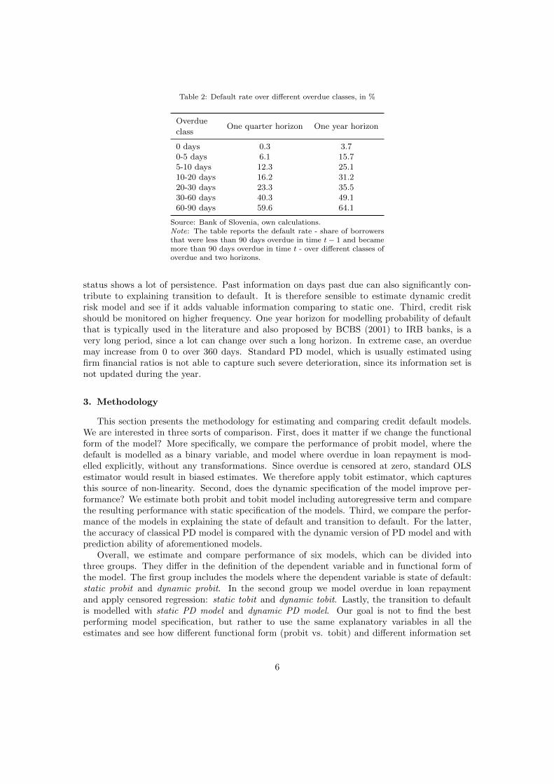
Table 2: Default rate over different overdue classes, in %

Overdue

classOne quarter horizon One year horizon

0 days 0.3 3.70-5 days 6.1 15.75-10 days 12.3 25.110-20 days 16.2 31.220-30 days 23.3 35.530-60 days 40.3 49.160-90 days 59.6 64.1

Source: Bank of Slovenia, own calculations.Note: The table reports the default rate - share of borrowersthat were less than 90 days overdue in time t− 1 and becamemore than 90 days overdue in time t - over different classes ofoverdue and two horizons.

status shows a lot of persistence. Past information on days past due can also significantly con-tribute to explaining transition to default. It is therefore sensible to estimate dynamic creditrisk model and see if it adds valuable information comparing to static one. Third, credit riskshould be monitored on higher frequency. One year horizon for modelling probability of defaultthat is typically used in the literature and also proposed by BCBS (2001) to IRB banks, is avery long period, since a lot can change over such a long horizon. In extreme case, an overduemay increase from 0 to over 360 days. Standard PD model, which is usually estimated usingfirm financial ratios is not able to capture such severe deterioration, since its information set isnot updated during the year.

3. Methodology

This section presents the methodology for estimating and comparing credit default models.We are interested in three sorts of comparison. First, does it matter if we change the functionalform of the model? More specifically, we compare the performance of probit model, where thedefault is modelled as a binary variable, and model where overdue in loan repayment is mod-elled explicitly, without any transformations. Since overdue is censored at zero, standard OLSestimator would result in biased estimates. We therefore apply tobit estimator, which capturesthis source of non-linearity. Second, does the dynamic specification of the model improve per-formance? We estimate both probit and tobit model including autoregressive term and comparethe resulting performance with static specification of the models. Third, we compare the perfor-mance of the models in explaining the state of default and transition to default. For the latter,the accuracy of classical PD model is compared with the dynamic version of PD model and withprediction ability of aforementioned models.

Overall, we estimate and compare performance of six models, which can be divided intothree groups. They differ in the definition of the dependent variable and in functional form ofthe model. The first group includes the models where the dependent variable is state of default:static probit and dynamic probit. In the second group we model overdue in loan repaymentand apply censored regression: static tobit and dynamic tobit. Lastly, the transition to defaultis modelled with static PD model and dynamic PD model. Our goal is not to find the bestperforming model specification, but rather to use the same explanatory variables in all theestimates and see how different functional form (probit vs. tobit) and different information set

6

(static vs. dynamic) affects the performance in explaining state of default and transition todefault.

To our knowledge this is the first attempt to model credit default in a dynamic setting.There are some analysis, like for instance Costeiu and Neagu (2013), where past information areincluded in the model, but not explicitly as lagged dependent variable. Hence, we first presentsome theory and solutions on how to estimate dynamic non-linear panel data models. Next, wepresent the specification of all the models and describe how we evaluate their performance.

3.1. Dynamic non-linear panel data models

The key issue in estimating dynamic panel data models is the initial conditions problem, whichis the result of correlation between unobserved heterogeneity and past values of the dependentvariable. In linear models this problem can be easily solved with appropriate transformation,like first differencing, which eliminates the unobserved effects. Although the transformed errorterm is correlated with transformed lagged dependent variable, instrumental variables can beused to achieve a consistent estimator. Anderson and Hsiao (1982) propose using yit−2 as aninstrument in first-differenced equation. Arellano and Bond (1991) upgrade this approach byusing a GMM-type of model with all possible instruments in each time period, whereas Blundelland Bond (1998) propose a system estimator, where also level equation with instruments indifferences is estimated.

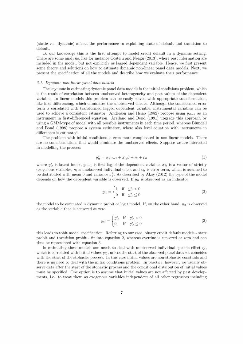
The problem with initial conditions is even more complicated in non-linear models. Thereare no transformations that would eliminate the unobserved effects. Suppose we are interestedin modelling the process:

y∗it = αyit−1 + x′itβ + ηi + εit (1)

where y∗it is latent index, yit−1 is first lag of the dependent variable, xit is a vector of strictlyexogenous variables, ηi is unobserved individual effect and εit is error term, which is assumed tobe distributed with mean 0 and variance σ2

ε . As described by Akay (2012) the type of the modeldepends on how the dependent variable is observed. If yit is observed as an indicator

yit =

{1 if y∗it > 0

0 if y∗it ≤ 0(2)

the model to be estimated is dynamic probit or logit model. If, on the other hand, yit is observedas the variable that is censored at zero

yit =

{y∗it if y∗it > 0

0 if y∗it ≤ 0(3)

this leads to tobit model specification. Referring to our case, binary credit default models - stateprobit and transition probit - fit into equation 2, whereas overdue is censored at zero and canthus be represented with equation 3.

In estimating these models one needs to deal with unobserved individual-specific effect ηi,which is correlated with initial values yi0, unless the start of the observed panel data set coincideswith the start of the stohastic process. In this case initial values are non-stohastic constants andthere is no need to deal with the initial conditions problem. In practice, however, we usually ob-serve data after the start of the stohastic process and the conditional distribution of initial valuesmust be specified. One option is to assume that initial values are not affected by past develop-ments, i.e. to treat them as exogenous variables independent of all other regressors including

7

unobserved individual effects. As described by Akay (2012) this is a very naive assumption,which typically leads to serious bias.

Another way of dealing with initial values is to use the fixed effect approach. Althoughexplicit modelling of individual effects seems attractive, the results can be biased due to incidentalparameters problem (Neyman & Scott, 1948). Honore and Kyriazidou (2000) and Arellano andCarrasco (2003) propose a method for fixed effects logit model, which solves the initial conditionproblem by eliminating the unobserved heterogeneity. These models, however, can only beestimated for individuals that in the observed period switch between both observed states. If thestates are persistent, like in our case, the number of observations would be considerably reduced.

The random effects solutions are much more common and attractive in practice 2. Wooldridge(2005) proposes to use the density (ηi|yi0, xit) that specifies the functional form of unobservedheterogeneity:

ηi = ξ0 + ξ1yi0 + x′iξ2 + ψi (4)

where xi is (xi1, xi2...xiT ). The basic logic of this procedure is that correlation between un-observed heterogeneity ηi and initial value yi0 is captured by equation 4, which gives anotherunobserved individual effect ψi that is not correlated with initial value yi0. This follows the logicof Chamberlain (1984) who proposes to model conditional expectation of the unobserved effectas a linear function of the exogenous variables and initial conditions. All that needs to be doneis to replace ηi in equation 1 with functional form 4, which results in:

y∗it = αyit−1 + x′itβ + ξ0 + ξ1yi0 + x′iξ2 + ψi + εit. (5)

The main advantage of this methodology is that it is computationally very simple and canbe implemented using standard random effects software. Additionally, the same methodologycan be used for estimating dynamic probit and dynamic tobit model. Since we are interestedin comparing the performance of different functional forms of credit default models, it is veryimportant that it is not affected by different methodology for estimating probit and tobit model.A strong support for using this estimator in our analysis is also study by Akay (2012), who findsthat it performs especially well in panels that are longer than 5-8 periods, which is also the casein our models.

3.2. Model specification

In order to estimate the credit default models we link Credit register data with firm balancesheet and income statement data, which are for all Slovenian firms collected by the Agency ofthe Republic of Slovenia for Public Legal Records and Related Services (AJPES) at yearly basis.To do so, we aggregate Credit register data to firm-time level by taking the highest overdue aparticular firm has to any bank in quarter t. Note that our final dataset is of a mixed frequency.Whereas Credit register data are on quarterly basis, balance sheet and income statement datavary only yearly. As is presented below, we select a model specification that takes this intoaccount.

General specification of our models can be characterised with the following non-linear func-tion:

yit = f(yit−1, xqit−1, djx

yit−1, ηi), i = 1, ..., N, t = 1, ..., Ti, j = 1, ..., 4 (6)

2Another random effects estimator is suggested by Heckman (1981a,b) who proposes approximating the con-ditional distribution of initial values using reduced form equation, estimated on the pre-sample information. Asdiscussed by Akay (2012), the main problem with this method is that it requires simultaneous estimation of re-duced form and structural model, which is computationally very difficult. In addition, it is not that often appliedin empirical work.

8

where yit is the dependent variable, which is defined as presented in Table 3. In both, probitand PD models, we apply the 90-days threshold, which is very common in the literature (see forinstance Bonfim, 2009) and also in line with the recommendations of Basel Committee (BCBS,2006). For static and dynamic probit we define the default indicator that is equal one if firm iis more than 90 days overdue in quarter t. Similarly also for the PD model where the indicatoris equal one if firm became a defaulter in time t, but had still been performing in t − 1. Forthe tobit models, we keep overdue as it is, without any transformations and thus use all theinformation content in it. yit−1 is lagged value of the dependent variable, i.e. lagged defaultindicator in dynamic probit case and lagged overdue in dynamic tobit case. In PD model laggeddependent variable can not be included explicitly since we are modelling the transition to defaultand thus it is equal to zero for all the firms. Similarly as Costeiu and Neagu (2013), we introducethe dynamics in the PD model by including dummies for different classes of overdue in previousperiod.

Table 3: Dependent variables in the models

Static & dynamic probit state of default: I(> 90)itStatic & dynamic tobit overdueitStatic & dynamic PD transition to default: I(> 90)it/(≤ 90)it−1

Note: The table reports the dependent variables for probit, tobit and PD models.

Due to mixed frequency data, the distinction needs to be made between regressors that areavailable quarterly (xqit−1) and those that vary only yearly (xyit−1). Since the latter can havedifferent effect across quarters, we multiply them with dj , which are simply the dummy variablesfor each quarter. In this way we get a quarter-specific effect of yearly varying regressors onour dependent variables, which are observed quarterly. All the regressors are included with oneperiod lag 3. There are mainly two reasons for this. First, given current information, this willenable us to predict credit default at least one period ahead. Second, by including past valuesof regressors we avoid possible simultaneous causality problems.

In selecting the explanatory factors we follow the model specification by Volk (2012), whomodels the probability of default as a function of firm size, age, liquidity, indebtedness, cash flow,efficiency, number of days with blocked account and number of relations a particular borrowerhas with banks 4. The last two variables are observed quarterly, while others that are calculatedon a basis of firm balance sheet and income statement data, are available only once per year.Hence, we interact them with quarterly dummies.

ηi term in equation 6 captures the functional form for unobserved heterogeneity. As can beseen in equation 4, Wooldridge’s (2005) original proposal is to include initial value of the depen-dent variable and the realizations of other regressors in each time period. This procedure wouldin our case lead to approx. 100 additional parameters to estimate. Given that we work with alarge panel of data, this might not be so problematic. However, increasing the number of param-eters to be estimated significantly extends the optimization procedure when the dataset is largeand given that the model is already complex, this might also lead to problems with convergence.To avoid these problems we rely on evidence provided by Rabe-Hesketh and Skrondal (2013)who show that including only within means and initial values of each regressor does not lead to

3For variables that are observed at yearly frequency this means including its values form previous year notprevious quarter, since this would result in contemporaneous values for quarters 2, 3 and 4.

4We also ran a stepwise selection procedure, which resulted in a model with very similar performance. Theresults are available upon request.

9

any bias comparing to Wooldridge’s (2005) original specification. Therefore, our functional formfor individual specific effects in dynamic probit and tobit model is the following:

ηi = ξ0 + ξ1yi0 + x′i0ξ2 + x′iξ3 + z′iξ4 (7)

where yi0 is initial value of the dependent variable for each firm, which is the initial value ofdefault indicator in case of dynamic probit model and the initial overdue in dynamic tobit case.The majority of initial values is taken from 2007q4 when our dataset starts. However, for thosethat enter subsequently, their first observation is taken as an inital value. xi0 is a vector of initalvalues for all the regressors, whereas xi are within means of the regressors, defined as 1

Ti

∑Ti

t=0 xit5. As explained by Wooldridge (2005), functional form for individual specific effects may includealso other time invariant regressors. We add zi, which is a set of industry dummies that controlsfor specificity of each industry.

We control for unobserved heterogeneity also in static and PD models. There are mainly tworeasons for this. First, we capture the correlation between error term and firm specific effect andthus achieve consistent estimates (Chamberlain, 1984). Second, in this way the dynamic modelsdo not have any advantage in terms of performance stemming from this additional terms. We usethe same functional form as presented in equation 7 for dynamic models, with the only differencethat we exclude initial values of the dependent variable. The same approach is used also for thedynamic PD model, which does not explicitly include lagged dependent variables and is thus notsubject to initial conditions problem presented in section 3.1.

3.3. Model evaluation

Basic goal of this paper is to compare the performance of different functional forms andspecifications of presented credit default models. We do this by looking at several measures thatcan be calculated from the contingency matrix presented in Table 4. The columns representthe actual observed state, whereas the rows are predicted state by the model. For the latter wetake the in-sample fit that is actually the prediction one quarter ahead. The prediction accuracymeasures that we use are shown under the Table 4. The most important measure is the truepositive rate, which shows the share of correctly predicted defaults. Banks and regulators aremostly concerned in identifying problematic loans, but of course, not on the cost of issuing toomany false alarms 6. For this reason, we show also other measures that will help us to assessmodel performance. Accuracy, as an overall classification accuracy measure, is also important,but is largely driven by the classification of non-defaulters, which represent a large majority inour data.

We use several criteria that places the observations in the contingency matrix. First, wecompare probit and tobit models in terms of their ability to predict non-performing borrowers -more than 90 days past due. Second, the main advantage of tobit model is that its outcome isthe whole distribution of overdue, which enables to test the performance also on other overdueclasses, like 30, 60, 90, 180 and 360 days past due. Lastly, we compare the models’ ability topredict the transition to default - ≤90 days overdue in t− 1, >90 days overdue in time t. In allthe cases the predicted indicator is equal one if the predicted probability of state or transitionprobit models bridges the 0.5 cut-off, whereas for the tobit models it is equal one if its predictedoverdue is above a certain threshold, like 90 days.

5For yearly varying regressors the mean is calculated by taking into account only one observation per year. Inthis way we avoid possible miscalculations for those firms that enter the dataset in the middle of the year.

6An alternative way of defining this is to use the loss function proposed by Alessi and Detken (2011) and Sarlin(2013), where different weights are placed on type I and type II error.

10

Table 4: Contingency matrix

Actual (Iit = 1) Actual (Iit = 0)

Predicted (Pit = 1) True positive (TP) False positive (FP)Predicted (Pit = 0) False negative (FN) True negative (TN)

True positive rate =TP

TP + FNTrue negative rate =

TN

FP + TN

False positive rate =FP

FP + TNFalse negative rate =

FN

TP + FN

Accuracy =TP + TN

TP + FP + FN + TN

4. Results

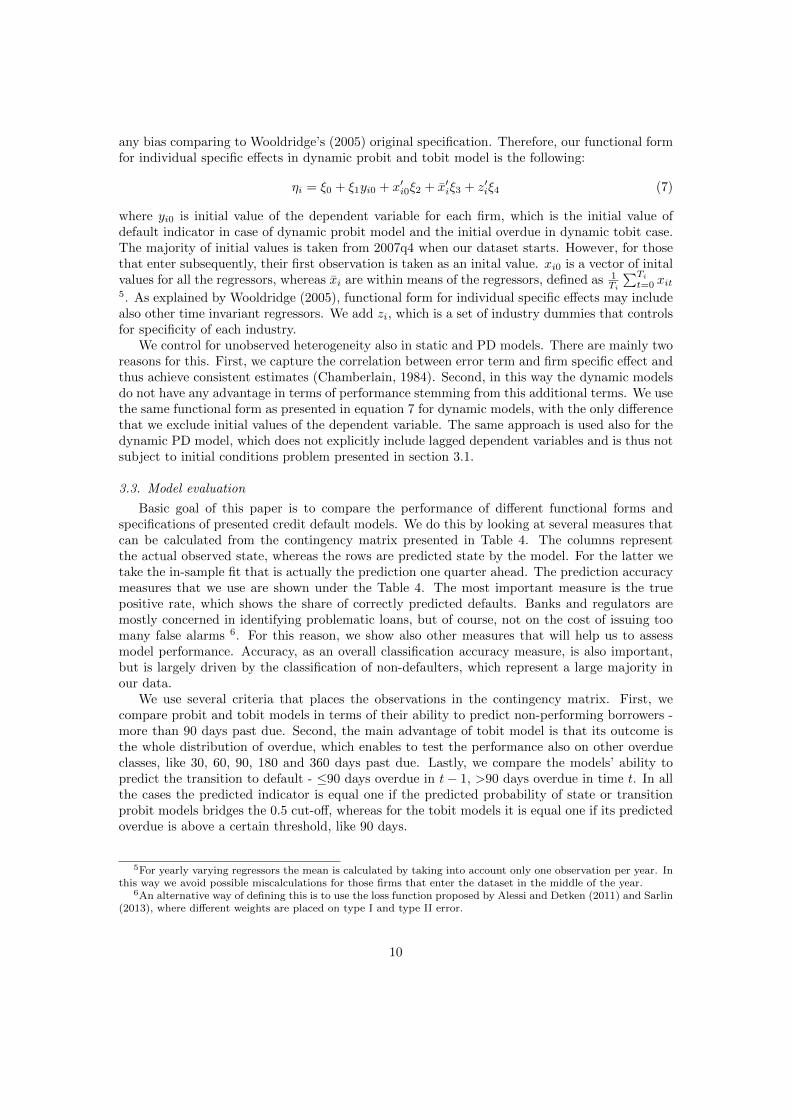
Table 5 presents the estimated coefficients of all the models. In addition to the variablesthat are shown in the table, all the models also include controls for unobserved heterogeneity aspresented in section 3.2. Most of the coefficients for these controls are statistically significant,which indicates that it is indeed important to control for these effects in order to achieve consistentestimates.

Lagged default indicator in dynamic probit model has, as expected, highly statistically sig-nificant positive effect on current value of indicator. This indicates that the default status, 0or 1, is highly persistent. Being zero in previous quarter, it is very likely it stays zero also incurrent period. On the other hand, once a firm is more than 90 days overdue it is not likely tobecome performing in the next quarter. Similarly, the positive effect of the dependent variable isalso found in dynamic tobit model, which shows that the overdue is expected to increase in time.Past information on overdue is also included in dynamic PD model in the form of dummies fordifferent classes of days past due (dummy for 0 days past due is excluded). It can be seen thathigher overdue in previous quarter adds more to the default probability. All these results are inline with the findings presented in section 2.

Table 5 also reveals the importance of using the model specification that takes into accountthe mixed frequency structure of the data. Most of the interaction terms between quarterlydummies and firm specific variables are statistically significant, especially so for static versionof the models. This indicates that the effect of yearly-observed variables on default probabilityor days past due is indeed heterogeneous across quarters. It is expected that the shorter theinformation lag, the more informative are the variables about credit default indicators. It isexactly what we find in our estimates. The majority of statistically significant coefficients canbe found for the first quarter (the terms that are not pre-multiplied with quarterly dummy inTable 5), where the information lag to the observed firm-specific variables is only one quarter.

We now turn our attention to prediction accuracy of the models. Table 6 presents theclassification accuracy of probit and tobit models in predicting non-performing borrowers. Itcan be seen that the dynamic specification of the models significantly improves the performance,especially for the probit model where the true positive rate increases by more than 30 percentagepoints comparing to static version of the model. Tobit model has even better performance.Static tobit achieves more than 33 percentage points higher true positive rate than static probitmodel, whereas dynamic tobit adds additional 3 percentage points to the classification accuracy

11

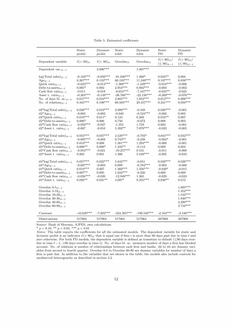
Table 5: Estimated coefficients

Static Dynamic Static Dynamic Static Dynamicprobit probit tobit tobit PD PD

I(> 90)it/ I(> 90)it/Dependent variable I(> 90)it I(> 90)it Overdueit Overdueit (≤ 90)it−1 (≤ 90)it−1

Dependent var.it−1 2.096*** 1.067***

log(Total sales)it−1 -0.182*** -0.056*** -81.820*** 1.369* 0.033** 0.004Ageit−1 0.267*** 0.133*** 60.193*** 11.249*** 0.107*** 0.038***Quick ratioit−1 -0.023*** -0.014*** -1.368*** -1.249*** -0.018*** -0.006Debt-to-assetsit−1 0.005* 0.002 2.954*** 0.802*** -0.003 -0.002Cash flow ratioit−1 -0.011 -0.018 -8.654*** -7.447*** -0.045** -0.025Asset t. ratioit−1 -0.263*** -0.149*** -26.766*** -22.156*** -0.209*** -0.076***No. of days bl. ac.it−1 0.017*** 0.010*** 2.805*** 1.053*** 0.012*** 0.006***No. of relationsit−1 0.345*** 0.198*** 69.505*** 29.457*** 0.241*** 0.050***

d2*log(Total sales)it−1 0.026*** 0.019*** 2.980*** -0.449 0.026*** -0.001d2*Ageit−1 -0.003 -0.002 -0.040 -0.524*** -0.002 0.003d2*Quick ratioit−1 0.019*** 0.011* 0.123 0.269 0.016** 0.007d2*Debt-to-assetsit−1 0.006* 0.006 0.750 -0.072 0.008 0.003d2*Cash flow ratioit−1 -0.050*** -0.027 -1.355 1.759 0.003 -0.001d2*Asset t. ratioit−1 -0.007 -0.010 5.392** 7.079*** -0.023 -0.005

d3*log(Total sales)it−1 0.053*** 0.037*** 2.529*** -0.793* 0.045*** 0.032***d3*Ageit−1 -0.005*** -0.003 0.743** -0.238 -0.004* -0.001d3*Quick ratioit−1 0.019*** 0.008 1.381*** 1.294*** -0.000 -0.001d3*Debt-to-assetsit−1 0.008** 0.008* 1.332** -0.113 0.009 0.004d3*Cash flow ratioit−1 -0.054*** -0.021 -10.257*** 0.531 -0.011 -0.008d3*Asset t. ratioit−1 0.002 0.001 1.306 5.449*** -0.005 -0.023

d4*log(Total sales)it−1 0.057*** 0.022*** 5.843*** -0.651 0.029*** 0.026***d4*Ageit−1 -0.007*** -0.003 0.099 -0.783*** -0.003 -0.000d4*Quick ratioit−1 0.019*** 0.007 1.360*** 1.256*** -0.020* -0.015d4*Debt-to-assetsit−1 0.007** 0.005 1.634*** -0.226 0.009 0.009d4*Cash flow ratioit−1 -0.056*** -0.020 -12.949*** 1.365 -0.029 -0.033d4*Asset t. ratioit−1 0.028** 0.031** 4.097* 9.355*** 0.038** 0.012

Overdue 0-5it−1 1.095***Overdue 5-10it−1 1.352***Overdue 10-20it−1 1.533***Overdue 20-30it−1 1.840***Overdue 30-60it−1 2.290***Overdue 60-90it−1 2.716***

Constant -10.629*** -7.002*** -824.385*** -190.530*** -2.164*** -2.546***

Observations 517964 517964 517964 517964 487969 487969

Source: Bank of Slovenia, AJPES, own calculations.* p < 0.10, ** p < 0.05, *** p < 0.01Notes: The table reports the coefficients for all the estimated models. The dependent variable for static anddynamic probit is an indicator I(> 90)it that is equal one if firm i is more than 90 days past due in time t andzero otherwise. For both PD models, the dependent variable is defined as transition to default (≤90 days over-due in time t− 1, >90 days overdue in time t). No. of days bl. ac. measures number of days a firm has blockedaccount. No. of relations is number of relationships between each firm and banks. d2 to d4 are dummy vari-ables from second to fourth quarter. Overdue 0-5 to Overdue 60-90 are dummy variables for number of days afirm is past due. In addition to the variables that are shown in the table, the models also include controls forunobserved heterogeneity as described in section 3.2.

12

of defaulters. Importantly, this high prediction accuracy of defaulters is not on a cost of issuingtoo many false alarms. Tobit model has slightly higher false positive rate, but these are still verylow values, especially in the case of dynamic model. Comparing to the gain in true positive rate,the loss in terms of false alarms is relatively minor.

Table 6: Performance of probit and tobit model in predicting performing and non-performing borrowers

Probit TobitStatic Dynamic Static Dynamic

True positive rate 0.356 0.663 0.688 0.714True negative rate 0.990 0.993 0.947 0.991False positive rate 0.010 0.007 0.053 0.009False negative rate 0.644 0.337 0.312 0.286Accuracy 0.949 0.972 0.930 0.973

Source: Bank of Slovenia, AJPES, own calculations.Notes: The table reports the classification performance of probit andtobit models in predicting performing and non-performing borrowers(more than 90 days past due). See section 3.3 for the description ofclassification accuracy measures.

Table 7 shows the classification accuracy of dynamic probit and dynamic tobit model inpredicting non-performing firms where we let the autoregressive process to proceed four quartersahead. These are still the in-sample predictions, with the only difference that instead of actuallyobserved values of lagged dependent variable its predictions are taken, which are obtained byrecursively running the predictions four times. The results show that tobit is the superior modelalso on a longer horizon. Its true positive rate is expectedly decreasing on longer forecast horizon,but it stays above the performance of the probit model. Dynamic probit achieves slightly higheroverall accuracy, but this is only due to better prediction of non-defaulters. False positive ratestill stays very low for both models.

Table 7: Performance of dynamic probit and tobit model in predicting performing and non-performing borrowersfrom one to four quarters ahead

Dynamic probit Dynamic tobit1q 2q 3q 4q 1q 2q 3q 4q

True positive rate 0.663 0.571 0.505 0.454 0.714 0.603 0.544 0.508True negative rate 0.993 0.992 0.993 0.993 0.991 0.987 0.986 0.986False positive rate 0.007 0.008 0.007 0.007 0.009 0.013 0.014 0.014False negative rate 0.337 0.429 0.495 0.546 0.286 0.397 0.456 0.492Accuracy 0.972 0.964 0.959 0.954 0.973 0.962 0.956 0.952

Source: Bank of Slovenia, AJPES, own calculations.Notes: The table reports the classification performance of dynamic probit and dynamic tobitmodel in predicting performing and non-performing borrowers (more than 90 days past due) oneto four quarters ahead. See section 3.3 for the description of classification accuracy measures.

Tobit model enables to form the predictions for different overdue classes. Table 8 shows theclassification accuracy results of static and dynamic tobit model for five thresholds of days pastdue. All the classes are defined in the same way: when overdue or prediction is above a certainthreshold the indicator is equal one, otherwise it is zero. It can be seen that in the case ofstatic model, true positive rate is decreasing with higher overdue threshold. The model correctlyclassifies 85% of firms with overdue above 30 days, but only 39% of firms with overdue higher

13

than 360 days. The performance of the dynamic model is much more stable and its true positiverate is fluctuating around 75%. Static model outperforms the dynamic one in terms of truepositive rate for 30 and 60 days class. It, however, also has significantly higher false positiverate, which is for the 30-days class equal to 20%, comparing to only 3% of the dynamic model.The results presented in Table 8 thus reveal, that both, static and dynamic tobit model, arequite successful in classifying borrowers to different classes of overdue, but the dynamic versionof the model is shown to be the superior one.

Table 8: Classification accuracy of static and dynamic tobit model across different groups of overdue

Static tobit Dynamic tobitOverdue threshold 30 60 90 180 360 30 60 90 180 360

True positive rate 0.854 0.752 0.688 0.561 0.390 0.746 0.720 0.714 0.733 0.774True negative rate 0.800 0.918 0.947 0.973 0.987 0.972 0.986 0.991 0.997 0.998False positive rate 0.200 0.082 0.053 0.027 0.013 0.028 0.014 0.009 0.003 0.002False negative rate 0.146 0.248 0.312 0.439 0.610 0.254 0.280 0.286 0.267 0.226Accuracy 0.805 0.906 0.930 0.953 0.967 0.952 0.967 0.973 0.984 0.991

Source: Bank of Slovenia, AJPES, own calculations.Notes: The table reports the performance of static and dynamic tobit model in classifying borrowers into differ-ent groups of days past due. In all the cases an indicator is equal one if overdue is above certain threshold (30, 60,90, 180 or 360 days past due) and zero if it is equal or below that threshold. See section 3.3 for the descriptionof classification accuracy measures.

Banks and regulators are mostly concerned about predicting new non-performing borrowers.PD as a measure of likelihood that a borrower will default on a certain horizon is also a keycredit risk parameter under the IRB capital regulation. Table 9 presents the performance of themodels in predicting the transition to default (≤90 days overdue in time t−1, >90 days overduein time t). Classical static PD model that is most frequently used in practice and where onlyfirm specific variables are used as regressors, is shown to have very low performance. It correctlyidentifies only 5% of new defaults. Extending the model with dummies for different classes ofoverdue in t − 1 significantly improves the performance to 27% true positive rate. This is tobe expected since, as we already presented in section 2, past information on days past due isvery informative about current default status. The higher the overdue in previous quarter, morelikely it is that the firm defaults in current period. A minor change in the model can thus leadto much more accurate estimates of the default probability.

Table 9: Models’ performance in predicting transition to default

Static Dynamic Static Dynamic Static DynamicPD PD probit probit tobit tobit

True positive rate 0.047 0.274 0.150 0.045 0.501 0.139True negative rate 0.997 0.997 0.991 0.997 0.950 0.995False positive rate 0.003 0.003 0.009 0.003 0.050 0.005False negative rate 0.953 0.726 0.850 0.955 0.499 0.861Accuracy 0.983 0.986 0.979 0.983 0.943 0.983

Source: Bank of Slovenia, AJPES, own calculations.Notes: The table reports the performance of the estimated models in predicting the transi-tion to default (≤90 days overdue in time t− 1, >90 days overdue in time t).

The performance in predicting new defaulters can also be calculated for the models whereeither state of default or overdue is used as the dependent variable. It is interesting to find that

14

any other version of the model outperforms the classical PD model. The only exception is thedynamic probit model, where the autoregressive term leads to persistence of states and thereis thus not a lot of switching between performing and non-performing states. 7 As expected,the dynamic tobit with lagged information about days past due is better able to capture thetransition to default, but however, is still performing worse than some other models. It seemsthat the autoregressive component is not strong enough to lead to a sufficient increase of overduebetween two consecutive periods.

The best performing model for predicting transition to default is found to be the statictobit. It achieves 50% classification accuracy of new defaulters and outperforms all other modelsby a large margin. It also has the highest false positive rate (5%), which also explains loweroverall accuracy. This measure, however, is typically not of a primary interest in evaluatingthe performance of default probability models and comparing to the gain in correctly identifyingdefaulters, the loss of over-signalling is relatively small. We formally compare the performance ofthe two best performing models, dynamic PD and static tobit, using the methodology proposedby Alessi and Detken (2011). Applying equal weights on type 1 and type 2 error results in a lossof 0.365 for dynamic PD and only 0.275 for static tobit. Given that regulators and banks aretypically more concerned about missing the defaulters than issuing false alarms, which would bereflected in higher weight on type 1 error, places the static tobit model to even more superiorposition.

Let us summarize our main results. We find two strong peace of evidence that the tobitmodelling technique of credit risk is the advantageous one. Dynamic tobit model is shownto achieve the best classification accuracy of non-performing borrowers, whereas static tobitoutperforms all the other models in predicting new defaulters. The advantage of tobit model isalso that it enables classifying borrowers to different groups of overdue and thus get the wholespectrum of riskiness of credit portfolio. We also show that the static PD model, that is widelyused by banks and regulators, actually has the worst classifying performance. Given the evidencein our paper, it thus seems reasonable to upgrade credit risk modelling techniques, since theselead to much more accurate predictions. We now check the robustness of our results.

5. Robustness checks

This section presents three sets of robustness checks. First, we show the out-of-sample per-formance results. Second, we extend the horizon in PD models from one quarter to one year.Third, we show the dynamic model predictions on a sub-sample of firms that are present at thebeginning of the sample.

5.1. Out-of-sample performance

The classification accuracy results presented thus far are in-sample predictions. Models aretypically used to forecast credit default on a certain horizon. We therefore check the validity ofour results by also predicting out-of-sample. We do this by recursively estimating the modelsand predicting the state of default or overdue one quarter ahead. For instance, we estimatethe models until 2010q4 and forecast 2011q1. We start the estimating process in 2008q4, suchthat we get the estimates for all the coefficients, including the interactions between quarterlydummies and firm specific variables. The applied estimating methodology, however, needs tobe simplified due to a large computational burden. Using random effects estimator, it took the

7As shown in Table 6, dynamic probit achieves a high accuracy in predicting non-performing borrowers, wherethe persistence of both states is of a key importance.

15

computer approximately 12 days to estimate all the models presented in Table 5. Given thatnow all the estimates would need to be replicated 24-times, it would take a very long time toestimate all the models. We therefore use pooled estimators, which proceed much faster. Theonly difference comparing to random effects estimator is that the pooled version is less efficient,since it does not take into account the autoregressive structure of the variance-covariance matrix.Since we use an alternative methodology, the prediction accuracy of this procedure should notbe directly compared to the results presented in previous section.

Table 10 presents the out-of-sample performance in predicting non-performing borrowers.Even though the estimation methodology is now different, the prediction accuracy is similar aspresented in Table 6 for in-sample predictions. Similarly, we also find that the dynamic versionof the models outperform the static ones. Dynamic probit achieves the highest classificationaccuracy of defaulters (78%) with low false positive rate below 1%. This model, however, is notable to break down firms to different overdue classes. Table 11 displays these results for staticand dynamic tobit. Similar as before, we find that the predictions of the dynamic model aremuch more stable and accurate.

Table 10: Out-of-sample performance of probit and tobit model in predicting performing and non-performingborrowers

Probit TobitStatic Dynamic Static Dynamic

True positive rate 0.396 0.783 0.710 0.721True negative rate 0.990 0.992 0.951 0.992False positive rate 0.010 0.008 0.049 0.008False negative rate 0.604 0.217 0.290 0.279Accuracy 0.949 0.978 0.935 0.974

Source: Bank of Slovenia, AJPES, own calculations.Notes: The table reports the out-of-sample classification perfor-mance of probit and tobit models in predicting performing and non-performing borrowers (more than 90 days past due). See section 3.3for the description of classification accuracy measures.

Table 11: Out-of-sample classification accuracy of static and dynamic tobit model across different groups ofoverdue

Static tobit Dynamic tobitOverdue threshold 30 60 90 180 360 30 60 90 180 360

True positive rate 0.887 0.777 0.710 0.592 0.427 0.751 0.725 0.721 0.739 0.780True negative rate 0.776 0.923 0.951 0.975 0.988 0.975 0.988 0.992 0.997 0.998False positive rate 0.224 0.077 0.049 0.025 0.012 0.025 0.012 0.008 0.003 0.002False negative rate 0.113 0.223 0.290 0.408 0.573 0.249 0.275 0.279 0.261 0.220Accuracy 0.786 0.911 0.935 0.955 0.969 0.955 0.968 0.974 0.983 0.991

Source: Bank of Slovenia, AJPES, own calculations.Notes: The table reports the out-of-sample performance of static and dynamic tobit model in classifying borrow-ers into different groups of days past due. In all the cases an indicator is equal one if overdue is above certainthreshold (30, 60, 90, 180 or 360 days past due) and zero if it is equal or below that threshold. See section 3.3 forthe description of classification accuracy measures.

We now turn to out-of-sample prediction accuracy of new defaulters. The results presentedin Table 12 reveal that the prevailing modelling methodology, static PD model, performs very

16

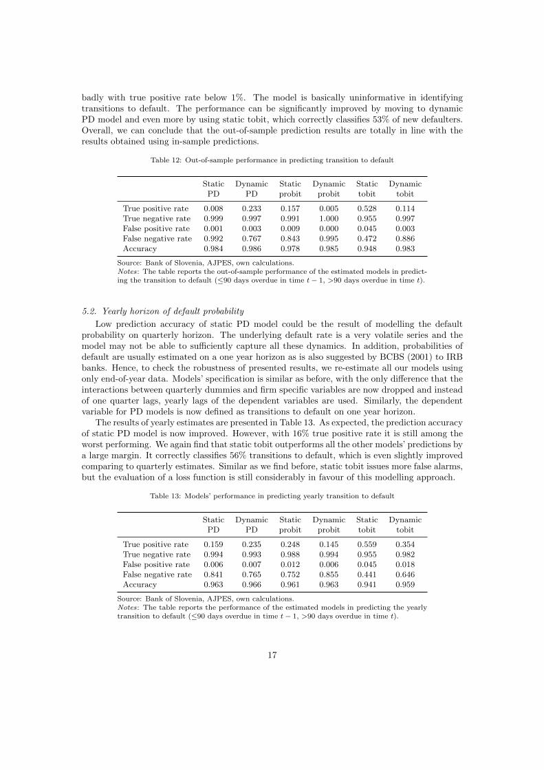
badly with true positive rate below 1%. The model is basically uninformative in identifyingtransitions to default. The performance can be significantly improved by moving to dynamicPD model and even more by using static tobit, which correctly classifies 53% of new defaulters.Overall, we can conclude that the out-of-sample prediction results are totally in line with theresults obtained using in-sample predictions.

Table 12: Out-of-sample performance in predicting transition to default



Source: Bank of Slovenia, AJPES, own calculations.Notes: The table reports the out-of-sample performance of the estimated models in predict-ing the transition to default (≤90 days overdue in time t− 1, >90 days overdue in time t).

5.2. Yearly horizon of default probability

Low prediction accuracy of static PD model could be the result of modelling the defaultprobability on quarterly horizon. The underlying default rate is a very volatile series and themodel may not be able to sufficiently capture all these dynamics. In addition, probabilities ofdefault are usually estimated on a one year horizon as is also suggested by BCBS (2001) to IRBbanks. Hence, to check the robustness of presented results, we re-estimate all our models usingonly end-of-year data. Models’ specification is similar as before, with the only difference that theinteractions between quarterly dummies and firm specific variables are now dropped and insteadof one quarter lags, yearly lags of the dependent variables are used. Similarly, the dependentvariable for PD models is now defined as transitions to default on one year horizon.

The results of yearly estimates are presented in Table 13. As expected, the prediction accuracyof static PD model is now improved. However, with 16% true positive rate it is still among theworst performing. We again find that static tobit outperforms all the other models’ predictions bya large margin. It correctly classifies 56% transitions to default, which is even slightly improvedcomparing to quarterly estimates. Similar as we find before, static tobit issues more false alarms,but the evaluation of a loss function is still considerably in favour of this modelling approach.

Table 13: Models’ performance in predicting yearly transition to default



Source: Bank of Slovenia, AJPES, own calculations.Notes: The table reports the performance of the estimated models in predicting the yearlytransition to default (≤90 days overdue in time t− 1, >90 days overdue in time t).

17

5.3. Dynamic model estimates on a sub-sample of firms

Wooldridge’s (2005) methodology, which we use to estimate the dynamic models, requiresthat the estimates are performed on a balanced panel data.8 Due to the nature of the modellingproblem, our panel is unbalanced. Firms that become overdue on their credit obligation sooneror later bankrupt and disappear from the sample. In addition, new firms are entering into thesample. In applied work researchers usually estimate the dynamic models only on balanced partof the data set (see for instance O’Neill and Hanrahan, 2011). In our case, however, this wouldlead to serious sample selection bias. We would be mostly left with the firms that defaultedduring the last periods of the sample. We rely on the evidence provided by Akay (2009), whoshows by simulations that using Wooldridge’s (2005) methodology on unbalanced panel does notlead to any serious bias. In addition, we also estimate our models on a sub-sample of firmsthat are represented at the beginning of the sample. We therefore exclude all the firms thatsubsequently enter the dataset. In this way we achieve that the initial values for all the firmsare taken from the same time period (2007q4).

Table 14 presents the performance results of dynamic probit and tobit models estimatedon a sample of firms present in 2007q4. As it can be seen, this only marginally changes theclassification accuracy results. We can still find that the dynamic models outperform the staticones and that the dynamic tobit is the advantageous methodology for identifying non-performingborrowers. Overall, the results are in line with the findings presented in section 4.

Table 14: Performance of the dynamic models estimated on a sub-sample of firms

Dynamic Dynamic tobitprobit 30 60 90 180 360


Source: Bank of Slovenia, AJPES, own calculations.Notes: The table reports the performance of dynamic probit and tobit model es-timated on a sample of firms present at the beginning of the sample (2007q4).Dynamic probit performance is shown for the 90 days overdue threshold, whereasdynamic tobit results are for different thresholds from 30 to 360 days.

6. Conclusion

In this paper we evaluate the performance of several credit default models, which are com-pared in their ability to correctly predict non-performing borrowers and transitions to default.In addition to conventional static binary models, we also evaluate the performance of two novelmethodologies that, to our knowledge, have not yet been applied in modelling credit risk. Over-due in loan repayment is already a risk measure and therefore it seems reasonable to estimate itdirectly, using the tobit model methodology. In addition, state of default and overdue are highlyautoregressive processes. Overdue is expected to increase in time, whereas state of default showsa lot of persistence. Estimating the dynamic probit and tobit model, where lagged dependentvariable is included among regressors, can significantly improve the performance of the model.

8Honore (2002) shows that the initial conditions problem is especially problematic in unbalanced panels.

18

Same inputs are used in all the models, which means that the differences in classification accuracycan be fully attributed to different functional forms (probit vs. tobit) and additional informationthat enter the model in the form of lagged dependent variable.

We show that tobit modelling methodology outperforms all other methodologies. Dynamictobit model is shown to achieve the highest classification accuracy in predicting non-performingborrowers. It correctly identifies more than 70% of defaulters and issues less than 1% of falsealarms. In addition, its prediction is number of days past due, which enables to form differentclasses of overdue. This is a very valuable information, since it gives direct and easily interpretableinformation on expected portfolio riskiness. We show that tobit model performance is very highand stable across different overdue classes, from 30 to 360 days. High performance (66% truepositive rate) is also achieved by dynamic probit, which outperforms the static version by morethan 30 percentage points. This shows that the dynamic modelling methodology can significantlyimprove the performance of credit default models.

Tobit model also has the highest prediction ability for explaining transitions to default. Inclassifying firms into performing and non-performing class the dynamic structure of the modelplays a crucial role. When a certain overdue threshold is bridged, it is not very likely thatthe borrower will become performing again. In explaining transitions to default, however, thisautoregressive process is too slow to sufficiently capture the increase of overdue from one quarterto another. We therefore find the static tobit model to perform the best in terms of true positiverate. It correctly classifies 50% of new defaulters and outperforms all other models by a largemargin. It also issues more false alarms, but as we show, the evaluation of loss function, whichtakes into account type I and type II error, is much in favour of this model. On the other hand,conventional PD model, that is typically used by banks and regulators, has very low performance.It is able to correctly identify only 5% of transitions to default. A number of robustness checksconfirm the validity of our results.

The findings in this paper have several important implications for banks, banking regula-tion and credit risk modelling practitioners. We show that the prevailing credit risk modellingmethodology, which is based on binary classifiers, can be significantly improved by including thedynamics and choosing the tobit functional form of the model. In addition, we propose a modelspecification to estimate credit risk on a quarterly basis, which enables much more frequent andaccurate monitoring of expected changes in credit portfolio.

A more important finding of our empirical analysis is very low prediction performance ofconventional static PD model. This type of model is usually used by banks to assess riskiness oftheir portfolio and to determine one of the crucial parameters for calculating capital requirementsunder IRB regulation - the probability of default. A simple upgrade of the model with dummiesindicating overdue in previous period significantly improves the performance. Even higher pre-diction ability is achieved by static tobit model. Although the prediction of this model is not inthe form of default probability and can thus not be directly used in IRB formula, it seems veryuseful for identifying new defaulters more accurately. This is important information for banksand regulators, since knowing which borrowers are expected to default in next period they areable to assess in advance the required loan loss provisions and capital to cover the losses. Inaddition, IRB regulation (BCBS, 2001) requires from banks to form classes of default probabilityand apply the same PD to all the firms within the class. Tobit predictions enable to form similarriskiness classes based on days past due. Combining this predictions with the information aboutdefault rate for each overdue class, one can, similarly as under IRB regulation, also attach defaultprobability to each class.

19

References

[1] Akay A. (2009). The Wooldridge Method for the Initial Values Problem Is Simple: WhatAbout Performance? Discussion Paper No. 3943, Institute for the Study of Labor (IZA),Bonn.

[2] Akay A. (2012). Finite-sample comparison of alternative methods for estimating dynamicpanel data models. Journal of Applied Econometrics, 27, 1189-1204.

[3] Alessi L. & Detken C. (2011). Quasi real time early warning indicators for costly asset priceboom/bust cycles: A role for global liquidity. European Journal of Political Economy, 27,520-533.

[4] Altman E. (1968). Financial ratios, discriminant analysis and the prediction of corporatebankruptcy. The Journal of Finance, 23 (4), 589-609.

[5] Anderson T.W. & Hsiao C. (1982). Formulation and estimation of dynamic models usingpanel data. Journal of Econometrics, 18, 67-82.

[6] Arellano M. & Bond S.R. (1991). Some tests of specification for panel data: Monte Carloevidence and an application to employment equations. Review of Economic Studies, 58,277-297.

[7] Arellano M. & Carrasco R. (2003). Binary choice panel data models with predeterminedvariables. Journal of Econometrics, 115, 125-157.

[8] BCBS (2001). The Internal-Rating Based Approach. Supporting Document to the New BaselCapital Accord.

[9] BCBS (2006). International Convergence of Capital Measurements and Capital Standards:A Revised Framework Comprehensive Version.

[10] Blundell R. & Bond S. (1998). Initial conditions and moment restrictions in dynamic paneldata models. Journal of Econometrics, 87, 115-143.

[11] Bonfim D. (2009). Credit risk drivers: Evaluating the contribution of firm level informationand of macroeconomic dynamics. Journal of Banking & Finance, 33, 281-299.

[12] Carling K., Jacobson T., Linde J. & Roszbach K. (2007). Corporate credit risk modelingand the macroeconomy. Journal of Banking & Finance, 31, 845-868.

[13] Chamberlain G. (1984). Panel data. In Handbook of Econometrics, Vol. 2, Griliches Z.,Intriligator M. North-Holland, Amsterdam, 1247-1318.

[14] Costeiu A. & Neagu F. (2013). Bridging the banking sector with the real economy. A financialstability perspective. ECB Working Paper Series, No. 1592.

[15] Hamerle A., Liebig T. & Rosch D. (2003). Credit risk factor modeling and the Basel II IRBapproach. Deutsche Bundesbank Discussion Paper, No. 02/2003.

[16] Heckman J.J. (1981a). Heterogeneity and state dependence. In Studies in Labor Markets,Rosen S. University of Chicago Press, 91-139.

[17] Heckman J.J. (1981b). The incidental parameters problem and the problem of initial condi-tions in estimating a discrete time-discrete data stochastic process. In Structural Analysis ofDiscrete Data with Econometric Applications, Manski C., McFadden D, MIT Press, 114-178.

20

[18] Honore B. (2002). Nonlinear models with panel data. Portuguese Economic Journal, 1,163-179.

[19] Honore B. & Kyriazidou E. (2000). Panel data discrete choice models with lagged dependentvariables. Econometrica, 68, 839-874.

[20] Jones S., Johnstone D. & Wilson R. (2015). An empirical evaluation of the performance ofbinary classifiers in the prediction of credit rating changes. Journal of Banking & Finance,56, 72-85.

[21] Neyman J. & Scott E. (1948). Consistent estimates based on partially consistent observa-tions. Econometrica, 16, 1-32.

[22] O’Neill S. & Hanrahan K. (2012). Decoupling of agricultural support payments: the impacton land market participation decisions. European Review of Agricultural Economics, 39 (4),639-659.

[23] Rabe-Hesketh S. & Skrondal A. (2013). Avoiding biased versions of Wooldridge’s simplesolution to the initial conditions problem. Economics Letters, 120, 346-349.

[24] Sarlin P. (2013). On policymakers loss functions and the evaluation of early warning systems.Economics Letters, 119 (1), 1-7.

[25] Volk M. (2012). Estimating Probability of Default and Comparing it to Credit Rating Clas-sification by Banks. Economic and Business Review, 14 (4), 299-320.

[26] Wooldridge J.M. (2005). Simple solution to the initial conditions problem in dynamic, non-linear panel data models with unobserved heterogeneity. Journal of Applied Econometrics,20, 39-54.

21

Documents

Evaluating the Performance of Dynamic and Tobit …economics.soc.uoc.gr/macro/docs/Year/2016/papers/paper_3_183.pdf · Evaluating the Performance of Dynamic and Tobit Models in Predicting