SANDIA REPORTSAND2016-8845Unlimited ReleasePrinted September, 2016

Evaluating the Opportunities forMulti-Level Memory – An ASC 2016 L2MilestoneG.R. Voskuilen, M.P. Frank, S.D. Hammond, and A.F. Rodrigues

Center for Computing ResearchSandia National LaboratoriesAlbuquerque, NM, 87185

Prepared bySandia National LaboratoriesAlbuquerque, New Mexico 87185 and Livermore, California 94550

Sandia National Laboratories is a multi-mission laboratory managed and operated by Sandia Corporation,a wholly owned subsidiary of Lockheed Martin Corporation, for the U.S. Department of Energy’sNational Nuclear Security Administration under contract DE-AC04-94AL85000.

Approved for public release; further dissemination unlimited.

Issued by Sandia National Laboratories, operated for the United States Department of Energyby Sandia Corporation.

NOTICE: This report was prepared as an account of work sponsored by an agency of the UnitedStates Government. Neither the United States Government, nor any agency thereof, nor anyof their employees, nor any of their contractors, subcontractors, or their employees, make anywarranty, express or implied, or assume any legal liability or responsibility for the accuracy,completeness, or usefulness of any information, apparatus, product, or process disclosed, or rep-resent that its use would not infringe privately owned rights. Reference herein to any specificcommercial product, process, or service by trade name, trademark, manufacturer, or otherwise,does not necessarily constitute or imply its endorsement, recommendation, or favoring by theUnited States Government, any agency thereof, or any of their contractors or subcontractors.The views and opinions expressed herein do not necessarily state or reflect those of the UnitedStates Government, any agency thereof, or any of their contractors.

Printed in the United States of America. This report has been reproduced directly from the bestavailable copy.

Available to DOE and DOE contractors fromU.S. Department of EnergyOffice of Scientific and Technical InformationP.O. Box 62Oak Ridge, TN 37831

Telephone: (865) 576-8401Facsimile: (865) 576-5728E-Mail: reports@adonis.osti.govOnline ordering: http://www.osti.gov/bridge

Available to the public fromU.S. Department of CommerceNational Technical Information Service5285 Port Royal RdSpringfield, VA 22161

Telephone: (800) 553-6847Facsimile: (703) 605-6900E-Mail: orders@ntis.fedworld.govOnline ordering: http://www.ntis.gov/help/ordermethods.asp?loc=7-4-0#online

DE

PA

RT

MENT OF EN

ER

GY

• • UN

IT

ED

STATES OFA

M

ER

IC

A

2

SAND2016-8845Unlimited Release

Printed September, 2016

Evaluating the Opportunities for Multi-Level Memory – An ASC

2016 L2 Milestone

G.R. Voskuilen, M. Frank, S.D. Hammond, and A.F. RodriguesCenter for Computing ResearchSandia National LaboratoriesAlbuquerque, NM, 87185

The next two Advanced Technology platforms for the ASC program will feature complex memory hierarchies– in the Trinity supercomputer being deployed in 2016, Intel’s Knights Landing processors will feature 16GBof on-package, high-bandwidth memory, combined with a larger capacity DDR4 memory and in 2018, theSierra machine deployed at Lawrence Livermore National Laboratory will feature powerful compute nodescontaining POWER9 processors with large capacity memories and an array of coherent GPU acceleratorsalso with high bandwidth memories.

In this ASC L2 milestone we report on a spectrum of studies investigating the potential performanceopportunities of multi-level memory systems which might utilize hardware accelerated caching or, alterna-tively, entirely software driven management either by an application or allocation/memory aware runtime.As the basis for our exploration we utilize several of the APEX ASC benchmarks currently planned to beused in the ATS-3 Crossroads procurement in late 2016.

Our studies investigate issues of system balance, memory size, cache sizes and a number of other key hard-ware parameters. We show that although a number of benchmark kernels are not bound by the bandwidthof memory in the system and so experience no significant improvement in runtime from higher-bandwidthor on-package memories, other kernels, particularly those relating to sparse linear algebra can experiencesignificant acceleration due to their poor data reuse properties and low ratio of compute operations.

We conclude that multi-level memories provide a very varied picture for the performance of codes onfuture systems and highlight areas where application programmers and computational scientists may wantto focus their efforts.

3

Acknowledgment

Sandia National Laboratories is a multi-mission laboratory managed and operated by Sandia Corporation,a wholly owned subsidiary of Lockheed Martin Corporation, for the U.S. Department of Energy’s NationalNuclear Security Administration under contract DE-AC04-94AL85000.

This report represents a significant extension to Sandia’s Structural Simulation Toolkit that build uponcontributions and inputs from the whole SST project team.

Results from the ASC Test Beds draw on work from our diligent system administration teams. We aregrateful for their continued support for our work.

4

Contents

1 Introduction 11

1.1 Multi-Level Memory Systems . . . . . . . . . . . . . . . . . . . . . . . . . . . . . . . . . . . . . . . . . . . . . . . . . . . . . 11

1.1.1 The Case For... . . . . . . . . . . . . . . . . . . . . . . . . . . . . . . . . . . . . . . . . . . . . . . . . . . . . . . . . . . . 11

Economic Impacts . . . . . . . . . . . . . . . . . . . . . . . . . . . . . . . . . . . . . . . . . . . . . . . . . . . . . . . . 11

Analysis . . . . . . . . . . . . . . . . . . . . . . . . . . . . . . . . . . . . . . . . . . . . . . . . . . . . . . . . . . . . . . . . 12

1.1.2 The Case Against... . . . . . . . . . . . . . . . . . . . . . . . . . . . . . . . . . . . . . . . . . . . . . . . . . . . . . . . 13

Economics . . . . . . . . . . . . . . . . . . . . . . . . . . . . . . . . . . . . . . . . . . . . . . . . . . . . . . . . . . . . . . . 13

Management . . . . . . . . . . . . . . . . . . . . . . . . . . . . . . . . . . . . . . . . . . . . . . . . . . . . . . . . . . . . . 13

Latency . . . . . . . . . . . . . . . . . . . . . . . . . . . . . . . . . . . . . . . . . . . . . . . . . . . . . . . . . . . . . . . . . 13

1.2 Three Paths to MLM Management . . . . . . . . . . . . . . . . . . . . . . . . . . . . . . . . . . . . . . . . . . . . . . . . 13

1.2.1 Algorithmic . . . . . . . . . . . . . . . . . . . . . . . . . . . . . . . . . . . . . . . . . . . . . . . . . . . . . . . . . . . . . 14

1.2.2 Manual . . . . . . . . . . . . . . . . . . . . . . . . . . . . . . . . . . . . . . . . . . . . . . . . . . . . . . . . . . . . . . . . . 14

1.2.3 Automatic . . . . . . . . . . . . . . . . . . . . . . . . . . . . . . . . . . . . . . . . . . . . . . . . . . . . . . . . . . . . . . . 15

1.3 Roadmap . . . . . . . . . . . . . . . . . . . . . . . . . . . . . . . . . . . . . . . . . . . . . . . . . . . . . . . . . . . . . . . . . . . . . 15

2 Methodology 17

2.1 Applications . . . . . . . . . . . . . . . . . . . . . . . . . . . . . . . . . . . . . . . . . . . . . . . . . . . . . . . . . . . . . . . . . . . 17

2.1.1 Methodology for Simulating at Scale . . . . . . . . . . . . . . . . . . . . . . . . . . . . . . . . . . . . . . . . . 19

2.2 Simulation . . . . . . . . . . . . . . . . . . . . . . . . . . . . . . . . . . . . . . . . . . . . . . . . . . . . . . . . . . . . . . . . . . . . 19

2.2.1 Simulation Improvements . . . . . . . . . . . . . . . . . . . . . . . . . . . . . . . . . . . . . . . . . . . . . . . . . . 21

2.2.2 Architectures . . . . . . . . . . . . . . . . . . . . . . . . . . . . . . . . . . . . . . . . . . . . . . . . . . . . . . . . . . . . 21

2.2.3 Validation . . . . . . . . . . . . . . . . . . . . . . . . . . . . . . . . . . . . . . . . . . . . . . . . . . . . . . . . . . . . . . . 22

3 Design Space Exploration 25

3.1 Potential Performance with HMC . . . . . . . . . . . . . . . . . . . . . . . . . . . . . . . . . . . . . . . . . . . . . . . . . 25

3.2 Validating the Lightweight Model . . . . . . . . . . . . . . . . . . . . . . . . . . . . . . . . . . . . . . . . . . . . . . . . . . 26

3.3 Latency and Bandwidth Sensitivity . . . . . . . . . . . . . . . . . . . . . . . . . . . . . . . . . . . . . . . . . . . . . . . . 26

5

4 Manual Management 29

4.1 Software Approaches & Trade-offs . . . . . . . . . . . . . . . . . . . . . . . . . . . . . . . . . . . . . . . . . . . . . . . . . 29

4.1.1 Trade-offs . . . . . . . . . . . . . . . . . . . . . . . . . . . . . . . . . . . . . . . . . . . . . . . . . . . . . . . . . . . . . . . 30

4.1.2 Options Explored . . . . . . . . . . . . . . . . . . . . . . . . . . . . . . . . . . . . . . . . . . . . . . . . . . . . . . . . . 31

4.2 MemSieve: A tool for profiling application memory behavior . . . . . . . . . . . . . . . . . . . . . . . . . . . 31

4.2.1 The MemSieve Tool . . . . . . . . . . . . . . . . . . . . . . . . . . . . . . . . . . . . . . . . . . . . . . . . . . . . . . . 31

Validation . . . . . . . . . . . . . . . . . . . . . . . . . . . . . . . . . . . . . . . . . . . . . . . . . . . . . . . . . . . . . . . 32

4.2.2 Analysis . . . . . . . . . . . . . . . . . . . . . . . . . . . . . . . . . . . . . . . . . . . . . . . . . . . . . . . . . . . . . . . . 32

Malloc Characteristics . . . . . . . . . . . . . . . . . . . . . . . . . . . . . . . . . . . . . . . . . . . . . . . . . . . . . 33

Ideal Malloc Behavior . . . . . . . . . . . . . . . . . . . . . . . . . . . . . . . . . . . . . . . . . . . . . . . . . . . . . 34

Architecture Effect on Dense Mallocs . . . . . . . . . . . . . . . . . . . . . . . . . . . . . . . . . . . . . . . . 36

Dense Mallocs: What are they? . . . . . . . . . . . . . . . . . . . . . . . . . . . . . . . . . . . . . . . . . . . . . 37

Translating MemSieve to Hardware . . . . . . . . . . . . . . . . . . . . . . . . . . . . . . . . . . . . . . . . . . 38

Processing-In-Memory and MemSieve . . . . . . . . . . . . . . . . . . . . . . . . . . . . . . . . . . . . . . . . 38

4.3 Comparing Software Allocation Strategies . . . . . . . . . . . . . . . . . . . . . . . . . . . . . . . . . . . . . . . . . . . 39

4.3.1 Comparing Software Approaches . . . . . . . . . . . . . . . . . . . . . . . . . . . . . . . . . . . . . . . . . . . . 40

4.3.2 Effectiveness of Manual Allocation . . . . . . . . . . . . . . . . . . . . . . . . . . . . . . . . . . . . . . . . . . . 41

4.3.3 Effect of the Architecture . . . . . . . . . . . . . . . . . . . . . . . . . . . . . . . . . . . . . . . . . . . . . . . . . . 42

4.3.4 Conclusions . . . . . . . . . . . . . . . . . . . . . . . . . . . . . . . . . . . . . . . . . . . . . . . . . . . . . . . . . . . . . . 42

5 Automatic Management 45

5.1 Background . . . . . . . . . . . . . . . . . . . . . . . . . . . . . . . . . . . . . . . . . . . . . . . . . . . . . . . . . . . . . . . . . . . 45

5.1.1 Related Work . . . . . . . . . . . . . . . . . . . . . . . . . . . . . . . . . . . . . . . . . . . . . . . . . . . . . . . . . . . . 45

5.1.2 Key Differences . . . . . . . . . . . . . . . . . . . . . . . . . . . . . . . . . . . . . . . . . . . . . . . . . . . . . . . . . . 45

5.2 Early Analysis . . . . . . . . . . . . . . . . . . . . . . . . . . . . . . . . . . . . . . . . . . . . . . . . . . . . . . . . . . . . . . . . . 46

5.2.1 Access Patterns Within A Page . . . . . . . . . . . . . . . . . . . . . . . . . . . . . . . . . . . . . . . . . . . . . 46

5.2.2 Multithreaded Access . . . . . . . . . . . . . . . . . . . . . . . . . . . . . . . . . . . . . . . . . . . . . . . . . . . . . 46

5.3 Policies . . . . . . . . . . . . . . . . . . . . . . . . . . . . . . . . . . . . . . . . . . . . . . . . . . . . . . . . . . . . . . . . . . . . . . . 48

5.3.1 Addition Policies . . . . . . . . . . . . . . . . . . . . . . . . . . . . . . . . . . . . . . . . . . . . . . . . . . . . . . . . . 48

5.3.2 Replacement Policies . . . . . . . . . . . . . . . . . . . . . . . . . . . . . . . . . . . . . . . . . . . . . . . . . . . . . . 49

5.4 Early Results . . . . . . . . . . . . . . . . . . . . . . . . . . . . . . . . . . . . . . . . . . . . . . . . . . . . . . . . . . . . . . . . . . 49

5.4.1 Analysis . . . . . . . . . . . . . . . . . . . . . . . . . . . . . . . . . . . . . . . . . . . . . . . . . . . . . . . . . . . . . . . . 50

6

5.5 Large Application Results . . . . . . . . . . . . . . . . . . . . . . . . . . . . . . . . . . . . . . . . . . . . . . . . . . . . . . . . 50

5.5.1 Performance Vs. Policy . . . . . . . . . . . . . . . . . . . . . . . . . . . . . . . . . . . . . . . . . . . . . . . . . . . . 54

5.5.2 Fine Tuning . . . . . . . . . . . . . . . . . . . . . . . . . . . . . . . . . . . . . . . . . . . . . . . . . . . . . . . . . . . . . 54

5.5.3 Cost & Performance . . . . . . . . . . . . . . . . . . . . . . . . . . . . . . . . . . . . . . . . . . . . . . . . . . . . . . 56

5.5.4 Overheads . . . . . . . . . . . . . . . . . . . . . . . . . . . . . . . . . . . . . . . . . . . . . . . . . . . . . . . . . . . . . . . 56

5.5.5 Comparison to Manual Management . . . . . . . . . . . . . . . . . . . . . . . . . . . . . . . . . . . . . . . . . 56

6 Conclusions & Future Work 67

6.1 Conclusions . . . . . . . . . . . . . . . . . . . . . . . . . . . . . . . . . . . . . . . . . . . . . . . . . . . . . . . . . . . . . . . . . . . . 67

6.2 Future Work . . . . . . . . . . . . . . . . . . . . . . . . . . . . . . . . . . . . . . . . . . . . . . . . . . . . . . . . . . . . . . . . . . . 68

6.2.1 Manual Management . . . . . . . . . . . . . . . . . . . . . . . . . . . . . . . . . . . . . . . . . . . . . . . . . . . . . . 68

6.2.2 Automatic Management . . . . . . . . . . . . . . . . . . . . . . . . . . . . . . . . . . . . . . . . . . . . . . . . . . . 68

6.3 Recommendations . . . . . . . . . . . . . . . . . . . . . . . . . . . . . . . . . . . . . . . . . . . . . . . . . . . . . . . . . . . . . . 69

References 70

7

List of Figures

1.1 Address histograms sorted by address . . . . . . . . . . . . . . . . . . . . . . . . . . . . . . . . . . . . . . . . . . . . . . 14

2.1 Generic SST configuration . . . . . . . . . . . . . . . . . . . . . . . . . . . . . . . . . . . . . . . . . . . . . . . . . . . . . . . . 20

2.2 An SST configuration with Ariel, MemHierarchy, and Merlin . . . . . . . . . . . . . . . . . . . . . . . . . . . 20

2.3 Architectures studied . . . . . . . . . . . . . . . . . . . . . . . . . . . . . . . . . . . . . . . . . . . . . . . . . . . . . . . . . . . . 22

2.4 Studied access patterns: links access areas of their local quads (top) and links access the samearea in a single quad (bottom) . . . . . . . . . . . . . . . . . . . . . . . . . . . . . . . . . . . . . . . . . . . . . . . . . . . . 23

2.5 GoblinHMC validation study . . . . . . . . . . . . . . . . . . . . . . . . . . . . . . . . . . . . . . . . . . . . . . . . . . . . . 23

2.6 Sandy Bridge socket validation study . . . . . . . . . . . . . . . . . . . . . . . . . . . . . . . . . . . . . . . . . . . . . . . 24

3.1 All-HMC performance for the heavyweight architecture . . . . . . . . . . . . . . . . . . . . . . . . . . . . . . . . 25

3.2 All-HMC performance for the lightweight architecture . . . . . . . . . . . . . . . . . . . . . . . . . . . . . . . . . 26

3.3 All-HMC performance for the simulated lightweight architecture compared to a Knight’s Land-ing hardware testbed . . . . . . . . . . . . . . . . . . . . . . . . . . . . . . . . . . . . . . . . . . . . . . . . . . . . . . . . . . . . 27

3.4 Bandwidth & latency sensitivity . . . . . . . . . . . . . . . . . . . . . . . . . . . . . . . . . . . . . . . . . . . . . . . . . . . 27

4.1 MemSieve tool . . . . . . . . . . . . . . . . . . . . . . . . . . . . . . . . . . . . . . . . . . . . . . . . . . . . . . . . . . . . . . . . . 32

4.7 PENNANT: similarity in malloc trace ranking between a 1GB and 8GB data footprint . . . . . 37

4.8 HPCG: similarity in malloc trace ranking between a 4GB and 8GB data footprint . . . . . . . . . . 37

4.9 PENNANT: similarity in malloc ranking between the heavy and lightweight architectures . . . 37

4.10 HPCG: similarity in malloc ranking between the heavy and lightweight architectures . . . . . . . 38

4.11 Performance of MiniFE on the Knight’s Landing architecture . . . . . . . . . . . . . . . . . . . . . . . . . . . 39

4.12 Software allocation policy performance for PENNANT . . . . . . . . . . . . . . . . . . . . . . . . . . . . . . . . 40

4.13 Software allocation policy performance for HPCG . . . . . . . . . . . . . . . . . . . . . . . . . . . . . . . . . . . . 41

4.14 Software allocation policy performance for SNAP . . . . . . . . . . . . . . . . . . . . . . . . . . . . . . . . . . . . . 42

4.15 Software allocation policy performance for PENNANT on the lightweight architecture . . . . . . 43

5.1 Intra-page access patterns . . . . . . . . . . . . . . . . . . . . . . . . . . . . . . . . . . . . . . . . . . . . . . . . . . . . . . . . 47

5.2 Thread use per page for (a) CoMD (b) Lulesh and (c) MiniFE . . . . . . . . . . . . . . . . . . . . . . . . . . 47

5.3 Proposed architecture and simulation model . . . . . . . . . . . . . . . . . . . . . . . . . . . . . . . . . . . . . . . . . 48

8

5.4 Impact of addition and replacement policies with 128 “Fast” pages, normalized to no “Fast”pages. . . . . . . . . . . . . . . . . . . . . . . . . . . . . . . . . . . . . . . . . . . . . . . . . . . . . . . . . . . . . . . . . . . . . . . . . 51

5.5 Impact of addition and replacement policies with 128 “Fast” pages, normalized to no “Fast”pages. . . . . . . . . . . . . . . . . . . . . . . . . . . . . . . . . . . . . . . . . . . . . . . . . . . . . . . . . . . . . . . . . . . . . . . . . 52

5.6 Impact of threshold value, normalized to T=0, LRU replacement . . . . . . . . . . . . . . . . . . . . . . . . 53

5.7 Impact of swap throttling (LRU replacement) . . . . . . . . . . . . . . . . . . . . . . . . . . . . . . . . . . . . . . . . 53

5.8 SNAP under different replacement policies, normalized to no “Fast” pages. Replacementpolicy is addMFRPU. . . . . . . . . . . . . . . . . . . . . . . . . . . . . . . . . . . . . . . . . . . . . . . . . . . . . . . . . . . . 54

5.9 PENNANT under different policies, normalized to no “Fast” pages. Replacement policy isLRU. . . . . . . . . . . . . . . . . . . . . . . . . . . . . . . . . . . . . . . . . . . . . . . . . . . . . . . . . . . . . . . . . . . . . . . . . . 55

5.10 SNAP under different policies, normalized to no “Fast” pages. Replacement policy is LRU. . . 58

5.11 HPCG under different policies, normalized to no “Fast” pages. Replacement policy is LRU. . . 59

5.12 Effect of theshold on PENNANT . . . . . . . . . . . . . . . . . . . . . . . . . . . . . . . . . . . . . . . . . . . . . . . . . 60

5.13 Page size effects: PENNANT . . . . . . . . . . . . . . . . . . . . . . . . . . . . . . . . . . . . . . . . . . . . . . . . . . . . 61

5.14 Page size effects: SNAP . . . . . . . . . . . . . . . . . . . . . . . . . . . . . . . . . . . . . . . . . . . . . . . . . . . . . . . . . 62

5.15 Page size effects: HPCG . . . . . . . . . . . . . . . . . . . . . . . . . . . . . . . . . . . . . . . . . . . . . . . . . . . . . . . . . 63

5.16 Large application performance . . . . . . . . . . . . . . . . . . . . . . . . . . . . . . . . . . . . . . . . . . . . . . . . . . . . 64

5.17 Large application performance vs. cost . . . . . . . . . . . . . . . . . . . . . . . . . . . . . . . . . . . . . . . . . . . . . 64

5.18 Memory system cost, including SRAM tables . . . . . . . . . . . . . . . . . . . . . . . . . . . . . . . . . . . . . . . . 65

5.19 Memory system cost / performance . . . . . . . . . . . . . . . . . . . . . . . . . . . . . . . . . . . . . . . . . . . . . . . . 65

5.20 Manual vs. automatic comparison . . . . . . . . . . . . . . . . . . . . . . . . . . . . . . . . . . . . . . . . . . . . . . . . . 66

9

List of Tables

1.1 Emerging memory characteristics . . . . . . . . . . . . . . . . . . . . . . . . . . . . . . . . . . . . . . . . . . . . . . . . . . 12

1.2 Possible memory system cost breakdown . . . . . . . . . . . . . . . . . . . . . . . . . . . . . . . . . . . . . . . . . . . . 12

1.3 Possible memory system “average” bandwidth . . . . . . . . . . . . . . . . . . . . . . . . . . . . . . . . . . . . . . . 12

2.1 Application parameters . . . . . . . . . . . . . . . . . . . . . . . . . . . . . . . . . . . . . . . . . . . . . . . . . . . . . . . . . . 18

2.2 Application samples . . . . . . . . . . . . . . . . . . . . . . . . . . . . . . . . . . . . . . . . . . . . . . . . . . . . . . . . . . . . . 19

2.3 Simulation parameters . . . . . . . . . . . . . . . . . . . . . . . . . . . . . . . . . . . . . . . . . . . . . . . . . . . . . . . . . . . 22

4.1 Trade-offs in management approaches . . . . . . . . . . . . . . . . . . . . . . . . . . . . . . . . . . . . . . . . . . . . . . 30

4.2 Validating MemSieve . . . . . . . . . . . . . . . . . . . . . . . . . . . . . . . . . . . . . . . . . . . . . . . . . . . . . . . . . . . . 32

4.3 Malloc characteristics . . . . . . . . . . . . . . . . . . . . . . . . . . . . . . . . . . . . . . . . . . . . . . . . . . . . . . . . . . . 33

4.4 Fraction of accesses to HMC compared to DDR . . . . . . . . . . . . . . . . . . . . . . . . . . . . . . . . . . . . . . 41

10

Chapter 1

Introduction

As new main memory technologies appear on the market, there is a growing push to incorporate them intofuture architectures. Compared to traditional DDR DRAM, these technologies provide appealing advantagessuch as increased bandwidth or non-volatility. However, the technologies have significant downsides as wellwhich obviate the ability to completely replace DDR DRAM. High bandwidth stacked DRAM variants suchas hybrid memory cubes (HMCs) and high-bandwidth memories (HBMs) require complex manufacturingprocesses which drive up cost and also can have increased latency compared to traditional DDR DRAM.Non-volatile technologies such as FLASH and PCM have higher latencies than DRAM while technologies likeSTT-MRAM and PCM have high write energy needs. In addition, all three technologies suffer from wear-out. As such, none emerge as a clear winner compared to DRAM. For these reasons, there is an increasedfocus on the concept of multi-level memories (MLM), or mixing different memory technologies in a singlememory system with the ideal MLM system providing the advantages of all with the disadvantages of none.For example, a system might incorporate a small amount of HMC to support high bandwidth accesses butto reduce cost, use DDR DRAM for capacity. The same system might also add a third non-volatile layerwhich can selectively back up data from the volatile memories to delay wear-out, while improving reliabilityand reducing the cost of operations that would typically use the disk (e.g., checkpoints).

In this report, we analyze the effect of next-generation MLM architectures on the performance of keyASC application kernels and algorithms. In particular we look at application performance with a two-levelmemory system consisting of high-bandwidth HMC-like memory and lower-bandwidth DDR DRAM.

1.1 Multi-Level Memory Systems

1.1.1 The Case For...

Economic Impacts

The primary motivation for a multi-level memory is economic. Replacing DDR main memory with a combi-nation of memory technologies may enable a high bandwidth and and high capacity memory system at lowcost. Application analysis (Section 4) indicates that, for many applications, a relatively small percentage ofthe application’s main memory footprint accounts for most cache misses. If this portion were stored in fast,expensive (e.g. 3D stacked) memory and the bulk of data kept in slower, cheaper (e.g. DDR or Flash[17])devices, it may be possible to realize the “best of both worlds.”

Table 1.1 shows a selection of memory technologies which may comprise a future MLM system. Becausesome of the stacked memory technologies have not started shipping in quantity, prices are only estimatesand bandwidth may change as these technologies evolve. However, this table shows the wide set of devicecriteria and trade-offs.

11

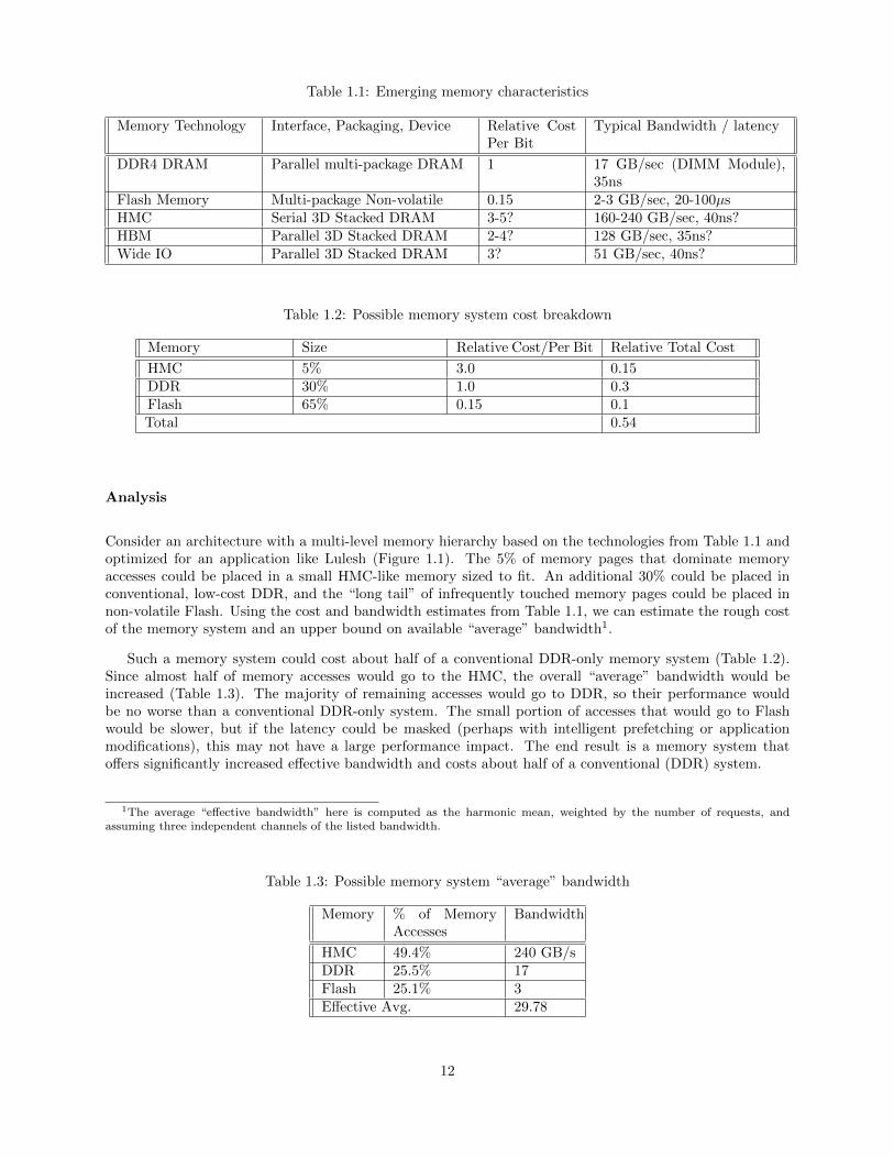
Table 1.1: Emerging memory characteristics

Memory Technology Interface, Packaging, Device Relative CostPer Bit

Typical Bandwidth / latency

DDR4 DRAM Parallel multi-package DRAM 1 17 GB/sec (DIMM Module),35ns

Flash Memory Multi-package Non-volatile 0.15 2-3 GB/sec, 20-100µsHMC Serial 3D Stacked DRAM 3-5? 160-240 GB/sec, 40ns?HBM Parallel 3D Stacked DRAM 2-4? 128 GB/sec, 35ns?Wide IO Parallel 3D Stacked DRAM 3? 51 GB/sec, 40ns?

Table 1.2: Possible memory system cost breakdown

Memory Size Relative Cost/Per Bit Relative Total Cost

HMC 5% 3.0 0.15DDR 30% 1.0 0.3Flash 65% 0.15 0.1Total 0.54

Analysis

Consider an architecture with a multi-level memory hierarchy based on the technologies from Table 1.1 andoptimized for an application like Lulesh (Figure 1.1). The 5% of memory pages that dominate memoryaccesses could be placed in a small HMC-like memory sized to fit. An additional 30% could be placed inconventional, low-cost DDR, and the “long tail” of infrequently touched memory pages could be placed innon-volatile Flash. Using the cost and bandwidth estimates from Table 1.1, we can estimate the rough costof the memory system and an upper bound on available “average” bandwidth1.

Such a memory system could cost about half of a conventional DDR-only memory system (Table 1.2).Since almost half of memory accesses would go to the HMC, the overall “average” bandwidth would beincreased (Table 1.3). The majority of remaining accesses would go to DDR, so their performance wouldbe no worse than a conventional DDR-only system. The small portion of accesses that would go to Flashwould be slower, but if the latency could be masked (perhaps with intelligent prefetching or applicationmodifications), this may not have a large performance impact. The end result is a memory system thatoffers significantly increased effective bandwidth and costs about half of a conventional (DDR) system.

1The average “effective bandwidth” here is computed as the harmonic mean, weighted by the number of requests, andassuming three independent channels of the listed bandwidth.

Table 1.3: Possible memory system “average” bandwidth

Memory % of MemoryAccesses

Bandwidth

HMC 49.4% 240 GB/sDDR 25.5% 17Flash 25.1% 3Effective Avg. 29.78

12

1.1.2 The Case Against...

Economics

The biggest potential pitfall for MLM is also economic. Used improperly, MLM has the potential to increasecost and decrease performance. Because some high-performance memory technologies (such as HMC) costmore than commodity DRAM, a memory system which relies too heavily on them will cost more than aconventional memory system. If that memory system is not managed properly, it may not be able to takeadvantage of the faster memory and will not justify the cost. Similarly, overuse of cheaper non-volatilememory may significantly degrade performance[8].

A related issue is that application diversity implies that no single mix of memory technologoies and sizeswill be optimal for all applications. As such, while a given MLM system might be cost-effective for someapplications, it may cost more and/or reduce performance for another set of applications. As such, onemust carefully consider the applications that will be running on the architecture, and potentially tune thoseapplications to the architecture, to ensure both performance and cost effectiveness.

Management

In addition to economics, a major impediment to successful deployment of MLM technology is its manage-ment. Software will need to be modified to place commonly used data in the fast “near” memory and lessfrequently used data in the “far” slow memory. Alternately, the operating system, runtime, or hardwarewill have to transparently move data from one memory level to the other by predicting future applicationrequirements.

All of these approaches have substantial costs. Modifying applications or runtimes requires programmereffort, insight, and will probably require a new generation of analysis tools. Adding hardware to manageMLM will incur substantial design costs as well as use additional chip area, increasing cost and possiblypower.

Latency

Finally, the simplistic bandwidth analysis presented in Section 1.1.1 only focuses on the bandwidth of newmemory technologies. This is insufficient because of the unusual latency characteristics these technologiespresent. For example, HMC-like memories offer dramatically higher bandwidth and throughput, but theirlatency is not much better than conventional DDR memory and can even be worse. Non-volatile memoriesoffer lower bandwidth, but also much higher latency (often by orders of magnitude). Additionally, the latencyof NV memories is often asymmetric2. Considering not only bandwidth but latency in data placement furthercomplicates MLM management. However, if data placement is not properly managed, the potential of MLMcan be squandered.

1.2 Three Paths to MLM Management

The memory characteristics of applications of interest to the DOE vary considerably. Figure 1.1 shows thenumber of post-cache references to different 4K memory pages across three applications. Even this small setexhibits substantial diversity. MiniAero (leftmost graph) shows a small number of well defined regions whichare highly accessed. Lulesh shows a large number of regions. RSBench (rightmost) has a very irregularaccess pattern without well defined regions.

2Different read and write latencies.

13

!! !Figure 1.1: Address histograms sorted by address

Because of this application diversity and the trade-offs inherent in different management policies, webelieve there is no “One Size Fits All” solution for managing MLM systems. Thus, we explore three paths:Algorithmic, Manual, and Automatic Management.

1.2.1 Algorithmic

Algorithmic management of MLM requires restructuring and rewriting the fundamental algorithms and/ordata structures of a code to take advantage of multiple levels of memory. Algorithmic management requiresa high level of programmer effort, but has a high potential to improve performance. A disadvantage ofthe algorithmic approach is that it may require rewrites of applications whenever new levels of memory areadded. Additionally, multi-physics applications that contain several algorithms (often contained in separatelibraries) may be difficult to adapt to this approach. However, it may be possible for algorithmic restructuringto be combined with other approaches to provide “hints” to the runtime or hardware about data placement.

A detailed analysis of algorithmic restructuring is beyond the scope of this document. However, anapplication of this approach can be found in a previous paper[1].

1.2.2 Manual

Manual management of MLM requires the programmer to identify blocks of application memory (usuallymalloc() allocations) which should be stored in a given level of memory. This approach is less invasivethan algorithmic restructuring, but does require substantial programmer effort to identify and “tag” criticalmemory regions for placement in fast memory.

An interesting aspect of manual management is that programmer intuition about which memory regionsare most critical is often incorrect. Many frequently accessed data structures are are simply moved intothe system’s SRAM caches3 and benefit minimally from being placed in faster memory. For example, athread’s stack is accessed very frequently, but produces very few cache misses to main memory. Instead,higher performance is achieved by identifying regions which are accessed frequently, but not too frequently.To accomplish this, new program analysis tools will need to be produced.

Chapter 4 covers manual MLM management and introduces MemSieve (Section 4.2), an analysis tool toaid in identifying memory critical regions of an application.

3e.g. L1 or L2 cache

14

1.2.3 Automatic

Automatic management of MLM requires specialized hardware which tracks main memory accesses and co-ordinates movement of data between different layers of memory. This approach has the benefit of minimizingprogrammer effort, but does require extra hardware. This hardware requires tables to track accesses, DMAengines to transfer between layers, and a TLB-like structure to determine in which memory level a givenaddress resides. Together, these structures could be power- and area-hungry, increasing cost.

An interesting finding of our analysis of automatic management policies is that they differ from conven-tional caching policies. Specifically, most cache policies focus on replacement – deciding what to removefrom a cache when you need to add data to it. In contrast, MLM is much more sensitive to addition policies– deciding if it is worth bringing something into the “fast” memory when it is accessed. This is because thelatency of “fast” memory is so similar to that of conventional DDR DRAM.

Chapter 5 explores automatic management.

1.3 Roadmap

Chapter 2 discusses the methodology used in experiments in this report. Chapter 3 discusses a designspace exploration of HMC different configurations. Chapter 4 covers manual MLM management approaches.Chapter 5 covers automatic MLM management approaches. Finally, Chapter 6 presents conclusions andfuture work.

15

16

Chapter 2

Methodology

In this chapter we present our experimental methodology. As mentioned in the previous chapter, we analyzethe performance of ASC codes at the node level on a two-level memory system with near HMC and far DDR.Because the hardware and software infrastructures do not yet exist for the architectures and managementstrategies we are evaluating, we primarily employ simulation. However, we do use real hardware when avail-able to validate simulation results. In Section 2.1 we present the applications studied and in Section 2.2 wedescribe our simulation infrastructure including simulation validation studies and how we enabled simulationat scale. Finally, we present the two architectures used throughout our studies in Section 2.2.2.

2.1 Applications

A major call in this milestone was to analyze the impact of MLM on key kernels and algorithms found inASC codes. To that end, we selected four mini-apps from the APEX benchmark suite. This suite is designedto be used by vendors and labs to evaluate proposed systems for the 2020 Crossroads/NERSC procurement.As such, the mini-apps cover a wide variety of algorithms used across multiple labs. By studying theseapplications, we hope to gain insight that can be used to steer procurement decisions, enable meaningfulinteraction with vendors about future architectures, as well as assist application developers in effectively usingsystems with MLM. For this milestone, we selected four applications, MiniPIC, PENNANT, HPCG, andSNAP. Additionally, to increase confidence that our results translated to real systems, we opted to simulatethese applications at larger scales than have previously been attempted. In this study each benchmark issized to yield a data footprint of 1GB to 8GB, depending on the particular experiment. Simulating at thisscale required a number of simulator improvements (Section 2.2) as well as a sampling methodology whichwe will discuss in the following subsection. The input parameters and memory usage for each application isshown in Table 2.1. A brief description of each mini-app is provided below.

MiniPIC [2] uses the particle-in-cell (PIC) method to solve the discrete Boltzman equation in an electro-static field in an arbitrary domain with reflective walls. It solves this equation using the following algorithmon an unstructured mesh. Particles are weighted to the grid as a charge density and Poisson’s equation issolved. The electric field is then calculated and weighted to the particle locations. Finally, the particlesare accelerated and moved to new locations. As particles interact with each other and walls, new particlesmay be created. This process is repeated in each time step. MiniPIC uses the Trilinos Tpetra library formatrix and vector operations. For scalability at a high level, MiniPIC spreads the field over MPI ranks; oncea particle cannot move any farther in its rank, it moves to a neighboring one. For node-level parallelism,MiniPIC employs threading via the Trilinos Kokkos package. Kokkos enables performance portability byallowing users to select architecture-specific threading models (e.g., CUDA or OpenMP). In this study weuse the OpenMP backend and do not use MPI. MiniPIC was developed at Sandia National Laboratories.

PENNANT [5] is a hydrodynamics algorithm which uses Lagrangian and staggered-grid methods. Thealgorithm is implemented over a 2D unstructured finite-volume mesh. For parallelism, PENNANT doesgeometric domain decomposition across MPI ranks and, at the node level, employs OpenMP threads todivide the local mesh into (almost) independent computational chunks. PENNANT was developed by LosAlamos National Laboratory. During our analysis we identified that PENNANT has a significant number of

17

Table 2.1: Application parameters

Application Version Input Memory Parameters

MiniPIC APEX releaseon 2/26/16

big 8G Nx=Ny=Nz=7; --dt=0.5 --tfinal=2.0

--nparts=8000

MiniPIC APEX releaseon 2/26/16

small 1.8G Nx=Ny=Nz=4; --dt=0.5 --tfinal=2.0

--nparts=8000

PENNANT 0.9 big 8G leblancbigx6 (same as default leblancbigx4 with’meshparams 960 8640 1.0 9.0’ and ’dtinit 1.67e-4’

PENNANT 0.9 small 1G leblancbigx6 (same as default leblancbigx4 with’meshparams 320 2880 1.0 9.0’ and ’dtinit 5.e-4’

HPCG 3.0 big 8G nx=272, ny=272, nz=136HPCG 3.0 medium 4G nx=192, ny=192, nz=136HPCG 3.0 small 1G nx=112, ny=112, nz=112SNAP 1.06 big 8G APEX ’in s’ input modified with npey=1, npez=1,

nx=128, ny=16, nz=20, ichunk=16SNAP 1.06 small 1G APEX ’in s’ input modified with npey=1, npez=1,

nx=32, ny=12, nz=16, ichunk=16MiniFE 2.0 small 11M -nx 30 -ny 30 -nz 30

Lammps 2/16/16 re-lease

small 25M -i in.eam -sf omp

Lulesh 2.0.3 small 10M -s 20 -i 10 -r 11

CoMD 1.1 small 19.5M --nx 25 --ny 20 --nz 20 --nSteps 5

small allocations (shown later in this report). Although we have not modified the code for the remainder ofthis study, in part to ensure we analyze the existing code, the use of an optimized allocator or memory poolscheme could significantly improve the performance of PENNANT on some architectures.

HPCG [4] is an open-source benchmark that was developed as an alternative method to High Per-formance LINPACK (HPL) for ranking HPC systems. HPCG does a fixed number of conjugate gradientiterations using a simple multigrid preconditioner. Like the previous applications, HPCG uses both MPI andOpenMP parallelism. In particular, OpenMP parallel for loops are used for many of the vector and matrixoperations. Additionally the SpMV algorithm is threaded over matrix rows.

SNAP [18] is representative of discrete ordinate neutral particle transport applications. Although itimplements no ’real’ physics, SNAP was developed to mimic the computational workload, data layout,memory usage, and communication patterns found in real applications. SNAP executes a number of timestepswhich are structured in a two level nested loop. At each timestep, the outer loop executes until either aset number of iterations have been executed or convergence is reached. Likewise, within each outer loopiteration, an inner loop is executed until a set number of inner iterations have been executed or convergenceis reached. The majority of computation occurs within inner loop iterations, however outer iterations docompute an outer source sum as well as check for convergence. SNAP uses both MPI and OpenMP forparallelism. At the node-level, OpenMP parallel loops are used for the convergence testing functions, to suminner and outer sources, SNAP was developed by Los Alamos National Laboratory.

In addition to the above mini-apps, we also used a number of other applications for early design spaceexploration studies and some validation work. Unlike the previous applications, we do not execute theseapplications at scale, enabling us to quickly prune the design space. For validation in particular, we used theSTREAM benchmark which exercises system bandwidth. For early analysis studies, we used Lammps[13, 14],a molecular dynamics application; MiniFE[6], an unstructured implicit finite element code; Lulesh[10], ahydrodynamics code; and CoMD[6], a molecular dynamics application. Each application was executed with16 threads. Additional parameters and the memory footprint is listed in Table 2.1. These latter mini-appswere selected because they exhibit a diverse set of main memory access patterns[8]. MiniFE has a small

18

number of memory regions (contiguous pages) with similar access characteristics and a low Gini coefficient,indicating a relatively equal number of accesses per page. Lulesh has multiple different regions and a highGini coefficient, indicating a small set of pages that are accessed disproportionately. CoMD and Lammpshave more irregular access patterns.

2.1.1 Methodology for Simulating at Scale

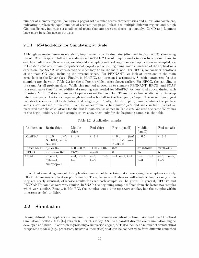
Although we made numerous scalability improvements to the simulator (discussed in Section 2.2), simulatingthe APEX mini-apps in full at the scales shown in Table 2.1 would require weeks to months or more. Thus, toenable simulation at those scales, we adopted a sampling methodology. For each application we sampled oneto two iterations of the main computational loop at each of the beginning, middle, and end of the application’sexecution. For SNAP, we considered the inner loop to be the main loop. For HPCG, we consider iterationsof the main CG loop, including the preconditioner. For PENNANT, we look at iterations of the mainevent loop in the Driver class. Finally, in MiniPIC, an iteration is a timestep. Specific parameters for thissampling are shown in Table 2.2 for the different problem sizes shown earlier. For HPCG, the sampling isthe same for all problem sizes. While this method allowed us to simulate PENNANT, HPCG, and SNAPin a reasonable time frame, additional sampling was needed for MiniPIC. As described above, during eachtimestep, MiniPIC does a number of operations on the particles. Therefore we further divided a timestepinto three parts. Particle charge weighting and solve fall in the first part, charge. The second part, fieldincludes the electric field calculation and weighting. Finally, the third part, move, contains the particleacceleration and move functions. Even so, we were unable to simulate field and move in full. Instead wemeasured over the calculations for the first N particles, as shown in Table 2.2. We used the same ’N’ valuesin the begin, middle, and end samples so we show them only for the beginning sample in the table.

Table 2.2: Application samples

Application Begin (big) Middle(big)

End (big) Begin (small) Middle(small)

End (small)

MiniPIC t=0.0; fieldN=10M; moveN=5000

t=0.5 t=1.5 t=0.0; fieldN=1.5M; moveN=300K

t=0.5 t=1.5

PENNANT cycles 0-2 5000-5002 11100-11102 0-2 3700-3702 7470-7472HPCG iterations 0-1 24-25 49-50 0 25 50SNAP inner=1,

outer=1,timestep=1

i=4, o=4,t=3

i=3, o=5,t=8

i=1, o=1, t=1 i=4, o=4,t=3

i=3, o=5,t=8

Without simulating more of the application, we cannot be certain that an averaging the samples accuratelyreflects the average application performance. Therefore in our studies we will combine samples only whenthey are nearly identical, otherwise results for each each sample will be given. In general, HPCG’s andPENNANT’s samples were very similar. In SNAP, the beginning sample differed from the latter two sampleswhich were similar. Finally, in MiniPIC, the samples across timesteps were similar, but the samples withintimesteps tended to differ.

2.2 Simulation

Having defined the applications, we now discuss our simulation infrastructure. We used the StructuralSimulation Toolkit (SST) [15] version 6.0 for this study. SST is a parallel discrete event simulation enginedeveloped at Sandia. In addition to providing a simulation engine, SST also includes a number of architecturalcomponent models (e.g., processors, networks, memories) that can be connected to form different simulated

19

DRAML3Cache

L3Cache

Network Directory MemoryController

Core L2L1

Core L2L1

Figure 2.1: Generic SST configuration

Application

Ariel Pintool

Mem

L3Ariel CPUC

C

…

L1/L2

L1/L2

Mem

L3

NoC

Figure 2.2: An SST configuration with Ariel, MemHierarchy, and Merlin

system architectures. An example of how an architecture might be constructed from individual componentsis shown in Figure 2.1. We describe the components used in this study below.

We used the Ariel processor model for our multicore processor. Ariel consists of two parts that interactvia a shared memory region. The first is a PIN tool that utilizes Intel’s PIN framework [11] to instrument anative binary. As the binary runs on the host processor, Ariel’s PIN tool intercepts memory instructions andpasses them to the second part, the simulated processor. The simulated processor implements multiple cores,one per thread. It also models a page table manager which manages memory allocation and deallocationas well as virtual-to-physical address translation. The queue between the simulated processor and the PIN-instrumented binary enables the simulation to stall the binary execution when it runs too far ahead of thesimulation. As such, Ariel allows the use of native binaries, is fairly lightweight, and accurately modelsmemory system traffic although it does not model the full execution pipeline and functional units. Toapproximate computation, Ariel uses no-ops when there are no memory instructions to execute (i.e., theapplication is tied up in computation). Figure 2.2 illustrates how Ariel fits into the larger simulation.

MemHierarchy is a collection of memory component models including caches, buses, directory controllers,and memory controllers. MemHierarchy is a cycle-level model that provides highly flexible cache topologieswith directory-based coherence (MSI and MESI). In addition to these components, MemHierarchy imple-ments memory controller interfaces, called memory backends, to a number of memory simulators. To modelthe DDR in this study, we used the DRAMSim simulator developed at University of Maryland. To modelHMC, we used Texas Tech’s Goblin HMC simulator and VaultSim, a generic vaulted memory componentprovided by SST.

For the on-chip network (NoC) model, we used SST’s Merlin component. Merlin is an flexible, cycle-level network simulator that can be used to model large scale intra-node and off-chip networks as well asthe smaller on-chip networks needed for our single node studies. Merlin can implement arbitrary networktopologies and models traffic at the flit level.

In the following section we describe the scalability, performance, and functional improvements that werenecessary for simulating MLM at the scales presented in the previous section. We then discuss the twoarchitectures we considered along with their simulation parameters. Finally we present the results of somevalidation studies.

20

2.2.1 Simulation Improvements

To enable scalable simulation, we made a number of improvements to the Ariel and MemHierarchy compo-nents. To reduce execution overhead, we re-wrote the MemHierarchy caches, directory, and memory NIC tobe primarily event driven instead of clock driven. While clocks are still used, they are deactivated unlessevents need to be handled. This change reduced run time by approximately 30% for the STREAM bench-mark. The second major improvement involved streamlining and reorganizing code in both MemHierarchyand Ariel to eliminate unnecessary compute. We found that these changes reduced runtime by a further5-15% (depending on the change). Additionally, to reduce the memory overhead, we added the option tosimulate without backing the memory system (i.e., tracking memory values at the memory). For simulationswith Ariel where simulated data values do not affect the application execution, we can reduce the footprintfrom the size of the simulated memories (e.g., 10s of GBs) to one GB or less. All of these improvementswere incorporated into the SST 6.0 release.

In response to the validation studies described next, we also made some simulated performance improve-ments. This included support for fine-grained address striping across memories, eliminating a bottleneck atthe memory NIC which handles address to destination translation, and improved control over throughputat the memory controller. We also fixed a number of performance bugs that had not been seen at smallersimulation scales. One significant bug was that the cache set index calculation at cache arrays was notdistributed-cache aware leading to unused cache sets. In turn, depending on the number of cache sets andthe number of distributed cache slices in a system, the distributed cache capacity was effectively lowered.Fixing these bugs and adding the additional capabilities allowed us to realistically model real architectures.

Finally, to support multi-level memory, we added a number of capabilities in Ariel to allow applicationsto manage the memory. We extended the Ariel API which provides applications with ‘hooks’ to control andinteract with the simulation (e.g., start the simulation, trigger a statistics dump, get the simulated time,etc.) with operations for allocating memory in specific memory pools. While multi-level memory refers toseparate memory types as “levels”, Ariel operates with the concept of memory “pools”. Each pool can betargeted at a separate memory and the new API calls allow the application to allocate and free memorydirectly in particular pools as well as to flag that upcoming mallocs should be allocated to a specific pool.

2.2.2 Architectures

As mentioned in the introduction, to determine whether applications responded similarly to the presence ofmulti-level memory independent of the architecture, we studied two architectures with completely differentnetwork topologies, processor capabilities, and memory hierarchies. Each architecture reflects a prevailingdesign strategy found in real hardware. The first, heavyweight architecture, has a few (i.e., 8-16) large,powerful cores connected to a deep cache hierarchy. Many traditional architectures, such as the Intel Xeon,IBM Power, and AMD Opteron fall in this category. The second architecture, lightweight features manyless powerful cores with a shallower cache hierarchy. An example of this kind of architecture would be theIntel Xeon Phi. Heavyweight architectures tend to maximize single-thread performance while lightweightarchitectures are designed for high throughput. The specific architectures studied here are shown in Fig-ure 2.3. The simulation parameters are given in Table 2.3. Note that the purpose of studying these twoarchitectures is not to determine which of the two paths is better. Rather we seek to determine how differentarchitectures affect applications’ memory access patterns and ability to use multi-level memory. Accordingly,we do not attempt to equalize the available memory bandwidth in the systems or otherwise single out theeffect of particular architectural features. In terms of real hardware, the lightweight model resembles anIntel Knights Landing (Xeon Phi) while the heavyweight model is similar to the Intel Sandy Bridge (Xeon)architecture.

21

L3Core

Mem

Core

L3

Core

Core

CoreCore

Core

Core

L3

L3

L3

L3

L3

L3

Mem

Mem

Mem

Core

L1

L2

(a) Heavyweight architecture

TileHMCDDR

C CL1 L1L2

(b) Lightweight architecture

Figure 2.3: Architectures studied

Table 2.3: Simulation parameters

Architecture Component Parameters

Heavyweight

Processor 8 cores, 2.66GHz, 3 reqs/cycleCaches Private 32KB L1 (8-way assoc, 4 cycles), Private 256KB L2 (8-way assoc, 6

cycles), Shared distributed L3 with 8 2MB slices (16-way assoc, 12 cycles),MESI

Memory 2 HMC @ 160GB/s, 2 DDR @ 20GB/s, capacities vary by experimentNetwork Ring (merlin.torus), 96GB/s, 300ps link latency

Lightweight

Processor 72 cores, 1.4GHz, 2 reqs/cycleCaches Private 32KB L1 (8-way assoc, 2 cycles), 512KB L2 cache shared between

2 cores (16-way assoc, 6 cycles), MESIMemory 8 HMC @ 160GB/s, 6 DDR @ 20GB/s, capacities vary by experimentNetwork 8x8 mesh, 57GB/s, 50ps link latency

2.2.3 Validation

To validate our simulation models, we performed two studies. The first study validated that the GoblinHMC simulator’s bandwidth characteristics matched that of real HMC hardware. The second validated thatfor the STREAM benchmark we could attain similar bandwidth on a simulated Sandy Bridge architectureand a real Sandy Bridge chip. Additionally, near the end of this study, early Knight’s Landing (Xeon Phi)hardware became available. While we do not rigorously validate our lightweight architecture against it, inpart because the software environment for the Xeon Phi (Knights Landing) is still rapidly changing, we willpresent some comparisons throughout the study.

To validate the Goblin HMC simulation model, we ran a number of access patterns through our PicoEX800 HMC testbed. This testbed features a 2GB HMC connected to four Stratix V FPGAs (one perlink). The access patterns were chosen to exercise a variety of contention patterns. Each pattern generatesrandom accesses from a specific link to a specific portion of the HMC (e.g., quad, vault, or bank). Figure 2.4illustrates the patterns. In the top row, links access the colored region in their local quad. In the bottomrow, all links access the same colored region. The normalized bandwidth measurements from these accesspatterns are shown in Figure 2.5 in red. Measurements are normalized to the bandwidth of accessing randomaddresses in the link’s local quad (“own quad”). The next bar shows the original GoblinHMC simulator.While the simulated bandwidth matches the same trend as the measured bandwidth for access patternsat the quad and bank level, the vault patterns (‘own vault’ and ‘same vault’) differ significantly from themeasured pattern. In response to this validation study, a change was made to the simulated vault controller’scontention management which resulted in the tan bar in the figure. Although the absolute numbers stillvary in a few cases, the hardware and simulated trends now match.

22

Quad Vault Bank

Own bank

Same bank

Own vault

Same vault

Own quad

Same quad

Figure 2.4: Studied access patterns: links access areas of their local quads (top) and links access the samearea in a single quad (bottom)

0

0.2

0.4

0.6

0.8

1

1.2

Allquads Ownquad Ownvault Ownbank Samequad Samevault Samebank

Band

widthnormalizedto

"Ownqu

ad"

AccessPattern

HMChardware GoblinHMC- original GoblinHMC- bugfix

Figure 2.5: GoblinHMC validation study

23

0

10

20

30

40

50

60

1 2 3 4 5 6 7 8 9 10Ba

ndwidth(G

B/s)

Arraysize(in100Kelements)

Hardware OriginalW/throughputfix W/512BstripingW/64Bstriping

Figure 2.6: Sandy Bridge socket validation study

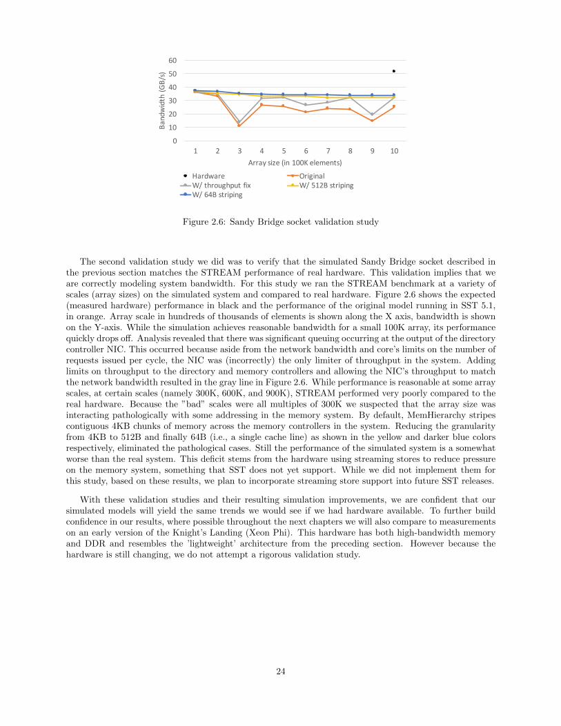
The second validation study we did was to verify that the simulated Sandy Bridge socket described inthe previous section matches the STREAM performance of real hardware. This validation implies that weare correctly modeling system bandwidth. For this study we ran the STREAM benchmark at a variety ofscales (array sizes) on the simulated system and compared to real hardware. Figure 2.6 shows the expected(measured hardware) performance in black and the performance of the original model running in SST 5.1,in orange. Array scale in hundreds of thousands of elements is shown along the X axis, bandwidth is shownon the Y-axis. While the simulation achieves reasonable bandwidth for a small 100K array, its performancequickly drops off. Analysis revealed that there was significant queuing occurring at the output of the directorycontroller NIC. This occurred because aside from the network bandwidth and core’s limits on the number ofrequests issued per cycle, the NIC was (incorrectly) the only limiter of throughput in the system. Addinglimits on throughput to the directory and memory controllers and allowing the NIC’s throughput to matchthe network bandwidth resulted in the gray line in Figure 2.6. While performance is reasonable at some arrayscales, at certain scales (namely 300K, 600K, and 900K), STREAM performed very poorly compared to thereal hardware. Because the ”bad” scales were all multiples of 300K we suspected that the array size wasinteracting pathologically with some addressing in the memory system. By default, MemHierarchy stripescontiguous 4KB chunks of memory across the memory controllers in the system. Reducing the granularityfrom 4KB to 512B and finally 64B (i.e., a single cache line) as shown in the yellow and darker blue colorsrespectively, eliminated the pathological cases. Still the performance of the simulated system is a somewhatworse than the real system. This deficit stems from the hardware using streaming stores to reduce pressureon the memory system, something that SST does not yet support. While we did not implement them forthis study, based on these results, we plan to incorporate streaming store support into future SST releases.

With these validation studies and their resulting simulation improvements, we are confident that oursimulated models will yield the same trends we would see if we had hardware available. To further buildconfidence in our results, where possible throughout the next chapters we will also compare to measurementson an early version of the Knight’s Landing (Xeon Phi). This hardware has both high-bandwidth memoryand DDR and resembles the ’lightweight’ architecture from the preceding section. However because thehardware is still changing, we do not attempt a rigorous validation study.

24

Chapter 3

Design Space Exploration

Before analyzing multi-level memory management in the following sections, we look at the design spacefor the HMC memory. We begin by analyzing the potential performance improvements when moving fromtraditional DDR DRAM to the higher bandwidth HMC.

3.1 Potential Performance with HMC

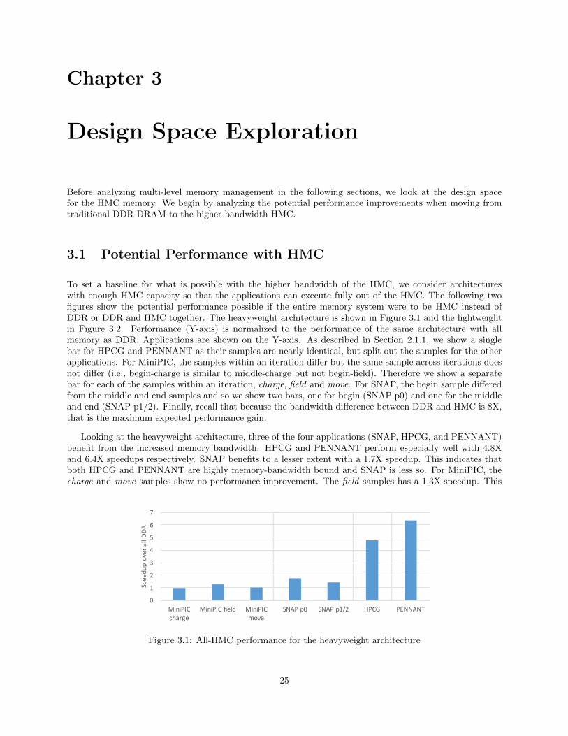
To set a baseline for what is possible with the higher bandwidth of the HMC, we consider architectureswith enough HMC capacity so that the applications can execute fully out of the HMC. The following twofigures show the potential performance possible if the entire memory system were to be HMC instead ofDDR or DDR and HMC together. The heavyweight architecture is shown in Figure 3.1 and the lightweightin Figure 3.2. Performance (Y-axis) is normalized to the performance of the same architecture with allmemory as DDR. Applications are shown on the Y-axis. As described in Section 2.1.1, we show a singlebar for HPCG and PENNANT as their samples are nearly identical, but split out the samples for the otherapplications. For MiniPIC, the samples within an iteration differ but the same sample across iterations doesnot differ (i.e., begin-charge is similar to middle-charge but not begin-field). Therefore we show a separatebar for each of the samples within an iteration, charge, field and move. For SNAP, the begin sample differedfrom the middle and end samples and so we show two bars, one for begin (SNAP p0) and one for the middleand end (SNAP p1/2). Finally, recall that because the bandwidth difference between DDR and HMC is 8X,that is the maximum expected performance gain.

Looking at the heavyweight architecture, three of the four applications (SNAP, HPCG, and PENNANT)benefit from the increased memory bandwidth. HPCG and PENNANT perform especially well with 4.8Xand 6.4X speedups respectively. SNAP benefits to a lesser extent with a 1.7X speedup. This indicates thatboth HPCG and PENNANT are highly memory-bandwidth bound and SNAP is less so. For MiniPIC, thecharge and move samples show no performance improvement. The field samples has a 1.3X speedup. This

0

1

2

3

4

5

6

7

MiniPICcharge

MiniPICfield MiniPICmove

SNAPp0 SNAPp1/2 HPCG PENNANT

SpeedupoverallDD

R

Figure 3.1: All-HMC performance for the heavyweight architecture

25

0

1

2

3

4

5

6

MiniPICcharge

MiniPICfield MiniPICmove

SNAPp0 SNAPp1 HPCG PENNANT

SpeedupoverallDD

R

Figure 3.2: All-HMC performance for the lightweight architecture

occurs because on the HMC model, MiniPIC varies for this sample. In some executions it achieves just a1.0X to 1.05X improvement, while in others it achieves nearly a 1.7X improvement. We have not confirmedthe reason for this variance but believe it is tied to the order that particles are processed (i.e., insertedonto the particle list). An algorithmic change to ensure a “good” ordering might ensure that this phase ofexecution always performs well. However, the improvement may not benefit the application as a whole asthe move phase dominates execution time.

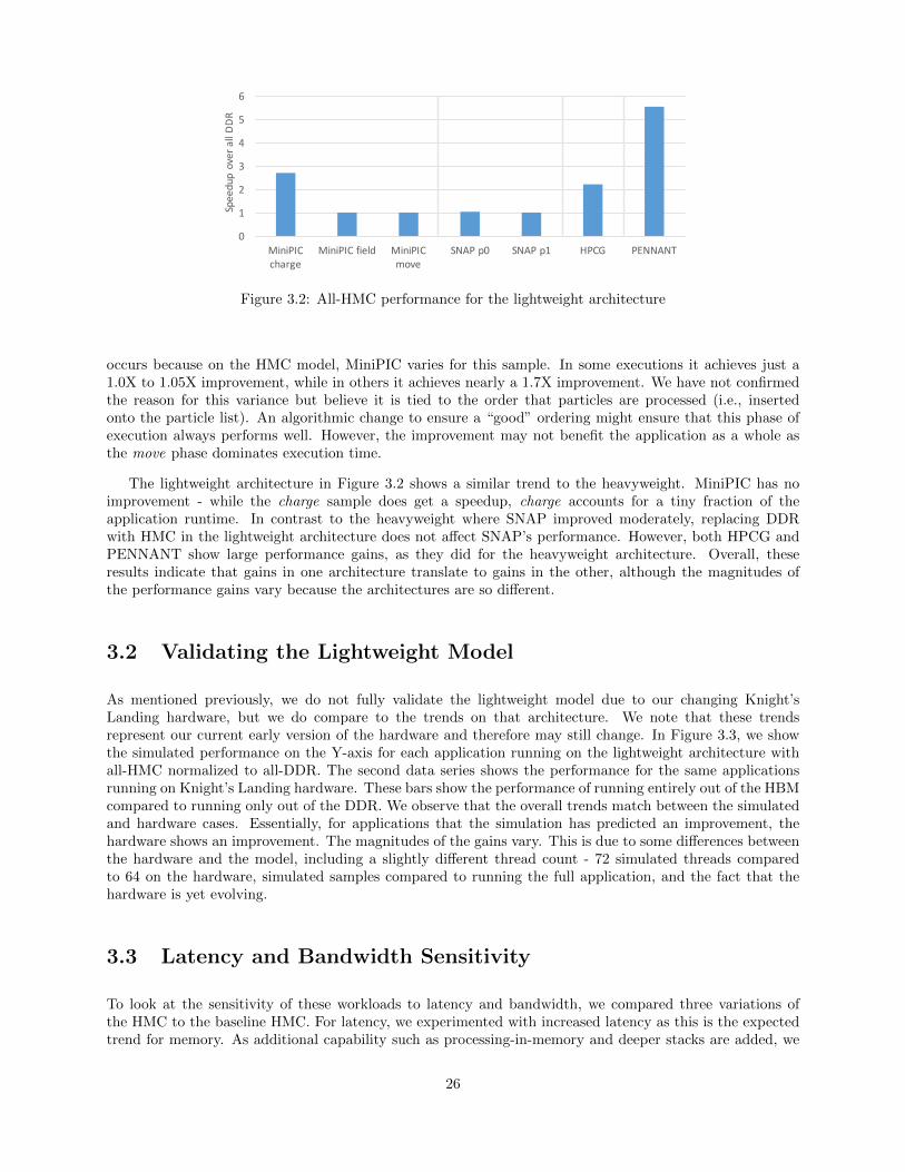
The lightweight architecture in Figure 3.2 shows a similar trend to the heavyweight. MiniPIC has noimprovement - while the charge sample does get a speedup, charge accounts for a tiny fraction of theapplication runtime. In contrast to the heavyweight where SNAP improved moderately, replacing DDRwith HMC in the lightweight architecture does not affect SNAP’s performance. However, both HPCG andPENNANT show large performance gains, as they did for the heavyweight architecture. Overall, theseresults indicate that gains in one architecture translate to gains in the other, although the magnitudes ofthe performance gains vary because the architectures are so different.

3.2 Validating the Lightweight Model

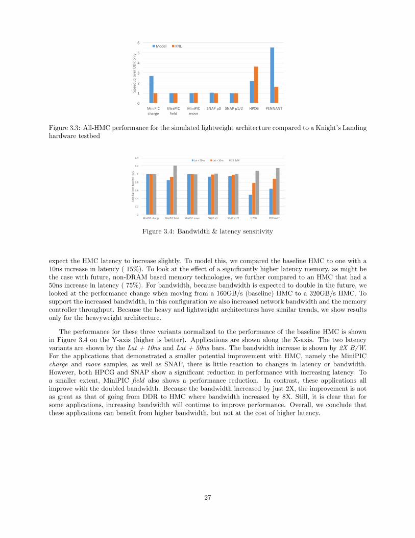
As mentioned previously, we do not fully validate the lightweight model due to our changing Knight’sLanding hardware, but we do compare to the trends on that architecture. We note that these trendsrepresent our current early version of the hardware and therefore may still change. In Figure 3.3, we showthe simulated performance on the Y-axis for each application running on the lightweight architecture withall-HMC normalized to all-DDR. The second data series shows the performance for the same applicationsrunning on Knight’s Landing hardware. These bars show the performance of running entirely out of the HBMcompared to running only out of the DDR. We observe that the overall trends match between the simulatedand hardware cases. Essentially, for applications that the simulation has predicted an improvement, thehardware shows an improvement. The magnitudes of the gains vary. This is due to some differences betweenthe hardware and the model, including a slightly different thread count - 72 simulated threads comparedto 64 on the hardware, simulated samples compared to running the full application, and the fact that thehardware is yet evolving.

3.3 Latency and Bandwidth Sensitivity

To look at the sensitivity of these workloads to latency and bandwidth, we compared three variations ofthe HMC to the baseline HMC. For latency, we experimented with increased latency as this is the expectedtrend for memory. As additional capability such as processing-in-memory and deeper stacks are added, we

26

0

1

2

3

4

5

6

MiniPICcharge

MiniPICfield

MiniPICmove

SNAPp0 SNAPp1/2 HPCG PENNANT

SpeedupoverDDR

only

Model KNL

Figure 3.3: All-HMC performance for the simulated lightweight architecture compared to a Knight’s Landinghardware testbed

0

0.2

0.4

0.6

0.8

1

1.2

1.4

MiniPICcharge MiniPICfield MiniPICmove SNAPp0 SNAPp1/2 HPCG PENNANT

SpeedupoverbaselineHM

C

Lat+50ns Lat+10ns 2XB/W

Figure 3.4: Bandwidth & latency sensitivity

expect the HMC latency to increase slightly. To model this, we compared the baseline HMC to one with a10ns increase in latency ( 15%). To look at the effect of a significantly higher latency memory, as might bethe case with future, non-DRAM based memory technologies, we further compared to an HMC that had a50ns increase in latency ( 75%). For bandwidth, because bandwidth is expected to double in the future, welooked at the performance change when moving from a 160GB/s (baseline) HMC to a 320GB/s HMC. Tosupport the increased bandwidth, in this configuration we also increased network bandwidth and the memorycontroller throughput. Because the heavy and lightweight architectures have similar trends, we show resultsonly for the heavyweight architecture.

The performance for these three variants normalized to the performance of the baseline HMC is shownin Figure 3.4 on the Y-axis (higher is better). Applications are shown along the X-axis. The two latencyvariants are shown by the Lat + 10ns and Lat + 50ns bars. The bandwidth increase is shown by 2X B/W.For the applications that demonstrated a smaller potential improvement with HMC, namely the MiniPICcharge and move samples, as well as SNAP, there is little reaction to changes in latency or bandwidth.However, both HPCG and SNAP show a significant reduction in performance with increasing latency. Toa smaller extent, MiniPIC field also shows a performance reduction. In contrast, these applications allimprove with the doubled bandwidth. Because the bandwidth increased by just 2X, the improvement is notas great as that of going from DDR to HMC where bandwidth increased by 8X. Still, it is clear that forsome applications, increasing bandwidth will continue to improve performance. Overall, we conclude thatthese applications can benefit from higher bandwidth, but not at the cost of higher latency.

27

28

Chapter 4

Manual Management

4.1 Software Approaches & Trade-offs

In this section we evaluate methods for managing multi-level memory (MLM) in software. As mentionedin Chapter 1, software management is attractive because it has the potential to be very efficient (albeitwith significant manual effort) and because it does not rely on hardware vendors for its implementation.We describe three major strategies for such management. In algorithmic, an application writer employsdifferent data structures and algorithms to align the application’s memory behavior to the target memorytechnology. For example, the writer might restructure the code so that a section of code can operatecompletely out of high-bandwidth memory and make use of the increased memory bandwidth. Because ofthe demand on programmers, as well as the need for algorithm-specific optimizations, we don’t explore thisconcept deeply here. Still, in the following analysis, we will make note of areas where code changes mightcomplement the other management techniques. A second strategy is to utilize OS or runtime managedMLM. In this technique, the OS determines where to allocate memory and may even migrate that memorybetween memory levels if needed. A simple OS approach might be application-unaware while more complexmanagers might monitor the application and memory performance to inform the management. Finally,the third management strategy, manual, requires that the application manage its own memory. Manualmanagement generally requires code changes to specify where data should be allocated, as well as to migratedata between memory levels if necessary. Note that OS/runtime management and application managementare not mutually exclusive. One can imagine systems where some memory is handled by each, as well assystems where the OS manages the MLM in consultation with the application.

We focus on these last two, OS and application management. In addition to these primary methods, weevaluate whether these decisions can be made statically for a run versus dynamically throughout the executionof the application. In static allocation, the OS or application writer would make its allocation decisions onceand they would remain for the entirety of the execution. The advantage of static is its simplicity - no re-evaluating mapping decisions and no re-mapping and its accompanying latency and bandwidth overheads.However static allocation has the downside of likely not being sufficient for applications which have distinctphases where different memory regions are touched. The second variable is whether allocation is done at apage or malloc granularity. This variable does not apply to application-managed MLM as applications donot use the concept of pages and therefore can only operate at the malloc level. For the OS however, thereare trade-offs. In general, large pages and mallocs have a higher probability of containing both bandwidth-bound and bandwidth-insensitive regions. Putting either in an HMC wastes space that could otherwise begiven to only bandwidth-bound pages or allocations. Further, with very large allocations, one may not beable to pack mallocs into the HMC and use the entire available memory.

In the following subsection we look deeper at the programmer effort, the expected performance, and thepotential overhead involved in both OS/runtime-managed MLM and manual/programmer managed MLM.In Section 4.2 we present MemSieve, an analysis tool we developed to analyze an application’s memory use.Finally, in Section 4.3 we compare the performance of the manual approaches, including static and dynamicallocation and malloc versus page-based allocation granularity.

29

4.1.1 Trade-offs

Application- and OS-managed MLM trade-off programmer effort for potential performance. We summarizethe key advantages and disadvantages of each management method (OS and application) in Table 4.1. OS-management has the advantage of requiring little to no effort from the programmer. For legacy applicationsthis is attractive. On the other hand, the OS has no knowledge of the program behavior and so musteither blindly guess where to allocate memory or must use potentially high-overhead runtime profiling tointelligently steer its decisions. Such profiling is complicated by the OS’s lack of visibility into memoryusage. Unless there is a TLB-miss the OS is not involved in memory accesses. Further, even if the OS weremonitoring accesses, the OS does not differentiate between accesses that hit in a cache versus those that goall the way out to memory. This distinction is important as many frequently-accessed regions of memoryend up being cache resident and so do not use main memory bandwidth.

Table 4.1: Trade-offs in management approaches

OS/Runtime Application

+ Able to capture allocations not under applicationcontrol

+ Knowledge of program behavior for better allocation

+ No intervention from programmer required + Application analysis to determine memory behaviorcan be done offline

- No program knowledge for smart allocation - No standard way to manage allocation within localarrays or library calls

- Intelligent allocation requires programmer assistanceor runtime profiling

- Pervasive code changes

- Increased page-table complexity - Offline analysis may be difficult if memory use varieswidely with input

- Potentially expensive re-mapping to support dy-namic

- Potentially need to repeat offline analysis every timethere’s a new architecture

In contrast to OS-management, application-managed MLM also incurs overhead but most is offline. Theapplication writer must spend time profiling the application to determine how it uses memory, as memoryuse is not always obvious (e.g., many frequently used allocations end up in cache). The writer must then editthe application to explicitly manage memory, including moving and copying allocations if dynamic migrationis needed.

If the application requires dynamic migration, further support must be added to the application tomove allocations between memories throughout execution. Both OS and application-managed MLM incuroverhead to determine how an application uses memory. However, while the OS would incur runtime overheadto determine application behavior, the application incurs overhead offline to analyze its memory usage.Because the application-managed analysis is offline, applications whose memory use is very sensitive to theinput may not perform as well with offline analysis as compared to online.

OS management of memory is easier for the programmer and able to capture allocations that are part ofstartup or libraries (for which the programmer may have no control). An example of this approach is the useof the numactl utility on multi-socket or multi-memory-pool platforms such as Xeon, POWER or KnightsLanding. These approaches can help to limit the impact to application source code and still provide theability to target higher bandwidth hardware where available. The downside of such approaches is operatingsystem complexity, possible conflicts between the application and libraries, and the lack of knowledge theoperating system has of how data allocations are used resulting in the potential for lost performance.

Having discussed the trade-offs with different approaches, we now present the approaches studied in thischapter.

30

4.1.2 Options Explored

We examine four policies for MLM management which range in expected performance from low to high. Onthe low side, we look at statically and greedily allocating pages (“Policy 1”) and mallocs (“Policy 2”) toHMC, falling back to DDR when the HMC is full. Such policies fall under OS management and would bethe very minimum that the OS could do. On the high side of expected performance we look at application-managed manual allocation, both statically (“Policy 3”) and dynamically (“Policy 4”). Comparing staticand dynamic allocation will tell us when an application might benefit from dynamic or whether static issufficient. Further, the performance gap between the static/greedy approach and the manual approacheswill indicate how much work would be needed on the part of an OS or runtime to reach the performance ofmanual allocation. Such work might involve prediction, programmer “hints”, and/or runtime profiling. Asmall gap indicates very little work is needed – simple prediction may suffice, whereas a large gap indicatesthat both the OS and application programmer may need to be involved in the allocation (i.e., a hybridapproach).

Before evaluating each policy, we analyze the memory behavior of our applications. By studying thisbehavior we are able not only to inform manual allocation but to predict whether an application will beamenable to a particular policy. The following section presents this analysis.

4.2 MemSieve: A tool for profiling application memory behavior

Analyzing the memory behavior of applications and how that behavior changes with application inputand architecture enables us to predict how applications will respond to different memory architectures andmanagement strategies. Specifically, for a multi-level memory system containing high-bandwidth HMC andconventional DDR, we are interested in regions of memory which disproportionately use memory bandwidth.These regions are likely to benefit from being placed in HMC. To measure memory bandwidth use wedefine the metric, access density, to be the number of accesses to a region divided by the size of the region.We hypothesize that the denser a region, the more likely it is to benefit from allocation in HMC. Theparticular regions we consider here are each allocation (malloc) made by an application as they are the finestgranularity that can be easily captured by application profiling and mapped back to application memoryobjects. However, one could easily extend the concept of access density to larger or smaller regions.

To capture access density we developed an SST-based tool, MemSieve, that correlates main memoryaccesses (i.e., last-level cache misses) to application allocations (mallocs). It does so without simulatingthe full cache and memory hierarchy, making it faster and more scalable than using detailed simulation tocollect the same information. As our eventual goal is to apply MemSieve to full applications, we considerthis capability critical. In our experiments, MemSieve achieves at least a 2.5X speedup over full simulation,yet yields similar main memory access statistics (miss rates, read and write counts). Because MemSieve is asimulation tool, we are able to vary the architecture it models (e.g., heavy vs lightweight) to determine howarchitecture affects memory use. In contrast, vendor tools tend to be tied to a particular architecture andso cannot be used for forward-looking analysis.

4.2.1 The MemSieve Tool

MemSieve consists of two parts, a PIN tool and processor model (we use Ariel) which records memoryallocations and issues memory requests, and MemSieve itself, which models essentially, an un-timed last-level cache. A block diagram is shown in Figure 4.1. Although we show a single MemSieve in this diagram, wecan use multiple MemSieves in a system to model multiple semi-shared last-level caches, as in the lightweightarchitecture.

Because we are modeling very little detail about the memory system other than its last-level cache

31

backtrace

histogram

hot mallocs

simulation post-process

app

SST

malloc memsieve

Figure 4.1: MemSieve tool

structure, MemSieve has some limitations. First, it does not model coherence and so MemSieve may be lessaccurate for applications that rely heavily on coherence, that is, have significant read-write sharing. Second,MemSieve implicitly assumes an inclusive last-level cache. For architectures where upper level caches (L1sfor example) are exclusive or noninclusive of the last-level, MemSieve may underestimate the effective cachesize. However, such architectures could be approximated by increasing the size of the MemSieve(s).

Validation

To validate that a MemSieve simulation yields similar memory patterns to detailed simulation, we comparedthe memory statistics from each simulation. This validation was done with the heavyweight architecture andcompared to a MemSieve system with a single MemSieve of the same size as the aggregate of the heavyweightarchitecture’s last level caches. Table 4.2 shows the read (left two columns) and write (right two columns)cache miss rates, measured as fraction of accesses that missed the entire cache hierarchy, for each application.The “Detailed” columns show rates for the detailed simulation while the “MemSieve” columns show the ratesfor the MemSieve simulation. For both reads and writes, the rates match closely, indicating that despite thereduced detail, MemSieve is able to accurately capture memory behavior.

Table 4.2: Validating MemSieve

Applications Read Miss Rate Write Miss RateDetailed MemSieve Detailed MemSieve

PENNANT 1.15% 1.23% 4.81% 4.81%HPCG 6.71% 6.71% 2.30% 2.31%SNAP 0.42% 0.42% 0.71% 0.71%MiniPIC 0.04% 0.04% 0.00% 0.00%

4.2.2 Analysis

Having validated that MemSieve accurately captures memory behavior, we now analyze each applicationusing MemSieve. The first analysis looks at the overall characteristics of mallocs for each application. Thesecond takes a look at how we can use MemSieve to determine how “ideal” an applications memory usepattern is, and the third looks at how the cache hierarchy of the light and heavyweight architectures affects

32

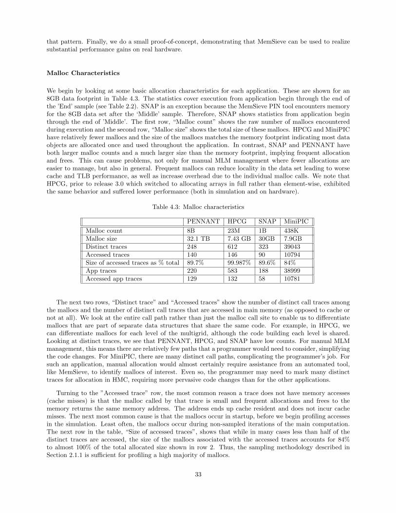
that pattern. Finally, we do a small proof-of-concept, demonstrating that MemSieve can be used to realizesubstantial performance gains on real hardware.

Malloc Characteristics

We begin by looking at some basic allocation characteristics for each application. These are shown for an8GB data footprint in Table 4.3. The statistics cover execution from application begin through the end ofthe ’End’ sample (see Table 2.2). SNAP is an exception because the MemSieve PIN tool encounters memoryfor the 8GB data set after the ‘Middle’ sample. Therefore, SNAP shows statistics from application beginthrough the end of ’Middle’. The first row, “Malloc count” shows the raw number of mallocs encounteredduring execution and the second row, “Malloc size” shows the total size of these mallocs. HPCG and MiniPIChave relatively fewer mallocs and the size of the mallocs matches the memory footprint indicating most dataobjects are allocated once and used throughout the application. In contrast, SNAP and PENNANT haveboth larger malloc counts and a much larger size than the memory footprint, implying frequent allocationand frees. This can cause problems, not only for manual MLM management where fewer allocations areeasier to manage, but also in general. Frequent mallocs can reduce locality in the data set leading to worsecache and TLB performance, as well as increase overhead due to the individual malloc calls. We note thatHPCG, prior to release 3.0 which switched to allocating arrays in full rather than element-wise, exhibitedthe same behavior and suffered lower performance (both in simulation and on hardware).

Table 4.3: Malloc characteristics

PENNANT HPCG SNAP MiniPIC

Malloc count 8B 23M 1B 438KMalloc size 32.1 TB 7.43 GB 30GB 7.9GBDistinct traces 248 612 323 39043Accessed traces 140 146 90 10794Size of accessed traces as % total 89.7% 99.987% 89.6% 84%App traces 220 583 188 38999Accessed app traces 129 132 58 10781

The next two rows, “Distinct trace” and “Accessed traces” show the number of distinct call traces amongthe mallocs and the number of distinct call traces that are accessed in main memory (as opposed to cache ornot at all). We look at the entire call path rather than just the malloc call site to enable us to differentiatemallocs that are part of separate data structures that share the same code. For example, in HPCG, wecan differentiate mallocs for each level of the multigrid, although the code building each level is shared.Looking at distinct traces, we see that PENNANT, HPCG, and SNAP have low counts. For manual MLMmanagement, this means there are relatively few paths that a programmer would need to consider, simplifyingthe code changes. For MiniPIC, there are many distinct call paths, complicating the programmer’s job. Forsuch an application, manual allocation would almost certainly require assistance from an automated tool,like MemSieve, to identify mallocs of interest. Even so, the programmer may need to mark many distincttraces for allocation in HMC, requiring more pervasive code changes than for the other applications.

Turning to the ”Accessed trace” row, the most common reason a trace does not have memory accesses(cache misses) is that the malloc called by that trace is small and frequent allocations and frees to thememory returns the same memory address. The address ends up cache resident and does not incur cachemisses. The next most common cause is that the mallocs occur in startup, before we begin profiling accessesin the simulation. Least often, the mallocs occur during non-sampled iterations of the main computation.The next row in the table, “Size of accessed traces”, shows that while in many cases less than half of thedistinct traces are accessed, the size of the mallocs associated with the accessed traces accounts for 84%to almost 100% of the total allocated size shown in row 2. Thus, the sampling methodology described inSection 2.1.1 is sufficient for profiling a high majority of mallocs.

33

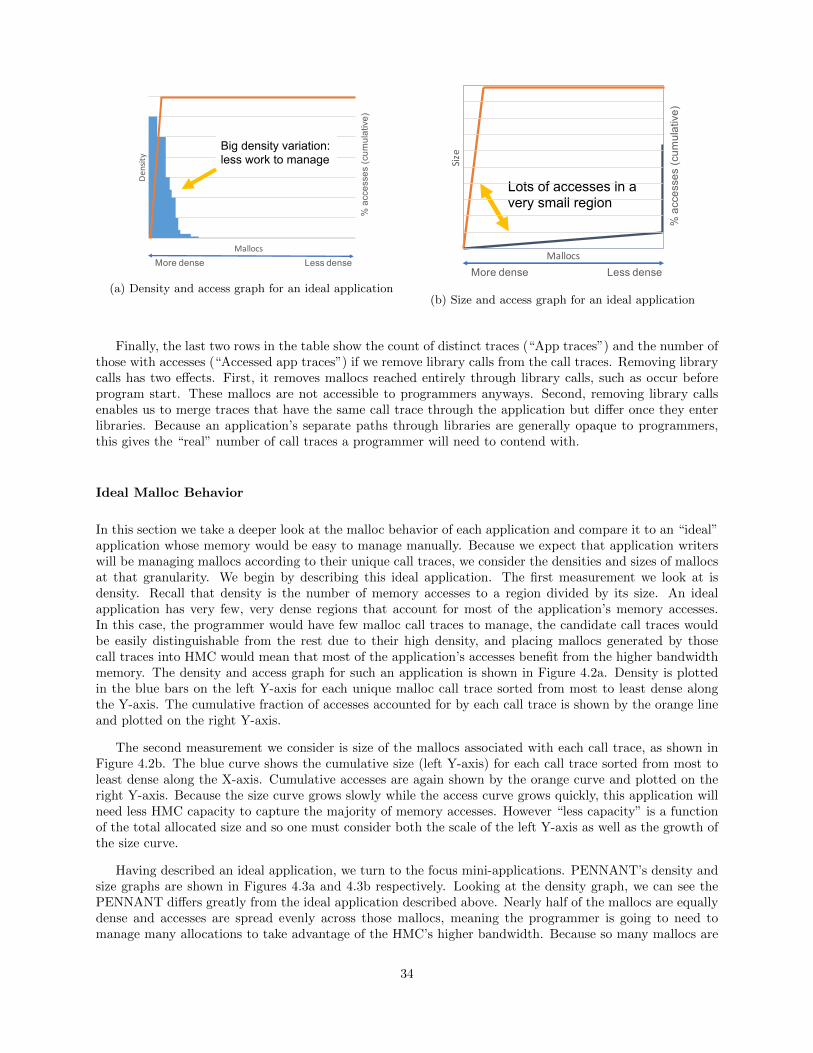
Density

Mallocs

Big density variation: less work to manage

% a

cces

ses

(cum

ulat

ive)

More dense Less dense

(a) Density and access graph for an ideal application

% a

cces

ses

(cum

ulat

ive)

Lots of accesses in a very small region

More dense Less dense

Size

Mallocs

(b) Size and access graph for an ideal application

Finally, the last two rows in the table show the count of distinct traces (“App traces”) and the number ofthose with accesses (“Accessed app traces”) if we remove library calls from the call traces. Removing librarycalls has two effects. First, it removes mallocs reached entirely through library calls, such as occur beforeprogram start. These mallocs are not accessible to programmers anyways. Second, removing library callsenables us to merge traces that have the same call trace through the application but differ once they enterlibraries. Because an application’s separate paths through libraries are generally opaque to programmers,this gives the “real” number of call traces a programmer will need to contend with.

Ideal Malloc Behavior

In this section we take a deeper look at the malloc behavior of each application and compare it to an “ideal”application whose memory would be easy to manage manually. Because we expect that application writerswill be managing mallocs according to their unique call traces, we consider the densities and sizes of mallocsat that granularity. We begin by describing this ideal application. The first measurement we look at isdensity. Recall that density is the number of memory accesses to a region divided by its size. An idealapplication has very few, very dense regions that account for most of the application’s memory accesses.In this case, the programmer would have few malloc call traces to manage, the candidate call traces wouldbe easily distinguishable from the rest due to their high density, and placing mallocs generated by thosecall traces into HMC would mean that most of the application’s accesses benefit from the higher bandwidthmemory. The density and access graph for such an application is shown in Figure 4.2a. Density is plottedin the blue bars on the left Y-axis for each unique malloc call trace sorted from most to least dense alongthe Y-axis. The cumulative fraction of accesses accounted for by each call trace is shown by the orange lineand plotted on the right Y-axis.

The second measurement we consider is size of the mallocs associated with each call trace, as shown inFigure 4.2b. The blue curve shows the cumulative size (left Y-axis) for each call trace sorted from most toleast dense along the X-axis. Cumulative accesses are again shown by the orange curve and plotted on theright Y-axis. Because the size curve grows slowly while the access curve grows quickly, this application willneed less HMC capacity to capture the majority of memory accesses. However “less capacity” is a functionof the total allocated size and so one must consider both the scale of the left Y-axis as well as the growth ofthe size curve.

Having described an ideal application, we turn to the focus mini-applications. PENNANT’s density andsize graphs are shown in Figures 4.3a and 4.3b respectively. Looking at the density graph, we can see thePENNANT differs greatly from the ideal application described above. Nearly half of the mallocs are equallydense and accesses are spread evenly across those mallocs, meaning the programmer is going to need tomanage many allocations to take advantage of the HMC’s higher bandwidth. Because so many mallocs are

34

0%

20%

40%

60%

80%

100%

00.51

1.52

2.53

3.54

%oftotalaccesses

Density

(accesses/by

te)

Malloc calltraces,frommosttoleastdense

DensityAccesses

(a) Density and access graph for PENNANT

0%

20%

40%

60%

80%

100%

0

8

16

24

32

%oftotalaccesses

Cumulativesiz

e(TB)

Malloc calltraces,frommosttoleastdense

Size(TB)Accesses

(b) Size and access graph for PENNANT

0%

20%

40%

60%

80%

100%

0

0.25

0.5

0.75

1

1.25

1.5

1.75

%ofto

talaccesses

Density

(accesses/by

te)

Malloccalltraces,frommosttoleastdense

Density

Accesses

(a) Density and access graph for HPCG

0%

20%

40%

60%

80%

100%

012345678

%oftotalaccesses

Cumulativesiz

e(GB)

Malloccalltraces,frommosttoleastdense

Size(MB)

Accesses

(b) Size and access graph for HPCG

dense, it is likely that dynamic migration between the HMC and DRAM will be be necessary. However,without looking at the behavior over time we cannot tell with certainty how the allocations are accessed indifferent application phases. MemSieve does have the ability to profile over time, but for this initial studywe did not pursue it. The second, size graph, is better at first glance as the many dense mallocs account fora small fraction of the overall size. Still, because the total size of mallocs is 30TB, a small fraction may notbe small enough to fit in HMC.

In contrast to PENNANT, HPCG demonstrates nearly ideal behavior. Its density graph, shown inFigure 4.4a has a steep cliff, far to the left indicating that the programmer will need to manage very fewallocations to capture both the majority of dense mallocs and the majority of accesses (shown by the redline). The size graph (Figure 4.4b) is less ideal. Although the most dense mallocs account for just 1/8thof the total memory, the programmer may not be able to fit all of the moderately dense mallocs in HMC.This means slightly lower performance especially at smaller HMC capacities, but compared to PENNANT,HPCG will require less work (and potentially no dynamic migration) to achieve the performance.

Figure 4.5a and Figure 4.5b show the density and size graphs, respectively, for SNAP. The density appearsideal however, the access curve resembles that of PENNANT – the densest mallocs account for a moderatefraction of overall accesses. Looking to the size graph we see that these densest mallocs are also quite small,about 1GB in total. As such it is likely that all of the dense mallocs will fit in even a small HMC. However,as the dense mallocs capture only about 50% of the accesses, steering the rest of the accesses to the HMCwill require considering sparser mallocs. Further, the size graph indicates that while most mallocs are small(i.e., flat curve), there are a few large, sparse mallocs and these correspond to large jumps in the accesscurve. Placing large, sparse mallocs in a limited size HMC will be difficult and therefore for SNAP, onemay need to consider a smaller granularity than mallocs to capture more accesses. Overall SNAP presents amixed picture. One should be able to easily fit the densest mallocs into HMC, but doing so will only capturehalf of the accesses. Capturing the remaining accesses will require more work.

Finally, we analyze MiniPIC’s allocation behavior. Figure 4.6a shows MiniPIC’s density graph. Ofthe applications analyzed, MiniPIC is the least ideal. The majority of dense mallocs account for very fewaccesses and so placing the dense mallocs in HMC is likely to have no effect on performance. The size graph(Figure 4.6b is similarly non-ideal. The size and access curves are both far to the right, indicating that notonly must one consider the sparse mallocs to capture the majority of memory accesses, the sparse mallocs

35

0%

20%

40%

60%

80%

100%

0

0.5

1

1.5

2

2.5

Precen

toftotalac

cesses

(cum

ulative)

Density

(accesses/by

te)

Malloccallsites,frommosttoleastdense

Density

Accesses

(a) Density and access graph for SNAP

0%

20%

40%

60%

80%

100%

0

5

10

15

20

25

30

Percen

toftotalaccesses

(cum

ulative)

Cumulativesiz

e(GB)

Malloccallsites,frommosttoleastdense

Size(GB)Accesses

(b) Size and access graph for SNAP

0%

20%

40%

60%

80%

100%

0

0.1

0.2

0.3

0.4

0.5

0.6

Precen

toftotalac

cesses

(cum

ulative)

Density

(accesses/by

te)

Malloccallsites,frommosttoleastdense

Density

Accesses

(a) Density and access graph for MiniPIC

0%

20%

40%

60%

80%

100%

0

1

2

3

4

5

6

7

Percen

toftotalaccesses

(cum

ulative)

Cumulativesiz

e(GB)

Malloccallsites,frommosttoleastdense

Size(GB)Accesses

(b) Size and access graph for MiniPIC

are large and therefore likely difficult to place in HMC. While MiniPIC showed no performance improvementin Section 3.1 and therefore we do not consider it further, these graphs indicate that even if it did benefitfrom HMC, it would not be easy to capture the performance with a small HMC-to-DRAM ratio.

Architecture Effect on Dense Mallocs

Our last analysis looks at the effect of the cache architecture and application input on which mallocs areconsidered dense. For manual allocation this is important, as the programmer would need to redo theallocation management if it varied with either architecture or input. Input is arguably a bigger problem,as applications are likely to be run on few architectures, but the inputs may vary widely. Still, variancedue to either architecture or input increases the work of the programmer and makes manual allocation lessappealing.

Figures 4.7 and 4.8 show the variance in the top malloc trace ranking for PENNANT and HPCG betweentwo data set sizes. Similarity on the Y-axis is measured as the fraction of the top N malloc traces (for Nshown along the X-axis) that are the same for both the smaller and larger data footprint. For example, a50% similarity at N=2 would mean that one of the top two traces match in the rankings for the smallerand larger data footprint. While both graphs show some differences in the top 20-30, overall the sets ofdense traces are similar. For perspective, in the next section where we manually place mallocs, we generallyconsider the top 40-50 traces. Thus, while for very small HMCs the variation may have effect, for largerHMCs like those studied here, the differences in ranking do not greatly affect malloc placement. This isadvantageous as it means a programmer can profile and the application once and apply the results to a widerange of inputs. For HPCG at N larger than 60, the similarity does start to drop off. This occurs becausethe malloc traces ranked ¿60 tend to have few accesses (e.g., less than ten) and small simulation variationscan be the difference between the trace being cached or not.

We now look at the variance due to architecture. For this experiment we ran HPCG and PENNANTusing MemSieve representations of both the lightweight and heavyweight cache hierarchy. Figure 4.9 showsthe resulting variance for PENNANT and Figure 4.10 shows HPCG’s variance. As in the previous set ofgraphs, the X-axis shows the number of malloc traces compared and the Y-axis shows the percent of malloctraces in each of the lightweight and heavyweight ranking that match. For PENNANT and HPCG there

36

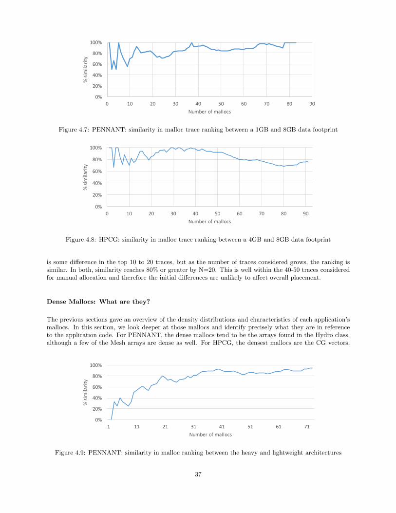
0%

20%

40%

60%

80%

100%

0 10 20 30 40 50 60 70 80 90

%similarity

Numberofmallocs

Figure 4.7: PENNANT: similarity in malloc trace ranking between a 1GB and 8GB data footprint

0%

20%

40%

60%

80%

100%

0 10 20 30 40 50 60 70 80 90

%similarity

Numberofmallocs

Figure 4.8: HPCG: similarity in malloc trace ranking between a 4GB and 8GB data footprint

is some difference in the top 10 to 20 traces, but as the number of traces considered grows, the ranking issimilar. In both, similarity reaches 80% or greater by N=20. This is well within the 40-50 traces consideredfor manual allocation and therefore the initial differences are unlikely to affect overall placement.

Dense Mallocs: What are they?

The previous sections gave an overview of the density distributions and characteristics of each application’smallocs. In this section, we look deeper at those mallocs and identify precisely what they are in referenceto the application code. For PENNANT, the dense mallocs tend to be the arrays found in the Hydro class,although a few of the Mesh arrays are dense as well. For HPCG, the densest mallocs are the CG vectors,

0%

20%

40%

60%

80%

100%

1 11 21 31 41 51 61 71

%similarity

Numberofmallocs

Figure 4.9: PENNANT: similarity in malloc ranking between the heavy and lightweight architectures

37

Figure 4.10: HPCG: similarity in malloc ranking between the heavy and lightweight architectures

followed by some of the structures associated with levels of the multigrid. In general, finer levels of the gridhave denser mallocs than coarser ones. But, this is not a strict rule. For example the textitAxf vector is onedensest mallocs regardless of grid level.

In SNAP, many of the densest allocations are working arrays allocated in the Solvar module. Other denseallocations include the leakage arrays and flux moment arrays. Finally, in MiniPIC the ParticleTypeList isthe densest allocation, followed by some of the face and edge maps. These include the boundary face map,owned boundary edge map, and owned face map.

Translating MemSieve to Hardware

We envision that the MemSieve tool will be useful for programmers trying to determine which allocationsare the best candidates for HMC (or HBM) allocation. In this section we take a look at that workflow andvalidate that MemSieve’s suggestions do result in performance improvements on real hardware. For thisstudy we looked at MiniFE rather than one of the four focus mini-apps. The major reason for this is thatMiniFE is simpler than the focus mini-apps so that manually editing it for allocation on real hardware iseasier. Running MiniFE through MemSieve revealed that four of the top five ranked mallocs were Vectors.The sixth-ranked malloc was the array, which is likely too big to place in the Knight’s Landing’s HBM.The remaining top ten mallocs were comprised of calls related to OpenMP for loops which are difficultto manually allocate since the allocation is done by the OpenMP library. To test MemSieve’s suggestionstherefore, we manually edited MinIFE to place the Vectors in HBM. Figure 4.11 shows the results. On theleft is the performance of MiniFE on the Knight’s Landing when running completely out of the DRAM.Performance is normalized to this configuration. In the middle is the performance of MiniFE when runningcompletely out of the HBM. While this is the ideal case, the HBM is too small for realistic problem sizesto fall in this category. Therefore, a hybrid approach is needed, as shown on the right. This bar showsthe performance of MiniFE when the Vectors, per MemSieve’s recommendation, are manually allocated toHBM. In this case, we see a significant, 1.5X speedup over DRAM only.

Processing-In-Memory and MemSieve

We finish our discussion of MemSieve by touching briefly on the subject of processing-in-memory (PIM).Because HMCs have a logic layer under the DRAM stack, they are ideal candidate technologies for imple-menting PIM. However, the question is not the capability of HMCs to support PIM, but rather what kindof PIM applications might benefit from. One way to approach this question is to look at which applicationallocations are likely to be HMC-resident. Allocations that are largely cache-resident or move between cachesand memory would increase PIM overhead by requiring extra flushes and coherence actions to ensure coher-ent PIM. On the other hand, allocations that are likely to be resident in DRAM are not candidates for PIMas operating on them would require migrating the data to HMC. Fortunately, MemSieve can answer this

38

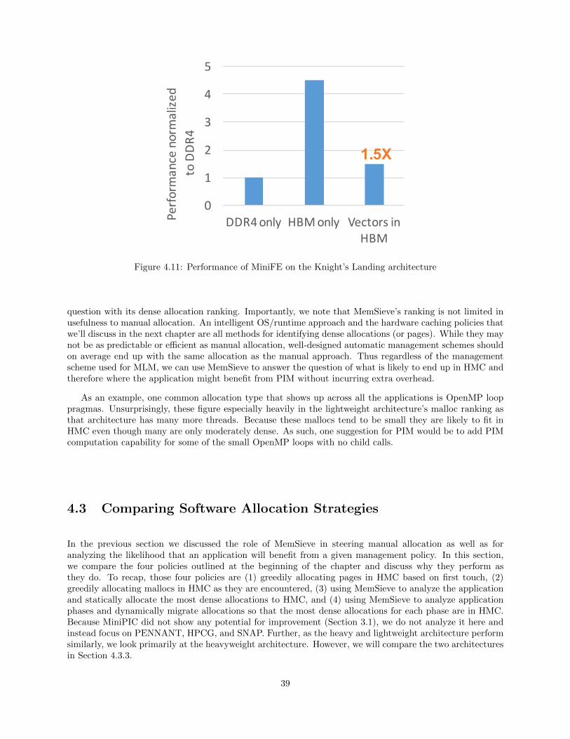
0

1

2

3

4

5

DDR4only HBMonly VectorsinHBM

Perfo

rmancenormalize

dtoDDR

4

1.5X

Figure 4.11: Performance of MiniFE on the Knight’s Landing architecture

question with its dense allocation ranking. Importantly, we note that MemSieve’s ranking is not limited inusefulness to manual allocation. An intelligent OS/runtime approach and the hardware caching policies thatwe’ll discuss in the next chapter are all methods for identifying dense allocations (or pages). While they maynot be as predictable or efficient as manual allocation, well-designed automatic management schemes shouldon average end up with the same allocation as the manual approach. Thus regardless of the managementscheme used for MLM, we can use MemSieve to answer the question of what is likely to end up in HMC andtherefore where the application might benefit from PIM without incurring extra overhead.

As an example, one common allocation type that shows up across all the applications is OpenMP looppragmas. Unsurprisingly, these figure especially heavily in the lightweight architecture’s malloc ranking asthat architecture has many more threads. Because these mallocs tend to be small they are likely to fit inHMC even though many are only moderately dense. As such, one suggestion for PIM would be to add PIMcomputation capability for some of the small OpenMP loops with no child calls.

4.3 Comparing Software Allocation Strategies

In the previous section we discussed the role of MemSieve in steering manual allocation as well as foranalyzing the likelihood that an application will benefit from a given management policy. In this section,we compare the four policies outlined at the beginning of the chapter and discuss why they perform asthey do. To recap, those four policies are (1) greedily allocating pages in HMC based on first touch, (2)greedily allocating mallocs in HMC as they are encountered, (3) using MemSieve to analyze the applicationand statically allocate the most dense allocations to HMC, and (4) using MemSieve to analyze applicationphases and dynamically migrate allocations so that the most dense allocations for each phase are in HMC.Because MiniPIC did not show any potential for improvement (Section 3.1), we do not analyze it here andinstead focus on PENNANT, HPCG, and SNAP. Further, as the heavy and lightweight architecture performsimilarly, we look primarily at the heavyweight architecture. However, we will compare the two architecturesin Section 4.3.3.

39

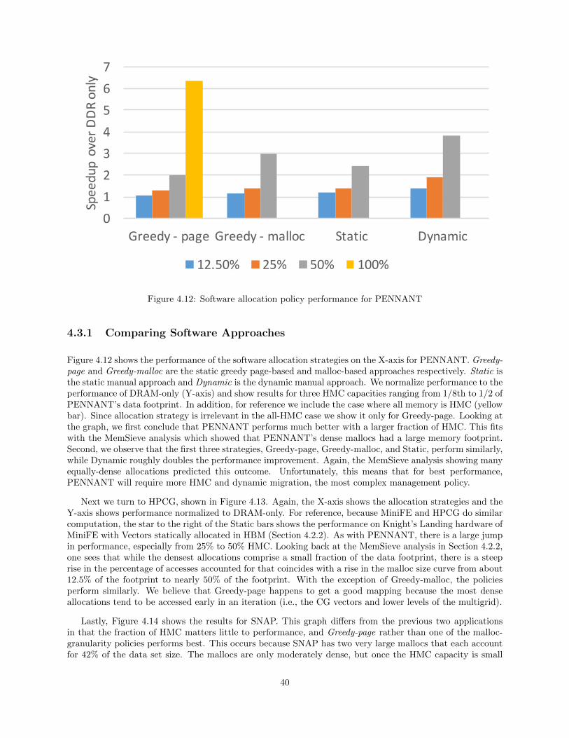
01234567

Greedy- page Greedy- malloc Static Dynamic

SpeedupoverDDR

only

12.50% 25% 50% 100%

Figure 4.12: Software allocation policy performance for PENNANT

4.3.1 Comparing Software Approaches

Figure 4.12 shows the performance of the software allocation strategies on the X-axis for PENNANT. Greedy-page and Greedy-malloc are the static greedy page-based and malloc-based approaches respectively. Static isthe static manual approach and Dynamic is the dynamic manual approach. We normalize performance to theperformance of DRAM-only (Y-axis) and show results for three HMC capacities ranging from 1/8th to 1/2 ofPENNANT’s data footprint. In addition, for reference we include the case where all memory is HMC (yellowbar). Since allocation strategy is irrelevant in the all-HMC case we show it only for Greedy-page. Looking atthe graph, we first conclude that PENNANT performs much better with a larger fraction of HMC. This fitswith the MemSieve analysis which showed that PENNANT’s dense mallocs had a large memory footprint.Second, we observe that the first three strategies, Greedy-page, Greedy-malloc, and Static, perform similarly,while Dynamic roughly doubles the performance improvement. Again, the MemSieve analysis showing manyequally-dense allocations predicted this outcome. Unfortunately, this means that for best performance,PENNANT will require more HMC and dynamic migration, the most complex management policy.

Next we turn to HPCG, shown in Figure 4.13. Again, the X-axis shows the allocation strategies and theY-axis shows performance normalized to DRAM-only. For reference, because MiniFE and HPCG do similarcomputation, the star to the right of the Static bars shows the performance on Knight’s Landing hardware ofMiniFE with Vectors statically allocated in HBM (Section 4.2.2). As with PENNANT, there is a large jumpin performance, especially from 25% to 50% HMC. Looking back at the MemSieve analysis in Section 4.2.2,one sees that while the densest allocations comprise a small fraction of the data footprint, there is a steeprise in the percentage of accesses accounted for that coincides with a rise in the malloc size curve from about12.5% of the footprint to nearly 50% of the footprint. With the exception of Greedy-malloc, the policiesperform similarly. We believe that Greedy-page happens to get a good mapping because the most denseallocations tend to be accessed early in an iteration (i.e., the CG vectors and lower levels of the multigrid).

Lastly, Figure 4.14 shows the results for SNAP. This graph differs from the previous two applicationsin that the fraction of HMC matters little to performance, and Greedy-page rather than one of the malloc-granularity policies performs best. This occurs because SNAP has two very large mallocs that each accountfor 42% of the data set size. The mallocs are only moderately dense, but once the HMC capacity is small

40

0

1

2

3

4

5

6

Greedy- page Greedy- malloc Static Dynamic

SpeedupoverDDR

only

12.50% 25% 50% 100%

MiniFE w/ Vectors

Figure 4.13: Software allocation policy performance for HPCG

enough that neither fits, the malloc policies capture the same mallocs. The page-based policy on the otherhand is able to capture part of these mallocs, resulting in better HMC utilization and higher performance.This points to a need for a code change if the malloc-policies are to perform well. Large mallocs lead toinefficient use of the HMC. It is also possible that large mallocs hide smaller dense and less dense regionswithin them.

Overall, the greedy policies perform well, but this statement comes with an important caveat. Thestudied mini-apps, while more complex than many, are not real applications. Full applications with manyexecution phases and allocations that occur throughout execution are unlikely to perform well with greedybecause only the early allocations and phases will benefit from the HMC. PENNANT hints at this case, whereallocations occur and the set of dense data structures changes throughout execution. As such, support fordynamic migration is essential, whether application- or OS-managed.

4.3.2 Effectiveness of Manual Allocation

We now look slightly deeper at the effect of manual allocation on the spread of accesses to the differentmemory levels. Table 4.4 shows the fraction of memory accesses that went to HMC instead of DRAM foreach of the benchmarks, policies, and HMC capacities in the preceding section

Table 4.4: Fraction of accesses to HMC compared to DDR

Policy Greedy-page Greedy-malloc Static DynamicCapacity 12.5% 25% 50% 12.5% 25% 50% 12.5% 25% 50% 12.5% 25% 50%

SNAP 34% 47% 68% 38% 52% 52% 36% 52% 49% 40% 44% 44%HPCG 26% 49% 92% 5% 29% 75% 23% 47% 93% 23% 49% 93%PENNANT 20% 34% 62% 15% 30% 55% 20% 33% 67% 38% 47% 87%

41

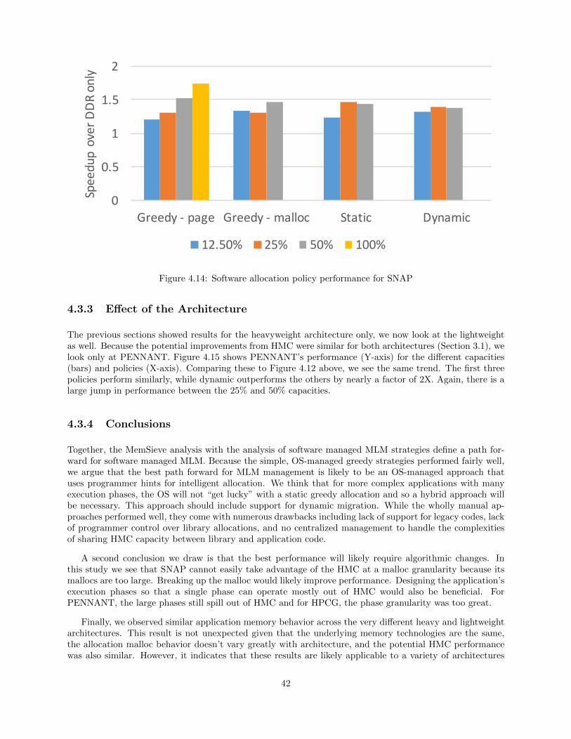
0

0.5

1

1.5

2

Greedy- page Greedy- malloc Static Dynamic

SpeedupoverDDR

only

12.50% 25% 50% 100%

Figure 4.14: Software allocation policy performance for SNAP

4.3.3 Effect of the Architecture

The previous sections showed results for the heavyweight architecture only, we now look at the lightweightas well. Because the potential improvements from HMC were similar for both architectures (Section 3.1), welook only at PENNANT. Figure 4.15 shows PENNANT’s performance (Y-axis) for the different capacities(bars) and policies (X-axis). Comparing these to Figure 4.12 above, we see the same trend. The first threepolicies perform similarly, while dynamic outperforms the others by nearly a factor of 2X. Again, there is alarge jump in performance between the 25% and 50% capacities.

4.3.4 Conclusions

Together, the MemSieve analysis with the analysis of software managed MLM strategies define a path for-ward for software managed MLM. Because the simple, OS-managed greedy strategies performed fairly well,we argue that the best path forward for MLM management is likely to be an OS-managed approach thatuses programmer hints for intelligent allocation. We think that for more complex applications with manyexecution phases, the OS will not “get lucky” with a static greedy allocation and so a hybrid approach willbe necessary. This approach should include support for dynamic migration. While the wholly manual ap-proaches performed well, they come with numerous drawbacks including lack of support for legacy codes, lackof programmer control over library allocations, and no centralized management to handle the complexitiesof sharing HMC capacity between library and application code.

A second conclusion we draw is that the best performance will likely require algorithmic changes. Inthis study we see that SNAP cannot easily take advantage of the HMC at a malloc granularity because itsmallocs are too large. Breaking up the malloc would likely improve performance. Designing the application’sexecution phases so that a single phase can operate mostly out of HMC would also be beneficial. ForPENNANT, the large phases still spill out of HMC and for HPCG, the phase granularity was too great.

Finally, we observed similar application memory behavior across the very different heavy and lightweightarchitectures. This result is not unexpected given that the underlying memory technologies are the same,the allocation malloc behavior doesn’t vary greatly with architecture, and the potential HMC performancewas also similar. However, it indicates that these results are likely applicable to a variety of architectures

42

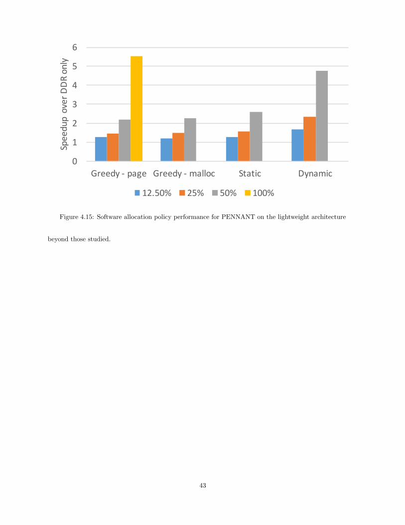
0

1

2

3

4

5

6

Greedy- page Greedy- malloc Static Dynamic

SpeedupoverDDR

only

12.50% 25% 50% 100%

Figure 4.15: Software allocation policy performance for PENNANT on the lightweight architecture

beyond those studied.

43

44

Chapter 5

Automatic Management

Manual management is advantageous because it requires no modification to the hardware, however it doesrequire programmer effort and / or knowledge. Thus, it is worth exploring MLM which is managed withoutany programmer effort. In automatic management, the hardware, operating system, runtime, or somecombination thereof move data between the levels of memory without user guidance.

In this chapter, we explore several automatic MLM management policies.

5.1 Background

5.1.1 Related Work

There is a wealth of related work on automatic paging algorithms and cache policies. For caches, most worksemphasize different replacement policies, such as Least Recently Used (LRU), or pseudo-LRU for SRAMcaches[7]. A variety of virtual memory paging schemes have been explored such as simple FIFOs, LRU,multiple queue systems[9], or adaptive models[3].

Multi-level Memory has explored the combination of DRAM and NVRAM[17] with demand paging,sometimes using dynamic policies[12]. [16] explores hybrid policies to reduce energy. In particular, itexplores using historical page access information (HRank) to performs bulk swaps at regular intervals andan inclusive demand paging policy (PCache). Other work[1] examines user-directed management of MLM.

5.1.2 Key Differences

This work differs primarily in that it focuses on the addition policy rather than the replacement policy. Inmost systems (e.g. SRAM caches backed by DRAM or DRAM backed by hard disk) the relative latency ofthe faster storage is so much lower than the backing store that the best addition policy is almost always asimple “always add” policy. In an MLM system comprised of DDR + fast stacked memory that is not thecase.

The MLM management problem is a subset of the general caching / paging problem. This problemconsists of two parts: addition policies, that determine when a block of data is moved to the faster memory,and replacement policies, that determine when a block of data in the faster memory should be moved tothe slower memory. The MLM problem is similar to the management of processor SRAM caches or virtualmemory (VM). However, due to the massive differences in latency between levels, both SRAM caches andVM must bring data into the closer memory before it is used. In these systems, the addition policy couldbe described as “Always Add.”

In MLM, the latency of the Fast memory may not be dramatically different from traditional DDR DRAM.Thus, there are many cases where it may make sense to leave a data block in the slower memory if it is

45

not going to be used frequently. This saves the overhead of transferring between levels of memory. Earlysimulations of several benchmarks of a system with 128 pages of fast memory using a simple always addpolicy found that performance was reduced by 9% to 61% (average: 52%) poor policies can turn MLM froma benefit into a liability.

5.2 Early Analysis

To develop potential policies, we began by analyzing several applications’ (Section 2.1) memory accesspatterns.

5.2.1 Access Patterns Within A Page

Using the infrastructure created for [8], we examined how post-cache memory accesses are distributed withina page. The analysis filter records each access to a page and compares it with the last access to that page. Itthen computes the offset (∆ = Addrnew − Addrold) and classifies the new access into one of five categories:Same Address (∆ = 0), next cache line, ∆ = 1, ‘jump forward” (∆ > 1), previous cache line (∆ = −1), or“jump back” (∆ < −1).

Each page was placed in a five dimensional space based on the percentage of memory accesses that fallinto each category. A k-means clustering algorithm was applied to the classified pages for each applicationto identify “typical” pages. Figure 5.1 shows the center points of four clusters for the access patterns forthree applications. For each center, the graph shows the five “directions” that the next memory access takes(∆ = 0,1,−1,> 1,< −1) and the percent of memory accesses that fall into that cluster.

For example, in Lulesh 64.1% of accesses go to pages which are dominated by an access pattern that isoverwhelmingly incrementing through memory, but there are a seizable number of accesses (26.9%) which goto pages that tend towards increment, but have a third of their accesses either jumping ahead or behind bysome amount. In contrast, MiniFE is almost completely dominated by pages that are simply incrementingthrough memory.

This indicates that many applications have a significant “streaming” component – large number of pageswhich are accessed sequentially. Because so many pages have a strong ∆ = 1 component, it should bepossible to detect “streaming” pages by noting a relatively short series of consecutive positive incrementalaccesses.

5.2.2 Multithreaded Access

We also wished to examine how many threads of execution access a given page. The goal of this analysiswas to determine suitable page sizes. Ideally, a page size should be large enough that per-page meta-data islimited, but small enough that patterns (e.g. scans) are preserved and swap time is limited. We theorize thatminimizing the number of threads that are accessing a page would be beneficial. If fewer threads are accessinga page, post-cache hardware is more likely to identify simple patterns (e.g. linear scans). Additionally, apage with fewer threads accessing it can probably be swapped from one level of memory to another withoutdisrupting as many threads.

Using SST, we performed an analysis for several mini-apps. For each page in memory we looked at howmany unique threads accessed that page, and how many times each thread accessed that page. For thisanalysis we only examined post-cache accesses (i.e. main memory accesses).

Across CoMD (Figure 5.2(a)), Lulesh (Figure 5.2(b)), and MiniFE (Figure 5.2(c)) 4KB pages are accessedby only a small number of threads – generally one or two threads. Even in the case of Lulesh, which has a

46

Figure 5.1: Intra-page access patterns

(a)

Figure 1: Intra-Page Access Patterns

(a)

(b)

(c)

Figure 2: Thread Use Per Page for (a) CoMD (b) Lulesh and (c) MiniFE

(b)

Figure 1: Intra-Page Access Patterns

(a)

(b)

(c)

Figure 2: Thread Use Per Page for (a) CoMD (b) Lulesh and (c) MiniFE

(c)

Figure 1: Intra-Page Access Patterns

(a)

(b)

(c)

Figure 2: Thread Use Per Page for (a) CoMD (b) Lulesh and (c) MiniFE

Figure 5.2: Thread use per page for (a) CoMD (b) Lulesh and (c) MiniFE

sizable number of pages accessed by multiple threads, the vast bulk of accesses go to pages that are touchedby only one or two threads.

47

Core

L1

Core

L1

L2

Core

L1

Core

L1

Merlin Router

Directory Controller

Core

L1

Core

L1

L2

Core

L1

Core

L1

DDR

Ariel Trace Capture

PIN

"Fast" Memory

MLM Unit

Mapping Table

DMAPolicy

Dispatcher

Figure 5.3: Proposed architecture and simulation model

5.3 Policies

To explore multiple MLM policies, we propose a simple, self-contained architectural block, the MLM Unit,which dispatches main memory accesses to either traditional DDR DRAM or a “Fast” memory. Figure 5.3shows the proposed block, which is comprised of three subunits:

• Policy Dispatcher: The control unit of the block, which decides if a given memory page should belocated in the DDR or fast memory, swaps pages as needed, and dispatches incoming memory accessesappropriately. The addition and replacement policies are detailed below (Sections 5.3.1 and 5.3.2).

• Mapping Table: A TLB-like structure (in the sense that it contains metadata about each memorypage) which records which pages reside in fast memory, as well as policy-specific meta-data for eachpage.

• DMA: A unit to transfer pages between the DDR and fast memory without involving the CPU orcoherent cache hierarchy.

The MLM Unit attaches to the memory hierarchy after the directory controller, so all coherency decisionshave already been made. Because there is only one valid copy in the backing store (either in the DRAMmemory or “Fast” memory), the MLM Unit does not require additional coherency tracking, nor does thecache coherency protocol need to be modified to support MLM. Additionally, the mapping table data is onlyused locally and does not require complex management like a TLB.

Though the DMA subunit and certain updates to page metadata require hardware support, the actualpolicy decisions could be made purely in hardware or with more explicit software, operating system, orruntime control.

5.3.1 Addition Policies

Addition policies determine if a candidate page which is being accessed should be added to the “fast” memory.Seven addition policies were implemented. Many of these policies require a count of accesses be kept foreach page in memory. This count, touchCount, is reset every 5ms. The policies we examined are:

48

• addT (Threshold) is a simple threshold policy. If the candidate page’s touchCount is greater than agiven threshold it will be added to the “fast” memory.

• addMFU (Most Frequently Used) If a candidate page’s touchCount is greater than the lowest touchCountof all pages currently in fast memory, the candidate page will be added. The overhead of this policywould probably be prohibitive in practice, but it is included for completeness. This policy is similar toHRank [16], but is performed continuously and for individual pages instead of multi-page transfers attimed intervals.

• addRAND (Random) Each time it is touched, the candidate page has a 1-in-8192 chance of beingadded. This probability was chosen after a search of parameters to give good performance for the givenapplications.

• addMRPU (More Recent Previous Use) If the candidate page’s last touch was more recent than theleast previously used page in fast memory it is added. This requires that each page in memory bemarked with the time of its last access.

• addMFPRU (More Frequent, More Recent Previous Use) As addMRPU, but only add the candidatepage if it also has a higher touchCount than the least recently used page in fast memory.

• addSC (Stream Conscious) A policy inspired by the access patterns detected in Section 5.2.1, addSCis similar to addT, but also detects streaming pages. If the last six accesses to a page have been tosequential cache line addresses (i.e. ∆ = 1), then it only has a 1-in-1024 chance of being added. Thiswould require additional metadata (sequential access count, last cache line address) to be stored foreach page.

• addSCF (Stream Conscious-Frequency) Operates as addSC, but only add the candidate page if it alsohas a higher touchCount than the least recently used page in fast memory.

In addition, all policies include “swap throttling” in which they will not start swapping a page to fastmemory if the DRAM transaction queue is full.

5.3.2 Replacement Policies

Replacement policies determine which page should be removed from “fast” memory to make room for a newpage. We looked at six policies:

• FIFO (First In / First Out) When a new page is added to fast memory it is added to the front of alist. When a page needs to be removed from fast memory, the page is chosen from the back of the list.

• LRU (Least Recently Used) New pages are added to the front of a list, and pages are removed fromthe back of the list. Whenever a page is accessed it is moved to the front of the list.

• LFU (Least Frequently Used) The accompanying replacement policy for addMFU. Replace the leastfrequently used page.

• LFU8 (Least Frequently Used, 8bit) Like LFU, but the touchCount is an 8-bit saturating counter.

• BiLRU (Bi-Modal Least Recently Used) Like LRU, but 1 out of 128 pages are placed at the back ofthe replacement list.

• SCLRU: (Stream Conscious Least Recently Used) Like LRU, but streaming pages are put at the backof the list when they are added and they are not moved to the front of the list when they are touched.

5.4 Early Results

To quickly test different policies, our first simulations swept each application using combinations of the sevenaddition policies and six replacement policies. For Lulesh and MiniFE (Figure 5.4) the addMFPRU, ad-dMFU, and addSCF addition policies perform best, with addRAND performing reasonably well for MiniFE.

49

The BiLRU, LRU, and SCLRU replacement policies have very similar performance. FIFO is slightly worse– about 5-6% slower.

For the two molecular dynamics applications, CoMD and Lammps, the results (Figure 5.5) are similar.The addMFPRU, addMFU, and addSCF addition policies perform best, with addRAND slightly (2-4%)slower. For these applications the choice of replacement policy is even less critical, with less than 1%performance difference between the different policies.

These results show several trends. “Frequency” based addition policies (addMFRPU, addMFU, andaddSCF) perform best, though a properly tuned random policy can be reasonably effective. Most striking,as long as the addition policy is reasonable, the replacement policy has a rather limited effect on performance.Even a simple FIFO policy is usually within a few percent of the best policy.

The relative unimportance of the replacement policy is also shown by the next set of experiments inwhich the threshold for the addT policy was varied for each application (Figure 5.6). Applications tendedto perform better with higher thresholds. However, they did evidence diminishing returns and the bestthreshold appears to differ for each application.

Lastly, we explored the effectiveness of “swap throttling” – not issuing swaps to or from fast memorywhen the DRAM was busy. While throttling did not have a major impact on most policies, it did havea significant impact on the simple addT (threshold) policy (Figure 5.7). Turning off throttling decreasedLammps performance by 32% and Lulesh by 18%.

5.4.1 Analysis

The primary finding of these experiments is that the addition policy is more important than the replacementpolicy. Different addition policies, or even different addition policy parameters, can have a dramatic impacton performance, while the replacement policy has a more muted effect. Most likely, this is because bringingpages in which are not frequently used entails a high transfer cost and, unlike a conventional SRAM cache,is not as necessary.

Of the analyzed policies, there are clear “winners.” The addMFRPU, addMFU, addRAND, and addSCFall provide good performance over the range of test applications. Each of them present different trade-offs inthe amount of meta-data which must be gathered and stored. The addSCF and addMFRPU policies providebetter performance, but require collection of touchCounts for each page. While addRAND’s performance isabout 5% lower on average, it does not require metadata collection or streaming analysis.

For these small applications, the “stream aware” policies show promise. Applications which have a numberof pages which show streaming behavior (e.g. MiniFE in Figure 5.1) gain a small amount of performancewith stream aware policies.

Optimizing policies requires several trade-offs. Simply maximizing he “hit rate” on the fast memoryis not sufficient to ensure higher performance. For example the addSC/SCLRU policies actually give ahigher hit rate (≈40%) than addSCF/SCLRU (≈12%), even though addSCF/SCLRU provides better overallapplication performance. However, addSC’s lower criteria for addition means that addSC/SCLRU generates20-70 times more page swaps. These consume considerable bandwidth and hurt performance, even withswap throttling.

5.5 Large Application Results

Guided by the results from smaller applications, we performed simulations on larger applications (Section 2.1)focusing on a constrained set of policies.

50

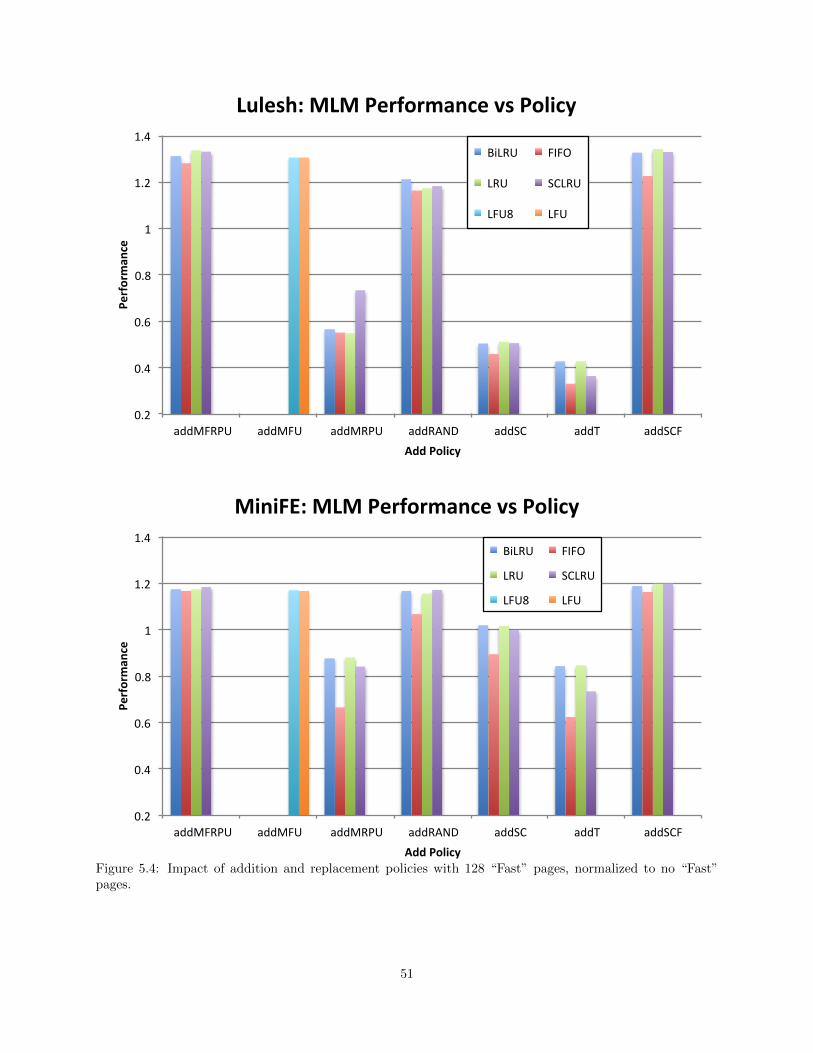
0.2

0.4

0.6

0.8

1

1.2

1.4

addMFRPU addMFU addMRPU addRAND addSC addT addSCF

Performan

ce

AddPolicy

Lulesh:MLMPerformancevsPolicy

BiLRU FIFO

LRU SCLRU

LFU8 LFU

0.2

0.4

0.6

0.8

1

1.2

1.4

addMFRPU addMFU addMRPU addRAND addSC addT addSCF

Performan

ce

AddPolicy

MiniFE:MLMPerformancevsPolicy

BiLRU FIFO

LRU SCLRU

LFU8 LFU

Figure 5.4: Impact of addition and replacement policies with 128 “Fast” pages, normalized to no “Fast”pages.

51

0.2

0.4

0.6

0.8

1

1.2

addMFRPU addMFU addMRPU addRAND addSC addT addSCF

Performan

ce

AddPolicy

CoMD:MLMPerformancevsPolicy

BiLRU FIFO

LRU SCLRU

LFU8 LFU

0.2

0.4

0.6

0.8

1

1.2

addMFRPU addMFU addMRPU addRAND addSC addT addSCF

Performan

ce

AddPolicy

Lammps:MLMPerformancevsPolicy

BiLRU FIFO

LRU SCLRU

LFU8 LFU

Figure 5.5: Impact of addition and replacement policies with 128 “Fast” pages, normalized to no “Fast”pages.

52

0.5

1.5

2.5

3.5

0 200 400 600 800 1000

Performan

ce

Threshold

MLMPerformacevs.Threshold(addT/LRU)

CoMDlammpsluleshminiFE

Figure 5.6: Impact of threshold value, normalized to T=0, LRU replacement

0

0.2

0.4

0.6

0.8

1

CoMD lammps lulesh miniFE

Performan

ce

SwapThro0ling

Thro;le

NoThro;le

Figure 5.7: Impact of swap throttling (LRU replacement)

53

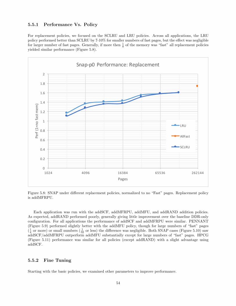
5.5.1 Performance Vs. Policy

For replacement policies, we focused on the SCLRU and LRU policies. Across all applications, the LRUpolicy performed better than SCLRU by 7-10% for smaller numbers of fast pages, but the effect was negligiblefor larger number of fast pages. Generally, if more then 1

8 of the memory was “fast” all replacement policiesyielded similar performance (Figure 5.8).

0

0.2

0.4

0.6

0.8

1

1.2

1.4

1.6

1.8

2

1024 4096 16384 65536 262144

Perf(1=nofastmem

)

Pages

Snap-p0 Performance:Replacement

LRU

AllFast

SCLRU

Figure 5.8: SNAP under different replacement policies, normalized to no “Fast” pages. Replacement policyis addMFRPU.

Each application was run with the addSCF, addMFRPU, addMFU, and addRAND addition policies.As expected, addRAND performed poorly, generally giving little improvement over the baseline DDR-onlyconfiguration. For all applications the performance of addSCF and addMFRPU were similar. PENNANT(Figure 5.9) performed slightly better with the addMFU policy, though for large numbers of “fast” pages( 14 or more) or small numbers ( 1

32 or less) the difference was negligible. Both SNAP cases (Figure 5.10) sawaddSCF/addMFRPU outperform addMFU substantially except for large numbers of “fast” pages. HPCG(Figure 5.11) performance was similar for all policies (except addRAND) with a slight advantage usingaddSCF.

5.5.2 Fine Tuning

Starting with the basic policies, we examined other parameters to improve performance.

54

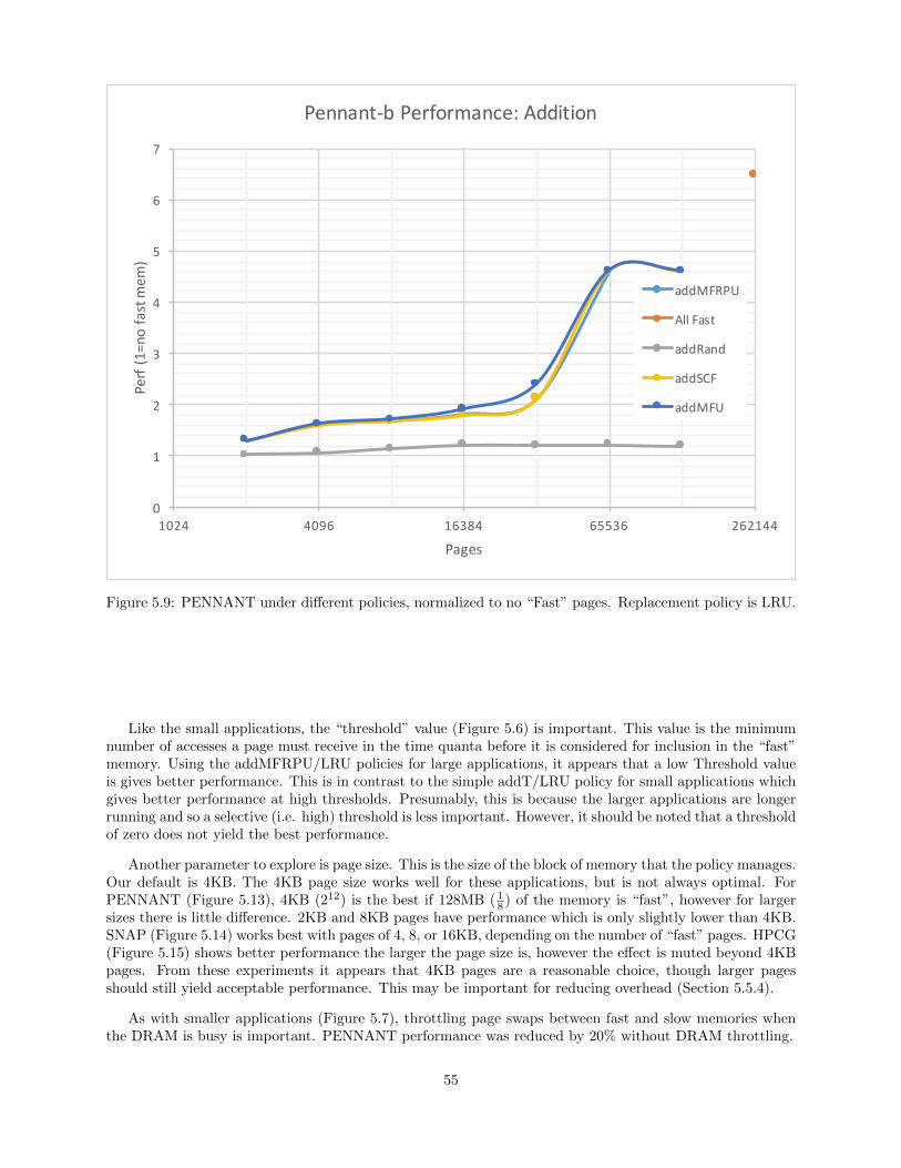
0

1

2

3

4

5

6

7

1024 4096 16384 65536 262144

Perf(1=nofastmem

)

Pages

Pennant-bPerformance:Addition

addMFRPU

AllFast

addRand

addSCF

addMFU

Figure 5.9: PENNANT under different policies, normalized to no “Fast” pages. Replacement policy is LRU.

Like the small applications, the “threshold” value (Figure 5.6) is important. This value is the minimumnumber of accesses a page must receive in the time quanta before it is considered for inclusion in the “fast”memory. Using the addMFRPU/LRU policies for large applications, it appears that a low Threshold valueis gives better performance. This is in contrast to the simple addT/LRU policy for small applications whichgives better performance at high thresholds. Presumably, this is because the larger applications are longerrunning and so a selective (i.e. high) threshold is less important. However, it should be noted that a thresholdof zero does not yield the best performance.

Another parameter to explore is page size. This is the size of the block of memory that the policy manages.Our default is 4KB. The 4KB page size works well for these applications, but is not always optimal. ForPENNANT (Figure 5.13), 4KB (212) is the best if 128MB ( 1

8 ) of the memory is “fast”, however for largersizes there is little difference. 2KB and 8KB pages have performance which is only slightly lower than 4KB.SNAP (Figure 5.14) works best with pages of 4, 8, or 16KB, depending on the number of “fast” pages. HPCG(Figure 5.15) shows better performance the larger the page size is, however the effect is muted beyond 4KBpages. From these experiments it appears that 4KB pages are a reasonable choice, though larger pagesshould still yield acceptable performance. This may be important for reducing overhead (Section 5.5.4).

As with smaller applications (Figure 5.7), throttling page swaps between fast and slow memories whenthe DRAM is busy is important. PENNANT performance was reduced by 20% without DRAM throttling.

55

5.5.3 Cost & Performance

Automatic management of MLM can improve application performance by 20-380% (Figure 5.16) dependingon the application and the amount of “fast” memory. However, MLM comes with added costs. “Fast”memory technologies will almost certainly be more expensive in terms of $ per bit of memory. Additionally,adding extra memory channels or packaging will also impact total system cost.

The exact cost per bit of future memory technologies is difficult to discern, so we examine two scenarios:a cost per bit (relative to DDR) of 1.3× and 5×. Figure 5.17 shows the performance divided by the cost formemory systems with 1

128 th to 12 of their memory comprised of fast memory. In the case where fast memory

is only 30% more expensive than DDR, the curves are substantially similar to the raw performance trends.Marginally improved applications (e.g. SNAP) shows diminishing returns after 1

8 th (32K pages). For the5× case, the trade-off is more pronounced. Adding more than 1

16 th “fast” memory adds more cost thanperformance to PENNANT and HPCG. For SNAP, the overall performance / cost impact is negative – itwould be better to stick with DDR.

5.5.4 Overheads

In addition to the added cost per bit, automatic management also requires additional hardware in theprocessor or memory controller (Section 5.3). The largest component of this hardware would be the SRAMtables required to store the access count information for each page in fast memory.

Conservatively, we estimate that each page in fast memory requires 32 bytes of SRAM storage. Assumingthat SRAM costs 150× per bit as DDR and “fast” memory is 1.3× we can construct a rough cost modelwhich includes overhead (Figure 5.18). This shows that for large “fast” memories and 4K pages, the cost ofSRAM is considerable. Memory systems with lots of fast memory would spend almost as much on SRAMas on main memory.

Dividing the performance by the cost (with overhead) makes large fast memories questionable for lower-performing applications (Figure 5.19. For systems with large amounts of fast memory, manual allocationmay be better.

The high overheads for automatic management may be reduced through a few optimizations. First, pagesizes greater than 4KB would reduce overhead greatly. As shown in Section 5.5.2, many applications continueto perform well with larger page sizes. This could make automatic management of large fast memories moretenable. For example, with 50% of the memory “fast” and 4K pages, SNAP’s performance/cost ratio is 83-92% compared to DDR. However, with 8K pages it is 100-109%. For 16K pages, it is 112-124%. Additionally,the choice of 32KB for the per-page meta-information is conservative. It should be possible to use muchsmaller data structures.

5.5.5 Comparison to Manual Management

We now compare manual and automatic management policies. Note that this comparison comes with animportant caveat – because of the simulation infrastructure available we were unable to use exactly the samearchitecture and simulation models in both studies. For the manual study, we model HMC using GoblinHMCand DRAM using DRAMSim. For the lightweight architecture, we set two of the four memory controllers tobe HMC and two to manage DDR DRAM. In contrast, for automatic we use VaultSim for the HMC modeland DRAMSim for the conventional DRAM. Each of the four memory controllers manages both types ofmemory. As such, the manual management’s system is likely to have higher performance – a less accurateHMC model, increased memory parallelism, and a lower average network latency. Still, the comparison cantell us the likely trend between the policy types.

With that caveat in mind, we plot the performance of the best manual and the best automatic policy in

56

Figure 5.20. As expected, for a given portion of “fast” memory, automatic management generally offers higherperformance than manual management (Figure 5.20). However, looking at the absolute numbers, manualmanagement of HPCG attains only 38.6% of the performance of automatic management for small sizes offast memory ( 1

8 ), though at larger sizes it achieves up to 73.4%. Manually managed SNAP consistentlyachieves greater than 90% of the performance of automatically managed SNAP. Manual PENNANT rangesfrom 40-80% of the performance of automatic management. Because HPCG and PENNANT are especiallysensitive to available memory parallelism, we conclude that the two policy variants likely perform similarly.

Therefore, the costs, benefits, and viability of each policy becomes central. Automatic mangementrequires less programmer effort, but more hardware and a greater capital cost. Manual management on theother hand can require significant programmer investment and so higher labor costs.

57

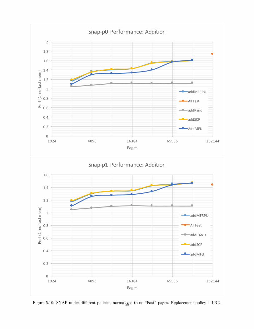
0

0.2

0.4

0.6

0.8

1

1.2

1.4

1.6

1.8

2

1024 4096 16384 65536 262144

Perf(1=nofastmem

)

Pages

Snap-p0 Performance:Addition

addMFRPU

AllFast

addRand

addSCF

AddMFU

0

0.2

0.4

0.6

0.8

1

1.2

1.4

1.6

1024 4096 16384 65536 262144

Perf(1=nofastmem

)

Pages

Snap-p1 Performance:Addition

addMFRPU

AllFast

addRAND

addSCF

addMFU

Figure 5.10: SNAP under different policies, normalized to no “Fast” pages. Replacement policy is LRU.58

0

1

2

3

4

5

6

1024 4096 16384 65536 262144

Perf(1=nofastmem

)

Pages

HPCGPerformance:Addition

addMFRPU

Series2

addRAND

addSCF

addMFU

Figure 5.11: HPCG under different policies, normalized to no “Fast” pages. Replacement policy is LRU.

59

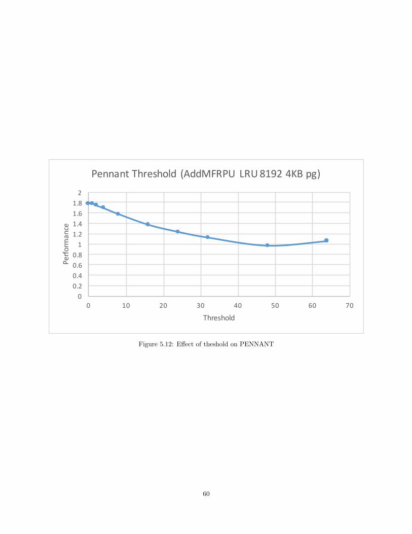
00.20.40.60.81

1.21.41.61.82

0 10 20 30 40 50 60 70

Perfo

rmance

Threshold

PennantThreshold (AddMFRPU LRU81924KBpg)

Figure 5.12: Effect of theshold on PENNANT

60

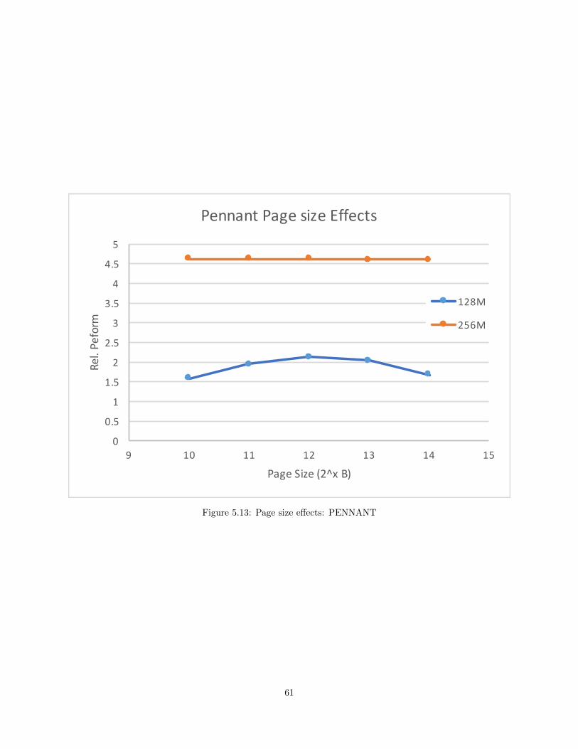
0

0.5

1

1.5

2

2.5

3

3.5

4

4.5

5

9 10 11 12 13 14 15

Rel.Peform

PageSize(2^xB)

PennantPagesizeEffects

128M

256M

Figure 5.13: Page size effects: PENNANT

61

1.46

1.48

1.5

1.52

1.54

1.56

1.58

1.6

9 10 11 12 13 14 15

Rel.Peform

PageSize(2^xB)

snap-p0 PagesizeEffects

128M

256M

1.37

1.38

1.39

1.4

1.41

1.42

1.43

1.44

1.45

1.46

9 10 11 12 13 14 15

Rel.Peform

PageSize(2^xB)

snap-p1 PagesizeEffects

128M

256M

Figure 5.14: Page size effects: SNAP62

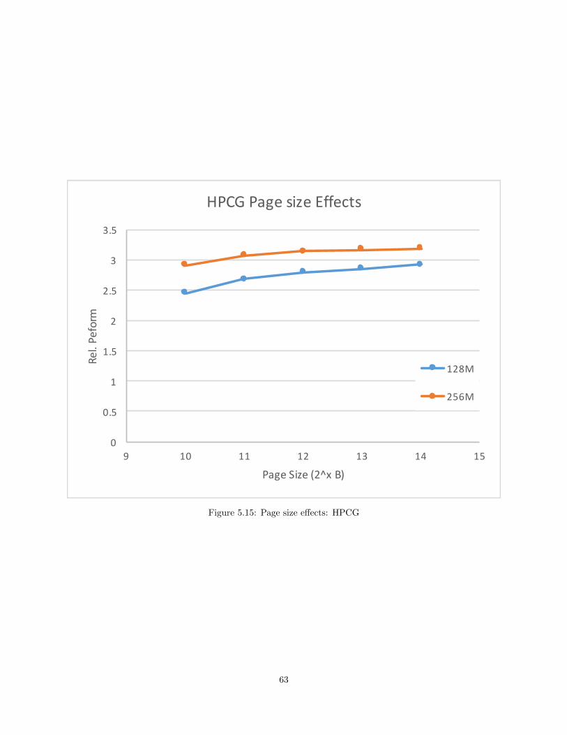
0

0.5

1

1.5

2

2.5

3

3.5

9 10 11 12 13 14 15

Rel.Peform

PageSize(2^xB)

HPCGPagesizeEffects

128M

256M

Figure 5.15: Page size effects: HPCG

63

0

1

2

3

4

5

6

1024 4096 16384 65536

Perfo

rmance

Performancevs.#FastPages

Pennant

snap-p0

snap-p1

Hpcg

Figure 5.16: Large application performance

0.5

1

1.5

2

2.5

1024 4096 16384 65536

Perfo

rmance/Cost

Performance/Costvs#FastPages:Fast5xCost

Pennant

snap-p0

snap-p1

Hpcg

0.5

1

1.5

2

2.5

3

3.5

4

4.5

1024 4096 16384 65536

Perfo

rmance/Cost

Performance/Costvs.#FastPages:Fastx1.3Cost

Pennant

snap-p0

snap-p1

Hpcg

Figure 5.17: Large application performance vs. cost

64

0

0.5

1

1.5

2

2.5

0% 10% 20% 30% 40% 50% 60% 70% 80% 90% 100%

Rel.Cost

%FastMemory

MemorySystemCost

MainMemorySRAMTabelsTotal100%Fast

Figure 5.18: Memory system cost, including SRAM tables

0.5

1

1.5

2

2.5

3

3.5

4

4.5

1024 4096 16384 65536

Perfo

rmance/Cost

Performance/Cost:Fastx1.3,SRAMx150

Pennant

snap-p0

snap-p1

Hpcg

Figure 5.19: Memory system cost / performance

65

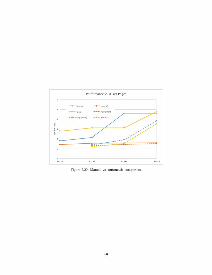
0

1

2

3

4

5

6

16384 32768 65536 131072

Perfo

rmance

Performancevs.#FastPages

Pennant snap-p0

Hpcg Pennant(M)

snap-p0(M) HPCG(M)

Figure 5.20: Manual vs. automatic comparison

66

Chapter 6

Conclusions & Future Work

6.1 Conclusions

The emergence of high-bandwidth memory components has the potential to address the decades old problemof the “memory wall” limiting application performance. Components are available today with up to 5Xprevious bandwidths and into the future even higher improvements will be possible. However, the higherbandwidth comes at higher purchase cost and may be available only in limited capacities. We may thereforebe resigned to seeing higher bandwidth memories as part of a larger node with larger, capacities stores alsobeing provided. Such a drastic change in fundamental node architecture raises some interesting potentialchallenges for our existing high-performance scientific code base.

In this study we have evaluated several aspects to this potential view of the future including applicationperformance in hardware-supported management of resources, operating-system or runtime managementand application/programmer directed. We find an array of impacts on application execution and note thata one-size fits all does not appear to stand out from the results in all cases.

The selection of data structures for placement in high-bandwidth memory was evaluated in this studyand we find that the selection of such allocations is non-intuitive. Programmers seem to understand whichof their data structures will be the “hottest” in access rates but we often find that such intense accesses areabsorbed by a well functioning cache hierarchy. It is therefore a second collection of “less-hot” data structureswhich are the real candidates for high-bandwidth resources. The improvements and new tooling developedwithin SST for this study show a potential path to identifying such allocations for complex memory systemsand architectures that are well beyond those available in the laboratories today.

The assessment of automatic hardware management has also found that one of the most importantindicators of system performance is not what page is selected from replacement but which page is selectedfor addition into a higher-bandwidth resource.

Complex memory hierarchies are clearly challenging our current thinking about application and algorithmdesign. The potential lost performance of mis-calculating what data structures to place where can bedisastrous and therefore it is important that the community has access to scalable and efficient tools andmethodologies to trade off design choices. In this milestone we have extended the SST simulation frameworkto address this challenge. Further, we have validated components within the simulation infrastructure toensure that our findings are based on accurate predictive mechanisms.

As we look to the future the insights of this study stand out – applications are not comprised entirely ofbandwidth bound kernels. Indeed, a variety of bandwidth, latency, and compute boundedness can be seenin our results. For the kernels which are bound by latency, next-generation memory systems will clearlypresent a significant performance challenge making these kernels a potential bottleneck.

67

6.2 Future Work

In this study we have focused uniquely on memory systems comprising of two memory pools but futuredesigns may opt to increase this further. We note that this may include the addition of other levels inthe memory hierarchy such as non-volatile storage which will be slower than DDR and asymmetric forread/write operations. Alternatively, multiple pools of memory may be added introducing greater NUMAor non-uniform performance effects. SST is well positioned as a tool for future studies in this area.

We also intend to evaluate the energy impacts of multi-level memory system design using SST. Since theintroduction of multi-level memory systems can see higher occurrences of data movement it may well be thecase that performance is improved but at the cost of much higher power and energy consumption. Our useof SST statistics gathering will form a basis for this work and seek to answer the question of whether suchan approach can provide gains in energy efficiency.

6.2.1 Manual Management

The results of manual management techniques indicate a clear need for tools to help identify memory regionsor structures for inclusion in different layers of memory. The MemSieve tool is a first cut of such a tool, butrequires extension to become useful to the broader audience of application developers.

We hope to extend MemSieve to make it easier to use and faster. Specifically, automating the workflowand simplifying the interface would allow application developers to use the tool. MemSieve can also be madefaster. An open area for exploration is the size of a memory footprint required to adequately identify keyallocation sites. If it is possible to run an application with a much smaller footprint and still get accurateresults for larger footprint runs, the analysis can be performed much more quickly.

Another area for exploration is a combination of automatic management and programmer hints. Thismay be used to improve performance and/or reduce overhead.

6.2.2 Automatic Management

The current studies show great promise for automatic management of MLM. We hope to expand upon thiswork in several ways.

More detailed modeling of the memory systems and policy overheads will be pursued. This will includeexamining the latency sensitivity of the policy unit to determine if parts of the policy decisions can be madeby the Operating System or runtime instead of hardware.

There are many chances to optimize policies and policy parameters. It may be possible to auto-tunepolicy parameters or to dynamically select policies. There are also possibilities for programmer or compilerfeedback to guide policies.

The current implementation does not allow accesses to pages that are being transferred between differentlayers of memory. This can delay a sizable fraction of accesses (up to 8% for CoMD addSC/LRU). A moreadvanced Policy Dispatcher in the MLM Unit may be able to be less restrictive and allow access to pageswhich are only partially transfered.

Reducing the hardware overhead of automatic management is critical for many applications and memorysizes. We will explore larger page sizes, reducing the size of meta-data structures, and compression or cachingof data structures.

68

6.3 Recommendations

Finally, we conclude this report with a summary of the recommendations gleaned from the different analysesperformed. For architectural and system design our recommendations are:

• Latency should not be sacrificed for bandwidth (Section 3.3)

• Consideration for the management policy must be part of any architectural trade-off study

• Applications vary widely in their ability to use higher bandwidth, but in general a moderate-to-smallHMC-to-DRAM ratio should be sufficient

• An HMC/HBM is not a conventional cache (higher bandwidth but not lower latency) so conventionalcaching policies do not perform well

• For management, we recommend that either a hardware/automatic approach be taken or that theOS/runtime manage MLM with the ability to leverage memory usage information provided by theapplication (“hints”)

For applications we make the following recommendations:

• Use data pools or other techniques to avoid many small calls to malloc

• Very large allocations may be hard to manage efficiently if managing at a malloc granularity

• Try to create program phases (i.e., a particular computation or threaded section) whose memoryfootprint fits in the fast memory. This will benefit both automatic and manual management policies.

• An API to enable application writers to manage allocations within libraries is needed

• Tools such as MemSieve will be instrumental for enabling applications to get better performance outof MLM systems

• The best allocations for HMC/HBM are those that are accessed frequently but not so frequently theyend up in the cache. Identifying such allocations is not always intuitive.

69

70

References

[1] Michael A. Bender, Jonathan W. Berry, Simon D. Hammond, K. Scott Hemmert, Samuel McCauley,Branden Moore, Benjamin Moseley, Cynthia A. Phillips, David S. Resnick, and Arun Rodrigues. Two-level main memory co-design: Multi-threaded algorithmic primitives, analysis, and simulation. In 2015IEEE International Parallel and Distributed Processing Symposium, IPDPS 2015, Hyderabad, India,May 25-29, 2015, pages 835–846, 2015.

[2] MT Bettencourt. MiniPIC - A Particle-In-Cell (PIC) Code on Unstructured Grids for Next GenerationPlatforms. In 2015 IEEE International Conference on Plasma Sciences (ICOPS), pages 1–1. IEEE,2015.

[3] Z. Chen, N. Xiao, F. Liu, and Y. Zhao. Ssarc: The short-sighted adaptive replacement cache. In HighPerformance Computing and Communications, 2009. HPCC ’09. 11th IEEE International Conferenceon, pages 551–556, June 2009.

[4] J. Dongarra, M. Heroux, and P. Luszczek. Hpcg benchmark: A new metric for ranking high performancecomputing systems. Technical Report UT-EECS-15-736, ECE Department, University of Tennessee,Knoxville, TN, 2015.

[5] C. R. Ferenbaugh. Pennant: an unstructured mesh mini-app for advanced architecture research. Con-currency and Computation: Practice and Experience, 27(17):4555–4572, 2015.

[6] Michael A Heroux, Douglas W Doerfler, Paul S Crozier, James M Willenbring, H Carter Edwards,Alan Williams, Mahesh Rajan, Eric R Keiter, Heidi K Thornquist, and Robert W Numrich. ImprovingPerformance via Mini-Applications. Technical Report SAND2009-5574, Sandia National Laboratories,2009.

[7] Bruce Jacob, Spencer Ng, and David Wang. Memory Systems: Cache, DRAM, Disk, chapter Overviewof DRAMS, pages 315–341. Morgan Kaufmann, 2008.

[8] Jagan Jayaraj, Arun F. Rodrigues, Simon D. Hammond, and Gwendolyn R. Voskuilen. The potentialand perils of multi-level memory. In Proceedings of the 2015 International Symposium on MemorySystems, MEMSYS 2015, Washington DC, DC, USA, October 5-8, 2015, pages 191–196, 2015.

[9] Theodore Johnson and Dennis Shasha. 2q: A low overhead high performance buffer managementreplacement algorithm. In Proceedings of the 20th International Conference on Very Large Data Bases,VLDB ’94, pages 439–450, San Francisco, CA, USA, 1994. Morgan Kaufmann Publishers Inc.

[10] Ian Karlin, Jeff Keasler, and Rob Neely. Lulesh 2.0 updates and changes. Technical Report LLNL-TR-641973, LLNL, August 2013.

[11] Chi-Keung Luk, Robert Cohn, Robert Muth, Harish Patil, Artur Klauser, Geoff Lowney, Steven Wallace,Vijay Janapa Reddi, and Kim Hazelwood. Pin: Building Customized Program Analysis Tools withDynamic Instrumentation. In ACM Sigplan Notices, volume 40, pages 190–200. ACM, 2005.

[12] M. Pavlovic, N. Puzovic, and A. Ramirez. Data placement in hpc architectures with heterogeneousoff-chip memory. In Computer Design (ICCD), 2013 IEEE 31st International Conference on, pages193–200, Oct 2013.

[13] Steve Plimpton. Fast Parallel Algorithms for Short-Range Molecular Dynamics. Journal of Computa-tional Physics, 117(1):1 – 19, 1995.

[14] Steve Plimpton. LAMMPS Molecular Dynamics Simulator. http://lammps.sandia.gov, March 2016.

71

[15] A. F. Rodrigues, K. S. Hemmert, B. W. Barret, C. Kersey, R. Oldfield, M. Weston, R. Risen, J. Cook,P. Rosenfeld, E. CooperBalls, and B. Jacob. The structural simulation toolkit. SIGMETRICS Perform.Eval. Rev., 38(4):37–42, 2011.

[16] ChunYi Su, David Roberts, Edgar A. Leon, Kirk W. Cameron, Bronis R. de Supinski, Gabriel H. Loh,and Dimitrios S. Nikolopoulos. Hpmc: An energy-aware management system of multi-level memoryarchitectures. In Proceedings of the 2015 International Symposium on Memory Systems, MEMSYS ’15,pages 167–178, New York, NY, USA, 2015. ACM.

[17] Kshitij Sudan, Anirudh Badam, and David Nellans. NAND-Flash: Fast Storage or Slow Memory?Technical report, University of Utah, 2012.

[18] J. Zerr and R. Baker. SNAP: SN (Discrete Ordinates) Application Proxy, Version 1.07. TechnicalReport LA-CC-13-016, Los Alamos National Laboratory, New Mexico, USA, 2016.

72

DISTRIBUTION:

1 MS 0845 M.W. Glass, 01545

1 MS 1319 J.A. Ang, 01421

1 MS 1319 K.S. Hemmert, 01422

1 MS 1319 J.H. Laros, 01422

1 MS 1319 S.D. Hammond, 01422

1 MS 1319 G.R. Voskuilen, 01422

1 MS 1319 A.F. Rodrigues, 01422

1 MS 1319 R.J. Hoekstra, 01422

1 MS 1319 M.P. Frank, 01425

1 MS 1319 J. Aidun, 01425

1 MS 1319 M.A. Heroux, 01426

1 MS 1322 K.F. Alvin, 01420

1 MS 0899 Technical Library, 9536 (electronic copy)

73

74

v1.37