1

Evaluating the impact of land redistribution: A CGE microsimulation application to Zimbabwe1

Margaret Chitiga*a, Ramos Mabugub

a Department of Economics, University of Pretoria, Pretoria 0002, South Africa

b Financial and Fiscal Commission, Midrand, South Africa

Zimbabwe has recently gone through a widely criticised land reform process. The country has suffered immensely as a result of this badly orchestrated reform process. Yet land reform can potentially increase average incomes, improve income distribution and as a consequence reduce poverty. This paper presents a counterfactual picture of what could have happened had land reform been handled differently. The paper uses a computable general equilibrium (CGE) model coupled with a microsimulation model in order to quantify the impact of land redistribution in terms of poverty, inequality and production. This is to our knowledge the first attempt to apply such an approach to the study of the impact of land reform on poverty and distribution in the context of an African country. The results for the land reform simulations show that the reform could have had the potential of generating substantial reductions in poverty and inequality in the rural areas. The well off households, however, would have seen a slight reduction in their welfare. What underpins these positive outcomes are the complementary adjustments in the fiscal deficit and external balance, elements that were generally lacking from the way Zimbabwe’s land reform was actually executed. These results tend to suggest that well planned and executed land reforms can still play an important role in reducing poverty and inequality.

JEL Classification: D31, D63, D58, Q15 Keywords: Computable General Equilibrium, Land reform, Microsimulation, Poverty,

Inequality.

1. Introduction

1 This work was carried out with the model built from a grant from the Poverty and Economic Policy (PEP) Research Network (www.pep-net.org), financed by the International Development Research Centre (IDRC). We received intensive data and technical assistance on the original work from Professors Bernard Decaluwe and John Cockburn, Dr Nabil Annabi and Mr. Ismael Fofana. Suggestions from an anonymous referee and the managing editor of this journal are gratefully acknowledged. Any errors remain our own.

* Corresponding author. Tel.: +27 12 4203457; fax: +27 12 3625207 Email address: margaret.chitiga@.up.ac.za.

2

There are many authors that argue that land redistribution is good for growth (Birdsall and

Londono (1997), Burgess and Beasly (1998), Deninger and Squire (1998) and Aghion

(1999)). The World Development Report of 2001 argued that lower growth could be caused

by inequality in the land ownership distribution (World Bank (2001)). Deninger et al (2000)

show that land redistribution can reduce poverty and because it increases efficiency, it will

lead to growth. The end of the 1990s marked the beginning of an era of deep and

controversial land reforms in Zimbabwe. The government redistributed a substantial amount

of the land owned by white farmers to black farmers in a very short time span in what has

now come to be known as the fast track land reform. Prior to the fast track land reform, the

“willing-seller-willing-buyer” principle directed government land reform. Given the slowness

of the redistribution process achieved under the “willing-seller-willing-buyer” principle as

well as the costs involved, the authorities revised their timescale and embarked on the fast

track land reform. Contrary to the optimism found in the literature cited above concerning the

benefits of land reform, the outcome for Zimbabwe has been dismal. Poverty rates and

inequality have gone up substantially following the land reform. Far from hurting only

commercial farmers who have lost farms, the economic decline has had widespread negative

effects on the general population. Does this mean that Zimbabwe provides evidence that does

not support most of the studies predicting beneficial impacts of land reform or could the

mismanagement of the land reform process have contributed to the increase in poverty that is

now associated with land reform?

There are a growing number of studies that have emphasized the political economy aspects of

the Zimbabwean land reform. For instance, Moyo and Yeros (2004) argue that the land

reform is an instance similar to a national democratic revolution while Davies (2004) argues

that the reform has destroyed rather than created capital and has weakened the revolution.

Zimconsult (2004) argues that poor planning and government’s failure to move to restoring

food security are not the only problems but also its use of food as a political weapon has

negatively contributed to the outcome. As would be expected, there are no tangible data with

which to evaluate these arguments so that emotions and confusion have surrounded this

debate. Rather than continue with the debate along these lines, this paper reassesses the land

reform programme in Zimbabwe with a particular focus on some very interesting economic

questions that were largely ignored in the way the programme was executed and in the

normal discourse over the effects of land reform.

3

This paper intends to make two contributions to the literature on land reforms in Africa.

Firstly, to make sense of the economic decline that has ensued in Zimbabwe, it would appear

that the relevant question is what the outcome would have been had the government seriously

committed to credible macroeconomic policies while carrying out the land reform exercise.

This is a hypothetical question in the sense that the land reform program was administered in

an atmosphere of high and growing macroeconomic imbalances and therefore requires the

construction of a relevant counterfactual. There is likely to be disagreement over the relevant

counterfactual. To increase transparency, the issue of a counterfactual is handled in this paper

by constructing a model that assumes the maintenance of the pre-crisis macroeconomic

structure. Secondly, drawing on recent poverty modelling literature, the paper presents a

relatively new paradigm for analyzing the poverty impacts of land reforms in African

economies. The insights from this literature are incorporated into a separate generic

microsimulation model that is linked to a computable general equilibrium (CGE) model. The

CGE model coupled with a microsimulation model is then used to quantify the impact of land

redistribution in terms of poverty, inequality and production. Recent work in the CGE

tradition that explores the consequences of land reform for Zimbabwe include the work of

Bautista et al (1998, 2000), while Juana and Mabugu (2005) explore a similar issue using a

Social Accounting Matrix (SAM) multiplier approach. The value added of the work carried

out in this paper lies in the explicit poverty modelling accomplished through the use of

microsimulation techniques linked to a CGE model. There is no parallel work in Zimbabwe

and indeed in the rest of Africa that we are aware of that has applied this technique to land

reform issues.2

The rest of the paper is arranged as follows: section 2 briefly discusses the issues surrounding

land reform in Zimbabwe while section 3 presents the model. Section 4 discusses the

simulation implemented as well as the results. Section 5 concludes the paper.

2. Background to land issues in Zimbabwe

Zimbabwe inherited a prosperous agro-based economy at independence in 1980. However,

the agricultural sector was dual in nature with the coexistence of a large-scale commercial

(LSC) sector controlled by mainly white farmers, and a small-scale communal agricultural

2 For recent microsimulation CGE models applied to trade issues, see for example Cockburn (2001) and Cororaton (2003).

4

sector owned by the indigenous African people. Small scale agriculture was further divided

into small scale commercial agriculture and communal agriculture. After independence,

another sector consisting of resettled farmers was formed within the small scale agriculture

sector. Although white farmers made up less than one per cent of the population, they

controlled more than half of the productive land. Small scale farmers tended to practice

mixed cropping of mainly non-export oriented crops and tended to use their land more

intensively than large scale commercial farmers. Chiremba and Masters (2003) report the

national-average cropping intensity of 1994 as 4 per cent for large scale commercial farmers,

11 per cent for communal farmers and 8 per cent for resettled farmers.

From the outset, Zimbabwe pursued a land acquisition strategy based on a ‘willing-seller-

willing-buyer’ principle along the lines agreed at the Lancaster House in 1979 during the

country’s independence negotiations. The government was the main buyer, having received

grants approximately equal to US$44 million during the 1980s from Britain for land

acquisition (Moyo (2004)). About 430,000 hectares were acquired each year between 1980

and 1986, falling to an average acquisition of 75,000 hectares per annum between 1985 and

1992 and approximately 158,000 hectares per year between 1992 and 1997 (Moyo (2004)).

The acquired land was given to about 70,000 families against a target of 162,000 families for

resettlement while white settler farmers land ownership had fallen from 50 per cent of

agricultural land in 1980 to 29 per cent in 1986 (Moyo (1995)). The Lancaster House

constitutional safeguards for market-based land transfers expired in 1990.

Starting in 1997 and largely led by war veterans, land seizures began. Government responded

by formalizing the seizures in what came to be known as the compulsory land acquisition

law, which was the defacto successor to the ‘willing-seller-willing-buyer’ principle. Another

important development was the collapse of ongoing discussions over land reform between the

government and the United Nations Development Program and the British Government in

2000 as this signaled the end of any hopes for a negotiated solution to the land crisis. The

government announced that it would repossess 1471 commercial farms, which translated to

more than 11 million hectares of land. This makes up about 40 per cent of the total

commercial land (OECD (2003)). According to Moyo (2004), smallholder farmers’ control of

land had increased to 70 per cent of the land by 2003 while the area designated as

commercial experienced a 42 per cent drop in land area.

5

Before the onset of the fast track land reform, the agricultural sector employed a total of over

70 per cent of the labour force (Christiansen (1993)). Agriculture contributed between 9 per

cent and 15 per cent to gross domestic product (GDP) and between 20 per cent and 33 per

cent to export earnings. The sector was an important supplier of raw materials to the

industrial sector, contributing 20 per cent of the manufacturing inputs in the eighties.

What has happened since then in terms of the economy is nothing short of a catastrophe. Real

GDP growth has been negative since 2000, reaching –14.5 per cent in 2002, and projected at

–12.4 per cent for 2003 (Matshe (2004)). According to Davies (2004), real income per head

in 2004 was projected to be 46 per cent less than it was in 1996 based on government official

data or 53 per cent less if data from the International Monetary Fund were used. According to

CIA (2007), the population below the poverty line was estimated at 80 per cent in 2004,

while the Gini index was estimated at 56.8 for 2003. These statistics are markedly higher than

those reported in CIA (1998) showing that the population below the poverty line was

estimated to be 25.5 per cent between 1990 and 1991. CIA (2004) reported that the

population below the poverty line was estimated at 70 per cent in 2002 and the Gini index

was 50.1 for 1995. These statistics show that poverty and inequality increased substantially

between the period 1990 and 2004. Chitiga and Mabugu (2005) report that poverty levels

have likely continued to rise since 2000, largely driven by the dismal macroeconomic

performance, drying up of important external aid inflows and high inflation (largely a result

of supply shortages (due in part to reduced agricultural farming activity and droughts) and

huge budget deficits)). Given the high inflation rates that have characterized the economy

since 1997 and the massive job losses, it is not surprising that income distribution has not

improved during the period.

It is not easy to isolate and quantify the effects of the fast track land reform because of the

many interactions that took place (for example weather, international “sanctions”, governance

and bad economic policies and outcomes). There is need to develop a picture of what could

have happened had land reform been carried out without these disturbances. The argument

that is explored in this paper is based on a counterfactual and is premised on a contention that

such suffering as was experienced in Zimbabwe could have been avoided had the land reform

been done with due care being taken of the consequences for the fiscal and external deficit as

well as other external shocks.

6

3. Empirical modelling framework

This paper uses a Walrasian CGE model to present a counterfactual picture of what could

have happened to the Zimbabwean economy following a well-executed land reform. The

model is based on the EXTER+ model (see Decaluwé et al (1999), Cockburn and Cloutier

(2002) and Cockburn et al (2004)).3 The focus is on the effects on poverty and inequality.

The model is implemented using benchmark data from 1995, a date by which the fast track

land reform had clearly not commenced. The details of the SAM are documented in Chitiga

et al (2000). The year 1995 is arguably the last stable benchmark for the economy before the

onset of the fast track land reform exercise and also coincides with available data from a

household survey. For these reasons, 1995 was considered to be a suitable benchmark.

The model has 16 production sectors and activities. These are grain crops, horticulture crops,

tea and coffee, cotton and tobacco, all other crops, livestock, fishery, forestry, mining, food

processing, textile, all other manufacturing, construction, water, electricity and other trade

services, public services and all other private services. Half of the sectors are agricultural

based since the emphasis of the paper is on agricultural land. Typical to most other CGE

models, the model does not distinguish production functions by household or farming group

but according to sectors. Each sector’s output is homogeneous. Assuming different

production functions by type of farmer would require very detailed information on household

production technology based on survey of production and would entail introducing

heterogeneity at the producer level. This way of modelling production is not pursued in this

paper because we do not have at our disposal a detailed production survey for the base year

for the Zimbabwe model. There are 4 factors of production, namely, skilled labour, unskilled

labour, capital and land. The sequential micro-model incorporates 14006 households. These

households’ incomes and expenditures are derived from the 1995 Poverty Assessment Study

Survey (PASS) (Government of Zimbabwe 1996).

The model makes use of multi level nested production functions to determine production.

Sectoral output is a Leontief combination of intermediate consumption and value added.

Similarly, intermediate demand by sectors is modeled using Leontief functions. Value added

is modelled as a constant elasticity of substitution (CES) aggregation of capital and labour. In

3 Some of the published CGE evaluations applied to Zimbabwe include Davies et al (1994, 1998), Rattsø and Torvik (1998), Chitiga (2000) and Mabugu (2001).

7

the agricultural sector, land is included in the CES function between the composite factor

(capital and labour) and land. The model distinguishes two labour categories of skilled and

unskilled labour types and specifies a CES function to capture the relationship between them.

It is assumed that there are given factor endowments. Capital and labour are freely mobile

across the sectors so that wages for each skill type and return on capital are the adjusting

variables clearing the capital and labour markets.

Next it is assumed that there are four types of institutions corresponding to households,

government, firms and the rest of the world. The CGE model contains five household groups

divided according to their labour use, their farming structure and whether they are urban or

rural based. The five household types are as follows: communal farmers, commercial farmers

(who include large scale and small scale farmers), farm workers, urban unskilled income

earners and urban skilled income earners. The first two groups are rural based, derive a large

part of their income from land and are assumed to be the only land owners in the model. The

third group is also rural based and derives most of its income from unskilled employment

supplied at the farms. The last two groups are urban based, the fourth one deriving its main

labour income from unskilled employment and the fifth from skilled employment. In

addition, households can also earn income from capital and transfers from each other, from

the rest of the world and from the government. Capital pays mainly the urban skilled income

earners and the rural commercial farmers. Commercial farmers in addition also derive

substantial income from skilled employment. This is income earned by farm owners who are

usually also farm managers. These five types of households are representative of the micro-

model in which all households from a survey are included. We thus map the results from the

CGE model to the micro model after a simulation according to the group in which each

household belongs. This micro-model distinguishes 14006 households that fit into one of each

of the five household groups.

Table 1 shows the factor income shares of the different households. They spend their income

on payment of taxes, transfers to other institutions and savings to remain with disposable

income. The households allocate their disposable income to sectoral consumption by

maximising a Stone Geary type utility function taking prices as given. It is assumed that

household savings propensities are fixed and calibrated from the SAM data. Savings levels

8

will vary with the level of economic activity. Enterprises receive income from capital and

transfers from other institutions. They pay taxes, save and transfer income to other

institutions but do not consume sectoral output. The government receives direct and indirect

taxes and spends on sectoral consumption, savings and certain transfers. All transfers to

households are fixed in nominal terms. The government expenditure is fixed and a

compensatory tax by means of a direct tax is instituted. This tax adjustment handles any

adjustments required to restore government revenues following a policy shock to ensure that

a given government fiscal balance is achieved.

Table 1: Households endowment income shares in base year

Endowment income source Household type unskilled labour skilled labour capital land Firm Communal farmers 27.2% 0.0% 15.3% 29.5% 0.0% Farm workers 3.3% 0.0% 0.0% 0.0% 0.0% Commercial farmers 0.0% 8.8% 77.3% 70.5% 62.6% Urban unskilled households 69.4% 0.0% 7.4% 0.0% 0.0% Urban skilled households 0.0% 91.2% 0.0% 0.0% 37.4% Total 100% 100% 100% 100% 100%

Sectoral output is sold domestically or abroad. There is imperfect substitution between the

export good and the domestic good. This imperfection is formulated using a constant

elasticity of transformation (CET) specification. Similarly, there is imperfect substitution

between the domestic good and imported goods modelled as a CES specification following

Armington (1969). Imperfect substitutability allows for the existence of two-way trade in the

same commodity as well as giving some measure of independence from external forces to

domestic prices.

Model closure rules refer to macroeconomic adjustments in the model. The choice of closure

rules has a huge influence on the results and as such they should be chosen with due care. We

assume that the government budget deficit and volume of government current consumption

are both fixed. A uniform change in household income tax and company tax rates ensures that

government revenues adjust until the given budget deficit is attained. The assumption that the

budget deficit is fixed ensures that the land reform is not financed simply by larger budget

deficits. We also assume that the current account balance of payments is fixed so that the real

exchange rate is the adjustment variable. Again this assumption is interpreted to mean that

the land reform exercise is not financed by exogenous foreign currency inflows, which

9

accords well with the observation that international aid ground to an almost complete halt

during the fast track land reform. If it is intended that there will be such an inflow, either

through aid or foreign investment, it would be possible to adjust the fixed foreign deficit to

the anticipated amount. The assumption of fixed investment with variable savings helps us to

rule out ‘free lunch’ outcomes where investment can be run down even to negative levels

without there being any negative impact on welfare. Taken together, these closures are in line

with those found in the Zimbabwean CGE literature (see for example Davies et al (1994),

Chitiga and Mabugu (2005) and Bautista et al (1998) and they imply that our modelled

counterfactual is very different to how the government chose to implement fiscal and trade

policy during the fast track land reform exercise. The model is square in the sense that the

number of equations is equal to the number of variables. The model was checked to verify

that it is homogeneous of degree zero in prices. The nominal exchange rate is taken as the

numéraire.

4. Simulation results

The paper simulates a land transfer of 40 per cent from commercial farmers to communal

farmers. The total arable land is maintained at the same level as in the base year. This is very

close to the actual shock that took place during the fast track land reform that started after

1997. To focus on the underlying resource allocation, poverty and macroeconomic issues,

problems of mismanagement or wastage of land are assumed away.

Assuming that the land reform is well managed and targeted in this way, the land reform

generates a significant increase in crops grown by communal farmers. Grain increases by 3.4

per cent compared to its base year value while horticultural crops such as beans and other

vegetables increase by 1.5 per cent. Other crops and livestock also increase as does forestry.

The main reason for the increase in these crops is due to increased demand by communal

households whose incomes have increased. Communal farmers demand the majority of non

export-oriented agricultural products whose supply is increasing.4 There is, on the other hand,

a fall in the agricultural production of cotton and tobacco (0.5 per cent) and tea and coffee

(0.4 per cent). The reason for this decline is because factors are pulled towards the production

4 The SAM data includes formal and informal activities. In the case of forestry, note further that firewood and other forestry services such as fruit and herb collection are included. Communal farmers are the largest demanders of forestry product as a final commodity.

10

of crops grown intensively by communal farmers and demanded by communal farmers and

away from the export crops that are traditionally grown by the commercial farmers. As this

expansion in agriculture takes place, it raises the economywide prices of factors of

production. This increase in production costs hurts mildly the manufacturing and services

sectors. Compounding this effect as well is that the falling agriculture sectors, particularly

cotton, are the major input suppliers to the manufacturing sectors. Figure 1 shows the sectoral

output changes of the land reform intervention.

Figure 1: Sectoral change in output

-1

-0.5

0

0.5

1

1.5

2

2.5

3

3.5

4

Grain

Horticulture

tea&coffee

cotton&tobacco

othercrops

livestock

Fishery

Forestry

mining

fodprocessing

Textile

allothmaufactring

construction

electri,water,transpt

publicservice

privateservice

Change in output

There is a fall in the total exports. This is mainly because the main export crops (tobacco,

cotton, tea and coffee) are the direct casualties of the reform exercise. Coupled with this is the

real exchange rate appreciation brought about by the increase in the consumer price index.

The consequent fall in export revenues leads to a fall in the imports of commodities (the ‘no

free lunch’ condition implied by the closure rules). With falling supply in the main domestic

market (manufacturing and services), all prices increase on the local market. The consumer

price index increases for all households. The return to land improves in the whole economy

while the return to capital falls. Although more capital is attracted in the sectors that are

gaining, much more is shed off in the rest of the economy including the industrial sectors.

The increase in agriculture by non-export sectors attracts more unskilled labour and their

wages increase by 0.6 per cent. The fall in output and the increase in unskilled wage in turn

11

lead to a fall in demand for unskilled labour in the industrial sectors. At the same time, the

reduction in output in the industrial sectors leads to reduced demand for skilled labour,

forcing its wage to fall by 0.2 per cent. The incomes of the communal farmers, (the

beneficiaries of the land reform), increases substantially by about 8 per cent. As expected, the

income of the commercial farmers falls but only by 1.7 per cent. This is because the initial

land income to commercial farmers was far larger than that of communal farmers as seen in

Table 1. Because of the increase in unskilled labour demand, all unskilled workers experience

income increases. The farm workers experience an increase of 0.6 per cent and those

unskilled income households in the urban areas experience gains of 0.5 per cent. The total

income increases are not the same for all unskilled income earners even though there is free

mobility of unskilled workers, which implies that unskilled wage rates are the same in

equilibrium. This is because incomes for each group are influenced by other factors of

production as well as different transfers so that initial factor shares in income play an

important role. For instance, the income of urban unskilled households is additionally

affected by capital income while that of farm workers is only affected by unskilled labour

income. The initial income sources are affected differently for individual groups hence the

different final income changes for each group.

The urban skilled income households who rely on capital and skilled labour income

experience a fall in incomes of 0.2 per cent. There is also another, more subtle

macroeconomic adjustment that is responsible for depressing incomes of the higher-income

groups. Because of reduced economic activity, general tax revenue declines in the economy.

However, because of the way the model is closed, there is an automatic compensation of lost

revenue through increases in direct taxes, which fall disproportionately more on high-income

households. Thus, skilled income earners and the commercial farm households are

responsible for shouldering the burden imposed by the land reform on the fiscal deficit in the

counterfactual.

To discuss the welfare effects of the intervention, use is made of the equivalent variation (EV)

concept. It is used to measure social welfare by comparing the utility of households at price

and income in a reference situation to the utility in the new situation (see Varian 1992).

Equivalent variation is defined as:

1. )( 01

1

12

02

11

01 YMYM

P

P

P

PEV

12

where P1

0: price of good 1 in the base year (before simulation); P1

1: price of good 1 in year 1 (after simulation); P2

0: price of good 2 in the base year (before simulation); P2

1: price of good 2 in year 1 (after simulation); and: YM0: Household income in the base year (before simulation); YM1: Household income in year 1 (after simulation). If: EV>0 increase in household welfare;

EV<0 decrease in household welfare;

Table 2 shows that the communal farmers, farm workers and the urban unskilled households

experience an increase in their welfare following a land reform. The other two households,

however, see a fall in their welfare. Hence, the land redistribution is potentially pro-poor

irrespective of the region where the poor reside.

Table 2: Welfare outcomes (per cent changes)

Communal

farmers Farm

workersCommercial

farmers

Urban Unskilled

households

Urban Skilled

households

Change in disposal income 7.8 0.6 -1.7 0.5 -0.2 Change in total consumption 7.8 0.6 -1.7 0.5 -0.2 Change in household consumer price 0.3 0.3 0.2 0.2 0.1 Equivalent variation 7.1 0.2 -1.4 0.2 -0.2

With the aid of sequential microsimulation techniques, we are able to tell the extent of the

change in poverty and inequality that occurs due to the 40 per cent land redistribution

experiment. Using the new income, consumption and price changes from the CGE model for

the five household types, we adjust each household in the microsimulation model’s

benchmark variables. These new variables are then used to compute poverty indicators using

the Foster, Greer and Thorbecke (FGT) (1984) measures.5

5Poverty is decomposed into the poverty headcount (population below the poverty line), poverty gap and the

severity of poverty. The FGT index is defined as:

q

i

i

z

yz

nP

1

1

Where z is the poverty line, iy is income for household i, n is the total population, q is the number of the poor

population and α is the degree of aversion to poverty. The poverty and inequality measures are computed using the software called DAD that was developed by Duclos et al (2002).

13

The poverty headcount index gives the number of households below the poverty line divided

by the total households in the group when the degree of aversion to poverty is zero. This

shows the prevalence of poverty but does not give a good idea about the degree of poverty.

Poverty depth informs on the mean shortfall of the poor’s income below the poverty line. In

this case the degree of aversion to poverty is set to unity and this enables calculation of the

level of income transfer needed to bring all poor households to the poverty line. Lastly, a

poverty severity index is computed that takes into account the inequality among households

that are poor. In this case, the degree of aversion to poverty is set at two, meaning that more

importance is accorded to the shortfalls of the poorest households. The weight assigned to

each household is equal to its shortfall from the poverty line (see also Ravallion (1994)).

The poverty results are reported in Tables 3 and 4 in terms of the poverty gap, head count

ratio and the poverty severity for each of the household types as well as for the whole

economy. The poverty line used is the national total consumption poverty line of Z$1912.41

in 1995 dollars (approximately USD232) as calculated by the PASS study (Government of

Zimbabwe 1996). This policy leads to an overall decrease in poverty in the economy. This is

the case for all FGT indices showing headcount ratios, the poverty gap and the poverty

severity. The reduction in poverty in the country, however, is coming from the benefits

accruing mainly to rural communities as a result of the land reform. This is because rural

poverty falls substantially. Urban head count poverty slightly increases with the poverty gap

and severity remaining essentially the same.

Table 3: Poverty results for the whole economy and for urban and rural areas

Before simulation

After simulation

Change (per cent)

head count 0.507 0.500 -1.4 (0.00499) (0.00499) Poverty gap 0.245 0.241 -1.6 (0.00299) (0.00297) Poverty severity 0.149 0.146 -2.1

All

(0.00226) (0.00224) head count 0.535 0.525 -1.9 (0.00615) (0.00616) Poverty gap 0.257 0.251 -2.3 (0.00370) (0.00370)

Rural areas

Poverty severity 0.155 0.151 -2.6

14

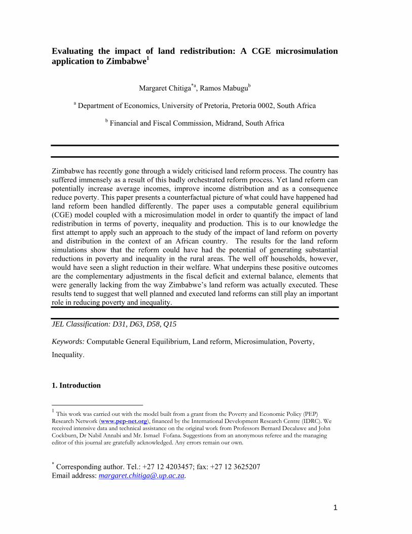
(0.00281) (0.00277) head count 0.443 0.444 0.2 (0.00838) (0.00838) Poverty gap 0.219 0.219 0.0 (0.00498) (0.00498) Poverty severity 0.135 0.135 0.0

Urban areas

(0.00349) (0.00374) Numbers in brackets are standard deviations

Table 4 gives the results for the individual groups. In the case of specific households, poverty

falls for the households that get the land transfer (communal farmers) and increases for those

who have their land reduced (the commercial farmers). This is the case for these two

household groups in terms of the three FGT indices used. It is important to note that the

communal farmers are the poorest group in the model. For farm workers the results are mild.

Poverty gap and severity are reduced but the head count remains essentially the same. The

urban unskilled households are also very slightly affected in terms of poverty reduction. The

increase in income for these two groups is almost eroded by the increase in consumer prices

resulting from lower industrial and services output so that there is a negligible impact on

poverty. It must be pointed out that the poverty result for this group could have been worse

had we assumed no mobility of factors of production between the rural and the urban sectors,

as would be the case in the very short run. This would have meant that the benefits of

increased unskilled labour demand and wages occurring due to the agricultural sector

expansion would not have benefited urban unskilled workers. The assumptions in this model

allows for a medium to long run interpretation of the outcomes. The urban skilled households

experience an increase in poverty. This is mainly brought about in the model by the falling

capital income, the increased direct tax bill required to compensate for government revenue

shortfalls as well as the increasing consumer prices.

Table 4 Poverty results for the different groups

Before simulation

After simulation

Change (per cent)

head count 0.552 0.520 -5.8 (0.00924) (0.00923) poverty gap 0.270 0.2486 -8.3 (0.00552) (0.00537)

Communal farmers

poverty severity 0.165 0.150 -9.2

15

(0.00420) (0.00411) head count 0.627 0.630 0.0 (0.08627) (0.08627) poverty gap 0.293 0.292 -0.3 (0.05039) (0.05035) poverty severity 0.173 0.173 -0.4

Farm workers

(0.04209) (0.04206) head count 0.440 0.446 1.2 (0.00980) (0.00981) poverty gap 0.208 0.212 1.9 (0.00691) (0.00610) poverty severity 0.124 0.127 2.6

Commercial farmers

(0.00399) (0.00412)

head count 0.470 0.470 0.0 (0.01319) (0.013191) poverty gap 0.230 0.230 0.0 (0.00800) (0.00800) poverty severity 0.146 0.146 -0.4

Urban unskilled households

(0.00605) (0.00604) head count 0.423 0.425 0.5 (0.01070) (0.01070) poverty gap 0.208 0.209 0.5 (0.00631) (0.00632) poverty severity 0.127 0.128 0.3

Urban skilled households

(0.00473) (0.00474) Numbers in brackets are standard deviations

Table 5 shows that in the general economy there is a fall in inequality using all the indices.6

This inequality reduction is coming from the fall in inequality that occurs in the rural areas.

6 The Gini coefficient and Atkinson indices are used to measure inequality. The two indices range from 0 to 1, with 0 indicating no inequality and 1 indicating perfect inequality. The Gini coefficient is computed as follows:

i j

ji xxNN

Gini1

1

where x is income (or consumption expenditure) of the household, i and j are

households, μ is the mean income and N is population. The Atkinson inequality index takes the following format:

eI

1 where eI is the uniform income level which when received by all households leads to the same total

welfare as the actual income distribution and is the prevailing mean income level. eI is computed as:

16

This is not surprising given that the policy simulation reduced the wealth of the relatively

well off rural households and transferred this to the poorer rural households. In the urban

areas the policy does not change inequality significantly.

Table 5: Inequality measures

Before simulation

After simulation

Change (per cent)

All 0.603 0.602 -0.2 Rural 0.616 0.614 -0.2

Gini index

Urban 0.571 0.571 0.0 All 0.331 0.329 -0.7 Rural 0.351 0.348 -0.8 Atkinson, e=0.5 Urban 0.285 0.285 0.0 All 0.423 0.421 -0.4 Rural 0.440 0.438 -0.5 Atkinson, e=0.75 Urban 0.383 0.383 0.0

Alternative simulations to try and see if there is a win-win situation in which incomes of

communal farmers increase and those of commercial farmers also increase were explored.

The results showed that to come close to such a situation, less land should be redistributed.

Only 5 per cent land redistribution as opposed to 40 per cent would allow for an almost

neutral result in the economy. Alternatively, taking away close to 7.6 per cent of the gained

income from communal farmers and giving it directly to commercial farmers also allows for

a situation of a very small income gain for communal farmers and a neutral income change

for the rest of the household groups. Finally, one can conceive of win-win situations if the

model closure rules are changed so that aid inflows or expansive budget deficits are allowed.

However, as argued above, it is felt that these are not feasible ways of closing the

Zimbabwean economy.

1/1

1

1)(n

iiie IIfI

where iI is the proportion of income earned by the ith group, is the societal aversion to inequality parameter,

with higher -values being associated with higher aversion. Both values of 0.5 and 0.75 have been used to capture different levels of the society’s aversion to poverty.

17

Finally, the model is used to check the effects of an increase in the productivity of crops

mainly grown by communal farmers after the land redistribution. The crops targeted were

grain, horticulture, and other crops. These productivity increases are premised on the

assumption that the new farmers would get training and be assisted with farming resources

that they previously lacked. Such a simulation allows the gap in the change in income

between the communal farmers and the commercial farmers to be reduced. This leads to a

much lower reduction in inequality between these two groups. Further, such a simulation has

adverse effects on unskilled labour that is used intensively in agriculture, as farmers use their

land more efficiently. The incomes of farm workers and those of households reliant on

unskilled labour income in the urban areas fall. On the other hand, skilled labour income

households benefit from an increase in remuneration for skilled workers. The increased

income of skilled workers and communal farm households leads to increased demand in the

economy thereby leading to an increase in the general consumer prices. The increased prices

add to the loss of unskilled labour income and farm workers. This outcome would clearly be

undesirable from a poverty reduction point of view. The result illustrates that with such

initiatives, it is inevitable that there are some losers.

5. Conclusion

Zimbabwe has suffered immensely as a result of a poorly orchestrated land reform process.

After close to two decades of slow land reform, authorities embarked on a rapid land reform

approaching the end of the 1990s. The fast track land reform was officially completed in

2002. Poverty rates and inequality have gone up substantially. This paper has used a CGE

model coupled with a microsimulation model in order to quantify the impacts of land reform

on poverty, inequality and economic activity. This, to our knowledge, is the first attempt at

applying the microsimulation cum CGE methodology to the study of the impact of land

reform on poverty in the context of an African country. The results for the land reform

simulations show that it can result in substantial reductions in poverty, its severity and

incidence as well as reducing income disparities. This is especially so for the household

group that receives the redistributed land. Although these simulated effects are not what

actually took place because they are based on a counterfactual, they are interesting because

they give clues as to what could have happened if the reform had been handled differently.

18

The main lesson from this exercise is that land reform can be an important tool to reduce

poverty and inequality if new landowners are able to maintain their production capacity and

fiscal and external balances are kept in check through relevant tax adjustment and real

exchange rate adjustment. We also learn that there will be losers from this exercise, and

compensatory mechanisms should be part of the land reform exercise. This is also true if

some of the assumptions of the present model are relaxed such as the free mobility of factors.

It may be that in the very short run more groups would need to be considered for

compensation to shield them from the reforms. These lessons are not only valuable for

Zimbabwe as and when the authorities attempt to correct some of the mistakes made in

implementing the fast track land reform, but also for neighboring countries such as South

Africa and to some extent Namibia as they attempt to find solutions to the pressing land

distribution disparities that they face.

19

References Aghion, P, Caroli, E. and Garcia-Penalosa, C., (1999) “Inequality and Economic Growth: The Perspective of the New Growth Theories.” Journal of Economic Literature, 37: 1615-1660. Armington, P., (1969) “A Theory of Demand for Products Distinguished by Place of Production.” IMF Staff Papers 16: 159-176. Bautista, R.M. and Thomas, M., (2000) “Trade and Agricultural Policy Reforms in Zimbabwe: A CGE Analysis” Paper presented in 3rd Annual Conference on Global Economic Analysis, June 2000. Available at: www.monash.edu.au/policy/conf/71Thomas.pdf Bautista, R., Lofgren, H. and Thomas, M., (1998) “Does Trade Liberalization Enhance Income Growth and Equity in Zimbabwe? The Role of Complementary Policies”, TMD Discussion Paper No 32 Washington DC: IFPRI. Birdsall, N. and Londono, J.L., (1997) “Asset Inequality Matters: An Assessment of the World Bank's Approach to Poverty Reduction.” American Economic Association Papers and Proceedings 87: 32-37. Burgess, T. and Beasly, R., (1998) Land Reform, Poverty Reduction and Growth: Evidence From India, Mimeo, London School of Economics. Chiremba, S. and Masters, W., (2003) “The Experience of Resettled Farmers in Zimbabwe.” African Studies Quarterly 7, no.2&3: Avaivable at: http://web.africa.ufl.edu/asq/v7/v7i2a5.htm Chitiga, M. Davies, R. and Mabugu, R., (2000) A 1995 Social Accounting Matrix (SAM) for Zimbabwe, Mimeo., SIDA Office in Harare, Zimbabwe. Chitiga, M. (2000) “Distribution Policy under Trade Liberalisation in Zimbabwe: A CGE Analysis”, Journal of African Economies, 9: 101-131. Chitiga, M. and Mabugu, R., (2005) “The Impact of Tariff Reduction on Poverty in Zimbabwe: A CGE Top-Down Approach”, South African Journal of Economic and Management Sciences, 8: 102-116 Christiansen, R,E., (1993) “Implementing Strategies for the Rural Economy: Lessons from Zimbabwe, Options for South Africa.” World Development, 21: 1549-1566. CIA (Central Intelligence Agency)(2007), World Fact Book 2007: Zimbabwe, Available at https://www.cia.gov/library/publications/the-world-factbook/geos/zi.html CIA (Central Intelligence Agency) (2004), World Fact Book 2004: Zimbabwe, Available at http://www.answers.com/topic/cia-world-fact-book-2004-zimbabwe CIA (Central Intelligence Agency) (1998), World Fact Book 1998: Zimbabwe, Available at http://www.umsl.edu/services/govdocs/wofact99/316.htm

20

Cockburn, J., Decaluwé, B. and Robichaud, V., (2004) “Trade liberalization and poverty: A CGE analysis of the 1990s experience”, Poverty and Economic Policy Network, TM. Cockburn, J. and Cloutier, M-H., (2002) “How to Build an Integrated CGE Microsimulation Model: Step-by step Instructions with an Illustrative Exercise. Equilibrium Microsimulation Analysis“, PEP working paper Available at: www.PEP-NET.ORG/ Cockburn, J., (2001) “Trade Liberalization and Poverty in Nepal: A Computable General Equilibrium Microsimulation Analysis”. CREFA working paper (01-18). Available at: www.crefa.ecn.ulaval.ca/cahier/0118.pdf Corroraton, B., (2003) “Analysis of Trade Reforms, Income Inequality and Poverty Using Microsimulation Approach: The case of the Philippines”, PIDS Discussion Paper Series NO. 2003-09. Davies, R., (2004) “Memories of Underdevelopment: A Personal Interpretation of Zimbabwe’s Economic Development”. Available at: www.sarpn.org.za/documents/ d0001154/P1273-davies_zimbabwe_2004.pdf Davies, R., Rattsø, J. and Torvik, R., (1994) “The Macroeconomics of Zimbabwe in the 1980's: A CGE-Model Analysis.” Journal of African Economies 3: 153-198. Davies, R., Rattsø, J. and Torvik, R. (1998) “Short-run Consequences of Trade Liberalization in Zimbabwe: A CGE-Model Analysis.” Journal of Policy Modeling 20: 305-333. Decaluwé, B., Dumont, J-C. and Savard, L., (1999) “Measuring Poverty and Inequality in a Computable General Equilibrium Model”. Working Paper 99-20 CREFA, University of Laval. Deninger, K. and Squire, L., (1998) “New Ways of Looking at Old Issues: Inequality and Growth. ” Journal of Developmental Economics 57: 257-285. Deninger, K., Lara, F., Maertens, M., and Olinto, P., (2000) “Redistribution, Investment and Human Capital Accumulation: The case of Agrarian Reform in the Philippines”. World Bank's Annual Conference on Developmental Economics, Washington DC. Duclos J., Araar, A. and Fortin, C., (2002) DAD4.3: Distributive Analysis. Laval University. Foster J., Greer, J. and Thorbecke, E., (1984) “A Class of Decomposable Poverty Measures. Econometrica”, 52: 761-766. Government of Zimbabwe (1996) 1995 Poverty Assessment Study Survey (PASS) Main Report, (Ministry of Public Services, Labour and Social Welfare), Harare. Juana, J. and Mabugu, R., (2005) “Assessment of Smallholder Agriculture’s Contribution to the Economy of Zimbabwe: A Social Accounting Matrix Multiplier Analyses”, Agrekon, 44: 344-362 Mabugu, R. (2001) “Short run Effects of Tariff Reform in Zimbabwe: Applied General Equilibrium Analysis”. Journal of African Economies, 10: 174-190

21

Matshe, I., (2004) “The Overall Macroeconomic Environment and Agrarian Reforms”, Mimeo. African Institute for Agrarian Studies. Moyo, S., (1995) The Land Question in Zimbabwe, Harare: SAPES Books. Moyo, S., (2004) “The Land and Agrarian Question in Zimbabwe”, Paper presented at the conference: Conference on 'The Agrarian Constraint and Poverty Reduction: Macroeconomic Lessons for Africa', Addis Ababa, 17-18 December, 2004. Moyo, S. and Yeros, P., (2004) “Land Occupations and Land Reform in Zimbabwe: Towards the National Democratic Revolution”. In S. Moyo and Yeros, P., (Eds) Reclaiming the Land: The Resurgence of Rural Movements in Africa, Asia and Latin America. London, Zed Books. OECD, (2003) “Zimbabwe”, In OECD (2003), Africa Economic Outlook, available at: http://www.oecd.org Rattsø, J. and Torvik, R., (1998) “Trade Liberalization in Zimbabwe: Ex post Evaluation”, Cambridge Journal of Economics, 22: 325-346. Ravaillon, M., (1994) Poverty Comparisons. Harwood Academic Publisher. Rukuni, M., (1991) “The Evolution of Zimbabwe’s Agricultural Policy 1890-1990”. Paper prepared for the Conference on Zimbabwe’s Agricultural Revolution, Harare, Zimbabwe. Varian, H.R., (1992) Microeconomic Analysis. W. W. Norton & Company, Inc. World Bank (2001) World Development Report 2000/2001, Attacking Poverty, Oxford, Oxford University Press. Zimconsult (2004) Famine in Zimbabwe: Implications of 2003/04 Cropping season, A consultancy report prepared for the Friedrich Ebert Stiftung.