Evaluating Seasonal Food Storage and Credit Programs in EastIndonesiaI

Karna Basua,∗, Maisy Wongb

aHunter College and The Graduate Center, City University of New YorkbWharton Real Estate, University of Pennsylvania

Abstract

Predictable annual lean seasons occur in many rural areas, including West Timor in Indonesia.Imperfections in savings and credit markets make it difficult for staple farmers to convert harvestseason output into lean season consumption. We conduct a randomized evaluation of a seasonalfood storage program and a food credit program. By providing improved ways to transfer assetsacross seasons, each program functions as a subsidy on lean season consumption. We find thatneither program had effects on staple food consumption. The storage program increased non-food consumption. The credit program increased reported income and reduced seasonal gaps inconsumption. Our results are consistent with positive income effects through the expansion ofbudget sets, but suggest that the average household could be close to staple food satiation.

Keywords: Seasonality, Food policy, Food storage, Food creditJEL Classification: Q18, O13, D14

1. Introduction

Seasonality is a concern for many households engaged in rain-fed agriculture.1 Farmers whoseincomes vary over the agricultural cycle need access to instruments–savings or credit–to transferassets across seasons. Imperfections in savings and credit markets can lead to low consumption

IWe are indebted to Scott Guggenheim, Vic Bottini and Anton Tarigan for their support. We thank two refer-ees and the editor for detailed comments. We also benefited from comments and support from Dewi Widuri, SentotSatria, Richard Manning, Junko Onishi, Ben Olken, Rob Jensen, Vijaya Mohan, Ela Hasanah, Natasha Hayward,Menno Pradhan, Bakir Ali, Bill Ruscoe, Masayuki Kudamatsu, and seminar participants at Hunter College, Washing-ton University of St. Louis, the Singapore Conference on Evidence-Based Public Policy Using Administrative Data,BREAD Conference on Development Economics and the Northeast Universities Development Consortium (NEUDC)conference. We thank Lembaga Penelitian of Universitas Nusa Cendana (led by Team Leader, Johanna Suek) for ad-ministering the survey. We thank our partners in the field, Yayasan Alfa Omega and Yayasan Tanaoba Lais Manekat.This pilot would not be possible without financial support from the Japanese Social Development Fund (TF090483 andTF091312). We thank the World Bank for permission to use the data. Views expressed do not necessarily reflect theopinions of the World Bank. Maisy Wong is grateful for financial support from the Zell-Lurie Real Estate Center. LeeHye Jin, Chen Ying and Xuequan Peng provided excellent research assistance. All errors remain ours. The Appendixfor this paper can be found at http://bit.ly/BasuWong_FoodSecurityAppendix.∗Corresponding authorEmail addresses: kbasu@hunter.cuny.edu (Karna Basu), maisy@wharton.upenn.edu (Maisy Wong)

1Seasonal food shortages have been documented in parts of Sub-Saharan Africa, South Asia and Southeast Asia.See Khandker and Mahmud (2012) and Devereux et al. (2012) for an overview.

Preprint submitted to Journal of Development Economics February 17, 2015

levels and predictable annual lean seasons.2 Yet, there is limited evidence on the impacts of pro-grams that address market imperfections related to seasonality.3

We conduct a randomized evaluation of two seasonal programs–food storage and food credit–in West Timor. This island in East Indonesia has historically suffered from an annual lean seasonbetween November and January. We focus on farmers who produce staples–maize or rice–whichserve both as a form of consumption and a tradable asset. Many farmers have difficulty borrowingagainst future harvests, use poor storage methods, and face seasonal price variation. These features,which we call seasonal frictions, have two effects–they skew consumption away from the leanseason and they limit annual consumption possibilities.

We build a stylized model that encapsulates these seasonal frictions in a low harvest-to-leanseason marginal rate of transformation (MRT). The lower a household’s MRT, the more harvestconsumption it must forgo to provide for lean season consumption. The problem of seasonality istherefore framed as a technological one–seasonal frictions lower MRT, increasing the opportunitycost of lean season consumption and making it difficult to transfer assets across seasons.

We address this problem by offering improved access to savings or loans, both of which canraise farmers’ MRT. In 2008, we randomly assigned 96 villages to receive a food storage program,a food credit program, or no program. Assignment was stratified by four districts, and two NGOsimplemented the programs in two districts each. The storage program offered households freefood storage equipment–weather-sealed drums and sacks–with high retention rates. For the creditprogram, women’s microcredit groups were formed and offered loans of staples during the leanseason, which were to be repaid in kind after the following harvest. Repaid grain was stored insealed facilities for disbursement in the following lean season.

Increases in the MRT effectively serve as subsidies that lower the opportunity cost of leanseason consumption and thereby expand the overall budget set. As a result, first, substitutioneffects serve to raise lean season consumption and lower harvest season consumption. Second,income effects from the expansion in the budget set can raise consumption in either season.

Beyond the above-described parallels between the two programs, each operated through dif-ferent mechanisms and had relative strengths and weaknesses. Storage directly improved MRT byraising the retention rates of stored staple. Furthermore, the program could serve as a commit-ment device to help households save because the technology reduced visibility of assets and madefrequent withdrawals cumbersome. These commitment benefits could apply to both self-controlproblems and social pressures to share. But it was possible that benefits would be limited withinour three-year study–it could take time to accumulate a buffer stock or there might be nothing tostore if there were harvest failures.

The credit program improved MRT by allowing households to borrow against future harvests

2There is a large literature on the challenges to consumption smoothing in the presence of credit or savings con-straints, notably Deaton (1991) and Townsend (1994). See Khandker and Mahmud (2012) for a discussion focused onseasonality and Zeller et al. (1997) for an overview that relates food security policies to the consumption smoothingliterature.

3Seasonal food deprivation has been described as the “cycle of quiet starvation” and the “father of famine” (De-vereux et al., 2008) and “one of the most persistent and intractable aspects of global food insecurity” (Khandker andMahmud, 2012). Yet, according to two surveys on this topic, “[o]f all the dimensions of rural deprivation, the mostneglected is seasonality” (Devereux et al., 2008), and, “[a] focus on seasonality is often missing” in social protectionschemes (Khandker and Mahmud, 2012). There is a small but growing literature on policies to mitigate seasonal foodshortages. We discuss this later in the introduction.

2

relatively cheaply. It had risk-mitigating features that storage lacked–it provided implicit insuranceagainst harvest risks through limited liability; the group structure encouraged risk-sharing acrossparticipants; and unlike storage, it offered a fixed and explicit MRT. This implies that the creditprogram could have stronger effects on reducing consumption variability, including across seasons.However, by providing an up-front benefit with delayed repayment, it had the potential to increasethe debt burden of households if they over-borrowed. The viability of the credit program dependedon repayment rates since it was funded with a one-time grant.

To investigate the impacts of food storage and credit, we built a large scale seasonal householdpanel that tracked 2,870 households during each harvest and lean season over three years. Wetest for two categories of treatment effects. First, we look at the mean effects on consumption-related outcomes, which could also have consequences on health. Second, we look at seasonalgaps between harvest and lean season consumption. We report Intent-to-Treat (ITT) effects below.

The storage program raised the Consumption and Income Index by 0.097 units. This is drivenby a 13.4% and a 14.2% increase in non-food expenditure in the lean and harvest seasons, respec-tively. We find a null effect on staple food consumption (0.6% effect, s.e. 2.9%), with a 95 percentconfidence interval on calories consumed per capita per day of -18 to 23 calories. Further analysisshows that the positive effects on the index are strongest for individuals who we identify as themost savings constrained; i.e. those who face relatively low initial MRTs.

For storage, we find no effects on consumption smoothing across seasons. This is consistentwith the discussion above on its relative lack of risk protection mechanisms compared to credit.Storage also had no effects on health.

The credit program raised the Consumption and Income Index by 0.087 units, but only in theharvest season. This is driven by a 26.8% rise in reported income in the harvest season, with nodetectable changes in consumption levels. Since our measure of consumption is incomplete, thisincreased income might translate into higher consumption in categories that we do not measure.Again, we estimate null effects on staple food consumption (2.4%, s.e. 3.6%), with a 95 percentconfidence interval of -95 to 196 calories per capita per day.

Additionally, the seasonal gap in monthly non-food expenditure narrowed by 0.066 units, withsignificant reductions in the overall Seasonal Gap Index for districts administered by one NGO.However, there were moderately negative health effects in the harvest season. The Health Index is0.075 units higher in the lean season and is 0.130 units lower in the harvest season. Health effectsare statistically insignificant in the lean season and when we pool both seasons.

The null effects on staple food consumption are striking considering our focus on raising theMRT of these goods. The positive effects on non-food consumption and reported income suggestthat each program did raise household assets for staple farmers. But this rise in assets did nottranslate into greater staple consumption, which implies that the average household in our studycould be close to staple food satiation. This is consistent with preferences where the marginalutility of staples drops rapidly relative to the marginal utility of other consumption (see Banerjeeand Duflo (2007) and Jensen and Miller (2008) for related discussions of preferences).

This finding is also notable in light of transaction costs associated with the buying and sellingof staples, which are relevant given our focus on remote rural households. Under standard foodsubsidy programs, transaction costs of converting cash (or vouchers) to staples might incentivizehouseholds against raising staple consumption. In contrast, our programs directly expand in-kindincome, so households could have minimized transaction costs by raising staple consumption in-stead of converting it to other goods.

3

This paper demonstrates some ways in which staple programs can affect outcomes for staplefarmers despite leaving staple consumption unchanged. This has implications for the design andinterpretation of staple food policy, which plays a major role in many developing countries.4 In-creases in harvest season consumption are consistent with dominant income effects from budgetset expansions, and a consequent rise in welfare.

To better understand the mechanisms, we analyze how each program affects intermediate out-comes. In Sections 4.1 and 4.2, we extend our stylized model to develop hypotheses for the pro-grams’ effects on "first-stage" outcomes that precede consumption–staple inventory and staplesales. In Section 4.3, we discuss how the programs might interact with risks, social pressures andbehavioral biases. We also consider other budget set effects that could counteract the effects of theprograms.

In Section 7, we discuss first-stage effects on staple sales and inventory. While each programaffects sales, we do not detect effects on inventory. The latter has two explanations. First, stocksare difficult to measure precisely and are highly sensitive to timing. Second, some of our theoreticalpredictions on sales and inventory are themselves ambiguous. In particular, for both storage andcredit programs, the signs of first-stage effects in the harvest season depend on the household’sinitial method of saving.5

Despite the fact that we do not observe effects on inventory, the following patterns shed somelight on mechanisms. For storage, we find increases in income from staple sales in districts underone NGO. In particular, higher lean season staple sales are consistent with expanded inventory.Also, since consumption effects are stronger for savings-constrained households, it appears likelythat the storage program facilitated expanded stock retention. Finally, storage reduced the share offestival expenditures that was spent on neighbors. These factors combined suggest that the benefitsof the storage program derived from both higher returns to savings and reduced vulnerability tosocial pressures.

For credit, we again find increases in income from staple sales. These, combined with noreduction in staple consumption, are consistent with the credit program improving MRT. We findno evidence of over-borrowing, and apart from instances of harvest failures, the credit programsustained high repayment rates. Under one NGO, credit also resulted in a reduction in the shareof festival expenditures spent on neighbors’ festivities. This suggests that, relative to traditionalstorage methods, credit too offers some protection from social pressures to share.

4In the Philippines, the rice subsidy program accounts for 70% of public social protection expenditures (Jha andRamaswami, 2010). Indonesia and India too have large and expensive staple subsidy programs.

5While our model makes clear predictions on first-stage effects in the lean season, harvest season effects are theoret-ically ambiguous. Under the storage program, in the lean season both sales and inventory should rise–more inventorydue to the higher retention rate and more sales to fund other consumption. However, harvest season predictions dependon initial methods of saving–when income effects dominate, effects on intermediate steps are opposite-signed for cashsavers versus in-kind savers. As we explain in Section 4.3, in-kind savers should store less and sell more to fundgreater non-food consumption in the harvest season, but cash savers who switch to saving in-kind should store moreand sell less.

Under credit, in the lean season, sales should rise as under storage. In the harvest season, again, predictions forstaple sales are ambiguous. Staple sales for consumption increase but sales for savings drop for cash savers, since theynow have to repay in kind. But in contrast to storage, inventory in both seasons should fall since credit reduces theneed to maintain one’s own stock.

4

Our paper relates to the literature on consumption seasonality,6 and to the literature on foodpolicy in developing countries.7 Angelucci and Attanasio (2013) and Attanasio et al. (2012) findpositive effects of conditional transfers on food consumption for poor urban households in Mexicoand for urban and rural households in Colombia. Hidrobo et al. (2014) find that food transfers,food vouchers and cash transfers in urban centers in Ecuador significantly improved the quantityand quality of food consumed. These programs are relatively less comparable to ours as the cashtransfers were conditional and, in the case of Hidrobo et al. (2014), included a nutrition sensitiza-tion component. Our results are closer to those of Jensen and Miller (2011), who find no evidencethat price subsidies (in the form of food vouchers for staples) improved nutrition for poor urbanhouseholds in two provinces in China.

The food storage and food credit programs can be viewed as potentially compelling ways toaddress seasonal frictions. Other approaches to the problem have been examined in a number ofstudies. Khandker et al. (2011) find that government social safety nets reduce both seasonal andnon-seasonal insecurity to a limited extent. Stephens and Barrett (2011) and Burke (2014) studythe relationship between credit constraints and seasonal price fluctuations in crops. As ways tocope with lean seasons, Pitt and Khandker (2002) and Khandker et al. (2010) study cash-basedcredit programs and Bryan et al. (2014) study seasonal migration.

While our programs generate subsidy-like income and substitution effects, the mechanisms aredifferent from standard price subsidies. By introducing new products that target the sources ofseasonal frictions, the programs can persistently improve the rate at which farmers transfer assetsacross seasons. These “technologies” raise the MRT of staples as assets that can be both consumedand traded for other goods, thereby subsidizing even non-staple consumption. Since the up-frontfixed costs (to purchase storage equipment and seed capital for credit) can be amortized over time,persistent benefits would raise the implied cost-effectiveness of the programs.8

We provide some background on West Timor in Section 2, present the theoretical frameworkin Section 3, describe the treatments in Section 4, discuss data in Section 5, lay out the empiricalframework in Section 6, discuss results in Section 7, and conclude in Section 8.

2. Background

West Timor occupies half of the island of Timor and is in one of Indonesia’s poorest provinces.According to the 2008 annual Susenas household survey, on average, rural farm households inWest Timor consume around 2255 calories per capita per day (slightly above the minimum recom-mended daily limit of 2100), with 1400 (62%) calories coming from staples. Our study focuses on

6There is a small but growing literature on consumption smoothing across seasons within an agricultural cycle.See, for example, Sahn (1989); Paxson (1993); Alderman and Garcia (1993); Handa and Mlay (2006); Chaudhuriand Paxson (2002); Alderman and Sahn (1989); Behrman (1988); Pinstrup-Anderson and Jaramillo (1989); Khandker(2012). More recently, there have been some randomized controlled trials related to consumption seasonality (Beamanet al. (2014); Bryan et al. (2014); Fink et al. (2014)).

7See Barrett (2002), Dréze et al. (1995) and Zeller et al. (1997) for an overview of the literature on food policies.There is a long literature investigating the targeting properties and treatment effects of food policies, especially foodprice subsidies (see, for example, Besley and Kanbur (1990) and Jha and Ramaswami (2010)).

8By contrast, standard in-kind and cash transfers and direct food subsidy programs incur per period, recurring coststhat do not amortize over time.

5

smallholder staple farmers, many of whom are dependent on rain-fed agriculture.9 The climate ischaracterized by a brief monsoon (typically between November and January) followed by a longdry spell. While rice is the primary staple across Indonesia, maize has traditionally been the pri-mary staple consumed in West Timor.10 Maize is also the primary crop grown in West Timor,followed by rice.11 The main harvest seasons occur in April for maize and May-June for rice.

There is a recurring, annual lean season between the months of November and January that isknown locally as musim paceklik. As Fox (1977) describes, farmers expect an “ordinary hungerperiod” of a few months before each harvest.12 We find the following seasonal patterns in ourharvest and lean season surveys. First, 48% of households report lacking food in the past monthin our lean season surveys, and 37% do so in the harvest season. On average, staple caloriesconsumed per capita per month are around 38 kCals in the lean season and 42 kCals in the harvestseason. Households report monthly per capita expenditures that are 20% higher in the harvestseason compared to the lean season. On average, respondents expect maize prices to be 58%higher in January (lean) than in April (harvest). Table 1 shows that these seasonal differences arestatistically significant using household fixed effect regressions.13 As we explain next, there issuggestive evidence that farmers face savings and credit constraints that could partly explain thisrecurring seasonal variation as well as the low overall levels of consumption.

First, existing storage methods have high depreciation rates. The most prevalent practice ofhanging smoked maize from the ceiling leaves it exposed to insects, rodents and moisture, resultingin an annual depreciation rate of approximately 34% (FAO, 2003). Rice, while less vulnerable thanmaize, is generally stored in sacks that provide inadequate protection from infestation. Possiblydue to transportation costs or a lack of infrastructure, inter-island trade is limited. This could alsoexplain why newer storage technologies have not been introduced locally.

These methods also leave the grain highly visible and subject to what might be termed "socialdepreciation", which emerges from community pressures to share.14 We collected data on seasonalfestival expenditures including amounts spent on own and others’ festivities. Festival expendituresare important and constitute 20% of non-food expenditures for the control group. On average, 57%of festival expenditures are incurred on other households’ festivities.

Furthermore, there are two types of difficulties associated with saving in cash (equivalent toselling staple in the harvest season and buying it back the lean season). First, maize prices are

9Smallholder subsistence farmers and landless agricultural laborers can both experience consumption seasonal-ity but with possibly different patterns (see, for example, Sen (1981a,b); Ravallion (1987); Khandker and Mahmud(2012)). Landless laborers must deal with variation in labor demand while smallholder subsistence farmers experiencefood shortages when their food stock depletes before the harvest season.

10In the 1983 village census, 73% of villages in West Timor reported maize as their primary staple while 17%reported rice.

11According to the 2003 village census, in the average village in West Timor, maize is planted on 53% of villagearea and rice is planted on 17%.

12Fox (1977) describes this annual recurrence further: "On Timor, in particular, it is usually expected as a kind ofannual inevitability that there will be a hunger period of a month or more as food supplies dwindle before the nextharvest. If in the previous year crops have failed to any great extent, the hunger period becomes a famine."

13We provide more details about the data in Section 5 and more details about the regression in the footnote of thetable.

14Consider norms that create pressure on households to share visibly stored assets, as in Baland, Guirkinger andMali (2011).

6

Table 1: Seasonality Patterns with Household Fixed Effects

Dependent Variable: Staples consumed Non-food expenditures 1(Lacked food) Expected maize price

(1) (2) (3) (4)

1(Harvest season) 3.989*** 3.358*** -0.116*** -1340.954***(0.893) (0.526) (0.013) (15.168)

Number of observations 7,152 7,152 7,152 14,304R2 0.450 0.390 0.348 0.420Harvest season mean 42 24 0.366 2334Lean season mean 38 20 0.483 3675Overall mean 40 22 0.424 3005

* p<0.1, ** p<0.05, *** p<0.01

Notes: Each column reports results from an OLS regression at the household-season level with householdfixed effects and a dummy for the harvest season. Standard errors are clustered at the household level. Theseregressions pool households in control villages in all rounds and households in storage villages in the first twosurvey rounds. We do not include credit villages as there is no within household variation (we only have onepre-treatment round). Columns 1 to 3 examine seasonal patterns for staples consumed (per capita per monthkCals), monthly non-food expenditure items (in thousands of Rupiahs) and an indicator for whether householdslacked food in the past month. Column 4 reports results for households’ expectations for prices in future harvest(April) and lean (January) seasons. Column 4 has more observations because price expectations for futureharvest and lean seasons are asked in both harvest and lean season surveys.

low in the harvest season and high in the lean season. Second, households are constrained by theirremoteness–the average household in our dataset is 25.6 km from the nearest market. This suggestssignificant transaction costs associated with converting food to cash and back to food.

Credit, when available, is offered at high rates. Informal annual credit interest rates in WestTimor range from 30% to 50%. Indonesia also has a long association with microfinance. However,Johnston and Morduch (2008) argue that in most cases it remains unsustainable given the smallaverage loan size. Together, these local features point to seasonal frictions, whether borrowingagainst future harvests or saving in cash or in-kind.

The Indonesian government’s efforts on food security are centered around a national rice sub-sidy program called Raskin. Under this program, basic selection criteria are applied to all house-holds. Eligible households receive a monthly allowance of rice (up to 20 kg per household) atsubsidized prices. In addition to the high fiscal costs,15 the program suffers from high leakage(Olken, 2006), possibly due to poor targeting. Finally, as a national program, the timing and pro-visions under Raskin are not adjusted to seasonal needs in West Timor.

3. Theoretical Framework

We use a stylized model to illustrate how local seasonal frictions highlighted in Section 2 canbe summarized using the marginal rate of transformation (MRT). We first demonstrate that a “no-seasonality” benchmark has a harvest-to-lean season MRT of staples equal to one. In contrast, withseasonal frictions, MRT is less than one. This gives rise to two problems–consumption patterns

15In 2009, the cost of Raskin amounted to 0.23% of GDP (Trinugroho et al., 2011).

7

that are tilted towards the harvest season, and low overall consumption due to the costs associatedwith any lean season consumption.

We model food storage and food credit as technology shocks that raise MRT, thereby func-tioning as a subsidies on lean season consumption. This section builds a framework to analyze theconsumption effects of such technology shocks. In Section 4, we describe each program separatelyand in detail, and discuss additional distinct predictions associated with each.

3.1. Seasonal FrictionsIn any year, there is a harvest period (H) and a lean period (L). In each period, utility is a

function of staple consumption (m) and consumption of a non-food numeraire good (c). We assumean additively separable utility function: utility in period t is given by Ut ≡ um,t(mt)+uc,t(ct), whereeach ui,t is twice differentiable and strictly concave. For each good i and period t, u′i,t (0) =∞ (thereare no corner solutions).

Income is seasonal. In any harvest period, the farmer receives an endowment of e units ofthe staple.16 She must allocate the endowment to consumption in both harvest and lean periods.For clarity, since we have an in-kind program, we measure units of consumption in terms of thestaple, so that MH represents the amount of endowment allocated to the harvest season and MLrepresents the amount allocated to the lean season. Within each season, the allocated asset amountis divided across the staple (which has a cash price of pH and pL in harvest and lean, respectively)and non-food (which has a price of 1).

To isolate the mechanisms that generate variation within, rather than across, agricultural cycles,we assume for now that there is no harvest risk. Since endowments are identical in each harvestseason, the farmer essentially faces a two-period problem because there is never an incentive tocarry resources from one agricultural cycle to the next. For simplicity, we assume there is nodiscounting across consecutive periods.

The farmer solves the following utility maximization problem:

maxMH∈[0,e]

VH (MH)+VL (ML) (1)

s.t. ML = η (e−MH) (2)

Here, the indirect utility functions VH (MH) and VL (ML) each represent the maximized utilitysubject to the budget constraint within a period. In any period t, Vt (Mt) is:

maxmt∈[0,Mt ]

um,t(mt)+uc,t(ct) (3)

s.t. ct = pt (Mt−mt) (4)

The slope of the farmer’s inter-seasonal budget constraint (equation (2)) is key to our analysis.Given an allocation in H, the resulting asset level in L depends on η , the marginal rate of transfor-mation (MRT). The inverse of the MRT is the relative cost of lean season consumption–each unitof asset allocated to the lean season requires forgoing 1

ηunits in the harvest season.

In practice, η depends on the individual’s choice of technology used to transfer assets acrossseasons–saving in kind, saving cash, or borrowing. If she saves in kind, η = γ , which we define

16This setup can also accommodate labor income in both harvest and lean seasons, which is ignored for simplicity.

8

as the retention rate on stored staples. If she saves in cash, staples are sold in the harvest seasonand re-purchased in the lean season, so η = pH

pL. If she borrows, η = 1

r , where r is defined as theamount (in staple units) that must be paid in the harvest season for a staple loan in the lean season.In this case, the farmer allocates a part of her harvest towards repaying the loan from the previouslean season, rather than towards consumption in the following lean season as under saving. Thefarmer chooses the technology with the highest MRT, so that η = max

{γ, pH

pL, 1

r

}.

The utility maximization problem yields the following first-order conditions:

u′m,H (mH) = (η)u′m,L (mL) = (pH)u′c,H (cH) = (pLη)u′c,L (cL) (5)

In the absence of frictions, η = 1. This is the "no-seasonality" benchmark. For our targetpopulation in West Timor, seasonal frictions imply that the MRT is strictly less than one.

We illustrate the consumption-savings problem due to this low-MRT technology in Figure 1.Since VH (MH) and VL (ML) must be strictly concave, the problem can be described in two dimen-sions with a budget constraint and well-behaved indifference curves. The horizontal and verticalaxis depict asset allocations (in staple units) to the harvest and lean seasons, respectively. Thehorizontal intercept depicts the staple endowment, e. Without seasonal frictions, the slope of thebudget constraint is −1. If preferences were identical across seasons, the utility-maximizing bun-dle for the “no-seasonality” benchmark would be at the intersection of the budget constraint andthe 45-degree line, M0.17

With seasonal frictions, the budget constraint is flatter and the budget set shrinks. As a conse-quence, the agent’s utility maximizing bundle moves to a point such as M∗.

3.2. Storage and Credit: Overall EffectsStorage and credit programs differ in their implementation. However, in the abstract, both

programs can be interpreted as technological innovations that help farmers more effectively convertstaple output in the harvest season to lean season consumption through a higher γ or lower r. Byraising the MRT, both programs lower the cost of lean season consumption ( 1

η). Treatment effects

can be analyzed within this framework of lean season subsidies (illustrated in Figure 1).First, there are across-season effects. Since lean season consumption becomes relatively cheaper,

the slope of the budget line changes, leading to substitution effects that serve to increase lean sea-son consumption (ML) and decrease harvest season consumption (MH). In addition, the swivel ofthe budget line results in an expansion of the budget set, leading to income effects that increaseboth ML and MH . The post-treatment consumption bundles depend on the relative magnitudes ofsubstitution and income effects.

We therefore expect total lean season consumption to weakly rise in response to the programs,whereas total harvest season consumption may rise or fall since income and substitution effectsoppose each other. If substitution effects dominate, the farmer moves to a point such as M̄ (west ofM∗); if income effects dominate, we expect a move to a point such as M̄′ (east of M∗). Increasesin harvest season consumption point to budget set expansions and unambiguous welfare improve-ments. However, decreases in harvest season consumption have ambiguous welfare implications.They would be consistent with dominant substitution effects but also with budget set contractions.

17This framework also accommodates the possibility that preferences and consumption needs vary across the agri-cultural cycle, as in Behrman et al. (1997). For expositional simplicity, we do not separately model the cases ofconsumption for inferior and Giffen foods, as in Jensen and Miller (2008).

9

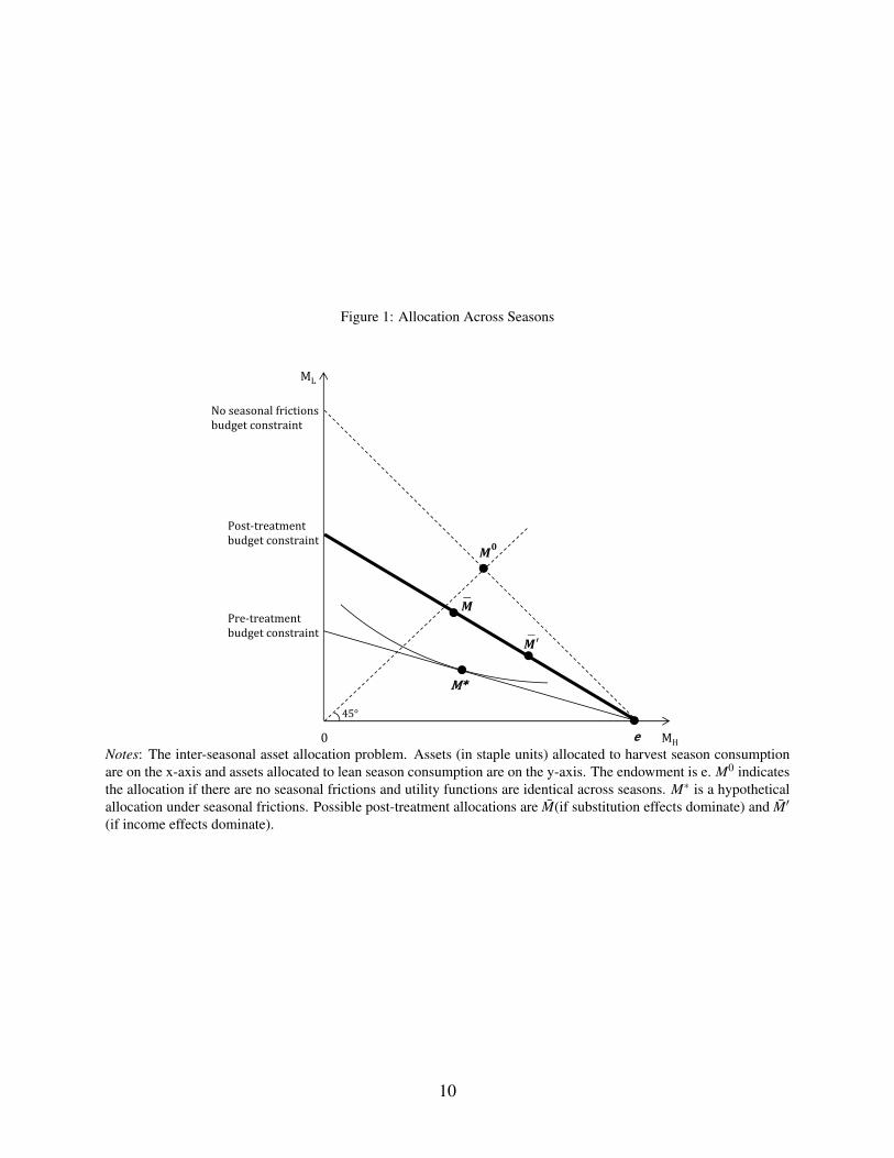
Figure 1: Allocation Across Seasons

MH

ML

e0

45°

Pre‐treatmentbudgetconstraint

Post‐treatmentbudgetconstraint

Noseasonalfrictionsbudgetconstraint

M*

′

Figure 1: The inter‐seasonal asset allocation problem. Assets (in staple units) allocated to harvest season consumption are on the x‐axis and assets allocated to lean season consumption are on the y‐axis. The endowment is e. M0 indicates the allocation if there are no seasonal frictions and utility functions are identical across seasons. M* is a hypothetical allocation under seasonal frictions. Possible post‐treatment allocations are        (if substitution effects dominate) and         (if income effects dominate).′

Notes: The inter-seasonal asset allocation problem. Assets (in staple units) allocated to harvest season consumptionare on the x-axis and assets allocated to lean season consumption are on the y-axis. The endowment is e. M0 indicatesthe allocation if there are no seasonal frictions and utility functions are identical across seasons. M∗ is a hypotheticalallocation under seasonal frictions. Possible post-treatment allocations are M̄(if substitution effects dominate) and M̄′

(if income effects dominate).

10

Second, the new levels of MH and ML result in new allocations of food and non-food consump-tion within each season. How a change in Mt is allocated across mt and ct depends on rates ofchange of marginal utilities (u′m,t , u′c,t). Under homothetic utility, we expect a rise in both formsof consumption. On the other hand, if individuals are close to food satiation, most changes willbe captured by non-food consumption. A quasilinear utility function helps demonstrate this point:the first tranches of income are allocated to food, but additional income gains are directed towardsnon-food consumption. The predictions are summarized in the table below, where the asteriskserves as a reminder that there could be no effect for staple consumption under quasi-linear utility.

Storage/Credit Harvest LeanIf income effect dominates:Non-food consumption (c) ↑ ↑Staple consumption (m)∗ ↑ ↑

If substitution effect dominates:Non-food consumption (c) ↓ ↑Staple consumption (m)∗ ↓ ↑

4. Program Design

Given global concerns about food security and the high costs of food programs, we were ap-proached by the World Bank to design and evaluate new solutions in West Timor, a setting withhistorical food insecurity and predictable seasonal patterns. While both programs have features thatare tailored to West Timor, they share similarities with other food programs. See Gelay (2008),Lines (2011) and Zeller (2001) for examples of food storage programs and Khandker and Mahmud(2012) and Mohan et al. (2007) for examples of credit programs for consumption purposes.

The implementation and evaluation of the programs were funded by the Japanese Social Devel-opment Fund. The treatments were implemented in September 2008 and lasted 3 years. The pro-grams were implemented by two local NGOs, Yayasan Alfa Omega (YAO) and Yayasan TanaobaLais Manekat (TLM), each of which operated independently in two districts. YAO operated inthe districts of Kupang and Timor Tengah Utara (TTU) while TLM operated in districts of TimorTengah Selatan (TTS) and Belu. Maize is the primary crop on the island, but some regions alsoplant rice, depending on the growing conditions. In TLM districts, a larger proportion of farmersexclusively grow maize than in YAO districts.18

Both NGOs were selected because they had experience implementing cash-based savings andmicrocredit programs in West Timor. Participants were informed that the food storage and foodcredit programs were part of a three-year pilot, sponsored by the World Bank. Both were intro-duced as new programs, with no ties to other programs sponsored by the NGOs. All facilitators onthe field were newly hired and trained.

The project covered 24 rural villages in each of the four districts, or kabupatens, in West Timor.These villages were selected by the NGOs, who were instructed to choose villages that were farenough from each other to avoid contamination effects.

18In our data, 96% of households report some maize production during our sample period. During the first harvest,62% of farm households in TLM districts reported producing maize only and 10% produced both maize and rice. Bycontrast, 34% of farm households in YAO districts reported producing maize only and 43% reported producing bothmaize and rice.

11

Treatment assignment was conducted by us and stratified by district. Within each district,six villages were randomly assigned to the control group (no treatment), twelve to the storagetreatment, and six to the credit treatment. To be eligible for storage or credit programs, the NGOsrequired participants to be married (or once-married) female farmers.

While the impacts on consumption, for both storage and credit, can be analyzed within theframework of income and substitution effects provided in Section 3, each is distinct in its im-plementation. Below, we describe in detail the implementation of each program and associatedtheories of change.

4.1. Storage4.1.1. Design

The storage treatment was designed to subsidize lean season consumption by raising the reten-tion rate which, as described in Section 2, is constrained by physical depreciation, social pressures,and price variation. The program provided new storage equipment for free. Participants wereoffered a choice of high capacity drums (180 kg), lower capacity jerrycans (40 kg), and sacks.

In total, there were 2,433 members under YAO and 2,529 members under TLM. Groups of upto 108 women per village were formed through public announcements in the lean season. Whiletraining was provided at the group level, grain was stored privately. Participants were trained indrying methods and provided with warnings about aflatoxins which can destroy large quantities ifthe grain is exposed to moisture. Compared to traditional methods of hanging smoked maize, thesetechnologies discouraged frequent withdrawals (which would expose the dried maize to moistureand air). Drums were the most popular method of storage, and more than 80% of stored stapleswere maize.19

For the first year, we imported storage products from another island. Materials arrived too lateto be used in the harvest season of that year. This meant that storage treatments in most areasstarted in the harvest season of the second year. For the second year, our agricultural specialistsmanaged to locally source sufficiently secure storage materials.

Given these delays and the finiteness of our survey timeline, we were left with a limited windowof opportunity to evaluate the effects of storage. This is a potential concern since the potentialbenefits of storage are realized only after adequate harvests. In the short run, harvest failures leavehouseholds with little to store.

19We had initially designed two storage treatments: a "pure storage" treatment in which participants were free towithdraw at any time, and a "commitment storage" treatment in which they agreed to a restriction on withdrawalsuntil a self-specified date. Each was assigned to a quarter of the villages. Under commitment storage, individualswere required to sign a contract under which they agreed to a restriction on withdrawals until a self-specified date.The contract allowed for early withdrawals only in the case of explicitly defined and verifiable emergencies. Storageequipment was then sealed. The implementing NGOs were tasked with carrying out random audits to check the seal.If the seal was broken before the contracted date, and if the individual did not have a verifiable emergency, she wouldbe denied future access to the program.

In practice, however, the implementing NGOs did not adhere to this distinction. Under even the pure storagetreatment, participants were required to maintain written records specifying anticipated withdrawal dates. While thesewere not contractually binding, they served to discourage them from making intermediate withdrawals. For thesereasons, we do not distinguish between the pure storage and contract storage treatments in our analysis. We repeatedthe empirical analysis treating pure and contract villages separately. There were no differences between the twotreatment groups.

12

On the other hand, a particular advantage of the storage program is that it might reduce house-hold vulnerability to self-control problems and social pressures (Ashraf et al., 2006). This is be-cause the nature of the technology both discourages frequent withdrawals and reduces visibility ofstored assets.

4.1.2. Predicted First-Stage Effects for StorageSection 3 maps out the overall change in consumption that is predicted through participation

in either program. Consumption must be preceded by intermediate choices, which are affecteddifferentially by storage and credit. Here, we extend our model to predict how each programaffects the following intermediate outcomes which are potentially observable: stored staple stocksafter harvest and at the start of the lean season, and staple sales. We first conduct this exercise forstorage.

Figure 2 serves as a guide to farmers’ decisions that ultimately result in consumption. Thevariables that we analyze in our data analysis are indicated in capital letters. Consider choices inthe absence of storage and credit programs. The top panel of the figure shows decisions madein the harvest season. Harvested staple must be allocated across harvest and lean seasons. Theamount allocated to the harvest season can be consumed in kind (mH) or as non-food (cH) forwhich staples are sold. The portion of harvested staple that is not immediately consumed mustbe transferred to the lean season. As described in Section 3, this can be done using any of threetechnologies (in-kind savings, cash savings, in-kind credit). In the lean season, the farmer observesher assets and converts them into consumption.

Now, consider the impact of the storage program, which raises the staple retention rate to someγ̄ . Assume households were initially saving in kind or in cash at some η < γ̄ (since credit usewas rare). The resulting changes in behavior depend on whether income or substitution effectsdominate, and whether households were originally saving in kind or in cash. The following tablesummarizes the predicted changes in behavior.

Storage Harvest LeanIf income effect dominates:Staple sales ↑ (in-kind savers), ↓ (cash savers) ↑ (to fund non-food consumption)Staple stock ↓ (in-kind savers), ↑ (cash savers) ↑ (higher retention rate)If substitution effect dominates:Staple sales ↓ (more saved in kind) ↑ (to fund non-food consumption)Staple stock ↑ (less consumed) ↑ (more stored, higher retention rate)

The impacts on consumption are as described in Section 3.2. The table above allows us tomake some additional observations relevant to the data analysis. First, lean season predictions arestraightforward. Stocks should unambiguously expand, regardless of the initial technology. Leanseason staple sales should also rise to fund the increase in non-food consumption that results froman expanded lean season budget.

Second, harvest season predictions are ambiguous if income effects dominate–in this case,harvest season consumption increases. The changes on intermediate outcomes depend on the initialtechnology used. Stored stocks could fall or rise: those who were initially saving in kind will storeless to fund greater consumption in the harvest season, but those who were initially saving in cash

13

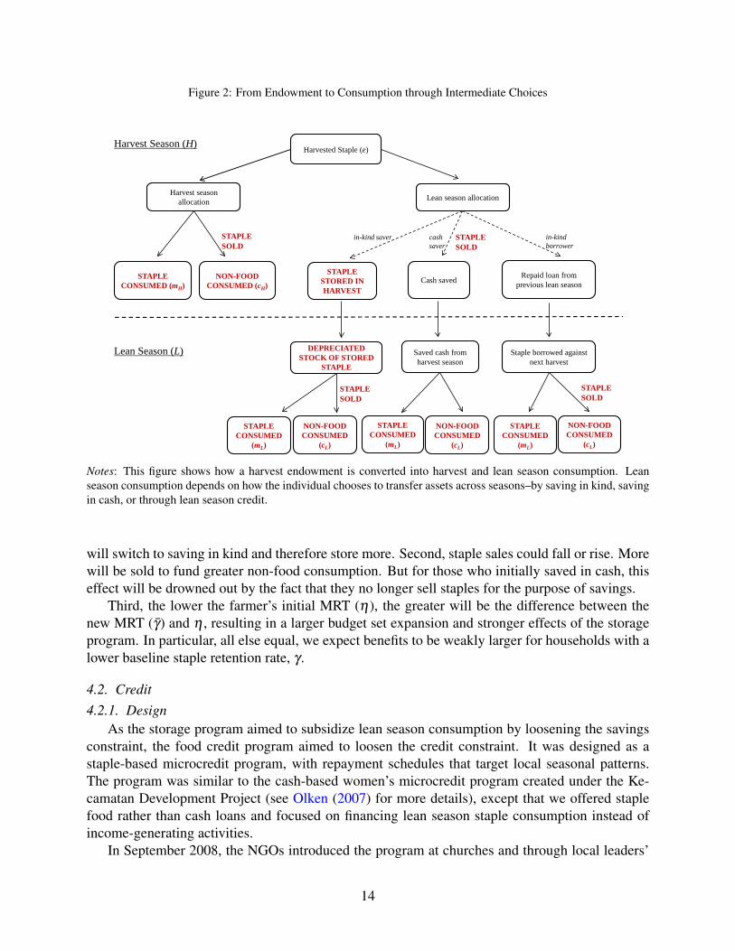
Figure 2: From Endowment to Consumption through Intermediate Choices

Harvested Staple (e)

Harvest season allocation Lean season allocation

STAPLE STORED IN HARVEST

Cash saved Repaid loan from previous lean season

DEPRECIATED STOCK OF STORED

STAPLE

Saved cash from harvest season

Staple borrowed against next harvest

STAPLE CONSUMED (mH)

NON-FOOD CONSUMED (cH)

in-kind saver cash saver

in-kind borrower

STAPLE SOLD

Harvest Season (H)

Lean Season (L)

STAPLE SOLD

STAPLE SOLD

STAPLE SOLD

STAPLE CONSUMED

(mL)

NON-FOOD CONSUMED

(cL)

STAPLE CONSUMED

(mL)

NON-FOOD CONSUMED

(cL)

STAPLE CONSUMED

(mL)

NON-FOOD CONSUMED

(cL)

Notes: This figure shows how a harvest endowment is converted into harvest and lean season consumption. Leanseason consumption depends on how the individual chooses to transfer assets across seasons–by saving in kind, savingin cash, or through lean season credit.

will switch to saving in kind and therefore store more. Second, staple sales could fall or rise. Morewill be sold to fund greater non-food consumption. But for those who initially saved in cash, thiseffect will be drowned out by the fact that they no longer sell staples for the purpose of savings.

Third, the lower the farmer’s initial MRT (η), the greater will be the difference between thenew MRT (γ̄) and η , resulting in a larger budget set expansion and stronger effects of the storageprogram. In particular, all else equal, we expect benefits to be weakly larger for households with alower baseline staple retention rate, γ .

4.2. Credit4.2.1. Design

As the storage program aimed to subsidize lean season consumption by loosening the savingsconstraint, the food credit program aimed to loosen the credit constraint. It was designed as astaple-based microcredit program, with repayment schedules that target local seasonal patterns.The program was similar to the cash-based women’s microcredit program created under the Ke-camatan Development Project (see Olken (2007) for more details), except that we offered staplefood rather than cash loans and focused on financing lean season staple consumption instead ofincome-generating activities.

In September 2008, the NGOs introduced the program at churches and through local leaders’

14

networks. Credit groups of up to 108 eligible women were formed in each treated village. Groupsthen elected their internal leaders and administrators. In total, there were 1229 and 1374 creditparticipants in YAO and TLM villages, respectively.

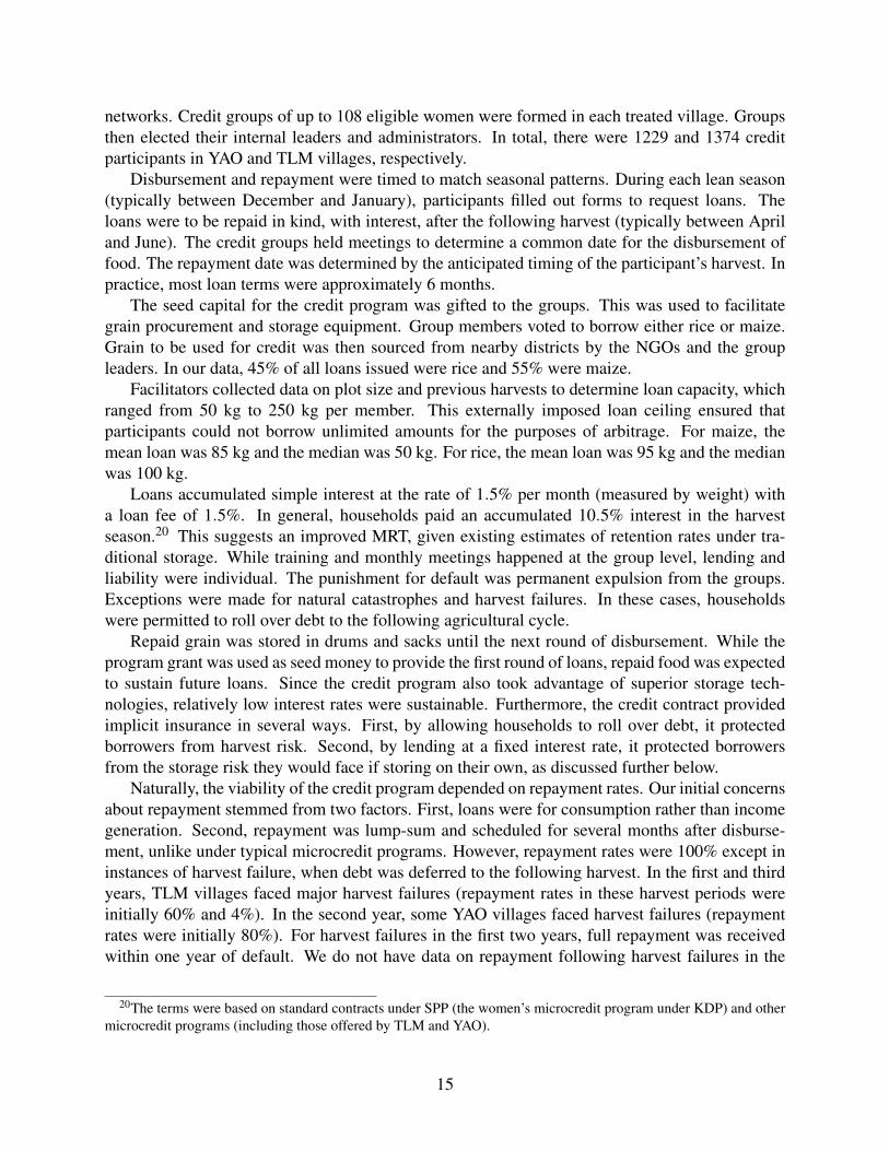
Disbursement and repayment were timed to match seasonal patterns. During each lean season(typically between December and January), participants filled out forms to request loans. Theloans were to be repaid in kind, with interest, after the following harvest (typically between Apriland June). The credit groups held meetings to determine a common date for the disbursement offood. The repayment date was determined by the anticipated timing of the participant’s harvest. Inpractice, most loan terms were approximately 6 months.

The seed capital for the credit program was gifted to the groups. This was used to facilitategrain procurement and storage equipment. Group members voted to borrow either rice or maize.Grain to be used for credit was then sourced from nearby districts by the NGOs and the groupleaders. In our data, 45% of all loans issued were rice and 55% were maize.

Facilitators collected data on plot size and previous harvests to determine loan capacity, whichranged from 50 kg to 250 kg per member. This externally imposed loan ceiling ensured thatparticipants could not borrow unlimited amounts for the purposes of arbitrage. For maize, themean loan was 85 kg and the median was 50 kg. For rice, the mean loan was 95 kg and the medianwas 100 kg.

Loans accumulated simple interest at the rate of 1.5% per month (measured by weight) witha loan fee of 1.5%. In general, households paid an accumulated 10.5% interest in the harvestseason.20 This suggests an improved MRT, given existing estimates of retention rates under tra-ditional storage. While training and monthly meetings happened at the group level, lending andliability were individual. The punishment for default was permanent expulsion from the groups.Exceptions were made for natural catastrophes and harvest failures. In these cases, householdswere permitted to roll over debt to the following agricultural cycle.

Repaid grain was stored in drums and sacks until the next round of disbursement. While theprogram grant was used as seed money to provide the first round of loans, repaid food was expectedto sustain future loans. Since the credit program also took advantage of superior storage tech-nologies, relatively low interest rates were sustainable. Furthermore, the credit contract providedimplicit insurance in several ways. First, by allowing households to roll over debt, it protectedborrowers from harvest risk. Second, by lending at a fixed interest rate, it protected borrowersfrom the storage risk they would face if storing on their own, as discussed further below.

Naturally, the viability of the credit program depended on repayment rates. Our initial concernsabout repayment stemmed from two factors. First, loans were for consumption rather than incomegeneration. Second, repayment was lump-sum and scheduled for several months after disburse-ment, unlike under typical microcredit programs. However, repayment rates were 100% except ininstances of harvest failure, when debt was deferred to the following harvest. In the first and thirdyears, TLM villages faced major harvest failures (repayment rates in these harvest periods wereinitially 60% and 4%). In the second year, some YAO villages faced harvest failures (repaymentrates were initially 80%). For harvest failures in the first two years, full repayment was receivedwithin one year of default. We do not have data on repayment following harvest failures in the

20The terms were based on standard contracts under SPP (the women’s microcredit program under KDP) and othermicrocredit programs (including those offered by TLM and YAO).

15

third year as the formal program had ended by that time. The high repayment rates suggest thatsuch a program can be self-sustaining.

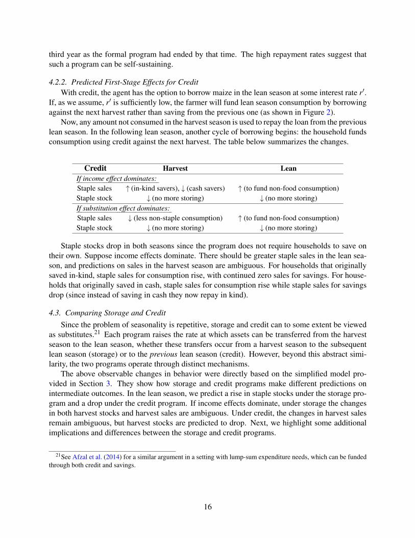
4.2.2. Predicted First-Stage Effects for CreditWith credit, the agent has the option to borrow maize in the lean season at some interest rate r′.

If, as we assume, r′ is sufficiently low, the farmer will fund lean season consumption by borrowingagainst the next harvest rather than saving from the previous one (as shown in Figure 2).

Now, any amount not consumed in the harvest season is used to repay the loan from the previouslean season. In the following lean season, another cycle of borrowing begins: the household fundsconsumption using credit against the next harvest. The table below summarizes the changes.

Credit Harvest LeanIf income effect dominates:Staple sales ↑ (in-kind savers), ↓ (cash savers) ↑ (to fund non-food consumption)Staple stock ↓ (no more storing) ↓ (no more storing)If substitution effect dominates:Staple sales ↓ (less non-staple consumption) ↑ (to fund non-food consumption)Staple stock ↓ (no more storing) ↓ (no more storing)

Staple stocks drop in both seasons since the program does not require households to save ontheir own. Suppose income effects dominate. There should be greater staple sales in the lean sea-son, and predictions on sales in the harvest season are ambiguous. For households that originallysaved in-kind, staple sales for consumption rise, with continued zero sales for savings. For house-holds that originally saved in cash, staple sales for consumption rise while staple sales for savingsdrop (since instead of saving in cash they now repay in kind).

4.3. Comparing Storage and CreditSince the problem of seasonality is repetitive, storage and credit can to some extent be viewed

as substitutes.21 Each program raises the rate at which assets can be transferred from the harvestseason to the lean season, whether these transfers occur from a harvest season to the subsequentlean season (storage) or to the previous lean season (credit). However, beyond this abstract simi-larity, the two programs operate through distinct mechanisms.

The above observable changes in behavior were directly based on the simplified model pro-vided in Section 3. They show how storage and credit programs make different predictions onintermediate outcomes. In the lean season, we predict a rise in staple stocks under the storage pro-gram and a drop under the credit program. If income effects dominate, under storage the changesin both harvest stocks and harvest sales are ambiguous. Under credit, the changes in harvest salesremain ambiguous, but harvest stocks are predicted to drop. Next, we highlight some additionalimplications and differences between the storage and credit programs.

21See Afzal et al. (2014) for a similar argument in a setting with lump-sum expenditure needs, which can be fundedthrough both credit and savings.

16

4.3.1. RiskRisk can matter differently for credit and storage. We argue that credit is better than storage at

dampening the fluctuations associated with risky outcomes. This happens through the programs’interaction with both harvest risk and storage risk.

First, the benefits of storage depend on the realized harvest. Under harvest failure, if there isnothing to store, there is nothing to be gained from improved storage. Credit, on the other hand,provides implicit insurance through limited liability. Furthermore, the group lending aspect ofcredit encourages risk sharing across members.

Second, under storage, households face a risk even conditional on harvest since the technolo-gies are not foolproof. For example, under certain conditions, stored maize could be damaged byaflatoxins. While the storage treatment is expected to raise the MRT, the actual rise in MRT is un-certain. This can limit the ability of households to precisely close seasonal gaps through storage.Under credit, this risk is absorbed by the program since the interest rate is fixed and is independentof storage risk. In effect, credit offers households a fixed MRT while storage does not. Therefore,when comparing consumption between any two consecutive harvest and lean seasons, we expectseasonal gaps to be lower under credit than under storage.

4.3.2. Social and Behavioral FactorsRecent literature in behavioral economics examines how savings and credit decisions are influ-

enced by one’s preferences (which might be time-inconsistent) and social relations (which resultin pressures to share, on the one hand, and provide discipline, on the other). These considerationsplay out differently in our storage and credit programs.

Storage provides informal commitment of two kinds. First, the technology and treatment de-sign discourage frequent withdrawals (Ashraf et al., 2006). Second, households have an oppor-tunity to reduce the visibility of their assets, and thus potentially protect themselves from socialtaxes (Baland et al., 2011).

Under credit, there is a concern about over-borrowing if individuals are time-inconsistent(Basu, 2014). Time-inconsistent preferences imply a desire to consume more in the present thanis optimal under some reasonable notions of long-run welfare. By offering consumption with de-layed payments, credit could help individuals indulge their taste for instant gratification, resultingin high debt burdens in the harvest season.

To some extent, this might be prevented by institutional limits to loan size. While a determina-tion of the optimal loan size is beyond the scope of this paper, we provide some evidence from theannual Indonesian Susenas household survey to suggest that our program loan limits leave roomfor over-borrowing. We find that the maximum loan of 250 kg provides more than 4 months of theaverage staple consumption for farm households in West Timor.22 It is therefore possible that theprogram would enable households with self-control problems to consume more in the lean seasonthan would be in their long-run interest.

22According to the Susenas household survey in 2008, the average farm household in West Timor consumes 1400calories per day from staples. To provide this, households require about 0.39 kg of rice or maize per day (1 kg ofrice and maize provide roughly 3600 calories). For a lean season period lasting 3 months (Dec-Feb), a household of 5would need 176 kg (0.39 kg *90 days*5 members). For 4 months (Nov-Feb), the equivalent number is 234 kg.

17

5. Data

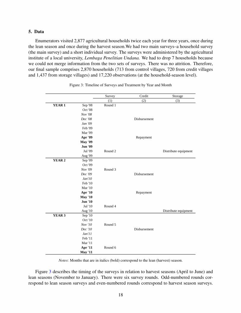
Enumerators visited 2,877 agricultural households twice each year for three years, once duringthe lean season and once during the harvest season.We had two main surveys–a household survey(the main survey) and a short individual survey. The surveys were administered by the agriculturalinstitute of a local university, Lembaga Penelitian Undana. We had to drop 7 households becausewe could not merge information from the two sets of surveys. There was no attrition. Therefore,our final sample comprises 2,870 households (713 from control villages, 720 from credit villagesand 1,437 from storage villages) and 17,220 observations (at the household-season level).

Figure 3: Timeline of Surveys and Treatment by Year and Month

Survey Credit Storage(1) (2) (3)

YEAR 1 Sep '08 Round 1Oct '08

Nov '08Dec '08 DisbursementJan '09Feb '09Mar '09Apr '09 RepaymentMay '09Jun '09

Jul '09 Round 2 Distribute equipmentAug '09

YEAR 2 Sep '09Oct '09

Nov '09 Round 3Dec '09 DisbursementJan'10Feb '10Mar '10Apr '10 RepaymentMay '10Jun '10

Jul '10 Round 4Aug '10 Distribute equipment

YEAR 3 Sep '10Oct '10

Nov '10 Round 5Dec '10 DisbursementJan'11Feb '11Mar '11Apr '11 Round 6May '11

Note: Months that are in italics (bold) correspond to the lean (harvest) season.Notes: Months that are in italics (bold) correspond to the lean (harvest) season.

Figure 3 describes the timing of the surveys in relation to harvest seasons (April to June) andlean seasons (November to January). There were six survey rounds. Odd-numbered rounds cor-respond to lean season surveys and even-numbered rounds correspond to harvest season surveys.

18

Column 1 shows that the first round was conducted between September and November 2008, justbefore the start of the lean season. Because many of the villages were extremely remote, eachsurvey round took two to three months to complete. Due to budget delays, the first two harvestseason surveys (rounds 2 and 4) were delayed by three months and began in July.

The following columns in Figure 3 show how the timing of the surveys coincided with the treat-ments. For credit, food disbursements occurred between the months of December and January (thepeak of the lean season) and repayments were around harvest months (April to June). Comparingcolumns 1 and 2, we can see that credit has five rounds of post-treatment surveys (rounds 2 to 6)and one pre-treatment round that was conducted in the lean season. We do not have a pre-treatmentharvest season survey for credit.

For storage, the final column shows that equipment only arrived between July and August of2009 (coinciding with round 2, in column 1). Since this was already several months after thefirst harvest, little was stored until the subsequent harvest season (round 4). Therefore, we definerounds 4 to 6 as post treatment rounds for storage. We have one pre-treatment harvest survey andtwo pre-treatment lean surveys.

Key outcomesWe constructed the following measures to test whether our treatments improved well-being

by raising consumption and health or reducing seasonal fluctuations. We first construct measuresto test for consumption effects discussed in Section 3.2, including log(Staple consumed, kCal),23

log(Non-food expenditure), log(Reported income) and an indicator that is one if the householdreported lacking food in the previous month. All continuous consumption measures are scaled toper capita per month units. Reported income is the amount households report as their income (fromharvest sales, wages, remittances and gifts). We explain how these variables are constructed andrelated data issues (such as outliers and missing values) in Table A1 in the appendix.

We also included self-reported measures related to health. We have three variables–an indicatorvariable of whether the household was unable to afford health expenditures in the past month, thenumber of household members who reported any sickness in the past three months, and the totalnumber of sick days reported (totaled over all members who reported they were sick in the pastthree months). The last two health outcomes are scaled to per capita per month units.

Next, we measure seasonal fluctuations using the absolute difference between consumption inthe harvest and lean seasons within each agricultural cycle.24 Reductions in seasonal gaps can beinterpreted as a welfare improvement, under the assumption of identical, separable, and concaveutility functions for both seasons. We provide more details in the appendix where we also reportresults using other measures of consumption variability.

To address concerns associated with having many outcomes, we follow Kling et al. (2007) anduse mean effects analysis. We discuss mean effects analysis in the appendix.

One limitation of our data is that our food intake information is incomplete. We have consump-tion measures for primary staples and other major food items (cassava, fruits and beans). Rice and

23Staple consumption is calculated as rice consumed plus maize consumed (both in calories), as these are the twomain staples.

24For example, the seasonal gap in log(Staple consumed) is measured as the absolute difference between rounds 2and 3 and the absolute difference between rounds 4 and 5. For seasonal differences, we use differences in the monthlynon-food expenditure items only. See Table A1 in the appendix.

19

maize represent more than 60% of the average per capita per day calories for farmers in rural WestTimor, based on our calculations using the 2008 annual Susenas household survey. Other studieshave also found that about 60% to 70% of calories in the typical poor person’s diet comes from theprimary staple in the region (see, for example, Jensen and Miller (2011)). For budgetary reasons,we did not collect data on other foods such as meat and seafood. As a result, we are unable to builda truly comprehensive measure of food consumption. If households substituted towards consumingnon-staples not measured by us, our analysis will miss this margin of adjustment.

Another limitation lies in the measurement of staple inventory. Since the traditional storagemethod involves hanging smoked maize in the attic, it was hard to measure the weight of themaize inventory, especially in the control villages. Also, the timing of measurement was crucial.As discussed in Section 4, we would ideally measure whether the storage treatment expanded thestock of inventory at the beginning of the lean season, before any sales or consumption of thestaple stock. In practice, we often surveyed the villages closer to the peak of the lean seasons (lateNovember to January), when most households would have already sold or consumed some of theirstaple stock.

Balance checksTable 2 reports results from tests of whether treatment and control villages are balanced, using

the first survey round. Column 1 of Table 2 reports the means of the control group in the baseline(round 1, lean season). The average amount of calories consumed per capita per month is 40.88kCals. The average absolute difference in staples consumed across seasons is 24.52 kCals. Onaverage, 6.7% of households report some savings in a bank, 11.8% of households report havingsome debt, the maize inventory is 29% of the maize produced and the rice inventory is 24% of therice produced.

Columns 3 to 5 report results from OLS regressions comparing storage to control villages,controlling for district fixed effects and clustering standard errors at the village level. We reportp-values for tests of the coefficient on the treatment indicator being zero. Columns 6 to 8 reportresults for credit versus control villages. The full estimation samples include 2,150 households forstorage and 1,433 households for credit. The outcomes are organized into five panels: Panel A in-cludes consumption and income, Panel B includes health outcomes, Panel C examines agriculturalproduction and storage behavior and Panel D reports baseline household characteristics and PanelE reports baseline seasonal differences.

For storage, one outcome out of 23 tests has a p-value below 5%. In Panel D, Number ofmotorcycles owned has a mean difference of 0.051 and a p-value of 0.8% (compared to the controlgroup mean of 0.067). However, a difference of 0.051 motorcycles seems small and economicallyinsubstantial. For credit, Table 2 shows no p-values below 5%.

6. Estimation

We use an Intent-to-Treat (ITT) specification that compares treatment and control villages:

yivd = α +βT REAT vd +θd + εivd (6)

where yivd is the outcome for household i, in village v in district d, T REATvd is the treatmentassignment indicator and θd represents district fixed effects (treatment assignment was stratifiedby districts). We estimate the regressions separately for credit and for storage and pool all post

20

treatment survey rounds. Standard errors are clustered at the village level. The take-up rate forcredit was 40% and the take-up rate for storage was 42%.

The key parameter of interest, β , represents the average treatment effect of being in a villagethat was assigned either credit or storage (compared to no treatment). We expect an improvementin well-being to be associated with increases in consumption levels and improvements in healthand decreases in seasonal differences. As discussed in Section 3.2, for consumption in the har-vest season, we expect β > 0 if the income effect dominates and β < 0 if the substitution effectdominates. For consumption in the lean season, we expect β > 0.

Unfortunately, due to a mis-communication, TLM assigned the wrong treatment for six vil-lages.25 To address this, we report our main results using only the initial intended assignment. Webelieve the non-compliance is orthogonal to unobserved village characteristics. The assignmentwas performed by the authors who were based in the United States at the time of assignment. Thetreatment assignment was sent via email but one NGO mistakenly used the treatment assignmentfrom an older email.

We also report heterogeneous treatment effect estimates by NGO districts. Since assignmentwas stratified by districts ex ante and both NGOs were operating independently, these results re-main internally valid. These regional patterns are worth examining for the following reasons. First,harvest risks are related to regional rainfall patterns, resulting in widespread harvest failures thatcan encompass entire districts. In the first two harvests, close to a fifth of maize farmers reportedzero maize production.26 In the final harvest, a prolonged rainy season linked to La Nina in 2010-2011 resulted in widespread harvest failures, with 70% of maize farmers reporting zero maizeproduction.

Second, TLM districts were more suitable for maize so that most farmers only planted maize(the riskier crop) while YAO districts had regions that were suitable for both maize and rice. There-fore, TLM districts experienced more harvest failures and the lack of crop diversification alsomeant that harvest failures were more costly. In the first harvest season, for example, maize farm-ers in TLM districts reported a 7 p.p. higher incidence of harvest failures, which is close to a thirdof the sample mean (22%). Relatedly, take-up rates tended to be lower in TLM than in YAO. Forstorage (credit), take-up was 35% (32%) for TLM compared to 49% (47%) for YAO. The greatersalience of harvest risks in TLM districts could explain the lower take-up. Farmers may not partic-ipate in credit because they are worried about their ability to repay, and farmers who experiencedharvest failures have nothing to store. This is less important for YAO districts because more farm-ers also produce and store rice. In the data collected by the NGOs, only 2% of households underTLM report storing any rice compared to 48% of households for YAO.

Finally, the mis-assignment problem was unique to TLM districts. We do not think the mis-assignment introduced systematic biases that can explain our results. In fact, we find strongereffects for YAO districts which suggests that our results are not driven by mis-assignment prob-lems. However, the mis-assignment problem remains significant for TLM districts (6 out of 48villages in TLM districts were mis-assigned) which could introduce more noise.

25Two villages assigned credit were implemented as storage villages, two villages assigned storage were imple-mented as credit and storage and credit were each implemented in a control village.

26Here, we define maize farmers as any farmer who produced some maize during our study period, which covers96% of households. Since maize is the primary staple and primary crop in West Timor, our assumption is that farmersplant maize every cycle, so that reports of zero maize production are most likely harvest failures.

21

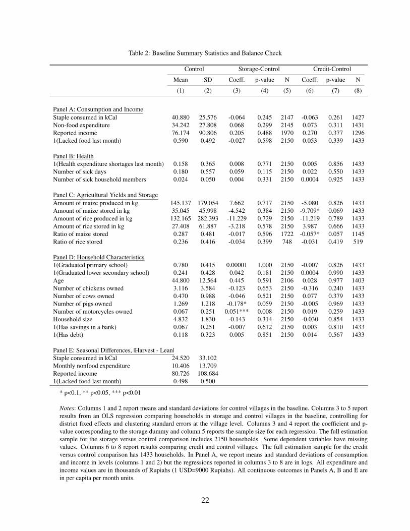
Table 2: Baseline Summary Statistics and Balance Check

Control Storage-Control Credit-Control

Mean SD Coeff. p-value N Coeff. p-value N

(1) (2) (3) (4) (5) (6) (7) (8)

Panel A: Consumption and IncomeStaple consumed in kCal 40.880 25.576 -0.064 0.245 2147 -0.063 0.261 1427Non-food expenditure 34.242 27.808 0.068 0.299 2145 0.073 0.311 1431Reported income 76.174 90.806 0.205 0.488 1970 0.270 0.377 12961(Lacked food last month) 0.590 0.492 -0.027 0.598 2150 0.053 0.339 1433

Panel B: Health1(Health expenditure shortages last month) 0.158 0.365 0.008 0.771 2150 0.005 0.856 1433Number of sick days 0.180 0.557 0.059 0.115 2150 0.022 0.550 1433Number of sick household members 0.024 0.050 0.004 0.331 2150 0.0004 0.925 1433

Panel C: Agricultural Yields and StorageAmount of maize produced in kg 145.137 179.054 7.662 0.717 2150 -5.080 0.826 1433Amount of maize stored in kg 35.045 45.998 -4.542 0.384 2150 -9.709* 0.069 1433Amount of rice produced in kg 132.165 282.393 -11.229 0.729 2150 -11.219 0.789 1433Amount of rice stored in kg 27.408 61.887 -3.218 0.578 2150 3.987 0.666 1433Ratio of maize stored 0.287 0.481 -0.017 0.596 1722 -0.057* 0.057 1145Ratio of rice stored 0.236 0.416 -0.034 0.399 748 -0.031 0.419 519

Panel D: Household Characteristics1(Graduated primary school) 0.780 0.415 0.00001 1.000 2150 -0.007 0.826 14331(Graduated lower secondary school) 0.241 0.428 0.042 0.181 2150 0.0004 0.990 1433Age 44.800 12.564 0.445 0.591 2106 0.028 0.977 1403Number of chickens owned 3.116 3.584 -0.123 0.653 2150 -0.316 0.240 1433Number of cows owned 0.470 0.988 -0.046 0.521 2150 0.077 0.379 1433Number of pigs owned 1.269 1.218 -0.178* 0.059 2150 -0.005 0.969 1433Number of motorcycles owned 0.067 0.251 0.051*** 0.008 2150 0.019 0.259 1433Household size 4.832 1.830 -0.143 0.314 2150 -0.030 0.854 14331(Has savings in a bank) 0.067 0.251 -0.007 0.612 2150 0.003 0.810 14331(Has debt) 0.118 0.323 0.005 0.851 2150 0.014 0.567 1433

Panel E: Seasonal Differences, |Harvest - Lean|Staple consumed in kCal 24.520 33.102Monthly nonfood expenditure 10.406 13.709Reported income 80.726 108.6841(Lacked food last month) 0.498 0.500

* p<0.1, ** p<0.05, *** p<0.01

Notes: Columns 1 and 2 report means and standard deviations for control villages in the baseline. Columns 3 to 5 reportresults from an OLS regression comparing households in storage and control villages in the baseline, controlling fordistrict fixed effects and clustering standard errors at the village level. Columns 3 and 4 report the coefficient and p-value corresponding to the storage dummy and column 5 reports the sample size for each regression. The full estimationsample for the storage versus control comparison includes 2150 households. Some dependent variables have missingvalues. Columns 6 to 8 report results comparing credit and control villages. The full estimation sample for the creditversus control comparison has 1433 households. In Panel A, we report means and standard deviations of consumptionand income in levels (columns 1 and 2) but the regressions reported in columns 3 to 8 are in logs. All expenditure andincome values are in thousands of Rupiahs (1 USD=9000 Rupiahs). All continuous outcomes in Panels A, B and E arein per capita per month units.

22

7. Results

We present the main results for the storage treatment in Section 7.1 and the results for the credittreatment in Section 7.2. We describe mechanisms in 7.3, provide cost benefit calculations in 7.4and discuss implications for future work in Section 7.5.

7.1. Main Results for StorageTable 3 reports results for consumption and reported income. Columns 1-3 report ITT estimates

for the storage treatment compared to the control group. Each pair of cells in this table reports theITT estimate of β in equation 6 and its standard error. We report results using all post treatmentseasons (column 1), lean seasons only (column 2) and harvest seasons only (column 3). Column4, labeled N(All), reports sample sizes for regressions in column 1. Panel A reports results for alldistricts. Panels B and C report results for YAO and TLM districts, respectively.

We find a statistically significant increase in the Consumption and Income Index by 0.097 (s.e.0.042) units for storage for all seasons (Panel A, column 1). The treatment effects are similar forboth lean (0.101, s.e. 0.054) and harvest seasons (0.095, s.e. 0.042). As discussed in Section 3.2,these increases, particularly in the harvest season, are consistent with dominant income effects dueto budget set expansions. The improvements are driven by a 13.4% (s.e. 7.7%) and a 14.2% (s.e.5.3%) increase in non-food expenditure in the lean and harvest seasons, respectively as well as a7.4 percentage point (s.e. 4.2. p.p.) decrease in the likelihood of food shortages in the lean season.The most responsive expenditure items seem to be discretionary personal consumption items. Bycomparison, Bryan et al. (2014) report ITT estimates implying that an US$8.50 migration subsidyin Bangladesh to encourage seasonal migration increased monthly per capita non-food consump-tion by 10.1% to 12.7%.

We estimate null effects on staple food consumption. The effects on consumption of staplecalories are 0.6% (s.e. 2.9%), with a 95 percent confidence interval of -5.1% to 6.3%. In caloriclevels scaled to per capita per day units, the 95 percent confidence intervals are -18 calories to 23calories, compared to the minimum daily recommendation of 2100 calories (commonly used toconstruct poverty estimates). Jensen and Miller (2011) study the impact of staple price subsidiesin China and find no evidence that subsidies improved nutrition, including calories consumed.They estimate 95 percent confidence intervals of a similar magnitude, -31 to 22 calories per personper day, for a ten percentage point increase in the subsidy of staple prices.27 Bryan et al. (2014)estimate calorie consumption effects of 4.5% to 5.1% and 95 percent confidence intervals of 82 to178 calories per capita per day.28

Given that the policy reduced the relative cost of lean season staple consumption, substitutioneffects should increase staple consumption in the lean season. However, we do not detect thisincrease. Moreover, transaction costs (which are likely to be significant for rural households)

27This was calculated using the -0.027 (s.e. 0.076) price elasticity estimate reported in Panel A in Table 4 for Jensenand Miller (2011). To calculate the impact on caloric levels, we use the average calories consumed per capita per dayfor the control group (1752 calories reported in Table 2). Therefore, the confidence intervals in calories per personper day (for a 10 percentage point increase in the price subsidy) are calculated as − 0.027

100 ∗10∗1752calories±1.96∗0.076100 ∗10∗1752calories. A ten percentage point price subsidy is roughly 0.11 RMB (US$0.01, 1RMB=$0.13), using

the average price in the two provinces in China, 1.1 RMB per 500 g of staple (see p1207 in Jensen and Miller (2011)).Each household received one month’s supply of vouchers for 750 g per person per day.

28Both Jensen and Miller (2011) and Bryan et al. (2014) ) include staple and non-staple calories.

23

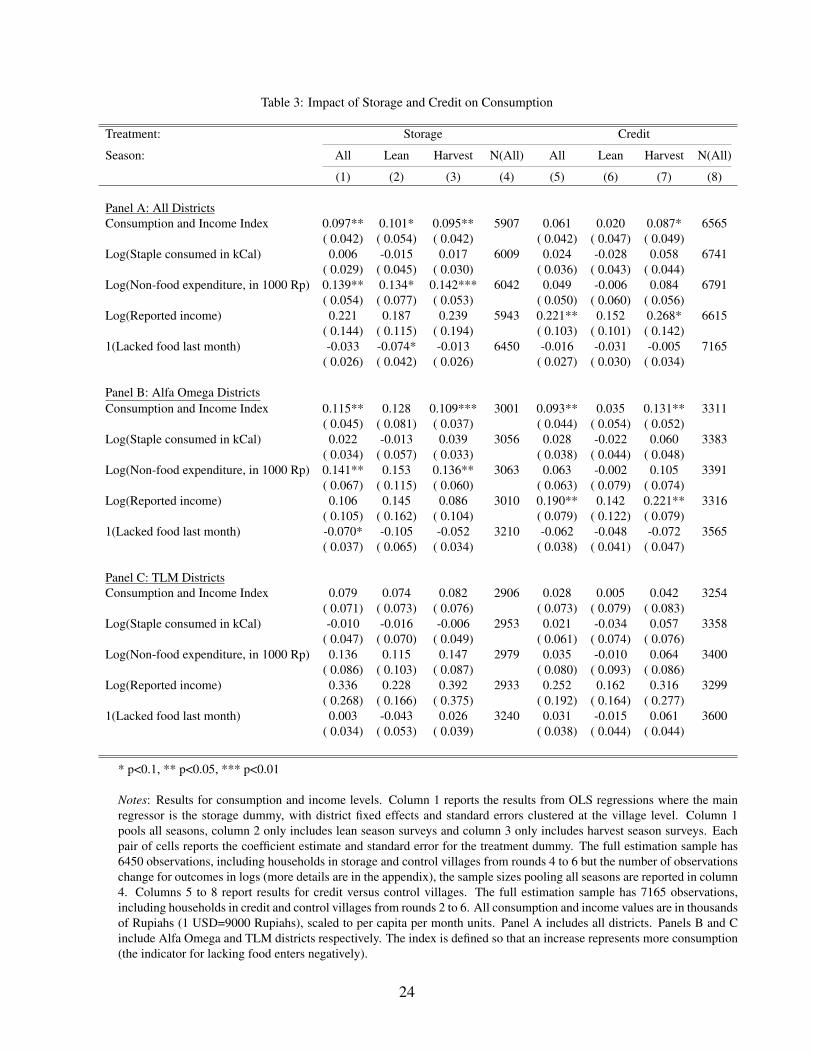
Table 3: Impact of Storage and Credit on Consumption

Treatment: Storage Credit

Season: All Lean Harvest N(All) All Lean Harvest N(All)

(1) (2) (3) (4) (5) (6) (7) (8)

Panel A: All DistrictsConsumption and Income Index 0.097** 0.101* 0.095** 5907 0.061 0.020 0.087* 6565

( 0.042) ( 0.054) ( 0.042) ( 0.042) ( 0.047) ( 0.049)Log(Staple consumed in kCal) 0.006 -0.015 0.017 6009 0.024 -0.028 0.058 6741

( 0.029) ( 0.045) ( 0.030) ( 0.036) ( 0.043) ( 0.044)Log(Non-food expenditure, in 1000 Rp) 0.139** 0.134* 0.142*** 6042 0.049 -0.006 0.084 6791

( 0.054) ( 0.077) ( 0.053) ( 0.050) ( 0.060) ( 0.056)Log(Reported income) 0.221 0.187 0.239 5943 0.221** 0.152 0.268* 6615

( 0.144) ( 0.115) ( 0.194) ( 0.103) ( 0.101) ( 0.142)1(Lacked food last month) -0.033 -0.074* -0.013 6450 -0.016 -0.031 -0.005 7165

( 0.026) ( 0.042) ( 0.026) ( 0.027) ( 0.030) ( 0.034)

Panel B: Alfa Omega DistrictsConsumption and Income Index 0.115** 0.128 0.109*** 3001 0.093** 0.035 0.131** 3311

( 0.045) ( 0.081) ( 0.037) ( 0.044) ( 0.054) ( 0.052)Log(Staple consumed in kCal) 0.022 -0.013 0.039 3056 0.028 -0.022 0.060 3383

( 0.034) ( 0.057) ( 0.033) ( 0.038) ( 0.044) ( 0.048)Log(Non-food expenditure, in 1000 Rp) 0.141** 0.153 0.136** 3063 0.063 -0.002 0.105 3391

( 0.067) ( 0.115) ( 0.060) ( 0.063) ( 0.079) ( 0.074)Log(Reported income) 0.106 0.145 0.086 3010 0.190** 0.142 0.221** 3316

( 0.105) ( 0.162) ( 0.104) ( 0.079) ( 0.122) ( 0.079)1(Lacked food last month) -0.070* -0.105 -0.052 3210 -0.062 -0.048 -0.072 3565

( 0.037) ( 0.065) ( 0.034) ( 0.038) ( 0.041) ( 0.047)

Panel C: TLM DistrictsConsumption and Income Index 0.079 0.074 0.082 2906 0.028 0.005 0.042 3254

( 0.071) ( 0.073) ( 0.076) ( 0.073) ( 0.079) ( 0.083)Log(Staple consumed in kCal) -0.010 -0.016 -0.006 2953 0.021 -0.034 0.057 3358

( 0.047) ( 0.070) ( 0.049) ( 0.061) ( 0.074) ( 0.076)Log(Non-food expenditure, in 1000 Rp) 0.136 0.115 0.147 2979 0.035 -0.010 0.064 3400

( 0.086) ( 0.103) ( 0.087) ( 0.080) ( 0.093) ( 0.086)Log(Reported income) 0.336 0.228 0.392 2933 0.252 0.162 0.316 3299

( 0.268) ( 0.166) ( 0.375) ( 0.192) ( 0.164) ( 0.277)1(Lacked food last month) 0.003 -0.043 0.026 3240 0.031 -0.015 0.061 3600

( 0.034) ( 0.053) ( 0.039) ( 0.038) ( 0.044) ( 0.044)

* p<0.1, ** p<0.05, *** p<0.01

Notes: Results for consumption and income levels. Column 1 reports the results from OLS regressions where the mainregressor is the storage dummy, with district fixed effects and standard errors clustered at the village level. Column 1pools all seasons, column 2 only includes lean season surveys and column 3 only includes harvest season surveys. Eachpair of cells reports the coefficient estimate and standard error for the treatment dummy. The full estimation sample has6450 observations, including households in storage and control villages from rounds 4 to 6 but the number of observationschange for outcomes in logs (more details are in the appendix), the sample sizes pooling all seasons are reported in column4. Columns 5 to 8 report results for credit versus control villages. The full estimation sample has 7165 observations,including households in credit and control villages from rounds 2 to 6. All consumption and income values are in thousandsof Rupiahs (1 USD=9000 Rupiahs), scaled to per capita per month units. Panel A includes all districts. Panels B and Cinclude Alfa Omega and TLM districts respectively. The index is defined so that an increase represents more consumption(the indicator for lacking food enters negatively).

24

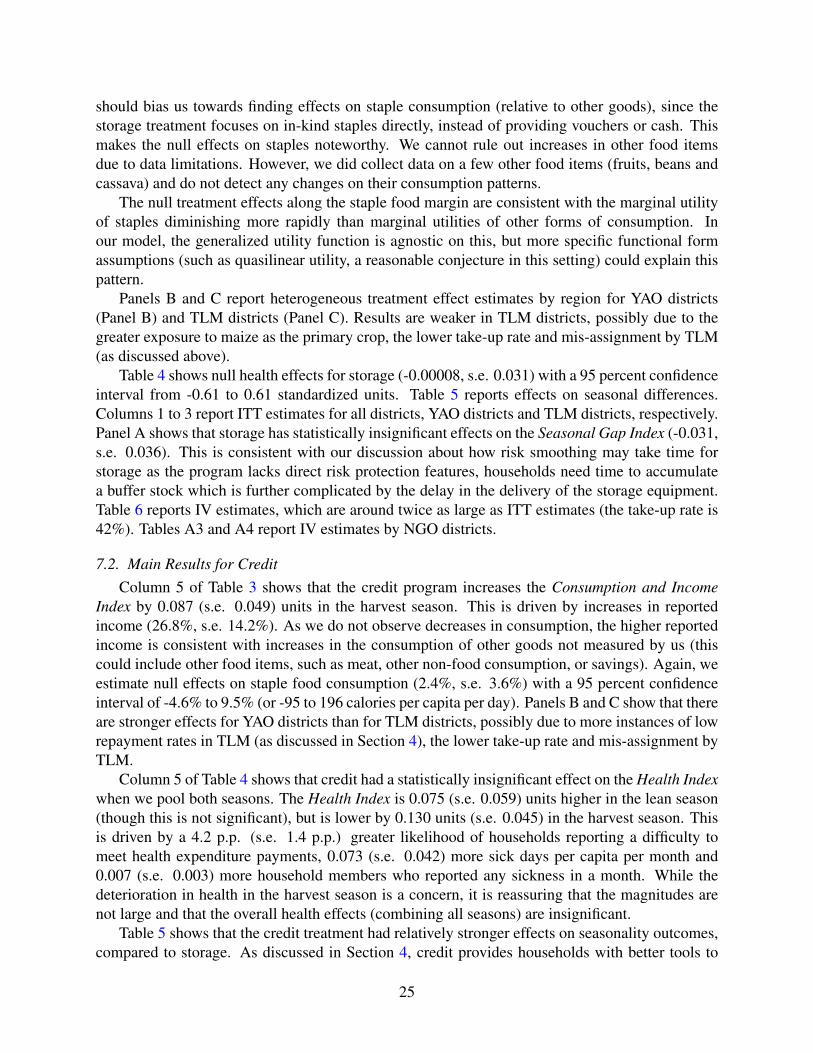
should bias us towards finding effects on staple consumption (relative to other goods), since thestorage treatment focuses on in-kind staples directly, instead of providing vouchers or cash. Thismakes the null effects on staples noteworthy. We cannot rule out increases in other food itemsdue to data limitations. However, we did collect data on a few other food items (fruits, beans andcassava) and do not detect any changes on their consumption patterns.

The null treatment effects along the staple food margin are consistent with the marginal utilityof staples diminishing more rapidly than marginal utilities of other forms of consumption. Inour model, the generalized utility function is agnostic on this, but more specific functional formassumptions (such as quasilinear utility, a reasonable conjecture in this setting) could explain thispattern.

Panels B and C report heterogeneous treatment effect estimates by region for YAO districts(Panel B) and TLM districts (Panel C). Results are weaker in TLM districts, possibly due to thegreater exposure to maize as the primary crop, the lower take-up rate and mis-assignment by TLM(as discussed above).

Table 4 shows null health effects for storage (-0.00008, s.e. 0.031) with a 95 percent confidenceinterval from -0.61 to 0.61 standardized units. Table 5 reports effects on seasonal differences.Columns 1 to 3 report ITT estimates for all districts, YAO districts and TLM districts, respectively.Panel A shows that storage has statistically insignificant effects on the Seasonal Gap Index (-0.031,s.e. 0.036). This is consistent with our discussion about how risk smoothing may take time forstorage as the program lacks direct risk protection features, households need time to accumulatea buffer stock which is further complicated by the delay in the delivery of the storage equipment.Table 6 reports IV estimates, which are around twice as large as ITT estimates (the take-up rate is42%). Tables A3 and A4 report IV estimates by NGO districts.

7.2. Main Results for CreditColumn 5 of Table 3 shows that the credit program increases the Consumption and Income

Index by 0.087 (s.e. 0.049) units in the harvest season. This is driven by increases in reportedincome (26.8%, s.e. 14.2%). As we do not observe decreases in consumption, the higher reportedincome is consistent with increases in the consumption of other goods not measured by us (thiscould include other food items, such as meat, other non-food consumption, or savings). Again, weestimate null effects on staple food consumption (2.4%, s.e. 3.6%) with a 95 percent confidenceinterval of -4.6% to 9.5% (or -95 to 196 calories per capita per day). Panels B and C show that thereare stronger effects for YAO districts than for TLM districts, possibly due to more instances of lowrepayment rates in TLM (as discussed in Section 4), the lower take-up rate and mis-assignment byTLM.

Column 5 of Table 4 shows that credit had a statistically insignificant effect on the Health Indexwhen we pool both seasons. The Health Index is 0.075 (s.e. 0.059) units higher in the lean season(though this is not significant), but is lower by 0.130 units (s.e. 0.045) in the harvest season. Thisis driven by a 4.2 p.p. (s.e. 1.4 p.p.) greater likelihood of households reporting a difficulty tomeet health expenditure payments, 0.073 (s.e. 0.042) more sick days per capita per month and0.007 (s.e. 0.003) more household members who reported any sickness in a month. While thedeterioration in health in the harvest season is a concern, it is reassuring that the magnitudes arenot large and that the overall health effects (combining all seasons) are insignificant.

Table 5 shows that the credit treatment had relatively stronger effects on seasonality outcomes,compared to storage. As discussed in Section 4, credit provides households with better tools to

25

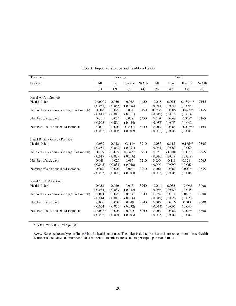
Table 4: Impact of Storage and Credit on Health

Treatment: Storage Credit

Season: All Lean Harvest N(All) All Lean Harvest N(All)

(1) (2) (3) (4) (5) (6) (7) (8)

Panel A: All DistrictsHealth Index -0.00008 0.056 -0.028 6450 -0.048 0.075 -0.130*** 7165

( 0.031) ( 0.036) ( 0.038) ( 0.041) ( 0.059) ( 0.045)1(Health expenditure shortages last month) 0.002 -0.022 0.014 6450 0.023* -0.006 0.042*** 7165

( 0.011) ( 0.016) ( 0.011) ( 0.012) ( 0.016) ( 0.014)Number of sick days 0.014 -0.014 0.028 6450 0.019 -0.063 0.073* 7165

( 0.025) ( 0.020) ( 0.034) ( 0.037) ( 0.056) ( 0.042)Number of sick household members -0.002 -0.004 -0.0002 6450 0.003 -0.005 0.007*** 7165

( 0.002) ( 0.003) ( 0.002) ( 0.002) ( 0.003) ( 0.003)

Panel B: Alfa Omega DistrictsHealth Index -0.057 0.052 -0.111* 3210 -0.053 0.115 -0.165** 3565

( 0.051) ( 0.062) ( 0.061) ( 0.061) ( 0.088) ( 0.069)1(Health expenditure shortages last month) 0.016 -0.022 0.034** 3210 0.021 -0.0009 0.035* 3565

( 0.017) ( 0.029) ( 0.016) ( 0.016) ( 0.019) ( 0.019)Number of sick days 0.048 -0.026 0.085 3210 0.033 -0.111 0.129* 3565

( 0.042) ( 0.031) ( 0.060) ( 0.060) ( 0.090) ( 0.067)Number of sick household members 0.002 -0.002 0.004 3210 0.002 -0.007 0.008** 3565

( 0.003) ( 0.005) ( 0.003) ( 0.003) ( 0.005) ( 0.004)

Panel C: TLM DistrictsHealth Index 0.056 0.060 0.053 3240 -0.044 0.035 -0.096 3600

( 0.034) ( 0.039) ( 0.042) ( 0.056) ( 0.080) ( 0.058)1(Health expenditure shortages last month) -0.011 -0.022 -0.006 3240 0.024 -0.011 0.048** 3600

( 0.014) ( 0.016) ( 0.016) ( 0.019) ( 0.026) ( 0.020)Number of sick days -0.020 -0.002 -0.029 3240 0.005 -0.016 0.018 3600

( 0.024) ( 0.026) ( 0.032) ( 0.044) ( 0.067) ( 0.049)Number of sick household members -0.005** -0.006 -0.005 3240 0.003 -0.002 0.006* 3600

( 0.002) ( 0.004) ( 0.003) ( 0.003) ( 0.004) ( 0.004)

* p<0.1, ** p<0.05, *** p<0.01

Notes: Repeats the analyses in Table 3 but for health outcomes. The index is defined so that an increase represents better health.Number of sick days and number of sick household members are scaled in per capita per month units.

26

Table 5: Impact of Storage and Credit on Seasonal Differences

Treatment: Storage Credit

NGO Districts: All YAO TLM N(All) All YAO TLM N(All)

(1) (2) (3) (4) (5) (6) (7) (8)

Seasonal Difference Index -0.031 -0.067 0.005 1834 -0.050 -0.103* 0.005 2444( 0.036) ( 0.057) ( 0.045) ( 0.033) ( 0.051) ( 0.040)

Log(Staple consumed in kCal) 0.007 -0.024 0.039 1909 0.001 -0.012 0.015 2593( 0.033) ( 0.039) ( 0.052) ( 0.038) ( 0.031) ( 0.072)

Log(Monthly nonfood expenditure) 0.003 0.043 -0.038 1934 -0.066** -0.067 -0.065 2615( 0.040) ( 0.068) ( 0.039) ( 0.032) ( 0.044) ( 0.047)

Log(Reported income) -0.035 -0.052 -0.017 1858 -0.024 -0.087 0.039 2472( 0.064) ( 0.066) ( 0.110) ( 0.054) ( 0.067) ( 0.083)

1(Lacked food last month) -0.036 -0.087 0.015 2150 -0.003 -0.062 0.056 2866( 0.042) ( 0.061) ( 0.057) ( 0.040) ( 0.055) ( 0.057)

* p<0.1, ** p<0.05, *** p<0.01

Notes: Results for seasonal differences. Column 1 reports the results from OLS regressions at the household-cyclelevel where the main regressor is the storage dummy, with district fixed effects and standard errors clustered at thevillage level. Column 1 pools all districts, column 2 only includes Alfa Omega districts and column 3 only includesTLM districts. Each pair of cells reports the coefficient estimate and standard error for the treatment dummy. The fullestimation sample has 2150 households for one post treatment cycle (round 4 minus round 5), including householdsin storage and control villages. The number of observations change for outcomes in logs (more details are in theappendix), the sample sizes pooling all districts are reported in column 4. Columns 5 to 8 report results for creditversus control villages. The full estimation sample has 2866 observations, including households in credit and controlvillages from two post treatment cycles (round 2 minus round 3, round 4 minus round 5). All consumption andincome values are in thousands of Rupiahs (1 USD=9000 Rupiahs), scaled to per capita per month units. The indexis defined so that a decrease represents smaller seasonal fluctuations.

27

reduce seasonal variation and smooth consumption. The effect on the Seasonal Gap Index isstatistically insignificant for all districts but there is a significant decline of 0.103 units (s.e. 0.051)for YAO districts. The reduction seems to be strongest for seasonal differences in the log of monthlynon-food expenditure items which declines by 6.6% (s.e. 3.2%) for all districts. Table 6 reports IVestimates, which are around twice as large as ITT estimates (the take-up rate is 40%).

In summary, both storage and credit increased consumption or income, consistent with eachprogram expanding budget sets, especially in the harvest season. Storage resulted in consumptionincreases in both seasons but with no seasonal smoothing and health effects. Credit had someseasonal smoothing effects but there was also moderately worse reported health in the harvestseason, with no effects on overall health when we pool both seasons.

7.3. Additional TestsHere, we discuss first-stage effects and additional implications as described in Section 4.

Staple salesFor storage, changes in income from harvest sales are statistically insignificant for all districts

but, for YAO districts, sales income increased by 18,000 Rp (s.e. 10,160) in the lean season and by12,000 Rp (s.e. 5,506) in the harvest season (available upon request). This increase in sales incomeis consistent with households selling staples to fund their larger non-food expenditures. We do notdetect changes for storage villages in TLM districts.

For credit, sales income increased by 14,000 Rp (s.e. 5,459 Rp) overall, with increases of17,000 Rp (s.e. 7,314) in the lean season and 12,000 Rp. (s.e. 5,553) in the harvest season forall districts (column 1, Table 7). The increase in sales income in the harvest season is net ofrepayment to the credit program, which, as we discuss further down, suggests that households arenot over-borrowing.

Staple stocksWe do not detect any changes in the overall stock of stored staples in either season for credit

or storage. Measuring the stock of stored maize is hard for reasons described in Section 5 and welack high frequency data on inventory. The increase in sales in the lean seasons for storage villagesin YAO is consistent with expanded inventory in the lean season.

We also conduct a heterogeneous treatment effects analysis that suggests that the storage pro-gram served as a way to improve stock retention. We compare results for households that are exante savings constrained versus households that are not. While this is not necessarily indicative ofthe household’s actual MRT (η), all else equal we predict stronger program effects for householdswith below median retention rates (which are more likely savings constrained). Indeed, Table A5in the appendix shows that the effect is stronger amongst households who are ex ante savings con-strained (the interaction terms with indicators for low-retention-rate households are statisticallysignificant). We explain the heterogeneous treatment effect regressions in the appendix.

This suggests that the main mechanism behind the effects of storage on consumption is analleviation of the savings constraint, as discussed in the model. We cannot construct baselineretention rates for credit since there is no pre-treatment harvest season data.29

29To construct baseline retention rates, we need pre-treatment data for both harvest and lean seasons (round 2 andround 3 for storage).

28

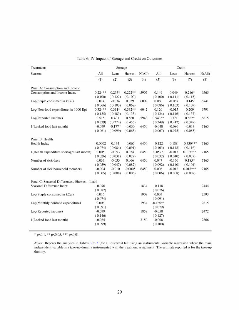
Table 6: IV Impact of Storage and Credit on Outcomes

Treatment: Storage Credit

Season: All Lean Harvest N(All) All Lean Harvest N(All)

(1) (2) (3) (4) (5) (6) (7) (8)

Panel A: Consumption and IncomeConsumption and Income Index 0.224** 0.233* 0.222** 5907 0.149 0.049 0.216* 6565

( 0.100) ( 0.127) ( 0.100) ( 0.100) ( 0.111) ( 0.115)Log(Staple consumed in kCal) 0.014 -0.034 0.039 6009 0.060 -0.067 0.145 6741

( 0.066) ( 0.103) ( 0.068) ( 0.086) ( 0.103) ( 0.109)Log(Non-food expenditure, in 1000 Rp) 0.324** 0.311* 0.332** 6042 0.120 -0.015 0.209 6791

( 0.135) ( 0.183) ( 0.133) ( 0.124) ( 0.146) ( 0.137)Log(Reported income) 0.515 0.431 0.560 5943 0.543** 0.371 0.662* 6615

( 0.339) ( 0.272) ( 0.456) ( 0.249) ( 0.242) ( 0.347)1(Lacked food last month) -0.079 -0.177* -0.030 6450 -0.040 -0.080 -0.013 7165

( 0.061) ( 0.099) ( 0.063) ( 0.067) ( 0.075) ( 0.083)

Panel B: HealthHealth Index -0.0002 0.134 -0.067 6450 -0.122 0.188 -0.330*** 7165

( 0.074) ( 0.084) ( 0.091) ( 0.103) ( 0.148) ( 0.116)1(Health expenditure shortages last month) 0.005 -0.053 0.034 6450 0.057* -0.015 0.105*** 7165

( 0.026) ( 0.038) ( 0.027) ( 0.032) ( 0.040) ( 0.037)Number of sick days 0.033 -0.033 0.066 6450 0.047 -0.160 0.185* 7165

( 0.059) ( 0.047) ( 0.082) ( 0.092) ( 0.140) ( 0.104)Number of sick household members -0.004 -0.010 -0.0005 6450 0.006 -0.012 0.018*** 7165

( 0.005) ( 0.008) ( 0.005) ( 0.006) ( 0.008) ( 0.007)

Panel C: Seasonal Differences, |Harvest - Lean|Seasonal Difference Index -0.070 1834 -0.118 2444

( 0.082) ( 0.076)Log(Staple consumed in kCal) 0.016 1909 0.003 2593

( 0.074) ( 0.091)Log(Monthly nonfood expenditure) 0.006 1934 -0.160** 2615

( 0.091) ( 0.079)Log(Reported income) -0.079 1858 -0.058 2472

( 0.146) ( 0.127)1(Lacked food last month) -0.085 2150 -0.008 2866

( 0.099) ( 0.100)

* p<0.1, ** p<0.05, *** p<0.01

Notes: Repeats the analyses in Tables 3 to 5 (for all districts) but using an instrumental variable regression where the mainindependent variable is a take-up dummy instrumented with the treatment assignment. The estimate reported is for the take-updummy.

29

Social and behavioral considerationsWe examine each program through the social and behavioral lens described in Section 4. We

investigate a proxy for social pressures to share–the need to contribute to neighbors’ festival expen-ditures. Storage participants could circumvent this constraint by committing to store harvest forthe lean season. To test this, we calculate the share of a household’s annual festival expendituresthat is used for neighbors’ festivities. We find that households in YAO storage villages report a 10p.p. reduction (s.e. 3.7 p.p.) in the share of festival expenditures spent on others. This reductionfor YAO villages is consistent with the mechanism described above, where commitment (formalor informal) associated with storage raised storage retention rates, γ .

We also find similar results for credit–for YAO villages, there was a 9.1 p.p reduction (s.e. 4.4p.p.) in the share spent on others. This suggests that both programs play some role in reducingvisibility of assets and consequent vulnerability to social pressures.

For credit, we see no evidence of over-borrowing. First, we find that loans are always repaid,though in some cases after a permitted delay due to harvest failures. Second, there are increasedsales in the harvest season. Since repayment is in-kind, these sales are indicative of surplus stockthat must go towards additional consumption or savings.

Other budget set effectsIn the model, the budget constraint (equation 2) included only agricultural endowments and

assumed away other sources of revenue that could give rise to income effects, including wagesand private transfers (gifts and remittances). We see that neither program affected other budget setfactors, providing further support that the income effects above are directly due to the programs’effect on the MRT of staples. One concern is that the null staple effects might arise because ourtransfers are exactly offset or crowded out by other income sources. Table 7 shows that neitherprogram affected transfers or wage income. Another concern is that staple consumption mighthave increased at the household level but not at the per capita level if household size increased butthere are no effects on household size.

7.4. Cost Benefit AnalysisThe main cost component for storage includes the procurement costs to purchase the storage

equipment. These represent direct transfers to households. For storage, the average procurementcost per eligible household was 134,553 Rp. We calculate this by first dividing the total procure-ment cost per NGO by the total number of eligible households, and then averaging across bothNGOs. For credit, the average procurement cost was 325,845 Rp. This was used to purchase andtransport the first loan disbursements to the credit villages.

The benefit-to-cost ratio for storage, using annualized benefits and average procurement costs,is 43% (=58,000 Rp/134,553 Rp). To calculate annualized benefits for storage, we use the resultthat storage had statistically significant effects on ln(Non-food expenditures) in both harvest andlean seasons (Table 3).30

30The ITT estimate of the treatment effect on non-food expenditure levels for households is 29,000 Rp. The annual-ized benefit, then, is 58,000 Rp. We repeated the exercise using expenditure levels for households instead of per capitaunits since program participation is at the household level (this includes observations with zero non-food expenditures,which is more conservative).

30

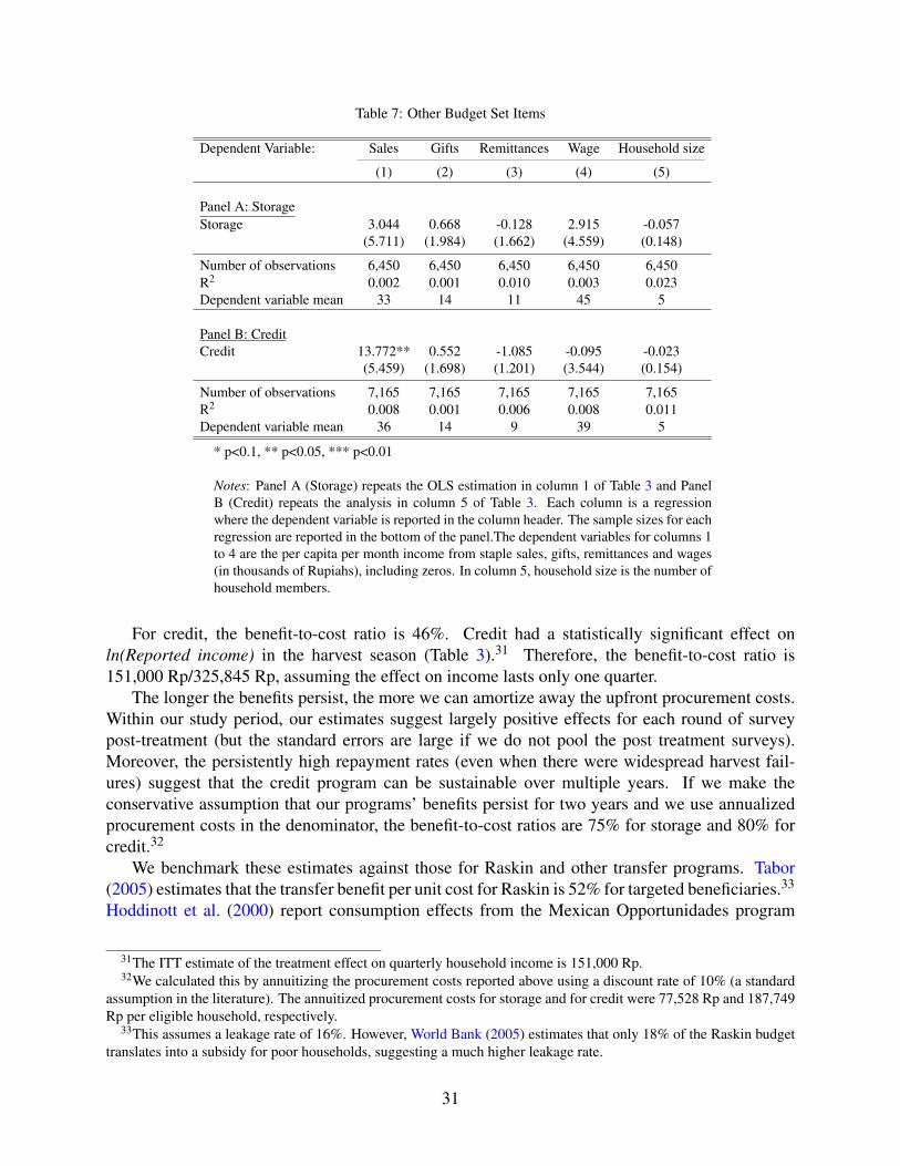
Table 7: Other Budget Set Items

Dependent Variable: Sales Gifts Remittances Wage Household size

(1) (2) (3) (4) (5)

Panel A: StorageStorage 3.044 0.668 -0.128 2.915 -0.057

(5.711) (1.984) (1.662) (4.559) (0.148)

Number of observations 6,450 6,450 6,450 6,450 6,450R2 0.002 0.001 0.010 0.003 0.023Dependent variable mean 33 14 11 45 5

Panel B: CreditCredit 13.772** 0.552 -1.085 -0.095 -0.023

(5.459) (1.698) (1.201) (3.544) (0.154)

Number of observations 7,165 7,165 7,165 7,165 7,165R2 0.008 0.001 0.006 0.008 0.011Dependent variable mean 36 14 9 39 5

* p<0.1, ** p<0.05, *** p<0.01

Notes: Panel A (Storage) repeats the OLS estimation in column 1 of Table 3 and PanelB (Credit) repeats the analysis in column 5 of Table 3. Each column is a regressionwhere the dependent variable is reported in the column header. The sample sizes for eachregression are reported in the bottom of the panel.The dependent variables for columns 1to 4 are the per capita per month income from staple sales, gifts, remittances and wages(in thousands of Rupiahs), including zeros. In column 5, household size is the number ofhousehold members.

For credit, the benefit-to-cost ratio is 46%. Credit had a statistically significant effect onln(Reported income) in the harvest season (Table 3).31 Therefore, the benefit-to-cost ratio is151,000 Rp/325,845 Rp, assuming the effect on income lasts only one quarter.

The longer the benefits persist, the more we can amortize away the upfront procurement costs.Within our study period, our estimates suggest largely positive effects for each round of surveypost-treatment (but the standard errors are large if we do not pool the post treatment surveys).Moreover, the persistently high repayment rates (even when there were widespread harvest fail-ures) suggest that the credit program can be sustainable over multiple years. If we make theconservative assumption that our programs’ benefits persist for two years and we use annualizedprocurement costs in the denominator, the benefit-to-cost ratios are 75% for storage and 80% forcredit.32

We benchmark these estimates against those for Raskin and other transfer programs. Tabor(2005) estimates that the transfer benefit per unit cost for Raskin is 52% for targeted beneficiaries.33

Hoddinott et al. (2000) report consumption effects from the Mexican Opportunidades program

31The ITT estimate of the treatment effect on quarterly household income is 151,000 Rp.32We calculated this by annuitizing the procurement costs reported above using a discount rate of 10% (a standard

assumption in the literature). The annuitized procurement costs for storage and for credit were 77,528 Rp and 187,749Rp per eligible household, respectively.

33This assumes a leakage rate of 16%. However, World Bank (2005) estimates that only 18% of the Raskin budgettranslates into a subsidy for poor households, suggesting a much higher leakage rate.

31

implying a benefit-to-cost ratio of 77%.34 Importantly, rice subsidies, cash and in-kind transfersare financed by per-period transfers while our programs are financed from one-time costs.

In summary, our benefit-to-cost estimates for storage and credit are 43% and 46% respectively.Amortizing procurement costs over 2 years increases our benefit-to-cost ratios to 75% for storageand 80% for credit. These calculations have the advantage of being comparable to other papers butignore other effects (such as food shortages, health and seasonal smoothing effects) that are harderto monetize without estimating household preferences. For example, for credit, these benefits willhave to weighed against the negative health effects in the harvest season. Another caveat is thatthese calculations ignore implementation costs. We discuss this in the appendix.

7.5. Limitations and Lessons for Future WorkWe discuss several limitations of our research design and lessons for future work on season-

ality. In particular, we are concerned about implications for consumption in scaled-up credit andstorage programs, and how new data could better unpack the channels through which each programoperates.

Timeliness and harvest risks in a finite study periodTiming is important in a seasonal study because even slight delays could be costly. For ex-

ample, we had initially planned to distribute storage equipment in the first harvest season (April2009), which would allow households to store over two harvest seasons. The equipment arrivedfour months late, but we had to wait till the following maize harvest (April 2010) for householdsto start storing staples. This was also the only harvest season where we had data for the full agri-cultural cycle (which we need to construct absolute seasonal differences within a cycle). Thisexample illustrates how a seemingly short delay of 4 months resulted in us losing two roundsof post treatment data. Also, delays in seasonal surveys meant we were likely measuring someseasonal outcomes with recall error, which may make it harder to measure seasonal differences.

Harvest risks further exacerbated the problems above. These harvest failures tend to be relatedto weather patterns that are widespread, covering entire districts. Since we focus on rain-fed, staplesubsistence farmers who only have one harvest a year, this means we only observe three harvestseasons in our three-year study, and any widespread harvest failures would reduce the statisticalpower of the study substantially (since each harvest failure will also have implications for thefollowing lean season survey). This suggests it would be useful to stratify by regions (so thatresults are internally valid within regions), across multiple regions (to insure against widespreadharvest risk) and have a longer study period.

General equilibrium price effectsWe do not find statistically significant general equilibrium price effects because we only treat

18 villages in each district and the program is of limited duration. A sufficiently large expansion ofthe programs should ultimately reduce the staple supply in the harvest season and raise the staplesupply in the lean season. This will translate into a drop in lean season staple prices and a rise inharvest season staple prices.

While these general equilibrium effects arise out of improved storage or credit markets, welfareeffects for some households will be ambiguous. For example, consider a household that had access

34Calculated using benefits valued at 197 pesos per month and consumption effects of 151 pesos.

32

to a high-returns storage technology prior to the program and therefore did not experience a directexpansion of its budget set through food credit or food storage. In the short run, such a householdwill be unaffected by the programs. However, as a result of general equilibrium effects, sincestaples are expected to get cheaper in the lean season, lean season non-food consumption will getmore expensive (relative to staples). If the household has a preference for lean season non-foodconsumption (that it funds through saved staples), it will be made worse off.

Measurement issuesAs discussed above, inventory was hard to measure precisely due to the nature of maize storage,

especially in control villages. Also, whether inventory was measured before or after consumptionand sales mattered crucially. More frequent and precisely timed measures of inventory would help.Second, it would have been useful to collect more data on the price at which staples were sold.This would help us decompose the result that each program raised income from staple sales, so wecould learn to what extent this was driven by changes in the quantity of staples sold rather thanvariation in prices. Third, as discussed earlier, this study would benefit from more detailed data onthe consumption of other food and non-food items.

Finally, we lack statistical power in variables related to seasonality. By definition, seasonaldifferences are defined for each agricultural cycle instead of by season. For example, for thestorage treatment, we only had one post treatment cycle (rounds 4 and 5), which limited the samplesize. Due to our budget constraint, we faced a significant trade-off between spatial and time-seriesvariation. Ultimately, we chose to have a larger cross-section (to insure against regional harvestrisks) instead of a longer time series (to have more post treatment cycles). In the future, it would beuseful to have a larger sample or to collect data on other seasonal outcomes that are measured withless noise. This would also aid in precision for other outcomes, since consumption and income areknown to be measured with error. Having more power would allow us to trace out dynamic effectsby rounds.

8. Conclusion

This paper focuses on staple farmers in West Timor who use low-MRT technologies to transferassets between harvest and lean seasons. The seasonal storage program increased the retentionrate of stored staples and the seasonal credit program allowed households to borrow cheaply in thelean season. By introducing new technologies to raise the harvest-to-lean season MRT for staplefarmers, these programs implicitly subsidized the relative price of lean season consumption.

The storage program increased non-food consumption in the harvest and lean seasons, mea-sured over a relatively short span of time. But storage had no effects on health or outcomes relatedto seasonal fluctuations. Overall, benefits of the storage program derived from both higher returnsto savings and reduced social pressures.

The credit program increased reported income with no decreases in consumption. Credit alsoincluded more tools for insuring against risk. Participants showed reduced gaps in seasonal differ-ences, especially in YAO villages. However, credit led to some deterioration in health in the harvestseason. Repayment rates were consistently high except during harvest failures and there was noevidence of over-borrowing. For each program, we find some evidence of increased staple sales,but no evidence of changes in staple inventory. This is likely due to a combination of theoreticallyambiguous predictions and data limitations.

33

Both storage and credit led to increases in non-food consumption or reported income but hadnull effects on staple consumption. This is notable given both programs’ focus on staple food,and transaction costs related to the remoteness of program villages. This suggests staple farmersin our study could be close to staple food satiation, but still benefit from the higher MRT throughexpanded budget sets.

Since the programs incur front-loaded costs and have recurring financial benefits, our cost-benefit analysis argues that they provide a cost-effective way to help farmers adapt to seasonality.Amortizing procurement costs over 2 years results in benefit-to-cost ratios of 75% for storage and80% for credit. In future work, it would be interesting to see if a longer-term analysis would raisethe implied cost-effectiveness of the programs.

The food storage and food credit programs, when modified with caution, could inform food pol-icy elsewhere. Rudimentary food storage technologies are prevalent in several agrarian economies,and the introduction of improved storage (used directly for storage programs or indirectly for creditprograms) could similarly expand budget sets for other poor households. Our research comes withsome caveats and suggestions for ongoing investigation.

Unlike regular subsidies on staples, these programs are of less immediate value to non-farminghouseholds whose incomes are not seasonal and not in-kind. Unless such households could repli-cate the behavior of farming households by conducting basic transactions using staples, they cannottake advantage of the lean season subsidy implicit in food storage and food credit. This also high-lights an inherent strength and weakness of in-kind seasonal programs targeted at staple farmers.By raising the MRT of staple crops, the programs target the underlying source of seasonal frictionsin our setting (high depreciation rate of staples). However, this implies that treatment effects areconditional on output, which matters in an environment with significant harvest risks.

34

References

Afzal, U., d’Adda, G., Fafchamps, M., Quinn, S., Said, F., 2014. Two Sides of the Same Rupee?Comparing Demand for Microcredit and Microsaving in a Framed Field Experiment in RuralPakistan. CSAE Working paper 2014-32.

Ahmed, A.U., Quisumbing, A.R., Nasreen, M., Hoddinott, J.F., Bryan, E., 2010. ComparingFood and Cash Transfers to the Ultra-Poor in Bangladesh. IFPRI Research Monograph 163.Washington, DC: IFPRI.

Alderman, H., Garcia, M., 1993. Poverty, Household Food Security, and Nutrition in Rural Pak-istan. Research reports 96. International Food Policy Research Institute (IFPRI).

Alderman, H., Sahn, D.E., 1989. Understanding the Seasonality of Employment, Wages, andIncomes, in: Sahn, D. (Ed.), Seasonal Variability in Third World Agiculture. Johns HopkinsUniversity Press, Baltimore, MD.

Angelucci, M., Attanasio, O., 2013. The Demand for Food of Poor Urban Mexican Households:Understanding Policy Impacts Using Structural Models. American Economic Journal: Eco-nomic Policy 5, 146–205.

Ashraf, N., Karlan, D., Yin, W., 2006. Tying Odysseus to the Mast: Evidence from a CommitmentSavings Product in the Philippines. The Quarterly Journal of Economics 121, 635–672.

Attanasio, O., Battistin, E., Mesnard, A., 2012. Food and Cash Transfers: Evidence from Colom-bia. The Economic Journal 122, 92–124.

Baland, J.M., Guirkinger, C., Mali, C., 2011. Pretending to Be Poor: Borrowing to Escape ForcedSolidarity in Cameroon. Economic Development and Cultural Change 60, 1–16.

Banerjee, A.V., Duflo, E., 2007. The Economic Lives of the Poor. The Journal of EconomicPerspectives 21, 141–168.

Barrett, C., 2002. Food Security and Food Assistance Programs. Handbook of Agricultural Eco-nomics 2, 2103–2190.

Basu, K., 2014. Commitment Savings in Informal Banking Markets. Journal of DevelopmentEconomics 107, 97–111.

Beaman, L., Karlan, D., Thuysbaert, B., 2014. Saving for a (not so) Rainy Day: A RandomizedEvaluation of Savings Groups in Mali. Working paper.

Behrman, J., Foster, A., Rosenzweig, M., 1997. The Dynamics of Agricultural Production and theCalorie–Income Relationship. Journal of Econometrics 77, 187–207.

Behrman, J.R., 1988. Nutrition, Health, Birth Order and Seasonality: Intrahousehold Allocationamong Children in Rural India. Journal of Development Economics 28, 43–62.

Besley, T., Kanbur, R., 1990. The Principles of Targeting. Policy Research Working Paper Series385. World Bank.

35

Bryan, G., Chowdhury, S., Mobarak, A.M., 2014. Underinvestment in a Profitable Technology:The Case of Seasonal Migration in Bangladesh. Econometrica 82, 1671–1748.

Burke, M., 2014. Selling Low and Buying High: An Arbitrage Puzzle in Kenyan Villages. Workingpaper.

Chaudhuri, S., Paxson, C., 2002. Smoothing Consumption Under Income Seasonality: BuyerStocks vs. Credit Markets. Discussion Paper Series No. 0102-54, Department of Economics,Columbia University.

Deaton, A., 1991. Saving and Liquidity Constraints. Econometrica 59, 1221–1248.

Devereux, S., Sabates-Wheeler, R., Longhurst, R., 2012. Seasonality, Rural Livelihoods and De-velopment. Earthscan, London, UK.

Devereux, S., Vaitla, B., Swan, S.H., 2008. Seasons of Hunger: Fighting Cycles of StarvationsAmong the World’s Rural Poor. Pluto Press, London, UK.

Dréze, J., Sen, A., Hussain, A., 1995. The Political Economy of Hunger: Selected Essays. OxfordUniversity Press, Oxford, UK.

FAO, 2003. Special Report, Crop and Food Supply Assessment Mission to Timore Leste. Foodand Agriculture Organization and Food and United Nations World Food Programme.

Fink, G., Jack, B.K., Masiye, F., 2014. Seasonal Credit Constraints and Agricultural Labor Supply:Evidence From Zambia. NBER Working Paper 20218.

Fox, J., 1977. Harvest of the Palm. Harvard University Press, Cambridge, MA.

Gelay, 2008. Rice Bank: Breaking the Poverty Cycle. URL: http://www.vast-bhutan.org/2008/06/19/rice-bank-breaking-the-poverty-cycle/.

Handa, S., Mlay, G., 2006. Food Consumption Patterns, Seasonality and Market Access in Mozam-bique. Development Southern Africa 23, 541–560.

Hidrobo, M., Hoddinott, J., Peterman, A., Margolies, A., Moreira, V., 2014. Cash, Food, or Vouch-ers? Evidence from a Randomized Experiment in Northern Ecuador. Journal of DevelopmentEconomics 107, 144–156.

Hoddinott, J., Skoufias, E., Washburn, R., 2000. The Impact of PROGRESA on Consumption: AFinal Report. Technical Report. International Food Policy Research Institute.

Jensen, R., Miller, N., 2008. Giffen Behavior and Subsistence Consumption. American EconomicReview 98, 1553–1577.

Jensen, R.T., Miller, N.H., 2011. Do Consumer Price Subsidies Really Improve Nutrition? Reviewof Economics and Statistics 93, 1205–1223.

Jha, S., Ramaswami, B., 2010. How Can Food Subsidies Work Better? Answers from India andthe Philippines. Economics Working Paper Series 221. Asian Development Bank.

36

Johnston, D., Morduch, J., 2008. The Unbanked: Evidence from Indonesia. The World BankEconomic Review 22, 517–537.

Khandker, S., 2012. Seasonality of Income and Poverty in Bangladesh. Journal of DevelopmentEconomics 97, 244–256.

Khandker, S., Khaleque, M.A., Samad, H.A., 2011. Can Social Safety Nets Alleviate SeasonalDeprivation? Evidence from Northwest Bangladesh. World Bank Policy Research WorkingPaper Series .

Khandker, S., Khalily, M., Samad, H.A., 2010. Seasonal and Extreme Poverty in Bangladesh:Evaluating an Ultra-Poor Microfinance Project. World Bank Policy Research Working PaperSeries 5331 .

Khandker, S.R., Mahmud, W., 2012. Seasonal Hunger and Public Policies: Evidence from North-west Bangladesh. World Bank Publications, Washington, DC.

Kling, J.R., Liebman, J.B., Katz, L.F., 2007. Experimental Analysis of Neighborhood Effects.Econometrica 75, 83–119.

Lines, T., 2011. The Potential Establishment of Emergency Food Reserve Funds. UNCTAD Spe-cial Unit on Commodities Working Paper Series on Commodities and Development Discussionpaper, 3.

Mohan, V., Takada, M., Kalavakonda, V., Banerjee, S.S., Shah, P., 2007. Community ManagedFood Security Enterprises in Andhra Pradesh, India. Technical Report. Livelihoods LearningSeries 1, Note 4. World Bank: Washington, DC.

Olken, B., 2006. Corruption and the Costs of Redistribution:Micro Evidence from Indonesia.Journal of Public Economics 90, 853–870.

Olken, B., 2007. Monitoring Corruption: Evidence from a Field Experiment in Indonesia. Journalof Political Economy 115, 200–219.

Paxson, C., 1993. Consumption and Income Seasonality in Thailand. Journal of Political Economy101, 39–72.

Pinstrup-Anderson, P., Jaramillo, M., 1989. The Impact of Drought and Technological Changein Rice Production on Intrayear Fluctuations in Food Consumption: The Case of North Ar-cot, India, in: Sahn, D. (Ed.), Seasonal Variability in Third World Agriculture. Johns HopkinsUniversity Press, Baltimore, MD.

Pitt, M.M., Khandker, S.R., 2002. Credit Programmes for the Poor and Seasonality in RuralBangladesh. Journal of Development Studies 39, 1–24.

Ravallion, M., 1987. Markets and Famines. Clarendon Press, London, UK.

Sahn, D., 1989. Seasonal Variability in Third World Agriculture: the Consequences for FoodSecurity. Baltimore: John Hopkins University Press.

37

Sen, A., 1981a. Ingredients of Famine Analysis: Availability and Entitlements. Quarterly Journalof Economics 96, 433–464.

Sen, A., 1981b. Poverty and Famines: An Essay on Entitlement and Deprivation. Oxford Univer-sity Press, New York, NY.

Stephens, E.C., Barrett, C.B., 2011. Incomplete Credit Markets and Commodity Marketing Be-haviour. Journal of Agricultural Economics 62, 1–24.

Tabor, S., 2005. RASKIN: Evolution of a Transfer Program. Technical Report. The Bureau ofLogistic Reports, Indonesia.

Townsend, R., 1994. Risk and Insurance in Village India. Econometrica 62, 539–591.

Trinugroho, I., Sutomo, Riani, A.L., 2011. The Efficiency of Public Service Obligation for FoodSubsidy in Indonesia: Review of Cost Structure Analysis. Perspectives of Innovations, Eco-nomics & Business 7, 45–47.

World Bank, 2005. Feeding Indonesia. Technical Report. World Bank.

Zeller, M., 2001. The Safety Net Role of Microfinance for Income and Consumption Smoothing,in: Lustig, N. (Ed.), Shielding the Poor: Social Protection in the Developing World. BrookingsInstitution Press, pp. 217–238.

Zeller, M., Schrieder, G., von Braun, J., Heidhues, F., 1997. Rural Finance for Food Security of thePoor: Implications for Research and Policy. Food Policy Review 4.. International Food PolicyResearch Institute. Washington, DC.

38