Embed Size (px)
Citation preview

Pnevmatikos-Niavis-Polyzos, 82-93
MIBES ORAL Larissa, 8-10 June 2013 82
Evaluating Greek economic sectors' regional
dynamics during the pre and in-crisis period
Triantafyllos Pnevmatikos
University of Thessaly, School of Engineering,
Department of Planning and Regional Development
Spyros Niavis
University of Thessaly, School of Engineering,
Department of Planning and Regional Development
Serafeim Polyzos
University of Thessaly, School of Engineering,
Department of Planning and Regional Development
Abstract
As economic recession is still present in Greece, economic sectors are
strongly influenced by the negative growth rates of Greek economy. The
process of recovery should be primarily based on the strengthening of
the most competitive sectors. The present paper aims at the
identification of the sectors that should constitute the growth
engines of the Greek economy. Analysis does not only target on the
national level, but it also takes into account the dynamics of sectors
in Greek prefectures. The present paper focuses both on the pre-crisis
and in-crisis period as the estimations concern the years 2005 and
2010. For the identification of sectors’ dynamics, an input – output
analysis is adopted and the size of regional multipliers for the Greek
prefectures (NUTS III) is estimated. Then, the observed differences
and the changes amongst the multipliers for the prefectures and
sectors are analyzed and evaluated. Additionally, the values of
regional multipliers of the most dynamic sectors are implemented as
the dependent variable in a regression analysis in which a set of
socio-economic and spatial factors of Greek prefectures are used as
the independent variables. By doing so, we are able to capture the
relationship among the characteristics of each prefecture and the
dynamics of its economic sectors.
Keywords: Input-Output Analysis, Regional multipliers, Regional
Development, Tobit regression, Greece
JEL classification: R15, O33, O52, C240
Introduction
Input-output I-O analysis as an economic modeling technique aims at
understanding the interactions between productive sectors, producers
and consumers within an economy. It is a powerful tool for the
estimation of magnitude of transactions occurred between different
sectors of an economy, providing useful overview of the structure of
it (Polyzos and Sofios, 2008). An input-output table includes the
flows of products from each sector considered as a producer to each of
the sectors considered as consumers (Miller and Blair, 2009). Several
I-O techniques have been developed and are widely used worldwide for
measuring diverse elements and entities such as gross regional
product, household consumption and employment generation.

Pnevmatikos-Niavis-Polyzos, 82-93
MIBES ORAL Larissa, 8-10 June 2013 83
Other analytical techniques such as shift-share and location quotient
analyses, econometric and statistical models have also been developed
for measuring relevant regional economic aspects. These tools provide
useful insights into the structure of regional economies and their
trajectories of change over time. The various analytical techniques
rely heavily upon quantitative methods and their use for analyzing
regional economies has certain limitations (Polyzos and Sofios, 2008).
By using Input-Output (I-O) Analysis we can study the structural
changes within a national or regional economy, since it provides the
tools that are necessary in order to evaluate industries, including
their relationships to the rest of the economy and the effects of
international or interregional trade on those relationships. Moreover,
it provides the scientific base for the product and employment
multipliers estimation and thereby the evaluation of each applied
economic policy. Although input-output models were firstly applied at
a nation-wide level, the models were modified in order to cover
different spatial units, such as regions. The extension of the
national-level models led to the creation of a set of regional input-
output models.
In this paper, we regionalize the national Input Output tables and
estimate the regional multipliers of Greek Prefectures. Thus, we
analyze the structural changes in the regional economy for the period
2005 to 2010 using national input-output tables provided by National
Statistical Services of Greece. Additionally, a regression model is
formulated in order to estimate the relationship among the values of
the regional multipliers and several features of regional economy.
The structure of the remainder paper is as follows. In the next
section the methods of I-O tables’ regionalization are described and
evaluated. Then, the Input – Output technical coefficients are
estimated by using the LQ’s technique for the 51 Greek prefectures.
Moreover, an analysis of multipliers’ changes is performed and the
values of multipliers are regressed with a set of socio-economic and
spatial factors of each prefecture. The paper concludes by drawing
some general remarks derived from the preceding analysis.
Input - Output technical coefficients’ regionalization
The general equation of the I-O analysis for n productive sectors of
an economy is the following (Miller and Blair, 2009):
X=(I-A)-1f (1)
where, X is the total output of economy, Α denotes the technical
coefficients matrix, and f is the final demand of economy.
The common methods that are used to develop a regional I-O table can
be distinguished in three basic categories: (a) The survey methods,
(b) The non-survey methods and (c) The partial survey or hybrid
methods. The central task of these methods, mainly of the two last
ones, is the adaptation of the technical coefficients of a national I-
O table in order to highlight features of the analyzed regional
economy. With the survey method, primary data concerning the regional
intra-sectoral transactions are used for the construction of the
regional I-O table. This procedure is rarely used at the regional
level since it is costly and time-consuming.

Pnevmatikos-Niavis-Polyzos, 82-93
MIBES ORAL Larissa, 8-10 June 2013 84
The non-survey methods, based on the application of various techniques
for the modification of the national technical coefficients of I-O
table in regional ones, are used more frequently. A number of non-
survey techniques for regionalization of national coefficients through
adjustments are based entirely on published regional statistical data
about employment, output, added value and income.
The third category includes the hybrid techniques which combine the
survey and non-survey methods through superior statistical data and
information obtained from small scale surveys. The methods of this
category have expanded beyond the limitations of non-survey approaches
and the prohibitive costs of survey methods assuring a compromise
between accuracy and required recourses.
In this paper a non-survey method will be implemented, in order to
estimate the regional technical coefficients of I-O analysis for Greek
Prefectures (NUTS III). Before applying the method to the Greek case,
a brief description of the main techniques that belong to the second
category will be preceded.
The assumptions made by non-survey methods concern existing
differences between a regional and a national economy, despite the
commonly assumed similarity of the production technology. The
techniques that have been developed focus on the estimation of input
and trade coefficients and less on technical coefficients because the
assumption of identical technology. According to many empirical
findings the regional purchase coefficients used to scale down the
inputs are more important in determining the accuracy of the model
than is the assumption of similarity of the production technology
(Kuhar et al., 2009). The basic data or regional indices used by these
methods concern location quotient, regional supply percentages,
supply-demand pool approach, regional purchase coefficients, etc. The
majority of these methods are based on the location quotient index. A
brief description of the most important approaches belonging in this
category takes place below.
(a) A way to modify the national coefficients in regional ones is by using Simple Location Quotients (SLQ). The SLQ for sector i in region
r is defined as:
r r
r i
i N N
i
Q / QSLQ
Q / Q (2)
where r
iQ and
rQ denote output (or alternatively employment) of sector i
in region r and total output of all sectors in region r, respectively,
and let N
iQ and
NQ denote these totals at the national level. When
r
iSLQ 1, the sector i is more localized or concentrated in region r
than in the nation as a whole, and it is able to satisfy the regional
demand requirements for its products. In this case, the regional
coefficient is assumed r N
ij ijα α and the same assumption holds if
r
iSLQ 1. Conversely, if r
iSLQ 1, then the sector i is less localized
or less concentrated in region r than in the nation as a whole.
Consequently, the region needs to import products from other regions
in this sector in order to satisfy the whole regional demand
requirements and r N r
ij ij iSLQα α (Miller and Blair, 2009).

Pnevmatikos-Niavis-Polyzos, 82-93
MIBES ORAL Larissa, 8-10 June 2013 85
(b) The above modification has been improved by using the Cross-
Industry Location Quotient (CILQ). The CILQ compares the share of the
selling industry’s output of the region to the national with that of
the purchasing industry in the region to the national and it is
formulated as:
i
ij
j
SLQCILQ
SLQ (3)
When CILQij> 1, the regional selling sector i can supply all the
requirements of the regional purchasing sector j and the sector i has
a greater share in sectoral national output than the sector j. In this
case, no adjustment is needed and the regional technical coefficient
and the regional imports coefficient are identical with the national
ones. Similarly, no adjustment is needed when CILQij=1. If CILQij<1, the
regional technical coefficient is adjusted downward with the product
of the national coefficient and the computed CILQij.
(c) Round (1978) proposed a new formula using the semilogarithmic
quotient (RLQ). In this new location quotient the selling and
purchasing sectors are considered as in the case of CILQ, but also the
relative sizes of region and nation are added. The RLQ is formulated
as:
i
ij
2 j
SLQRLQ
log(1 SLQ ) (4)
Thus, r N r
ij ij iRLQα α .
(d) Another formula has been developed by Flegg et al. (1995) and
Flegg and Webber (1997), in order to overcome some weaknesses of the
previous ones. They had as starting point the fact that the SLQ and
CILQ provide an alternative way of estimating the relevant trading
coefficients. Trading coefficients measuring the proportion of a
commodity supplied from within the region depend on the next
variables: (a) the relative size of the supplying sector, (b) the
relative size of the purchasing sector, (c) the relative size of the
region (Kuhar et al., 2009).
In the formula proposed by Flegg et al. (1995), the three variables
are captured and the formula is defined as follows:
ij ij
FLQ CILQ λ (5)
In equation (5), λ is the weighting measure of the regions’ relative
size and it is estimated as follows:
r
i δ
2 N
i
Qλ [log(1 ]
Q with 0≤δ≤1 and 0≤λ≤1 (6)
where, δ is the weighting parameter based on the size of region. Then,
r r n
ij ij ijα FLQ α for r
ijFLQ <1
r n
ij ijα α for
r
ijFLQ ≥1
(7)

Pnevmatikos-Niavis-Polyzos, 82-93
MIBES ORAL Larissa, 8-10 June 2013 86
Flegg and Weber (2000) developed another augmented formula, which
allows for r N
ij ijα α and it is defined as:
ij ij 2 j
AFLQ FLQ [log(1 SLQ )] for j
SLQ >1
ij ij
AFLQ FLQ for j
SLQ ≤1 (8)
Regional multipliers in Greek prefectures for the years
2005 and 2010
This section focuses on the measurement of the technical coefficients
for the Greek prefectures at years 2005 and 2010 using the FLQ method
described by the equations (5), (6) and (7).
According to the references (Flegg and Webber, 2000; Miller and Blair,
2009), the coefficient δ is usually defined arbitrarily and its value
is specified close to 0.3. In this article, the technical coefficients
were calculated by using δ = 0.1, 0.2 and 0.3. The results show that
δ=0.1 is the most suitable value in order to calculate technical
coefficients and multipliers at prefecture level.
By using the matrices of technical coefficients, we estimate the
product multipliers for the industries of the Greek prefectures
according to the equation,
n
j ij
i 1
OM b , where j
OM is the product
multiplier of the industry j and bij are the elements of Leontief
inverse matrix. The changes of the multipliers will show which
industries have been affected most by the economic crisis and which
industries should constitute the growth engines for the economic
recovery of the Greek economy.
The results indicate that the industries that present the highest
product multipliers at Greece in 2005 are the following:
constructions, professional, scientific and technical activities, and
accommodation and food service activities. In 2010, industries of
Greek economy such as constructions, professional, scientific and
technical activities, administrative and support service activities,
and human health and social work activities have the highest product
multipliers.
By examining the dominant industries at prefecture level, it is
evident that in 2005 the product multipliers in the constructions
industry show high values in prefectures such as Attiki, Thessaloniki,
Kavala, Evoia and Imathia. In 2010, the most important product
multipliers in the constructions industry are observed in prefectures
of Drama, Serres, Fthiotida, Attiki and Thessaloniki.
The professional, scientific and technical activities constitute a
growing industry of the Greek economy that presents high values of
product multipliers in prefectures such as Attiki, Thessaloniki,
Achaia, Ioannina, Kavala, Voiotia, Fthiotida.
As far as the accommodation and food service activities, it is
realized that prefectures of Attiki, Larisa, Voiotia, Thessaloniki and
Imathia get major multiplier effects both in 2005 and 2010. It is
worth noting that there is important reduction at the product
multipliers values in 2010. Moreover, the island prefectures appear
low product multipliers values in this industry.
Pnevmatikos-Niavis-Polyzos, 82-93
MIBES ORAL Larissa, 8-10 June 2013 87
Prefectures including major urban centers (Attiki, Thessaloniki,
Larissa, Achaia, Serres, Fthiotida, Korinthia, Evoia etc.) show high
product multipliers values in industries of the tertiary sector such as administrative and support service activities and human health and
social work activities both in 2005 and 2010.
Finally, prefectures of Magnisia, Thessaloniki, Korinthia, Attiki and
Kavala get the highest product multipliers values in the primary
sector (agriculture, forestry and fishing).
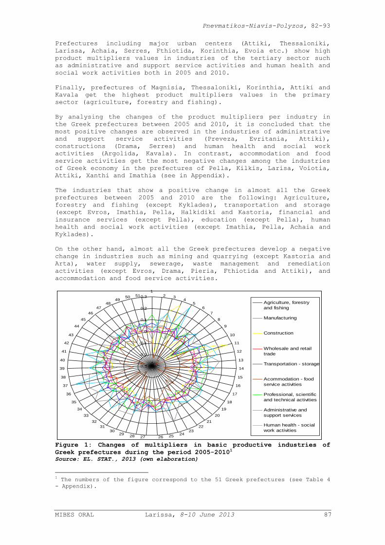
By analysing the changes of the product multipliers per industry in
the Greek prefectures between 2005 and 2010, it is concluded that the
most positive changes are observed in the industries of administrative
and support service activities (Preveza, Evritania, Attiki),
constructions (Drama, Serres) and human health and social work
activities (Argolida, Kavala). In contrast, accommodation and food
service activities get the most negative changes among the industries of Greek economy in the prefectures of Pella, Kilkis, Larisa, Voiotia,
Attiki, Xanthi and Imathia (see in Appendix).
The industries that show a positive change in almost all the Greek
prefectures between 2005 and 2010 are the following: Agriculture,
forestry and fishing (except Kyklades), transportation and storage
(except Evros, Imathia, Pella, Halkidiki and Kastoria, financial and
insurance services (except Pella), education (except Pella), human
health and social work activities (except Imathia, Pella, Achaia and
Kyklades).
On the other hand, almost all the Greek prefectures develop a negative
change in industries such as mining and quarrying (except Kastoria and
Arta), water supply, sewerage, waste management and remediation
activities (except Evros, Drama, Pieria, Fthiotida and Attiki), and
accommodation and food service activities.
-0,3
-0,2
-0,1
0
0,1
0,2
0,3
1
2 34
5
6
7
8
9
10
11
12
13
14
15
16
17
18
19
20
21
22
2324
2526272829
30
31
32
33
34
35
36
37
38
39
40
41
42
43
44
45
46
47
4849
50 51
Agriculture, forestry
and fishing
Manufacturing
Construction
Wholesale and retail
trade
Transportation - storage
Acommodation - food
service activities
Professional, scientific
and technical activities
Administrative and
support services
Human health - social
work activities
Figure 1: Changes of multipliers in basic productive industries of
Greek prefectures during the period 2005-20101 Source: EL. STAT., 2013 (own elaboration)
1 The numbers of the figure correspond to the 51 Greek prefectures (see Table 4
- Appendix).

Pnevmatikos-Niavis-Polyzos, 82-93
MIBES ORAL Larissa, 8-10 June 2013 88
Further analysis and interpretation of multipliers
In this section, the relation between several indicators and the
multipliers of the key-industries of Greek economy is examined.
Analysis focuses on the NUTS III level in order to capture the effect
of spatial and socio-economic factors of each prefecture on its
industries' dynamics. Thus, the estimated multipliers values (OM ) of
each industry for the 51 prefectures will be used as the dependent
variable in a regression analysis. These values constitute a reliable
indicator of each industry dynamics (Polyzos, 2009; Polyzos, 2011).
Moreover, as mentioned above, the independent variables are selected
in a manner of adequately representing the socio-economic and spatial
characteristics of Greek Prefectures. These variables are:
(a) GDP per capita (GDP) which constitutes an indicator used to
measure wealth and development, despite the weaknesses at the process
of calculation in the case of Greek economy.
(b) The Education Index (EI) which shows the education and training
level of each prefecture. Prefectures presenting high values of this
indicator, appear high quality of human resources and favourable
growth prospects.
(c) The Centrality Index (CI) which depicts the relative position of
each prefecture compared to the others. High index values indicate
favourable accessibility of the prefectures in relation to the
transport networks, whereas low index values indicate limited
accessibility. The prefectures are divided into two groups based on
the values of their Centrality Index thus, creating a dummy variable.
The variable takes the price 0 for observations with values of
centrality index lower than 100 and 1 for the observations of
centrality index higher than 100.
(d) The Population of Capital Cities (CP) which reflects the growth
dynamics of the prefectures. Urban areas with high population are
associated with great growth potentials in activities of secondary or
tertiary sector as well as with high incomes (Polyzos and Sofios,
2008; Polyzos et al., 2011).
Since multipliers values are constrained from the left to the value
(1), Ordinary Least Squares (OLS) regression may lead to a censorship
bias. To avoid this bias, the present paper implements Tobit
regression technique which leads to more accurate estimations when the
depended variable of a regression is censored (Niavis and Tsekeris,
2012).
The Tobit model represents the potential (expected) value of the
dependent variable OM as a latent variable, OM , which can only be
partially observed within the feasible range of multiplier values
( 1 ), as follows (Tobin, 1958):
ˆ0, if 1ˆ
ˆ ˆ, if 1
j
j
j j
OMOM
OM OM (9)
The specification of the Tobit model for Greek industrial sectors can
be expressed as following:
1 2 3 4 5i i i i i i
OM GDP EI CI CP (10)

Pnevmatikos-Niavis-Polyzos, 82-93
MIBES ORAL Larissa, 8-10 June 2013 89
Where,
iOM = Sector’s multiplier value of i prefecture ( 1,2,...,51)i
i = The regression coefficients ( 1,2,...,5)i
iGDP =
GDP per capita in 2010 constant prices of i prefecture (000€)
iEI = Education Index of i prefecture (0-100)
iCI =
Dummy variable of Centrality Index. 0 for low centrality
index values (<100) and 1 for high centrality index
values (>100).
iCP = Capital’s Population of i prefecture (0.000 habitats)
i = the error term
The model (10) will be applied to several sectors of Greek economy.
The selection of sectors is based on the criterion of their overall
growth potential, as it was reflected on their relative multiplier
values. The sectors examined in the model are the following: (a)
agriculture, forestry and fishing (AFF), (b) constructions (CON), (c)
transportation and storage (TaS), (d) wholesale and retail trade
(WaRT), (e) human health and social work activities (HaSW), (f)
accommodation and food service activities (AaFD), and (g)
administrative and support service activities (AaSS). The descriptive
statistics of the variables are presented in Table 1.
Table 1: Descriptive Statistics of Tobit Model Variables
Mean Min. Max. St. Dv. CV
Dependent Variables
AFFOM 1,249 1,170 1,398 0,061 4,90%
CONOM 1,320 1,094 1,809 0,161 12,20%
TaSOM 1,306 1,139 1,564 0,061 4,67%
WaRTOM 1,267 1,076 1,567 0,068 5,38%
HaSWOM 1,312 1,109 1,540 0,130 9,92%
AaFDOM 1,174 1,018 1,339 0,098 8,36%
AaSSOM 1,439 1,189 1,605 0,107 7,42%
Independent Variables
GDP 16,162 10,213 30,860 4,145 25,65%
EI 18,667 0 100 17,208 92,18%
CP 5,667 0,612 66,405 10,108 178,36%
Source: EL. STAT., 2013 (own elaboration)
As it can be seen in Table 1, the dependent variables present
significantly greater homogeneity than the independent. The CV values
of the observations do not exceed the critical value of 10% for almost
all of the dependent variables, with the exception of CON sector
variable, for which the CV price estimation is 12,20%. The highest
average value of multipliers is found for sector AaSS (1,439) followed
by sectors CON, HaSW and TaS which present similar mean values,
ranging from 1,320 to 1,306. Additionally, WaRT and AFF sectors have
lower mean values from the aforementioned, ranging from 1,267 to
1,249. Finally, the lowest average multiplier mean value is estimated
for the AaFD sector (1,174).

Pnevmatikos-Niavis-Polyzos, 82-93
MIBES ORAL Larissa, 8-10 June 2013 90
The results of the Tobit model for the seven selected sectors of Greek
economy are presented in Table 2. The results show that the fitting of
the seven different Tobit models to the Greek data is quite
satisfactory. More specifically, the values of Likelihood Ratio Tests
for all the models exceed the critical values of the X2 distribution.
Thus, the null hypothesis that the constant-only models perform better
than the models with the four selected variables is rejected for all
models at the 0,01 significance level.
Table 2: Tobit Model Estimations
AFF
OM CON
OM TaS
OM WaRT
OM HaSW
OM AaFD
OM AaSS
OM
1
1,1858***
(0,0286)
1,3029***
(0,0664)
1,2525***
(0,0219)
1,17***
(0,0223)
1,154***
(0,068)
1,1969***
(0,0422)
1,5603***
(0,054)
2( )GDP
0,0009
(0,0018)
-0,0041
(0,0041)
0,0008
(0,0014)
0,0031**
(0,0014)
0,0086**
(0,0042)
-0,0027
(0,0026)
-0,0092***
(0,0033)
3( )EI
0,0017**
(0,0008)
-0,0008
(0,0019)
0,0007
(0,0006)
0,0017**
(0,0006)
-0,003
(0,0019)
-0,0031**
(0,0012)
-0,0012
(0,0015)
4( )CI
0,0403***
(0,0144)
0,0876**
(0,0333)
0,0258**
(0,011)
0,0039
(0,0112)
0,0966***
(0,0341)
0,0818***
(0,0212)
0,0503*
(0,0271)
5( )CP
0,0003
(0,0014)
0,011***
(0,0032)
0,0032***
(0,001)
0,0024**
(0,0011)
0,0062*
(0,0032)
0,0079***
(0,002)
0,0049*
(0,0026)
0,0461
(0,0046)
0,1071
(0,0106)
0,0354
(0,0035)
0,0359
(0,0036)
0,1097
(0,0109)
0,068
(0,0067)
0,0871
(0,0086)
Log
Likelihood 84,55 41,55 98,09 97,25 40,35 64,73 52,08
LR Test
Chi2(4) 27,98*** 40,65*** 53,78*** 64,26*** 16,84*** 36,44*** 19,53***
Std. Error Estimates are shown in parenthesis.
Statistical Significance Levels: ***0,01; **0,05; *0,1
The statistical significance and the signs of the estimated
coefficients across the different sectors’ models present significant
variations. The sign of the relationship among independent and
dependent variables is depicted in the rows of Table 3. The green
bullet indicates a positive estimated relationship, the red bullet
denotes a negative estimated relationship and the black dash indicates
estimation without statistical significance.
Table 3: The Relationship among Regional Multipliers and Local Factors
AFF
OM CON
OM TaS
OM WaRT
OM HaSW
OM AaFD
OM AaSS
OM
2( )GDP - - - • • - •
3( )EI • - - • - • -
4( )CI • • • - • • •
5( )CP - • • • • • •
• Positive Sign
• Negative Sign
- Lack of Statistical Significance
The results show a positive correlation among multipliers and GPD per
capita in industries such as wholesale - retail trade and human health

Pnevmatikos-Niavis-Polyzos, 82-93
MIBES ORAL Larissa, 8-10 June 2013 91
- social work activities. The estimation for both sectors is
statistically significant at the 0,05 confidence level. In the other
sectors, the estimation of the repressors coefficients of GPD per
capita is statistically non-significant.
Moreover, it is evident that prefectures with high levels of education
have high multipliers in industries such as wholesale and retail trade
and agriculture, forestry and fishing. In contrast, there is negative
correlation between multipliers and education level in accommodation
and food service activities. This may be explained by the fact that
the tourist sector attracts a significant number of low-skilled
employees who cover the high demand for employment of one of the most
active economic sectors in Greece.
The centrality and the capital population of each prefecture are two
variables that are positively correlated with the multipliers of
almost all the sectors. Prefectures appearing high accessibility in
relation to the transport networks get high multipliers values in
almost all the sectors. Moreover, prefectures including cities with
large population show positive correlation with industries’
multipliers that belong to the secondary and the tertiary sector. This
fact means that these regions have favourable growth prospects.
Conclusions
The aim of this article was the evaluation of multipliers changes in
productive industries of Greek economy at prefecture level during the
period 2005-2010.
It is observed that constructions industry as well as industries of
the tertiary sector (professional, scientific and technical
activities, administrative and support service activities, human
health and social work activities) appear the highest multipliers. At
prefecture level, in most cases, higher multipliers are presented in
prefectures including dynamic urban centers, such as Attica,
Thessaloniki, Achaia, Fthiotida, Larissa, Evia, etc.
By examining the changes of the product multipliers per industry in
the Greek prefectures between 2005 and 2010, it is concluded that the
most positive changes are observed in the industries of administrative
and support service activities and human health and social work
activities. In contrast, accommodation and food service activities get
the most negative changes among the industries of Greek economy.
Additionally, the results of the regression analysis of multipliers to
four factors showed that the growth dynamics of different sectors
seems to be influenced in a complex way by various socio-economic and
spatial characteristics of Greek prefectures. The multipliers of
almost all the sectors are highly related with factors such as
centrality and capital population of Greek prefectures. On the other
hand, factors such as the GDP per capita and the education level of
the prefectures seem to affect the multipliers of each sector in
different ways.
Concluding, the multipliers constitute an important tool that should
be taken into account during the formulation of regional policy,
because they can contribute to the achievement of the policy goals.
The present paper constitutes an introductive analysis to the dynamics
of Greek sectors at regional level and the specific local factors that
may influence it. As Greece moves towards to the exit of the crisis,
even with small steps, the dynamics of each sector should be an issue

Pnevmatikos-Niavis-Polyzos, 82-93
MIBES ORAL Larissa, 8-10 June 2013 92
of consideration, as the strengthening of the most dynamic sectors may
be crucial for the attainment of economic recovery. Additionally, the
local authorities should be able to recognize the competitive
advantages of their area, which are shaped by the dynamics of the
local economic sectors. Also, authorities have to form an adequate
strategic plan for the strengthening of their economic growth. To
achieve that, the factors and the way in which they influence the
dynamics of each sector should be clear, both at local authorities and
central government, as these administrative bodies are responsible for
the structuring and implementation of regional policy.
References
Hellenic Statistical Authority (EL. STAT.), (2013), Statistical data
and symmetric input-output tables for Greek economy 2005-2010
Flegg, A.T. Webber, C.D. & Elliott, M.V. (1995), “On the appropriate
use of location quotients in generating regional input-output
tables”, Regional Studies, 29(6), 547-561
Flegg, A.T. & Webber, D. (1997), “On the appropriate use of location
quotients in generating regional input-output tables: Reply”,
Regional Studies 31, 795-805
Flegg, A.T. & Webber, C.D. (2000), “Regional Size, Regional
Specialization and the FLQ Formula”, Regional Studies, 34(6), 563-
569
Kuhar, A. Golemanova Kuhar, A. Erjavec, E. Kozar, M. & Cör, T. (2009),
“Regionalization of the Social Accounting Matrix – Methodological
review”, University of Ljubljana
Miller, R. & Blair, P. (2009), Input–Output Analysis, Foundations and
Extensions, 2nd edition, Cambridge University Press
Niavis, S. & Tsekeris, T. (2012), “Ranking and causes of inefficiency
of container seaports in South-Eastern Europe”, European Transport
Research Review, 4(4), 235-244
Polyzos, S. (2009), “Regional Inequalities and Spatial Economic
Interdependence: Learning from the Greek Prefectures”, International
Journal of Sustainable Development and Planning, 4(2), 123-142
Polyzos, S. & Sofios, S. (2008), “Regional multipliers, Inequalities
and Planning in Greece”, South Eastern Europe Journal of Economics,
6(1), 75-100
Polyzos, S. (2011), Regional Development, Athens, Kritiki
Publications. (In Greek)
Polyzos S. Niavis S. & Pnevmatikos, T. (2011), Evaluating the
efficiency of Greek regional system by using Data Envelopment
Analysis], 9th National Conference of Greek part of ERSA: "Regional
Development and Economic Crisis: International Experience and
Greece", 6-7 May 2011, Panteion University, Athens, Greece (In
Greek)
Round, I. (1978), “An Inter-regional Input-Output Approach to the
evaluation of Non-survey Methods”, Journal of Regional Science, 18,
179-194
Tobin, J. (1958) “Estimation of relationships for limited dependent
variables”, Econometrica, 26(1), 24–36

Pnevmatikos-Niavis-Polyzos, 82-93
MIBES ORAL Larissa, 8-10 June 2013 93
Appendix
Table 4: Changes of multipliers in basic productive industries during
the period 2005-2010
Agricu
lture,
fore
stry
and
fish
ing
Manu
Factu
ring
Co
nstru
ction
Whole
sale
and
retail
trade
Transpo
rtation
and
storage
Accommo
dation
and
food
servi
ces
Profe
ssional,
scien
tific,
technical
acti
vities
Admini
strative
and
support
service
acti
vities
Human
health
and
social
work
1.Evros 0,07 -0,01 0,03 0,04 0,00 -0,09 0,15 -0,07 0,01
2.Xanthi 0,05 0,00 -0,18 0,04 0,02 -0,23 0,05 0,06 0,10
3.Rodopi 0,06 0,00 0,18 0,04 0,01 -0,20 -0,03 0,19 0,17
4.Drama 0,03 0,02 0,26 0,05 0,02 -0,12 -0,05 -0,06 0,09
5.Kavala 0,07 0,03 -0,10 0,01 0,04 -0,04 0,12 0,07 0,27
6.Imathia 0,01 -0,02 -0,10 -0,01 -0,01 -0,24 0,00 0,11 -0,03
7.Thessaloniki 0,05 0,00 0,03 0,06 0,02 -0,23 0,09 0,07 0,06
8.Kilkis 0,05 0,01 -0,09 0,00 0,02 -0,24 -0,01 0,12 0,13
9.Pella 0,01 -0,12 -0,19 -0,13 -0,14 -0,28 -0,15 0,05 -0,11
10.Pieria 0,07 0,00 0,07 0,03 0,06 -0,02 0,06 0,12 0,12
11.Serres 0,06 0,02 0,27 0,02 0,06 -0,11 0,12 0,10 0,16
12.Chalkidiki 0,06 0,02 -0,02 -0,01 -0,01 -0,02 0,11 0,12 0,17
13.Grevena 0,04 0,01 0,06 -0,01 0,04 -0,10 0,04 0,18 0,04
14.Kastoria 0,05 -0,03 0,07 0,02 -0,02 -0,03 0,01 0,15 0,15
15.Kozani 0,02 0,01 -0,04 0,01 0,02 -0,22 0,09 0,12 0,03
16.Florina 0,03 0,01 0,01 0,04 0,02 -0,12 0,08 -0,01 0,03
17.Karditsa 0,04 0,00 0,05 0,02 0,05 -0,07 0,08 0,00 0,05
18.Larisa 0,03 -0,02 0,00 0,01 0,01 -0,25 0,10 0,12 0,11
19.Magnisia 0,04 -0,01 -0,03 0,04 0,02 -0,17 0,00 0,05 0,12
20.Trikala 0,06 0,02 0,04 0,05 0,02 -0,08 0,03 -0,01 0,10
21.Arta 0,04 -0,03 -0,02 0,03 0,04 -0,15 -0,03 0,11 0,09
22.Thesprotia 0,03 0,01 0,02 0,03 0,04 -0,05 0,00 0,07 0,06
23.Ioannina 0,05 0,00 0,06 0,02 0,02 -0,10 -0,04 0,13 0,03
24.Preveza 0,03 -0,01 -0,01 0,00 0,01 -0,06 0,05 0,21 0,09
25.Zakynthos 0,01 0,02 0,00 0,07 0,06 -0,02 0,04 0,01 0,07
26.Kerkyra 0,05 0,04 0,05 0,07 0,09 -0,01 0,06 -0,03 0,09
27.Kefallonia 0,04 0,05 -0,01 0,01 0,03 -0,04 -0,01 0,08 0,04
28.Lefkada 0,01 0,02 -0,04 0,06 0,09 -0,01 0,04 -0,06 0,04
29.Aitoloakarnania 0,06 0,00 0,04 0,02 0,07 -0,12 0,03 0,14 0,12
30.Achaia 0,03 0,00 -0,01 0,05 0,03 -0,21 0,11 0,14 -0,04
31.Ileia 0,03 0,00 -0,05 0,00 0,03 -0,09 0,08 0,15 0,04
32.Voiotia 0,07 0,01 -0,02 -0,02 0,03 -0,24 -0,06 0,06 0,16
33.Evoia 0,05 -0,03 -0,05 0,00 0,02 -0,20 0,00 0,12 0,13
34.Evritania 0,02 -0,01 0,02 -0,05 0,05 -0,03 0,05 0,21 0,04
35.Fthiotida 0,07 0,01 0,05 -0,01 0,06 -0,21 -0,01 0,14 0,13
36.Fokida 0,03 0,02 -0,04 -0,03 0,03 -0,04 0,07 0,18 0,04
37.Argolida 0,04 0,00 0,03 0,04 0,07 -0,01 0,06 0,16 0,27
38.Arkadia 0,03 0,01 0,01 0,00 0,00 -0,12 0,07 0,15 0,05
39.Korinthia 0,05 0,00 -0,02 0,04 0,03 -0,17 0,13 -0,05 0,15
40.Lakonia 0,02 0,03 -0,02 0,02 0,03 -0,08 0,08 0,13 0,05
41.Messinia 0,05 0,00 0,03 0,06 0,02 -0,06 0,04 -0,07 0,19
42.Attica 0,06 0,00 0,05 0,04 0,07 -0,25 0,14 0,20 0,09
43.Lesvos 0,03 0,01 0,07 0,04 0,03 -0,09 -0,03 0,12 0,03
44.Samos 0,02 0,03 0,02 0,05 0,05 -0,02 -0,01 0,01 0,04
45.Chios 0,02 0,00 -0,05 0,06 0,03 -0,05 0,01 0,13 0,02
46.Dodekanisos 0,04 0,02 -0,02 0,04 0,05 -0,02 0,05 -0,01 0,07
47.Kyklades -0,01 0,00 -0,09 0,03 0,04 -0,04 0,06 -0,08 -0,01
48.Irakleio 0,02 0,03 0,01 0,09 0,08 -0,07 0,09 -0,01 0,05
49.Lasithi 0,01 0,03 0,05 0,01 0,04 -0,02 0,08 0,14 0,07
50.Rethimno 0,08 0,01 -0,01 0,01 0,05 -0,05 0,04 0,00 0,06
51.Chania 0,05 0,01 -0,02 0,05 0,05 -0,08 0,08 0,07 0,08
Source: EL. STAT., 2013 (own elaboration)