Embed Size (px)
Citation preview

Evaluating forecasts of the evolution of the cloudy boundary layer using
radar and lidar observations
Andrew Barrett, Robin Hogan and Ewan O’Connor
Submitted to Geophys. Res. Lett.

Introduction
• Stratocumulus interacts strongly with radiation– Important for forecasting surface temperature– A key uncertainty in climate prediction
• Very difficult to forecast because of many factors:– Surface sensible and latent heat fluxes: to first order, sensible
heat flux grows the boundary layer while latent heat flux moistens it
– Turbulent mixing, which transports heat, moisture and momentum vertically
– Entrainment rate at cloud top– Drizzle rate, which depletes the cloud of liquid water
• Use Chilbolton observations to evaluate the diurnal evolution of stratocumulus in six models

Models Used
Institute Model Horizontal resolution
(km)
Vertical levels
(BL, <3km)
Grid-box depth at 1km (m)
Met Office Mesoscale 12 38 (12) 277
Met Office Global 60 38 (12) 277
ECMWF Integrated Forecast
39 60 (16) 235
Météo France ARPEGE 24 41 (14) 227
Royal Netherlands Meteorological Institute (KNMI)
Regional Atmospheric
Climate Model (RACMO)
18 40 (14) 235
Swedish Meteorological and
Hydrological Institute (SMHI)
Rossby Centre Regional
Atmospheric Model (RCA)
44 24 (8) 358

Longwave cooling
Different mixing schemes
Virtual potential temp. (v)
Heig
ht (z
)
dv/dz<0
Eddy diffusivity (Km)(strength of the mixing)
Local mixing scheme (e.g. Meteo France)
2shear
v
v
dgdz
Ri
• Local schemes known to produce boundary layers that are too shallow, moist and cold, because they don’t entrain enough dry, warm air from above (Beljaars and Betts 1992)
• Define Richardson Number:
• Eddy diffusivity is a function of Ri and is usually zero for Ri>0.25

Longwave cooling
Different mixing schemes
• Use a “test parcel” to locate the unstable regions of the atmosphere
• Eddy diffusivity is positive over this region with a strength determined by the cloud-top cooling rate (Lock 1998)Virtual potential temp. (v)
Heig
ht (z
)
Eddy diffusivity (Km)(strength of the mixing)
Non-local mixing scheme (e.g. Met Office, ECMWF, RACMO)
• Entrainment velocity we is the rate of conversion of free-troposphere air to boundary-layer air, and is parameterized explicitly
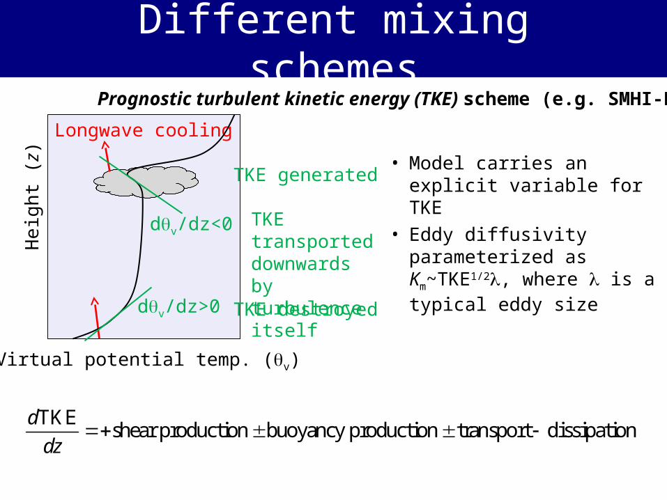
Longwave cooling
Different mixing schemes
• Model carries an explicit variable for TKE
• Eddy diffusivity parameterized as Km~TKE1/2, where is a typical eddy size
Virtual potential temp. (v)
Heig
ht (z
)
Prognostic turbulent kinetic energy (TKE) scheme (e.g. SMHI-RCA)
dv/dz<0
TKEshear production buoyancy production transport dissipation
d
dz
dv/dz>0
TKE generated
TKE destroyed
TKE transported downwards by turbulence itself

Observed Radar And Lidar
Figures from cloud-net.org

Cloud values compared
• Cloud Existence• Cloud Top• Cloud Base
• Cloud Thickness• Liquid Water Path
ObservedCloudFraction
ECMWFModelCloudFraction

Composite over diurnal cycle

Liquid Water Composite

Biases and random errors
Model Cloud Top
(m) Cloud Base
(m)
Cloud Thickness
(m)
Met Office Mesoscale -213 ± 370 -190 ± 307 -22 ± 429
Met Office Global -270 ± 416 -287 ± 365 +18 ± 485
ECMWF -126 ± 378 -84 ± 354 -42 ± 416
Météo France -567 ± 415 -326 ± 366 -241 ± 443
KNMI – RACMO 63 ± 432 -115 ± 357 178 ± 495
SMHI-RCA -46 ± 778 -387 ± 436 341 ± 823 Worst two models in terms of bias and random error
• Tendency for all models to place cloud too low

Conclusions
• Met Office Mes best at placing clouds at right time• Met Office, ECMWF & RACMO best diurnal cycle
– All use non-local mixing with explicit entrainment– Met Office and ECMWF clouds too low by 1 model level– RACMO height good: ECMWF physics but higher res.
• Meteo-France clouds too low and thin– Local mixing scheme underestimates growth
• SMHI-RCA clouds too thick and evolve little through the day– Only model to use prognostic turbulent kinetic energy