WORKING PAPER SERIES

Evaluating FOMC Forecasts

William T. Gavin and Rachel J. Mandal

Working Paper 2001-005Chttp://research.stlouisfed.org/wp/2001/2001-005.pdf

Revised August 2002

FEDERAL RESERVE BANK OF ST. LOUISResearch Division411 Locust Street

St. Louis, MO 63102

______________________________________________________________________________________

The views expressed are those of the individual authors and do not necessarily reflect official positions ofthe Federal Reserve Bank of St. Louis, the Federal Reserve System, or the Board of Governors.

Federal Reserve Bank of St. Louis Working Papers are preliminary materials circulated to stimulatediscussion and critical comment. References in publications to Federal Reserve Bank of St. Louis WorkingPapers (other than an acknowledgment that the writer has had access to unpublished material) should becleared with the author or authors.

Photo courtesy of The Gateway Arch, St. Louis, MO. www.gatewayarch.com

EVALUATING FOMC FORECASTS

Revised August 2002

Abstract

Monetary policy outcomes have improved since the early 1980s. One factor contributingto the improvement is that Federal Reserve policymakers began reporting economicforecasts to Congress in 1979. These forecasts indicate what the Federal Open MarketCommittee (FOMC) members think will be the likely consequence of their policies. Weevaluate the accuracy of the FOMC forecasts relative to private sector forecasts, theforecasts of the Research Staff at the Board of Governors, and a naïve alternative. Wefind that the FOMC output forecasts were better than the naïve model and at least as goodas those of the private sector and the Fed staff. The FOMC inflation forecasts were moreaccurate than the private sector forecasts and the naïve model; for the period ending in1996, however, they were not as accurate as Fed staff inflation forecasts.

KEYWORDS: Federal Reserve, Forecast Evaluation, Monetary Policy

JEL CLASSIFICATION: E37, E52

William T. Gavin Rachel J. MandalVice President and Economist Research AnalystResearch Department Research DepartmentFederal Reserve Bank of St. Louis Federal Reserve Bank of St. LouisP.O. Box 442 P.O. Box 442St. Louis, MO 63166 St. Louis, MO 63166Ph. (314) 444-8578 Ph. (314) 444-8520FAX (314) 444-8731 FAX (314) 444-8731gavin@stls.frb.org rachel.j.mandal@stls.frb.org

We thank Dean Croushore, Chris Neely, Jeremy Piger, Robert Rasche, Pierre Siklos, andtwo anonymous referees for helpful comments.

1

1. Introduction

For the 15 years leading up to 1979, U.S. inflation accelerated and became more

uncertain. Since 1979, inflation has declined dramatically and has become less volatile.

There was an institutional change in 1979 that contributed to the improved policy

environment. In that year the Fed began providing Congress with economic forecasts,

thus allowing some insight into policymakers’ beliefs and monetary policy intentions.

There has been an extensive analysis of the research staff forecasts, but not of the

FOMC forecasts.1 The FOMC forecasts that we evaluate are forecasts of the individual

policymakers, not the research staff. The Fed reports two summary statistics of the

individual forecasts. The first is the low and the high forecast among all the

policymakers. The second, which is referred to as the central tendency, omits extreme

forecasts; it is a smaller range that is meant to better represent the consensus view. In this

article, we define the FOMC forecast as the midpoint of the full range of the individual

forecasts. We do not report results for the central tendency because the full range

performed at least as well as the central tendency on every dimension we examined.2

We examine the accuracy and efficiency of the FOMC forecasts and compare

them with three alternative forecasts: a naïve “same change” forecast, the Blue Chip

consensus forecast (Blue Chip), and the Federal Reserve Research Staff forecast (Green

Book) that is prepared for FOMC meetings. After examining the rationality of the

FOMC forecasts, we compare them with the alternatives in tests of accuracy and

encompassing.

1 For recent studies of Fed staff forecasts, see Jansen and Kishan (1996), Joutz and Stekler (2000), andRomer and Romer (2000).2 Gavin and Mandal (2001) use the central tendency to show that the Blue Chip consensus may be a goodmonthly proxy for the unobserved expectations of policymakers.

2

2. The Data

This study examines forecasts for output growth and inflation. The forecast intervals

are measured as the fourth-quarter-over-fourth-quarter growth rate for 1979 through

2001. There are three forecast horizons from which the four-quarter growth rate is

predicted. The three forecasts are made early in the months of February and July,

approximately 18, 12, and 6 months before the actual data are released. We use this

convention to label the forecasts. That is, the forecasts made in July for the next year are

labeled 18-month, the forecasts made at the beginning of February are defined as 12-

month, and the July updates of the annual forecasts are called 6-month forecasts. In the

case of the July updates, the forecaster has information from the first six months of the

year, so they are actually predicting what will happen in the second half of the year.

To measure actual output and inflation, we use real-time data rather than the latest

vintage data. We use the real-time data for the full calendar year as they were first

reported at the end of January in the following year. We think it is appropriate to use

these real-time data for three reasons. First, financial market participants and

policymakers are most interested in how economic news affects asset prices; the primary

impact of an economic news release occurs with the first release of data. Second, we

assume that subsequent data revisions are random and our relative evaluation of the

forecasts would not change if we used later vintages of the data.3 Third, this vintage is

3 Zarnowitz and Braun (1993, Table 5) report forecast errors measured at various stages of revision and findlittle difference in the errors as GDP data are revised. Schuh (2001) uses current vintage data in anevaluation of private-sector forecasts. He reports that measures of relative accuracy do not change muchwhen he uses real-time data. Faust, Rogers, and Wright (2000) study GNP/GDP revisions in the G-7 andfind mixed evidence that revisions are random. The revisions appear to be so for the United States, but notfor all the G-7 countries. McNees (1988) argues for using the latest vintage of data but reports in his Table4 that the measure of forecast accuracy does not seem to depend much on which vintage of data is used.

3

the one the FOMC observed before making policy at the first FOMC meeting of each

year. If one wants to study policy reaction functions, then one should use the real-time

data that policymakers had available when they were making policy and preparing

forecasts for the year ahead.4

2.1 The FOMC forecast

Since July 1979, the FOMC has made forecasts of growth rates for nominal GDP,

real GDP, and inflation.5 There is a complication in evaluating the FOMC inflation

forecasts because the FOMC switched among price indexes over our sample period. The

FOMC began forecasting the implicit price deflator for GNP in 1979 and continued

reporting forecasts for the deflator until 1989, when it began making inflation forecasts in

terms of the consumer price index (CPI). In 2000, the FOMC switched once again, this

time to the chain price index for personal consumption expenditures (PCE). We begin by

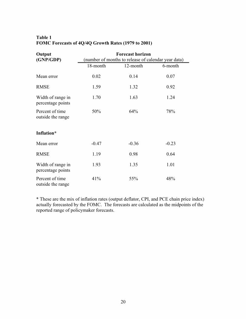
looking at the forecasts that were made for the different indexes (Figure 1 and Table 1).

However, in the statistical evaluation of the forecasting record, we use an implied

forecast that is calculated by subtracting the midpoint of the range of real output forecasts

from the midpoint of the range of nominal output forecasts (Tables 2 through 6). We do

this because the FOMC has consistently forecasted nominal and real output throughout

the entire period.

2.2 The naïve forecast

4 Croushore and Evans (2000) use a structural VAR method to show that estimated monetary policy shocksare quite similar regardless of whether one is using current vintage or real-time data.5 The government switched from GNP to GDP in 1992.

4

The first alternative is a naïve model. The naïve model predicts that the future

growth rate will be the same as the most recently observed growth rate. The definition

makes sense in the case where the forecasted variables have a growth trend. It also

makes more sense when using four-quarter rather than quarterly data, which tend to be

volatile with offsetting variation within the year.

2.3 The Blue Chip consensus forecast

Our second alternative is the consensus forecast of the business economists who

participate in the Blue Chip Economic Indicators survey. We use the Blue Chip

consensus forecast because we think the Blue Chip forecast is representative of the best

private sector forecasts. The Blue Chip began compiling and reporting forecasts at about

the same time the FOMC began reporting forecasts to Congress. The Blue Chip

consensus forecasts used in this study are taken from the February and July reports. The

Blue Chip consensus forecasts the same variables over the same horizon and in

approximately the same time frame as the FOMC forecasts.

Schuh (2001) evaluates the year-ahead forecasts of three private sources of

economic forecasts: the Survey of Professional Forecasters, forecasters surveyed by the

Wall Street Journal, and the Blue Chip consensus. He shows that the forecast errors from

each of these three sources look quite similar. A visual inspection of the plotted errors

for output and inflation reveals that, although the forecasts appear to be very similar, the

Blue Chip output forecast looks best in the periods when the output forecast errors were

large (in the early 1980s and in the late 1990s). We use the consensus forecast from the

5

Blue Chip because it is better than the individual forecasts and because we are using a

consensus forecast from the policymakers.6

2.4 The Green Book forecast

The third alternative we examine is the Green Book forecast produced by the

research staff at the Board of Governors of the Federal Reserve System. FOMC

members had access to the Green Book forecasting process continuously throughout the

year, and no doubt the FOMC forecasts could have been influenced by information

provided by this process. We should note that FOMC members submit their forecasts

before they see the Green Book. However, they have an opportunity to revise their

forecasts after the FOMC meets and decides on policy. Therefore, it is possible that

information in the Green Book may be reflected in the final FOMC member forecasts.

The series on Green Book forecasts ends in 1996 because these forecasts are not available

to the public until at least five years after the meeting for which they are prepared.

3. Is the FOMC forecast unbiased and efficient?

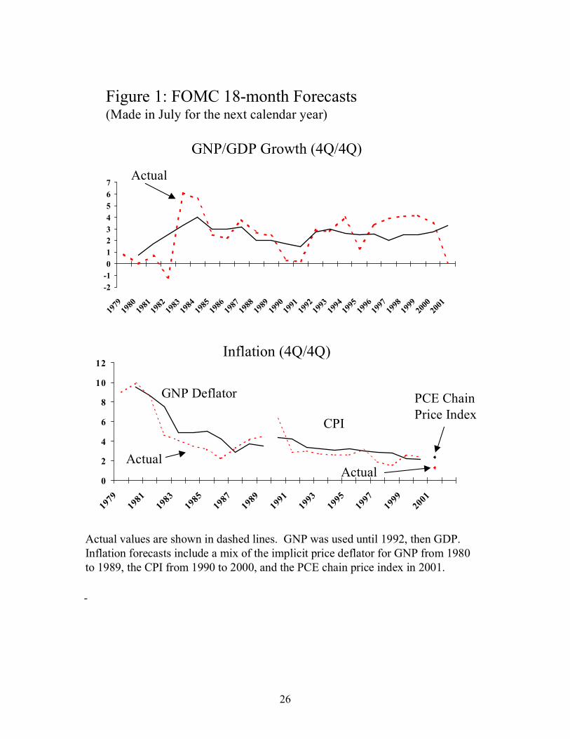
Figure 1 shows the 18-month FOMC forecasts for output growth and inflation, as

well as the actual values. Economic forecasters are notoriously bad at predicting turning

points. The FOMC members are no exception. Generally, they missed the large decline

of inflation that occurred during 1981 to 1986 and the recessions in output in 1980-1982,

1990-1991, and 2001.7 Table 1 reports summary statistics for the FOMC forecasts,

6 McNees (1987) and Batchelor and Dua (1991) evaluate the relationship between the Blue Chip

consensus and the individual forecasts.7 Joutz and Stekler (2000) show that both the Fed staff and private forecasters missed business cycleturning points in GNP growth and failed to predict the large decline in inflation in the early 1980s.

6

including the mean error, the root-mean-squared error (RMSE), the average distance in

percentage points between the high and low forecast, and, finally, the percentage of times

that the actual value fell outside the range of FOMC forecasts. The RMSE is a measure

of the predictive uncertainty faced by the forecaster. The width of the range measures the

dispersion in the individual forecasts and it can be considered a measure of the consensus

among the individual policymakers.

The RMSEs of the policymakers’ forecasts are much smaller than those

calculated from forecasts in earlier sample periods. Part of this reflects a well-known

decline in volatility in the U.S. economy that began in the mid-1980s.8 Joutz and Stekler

(2000) report a substantial reduction in the variance of inflation and output growth in the

second half of the 1980s. In their Table 4 they report the RMSE for Fed staff forecasts of

four-quarter spans between 1965 and 1989. The RMSEs for output growth (2.42) and

inflation (1.83) forecasts made early in the quarter are almost twice as large as those

observed in the period from 1980 through 2001. The RMSE for the FOMC’s output

growth forecasts made early in February was 1.32; for inflation it was 0.98.

The mean errors for the output forecasts are close to zero for all forecast horizons,

but the mean errors for the inflation forecasts show that the FOMC tended to over-predict

the inflation rate. This apparent bias gets smaller as the forecast horizon shrinks. As one

might expect, both the RMSEs and the dispersion of the individual forecasts decline as

the forecast horizon becomes shorter.

Is the width of the range of individual point forecasts a good measure of the

predictive uncertainty faced by an individual forecaster? Zarnowitz and Lambros (1987)

8 McNees (1992) shows that perhaps the most crucial determinant of the size of a forecast error is theparticular sample period for which the forecast is made.

7

use data from the ASA-NBER survey of professional forecasters to show that, while

these measures of consensus are correlated with measures of predictive uncertainty, the

measures of consensus tend to understate the amount of predictive uncertainty. This

result is also evident in our data. In every case, the midpoint plus and minus one RMSE

is larger than the range of forecasts.

In the case of the output forecasts, the actual growth rate fell outside the range

more than 50 percent of the time for all three forecast horizons. It is interesting that as

the forecast horizon becomes shorter, the degree of consensus seems to increase faster

than the underlying uncertainty falls. This result reflects both a relatively large amount

of predictive uncertainty about real output growth and a relatively large degree of

consensus about how to interpret incoming economic data. The point estimates converge

faster than the predictive uncertainty declines such that the actual output growth rate is

less likely to fall within the forecast range as the forecast horizon becomes shorter.

Although the forecasts of inflation appear to be biased, the predictive uncertainty

for inflation is less than that for output growth at all forecast horizons. Öller and Barot

(2000) note a similar result for output and inflation forecasts from a group of 13

European economies. Despite the lower amount of predictive uncertainty about inflation,

the FOMC members seem to have a harder time agreeing on a point forecast for inflation

when the forecast horizon is greater than a year ahead. Note that for the 6- and 12-month

forecasts, the policymakers are better able to come to a consensus on inflation than they

are on output. One hypothesis for this anomaly is that at shorter horizons the

policymakers believe that inflation is essentially “baked into the cake.” They don’t

believe that anything they do with policy will have much impact on inflation within the

8

next year. However, the 18-month forecast is far enough away that their inflation

forecast will reflect to a greater degree their beliefs about the medium-term objective.

3.1 Is the FOMC forecast unbiased?

In this section, we check the alternative forecasts for bias. We estimate the

following regression in the first part of our test:

x xt t i tf

t i t= + +− −α β ε , (1)

where x is the variable being forecast (the fourth-quarter-over-fourth-quarter growth rate

of output or the price deflator for output). The forecast (xf) is indexed by the time when

the forecast was made (t-i, where i refers to three forecast horizons) and the year to which

it applies (t). If the estimates of (a, b) are equal to (0, 1), the forecasts are unbiased. We

use an F-statistic to test for unbiasedness. Holden and Peel (1990) show that even if we

can reject the null hypothesis that (a, b) is equal to (0, 1), it is still possible that the

forecasts may be unbiased. The intuition for their result can be understood by thinking

about equation (1) as a mechanism for combining unbiased forecasts where the constant

is an unbiased forecast of the series. If we cannot reject the null hypothesis, we can

conclude that the forecast is unbiased. If we reject the null hypothesis, it is necessary to

examine the properties of the forecast error, .ft t i tx x−− To make a complete test of bias,

we also compute the regression

ft t i t t i tx x γγ ε− −− = + (2)

and test whether γ is equal to zero. In addition, we must take account of possible serial

correlation in the error for the 18-month forecast. Because the forecast horizon is longer

than the interval over which output growth is measured, the forecast error for year t is not

9

available when the forecasts for year t+1 are made. Therefore, information that arrives in

the second half of year t may be reflected in forecast errors for both years t and t+1. If it

is, the errors will display first-order serial correlation. For this case, Hansen (1982) has

shown that ordinary least squares (OLS) estimates will be unbiased, but the standard

errors will be too small, leading to too many rejections of the null hypothesis. Therefore

we used the correction for serial correlation suggested by Hansen (1982) when reporting

test statistics for the July next-year forecasts.

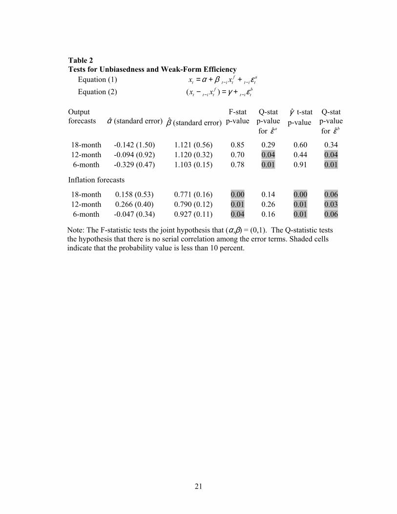
OLS estimates of equations (1) and (2) for the output and inflation forecasts are

listed in Table 2. Table 2 includes the estimates of α and β, with standard errors in

parentheses. The third column of results shows the probability values of the F-statistic

for the null joint hypothesis that (a, b) = (0, 1). For the three cases with output, the

probability values are all above 50 percent, so we conclude that the output forecasts are

unbiased. It is not necessary to estimate equation (2) in the case of the output forecasts,

however, because we could not reject that the forecasts are unbiased using the F-statistic.

In contrast, the probability values of the F-statistic for the inflation forecasts are quite

low, always less than 10 percent. To complete the test for bias, the fifth column of Table

2 reports the probability values for the t-statistic for testing whether γ̂ is equal to zero.

Here we find strong evidence that the FOMC inflation forecasts are biased.

These results contrast with past studies of inflation forecasts where the evidence

bias is mixed. For example, neither Romer and Romer (2000) nor Joutz and Stekler

(2000) can reject the null joint hypothesis that (a, b) = (0, 1) for the Green Book inflation

forecasts, even at a forecast horizon of 1 year. However, Romer and Romer reject the

10

null joint hypothesis for the Blue Chip inflation forecasts in the period from 1980 to

1991.

-

3.2 Is the FOMC forecast efficient?

If the FOMC forecasts are efficient, they will take account of information in the

most recent output and inflation data as well as what they have learned from previous

forecast errors. A weak form test for informational efficiency is a test for serial

correlation in the forecast errors. The fourth and sixth columns of Table 2 include Q-

statistics that are used to test whether the estimated errors are random. In general, these

Q-statistics indicate that there is serial correlation in estimated residuals from equations

(1) and (2), except in the case of the 18-month output forecast. Joutz and Stekler (2000)

reported that although the Fed staff’s four-quarter-ahead inflation forecasts were unbiased

in the earlier period, they found significant serial correlation in the forecast error.

We also test for informational efficiency by checking to see if the forecast errors

are orthogonal to the previous year’s output and inflation data and the past forecast errors

that were revealed when that data became available. All forecasters can observe last

year's errors just before they make their current-year forecasts in February and July.

Thus, the current year’s forecast errors should not be correlated with any of the previous

year's forecast errors. As noted above, the 18-month forecast overlaps with the current-

year forecasts. Therefore, even if the forecasts are efficient, the errors in the previous

year's forecasts may be correlated with the errors in the 18-month forecast. If the

forecasts are efficient, the forecast errors from two years ago should not be correlated

with these forecast errors.

11

Most forecasters believe that inflation and output are related and that past errors

in both these measures should be taken into account when forecasting either inflation or

output. Thus, we also check to see whether past inflation forecast errors are correlated

with current output forecast errors (and vice versa).

To conduct these orthogonality tests for efficiency, we run the following

regression:

t i t t i t jk

t i te e u- - - -= + +a b , (3)

where t i te- is the forecast error for year t (for either output or inflation) made at the t-i

horizon. Because the data set is small, we check for bivariate relationships between the

current and past errors. There will be a total of six different dependent variables: three

for output and three for inflation from each of the forecast horizons. The term t i t jke- - is

the error in the forecast for year t-j made at the t-i forecast horizon. The superscript k

refers to an error from either the inflation or the output forecast. In principle, we could

test efficiency against any information that was available at the time the forecasts were

made. Here we are checking against the most recent errors for inflation and output that

were known. Thus, j = 2 when the dependent variable is a July next-year forecast error,

and j = 1 when it is a current-year forecast error. We also test efficiency against

information about the most recent information available on inflation and output by

replacing the error term, ,kt i t je− − with the actual values for output growth and inflation.

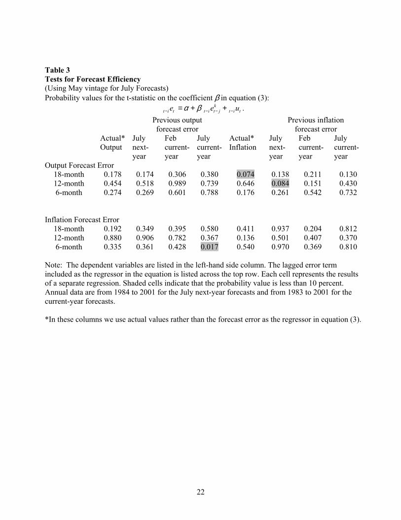
Estimation results for equation (3) are shown in Table 3. The table includes the

p-values for the t-statistic testing the null hypothesis that b = 0. Each p-value is

calculated in a separate regression. The only statistically significant correlations are with

forecast errors from a different variable. Of the 48 cases we examined, we could reject

12

orthogonality in only three. Two cases involved output forecast errors. The 18-month

output error was related to the actual inflation rate from two years ago and the 12-month

output error was correlated with the previous 18-month inflation forecast error. The other

significant relationship was between the 6-month inflation forecast error and the previous

year’s 6-month output forecast error.

4. How does the FOMC perform relative to alternative forecasts?

4.1 Is the FOMC forecast as accurate as the alternatives?

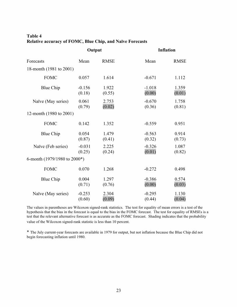
We begin by comparing the FOMC forecasts with the Blue Chip and naïve

forecasts for the period from 1979 to 2001. Table 4 reports the mean error, the RMSE,

and the probability value for a two-sided Wilcoxon signed-rank test that evaluates the

significance of the difference in the size of the forecast errors. Diebold and Mariano

(1995) show that the Wilcoxon signed-rank test statistic is well-sized in cases where the

sample is small and the alternative forecast errors are highly correlated (and possibly

serially correlated—as we expect for the 18-month forecasts). In tests of whether the

RMSEs are equal, we assume that the forecasters’ loss function is measured by the square

of the forecast error. However, there was a substantial bias in inflation forecasts and we

want to test whether the differences in bias among the forecasts is statistically significant;

therefore, we also construct a test of the mean error in which we measure the forecaster’s

loss function as the forecast error.

The mean errors for the output forecasts are shown in the first column in Table 4.

There were no significant differences between the bias in the FOMC output forecasts and

the others. The FOMC output forecast had lower RMSEs than either the Blue Chip or

13

the naïve forecast at all three forecast horizons. However, the FOMC output forecast was

not significantly more accurate than the Blue Chip forecast. The FOMC’s output forecast

was significantly better than the naïve forecast for both the 18- and 6-month horizons.

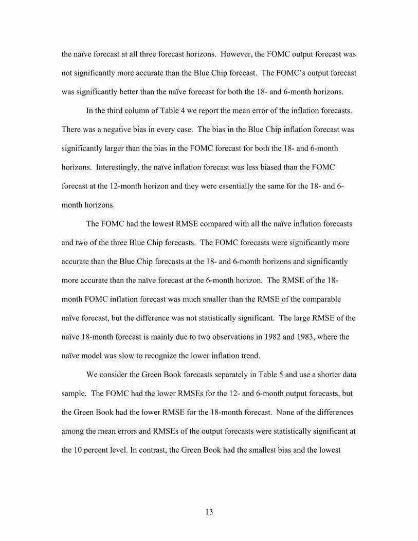
In the third column of Table 4 we report the mean error of the inflation forecasts.

There was a negative bias in every case. The bias in the Blue Chip inflation forecast was

significantly larger than the bias in the FOMC forecast for both the 18- and 6-month

horizons. Interestingly, the naïve inflation forecast was less biased than the FOMC

forecast at the 12-month horizon and they were essentially the same for the 18- and 6-

month horizons.

The FOMC had the lowest RMSE compared with all the naïve inflation forecasts

and two of the three Blue Chip forecasts. The FOMC forecasts were significantly more

accurate than the Blue Chip forecasts at the 18- and 6-month horizons and significantly

more accurate than the naïve forecast at the 6-month horizon. The RMSE of the 18-

month FOMC inflation forecast was much smaller than the RMSE of the comparable

naïve forecast, but the difference was not statistically significant. The large RMSE of the

naïve 18-month forecast is mainly due to two observations in 1982 and 1983, where the

naïve model was slow to recognize the lower inflation trend.

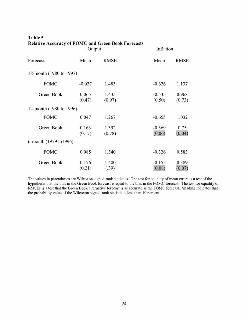
We consider the Green Book forecasts separately in Table 5 and use a shorter data

sample. The FOMC had the lower RMSEs for the 12- and 6-month output forecasts, but

the Green Book had the lower RMSE for the 18-month forecast. None of the differences

among the mean errors and RMSEs of the output forecasts were statistically significant at

the 10 percent level. In contrast, the Green Book had the smallest bias and the lowest

14

RMSE for all the inflation forecasts. The differences were significant for the 12- and 6-

month forecasts.

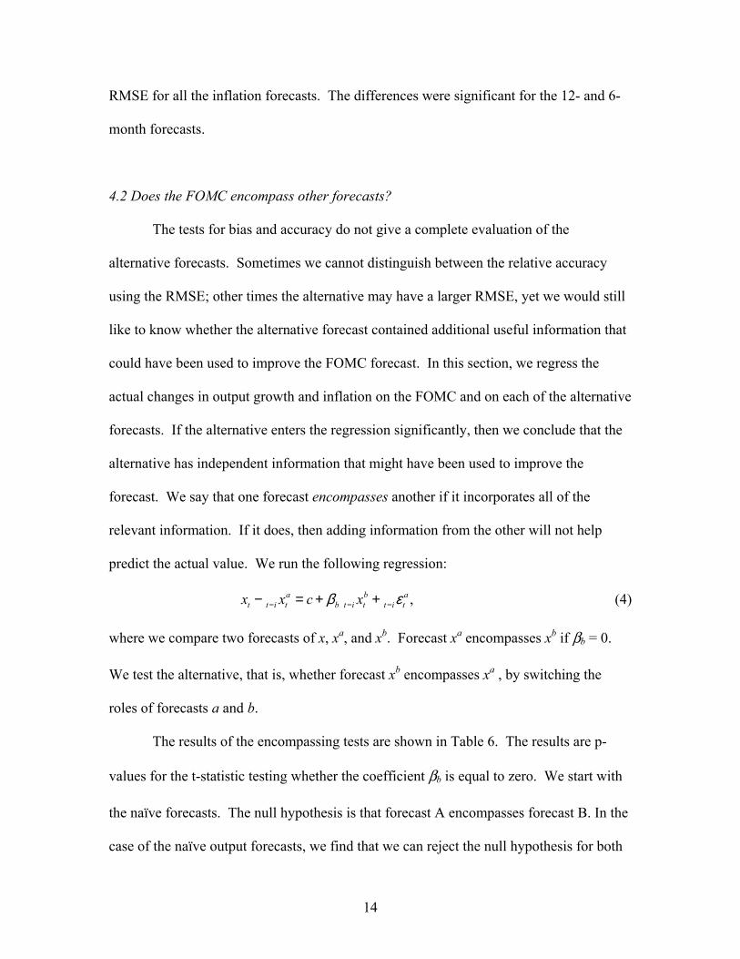
4.2 Does the FOMC encompass other forecasts?

The tests for bias and accuracy do not give a complete evaluation of the

alternative forecasts. Sometimes we cannot distinguish between the relative accuracy

using the RMSE; other times the alternative may have a larger RMSE, yet we would still

like to know whether the alternative forecast contained additional useful information that

could have been used to improve the FOMC forecast. In this section, we regress the

actual changes in output growth and inflation on the FOMC and on each of the alternative

forecasts. If the alternative enters the regression significantly, then we conclude that the

alternative has independent information that might have been used to improve the

forecast. We say that one forecast encompasses another if it incorporates all of the

relevant information. If it does, then adding information from the other will not help

predict the actual value. We run the following regression:

,a b at t i t b t i t t i tx x c xβ ε− − −− = + + (4)

where we compare two forecasts of x, xa, and xb. Forecast xa encompasses xb if bb = 0.

We test the alternative, that is, whether forecast xb encompasses xa , by switching the

roles of forecasts a and b.

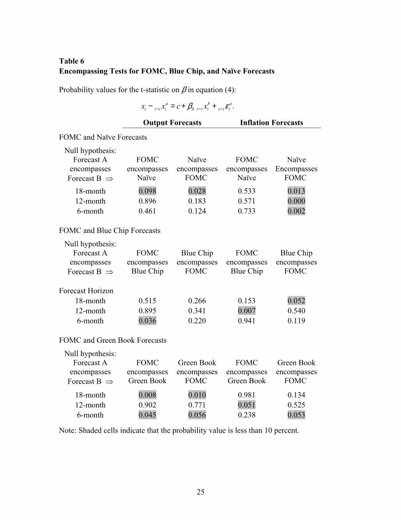
The results of the encompassing tests are shown in Table 6. The results are p-

values for the t-statistic testing whether the coefficient bb is equal to zero. We start with

the naïve forecasts. The null hypothesis is that forecast A encompasses forecast B. In the

case of the naïve output forecasts, we find that we can reject the null hypothesis for both

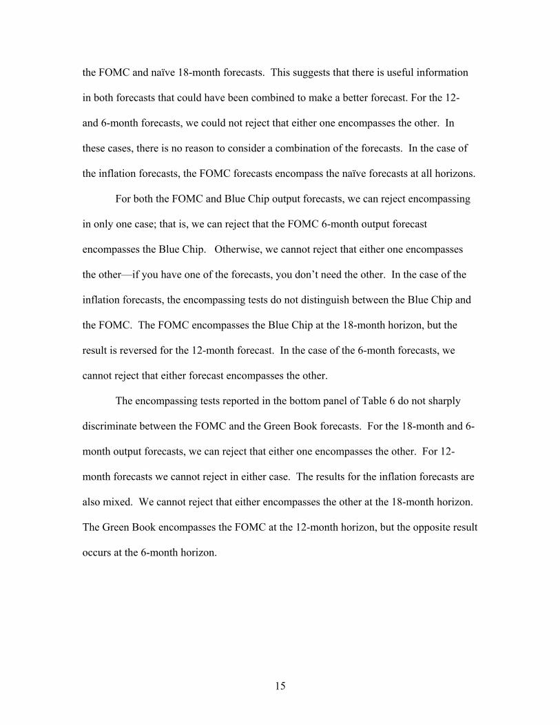
15

the FOMC and naïve 18-month forecasts. This suggests that there is useful information

in both forecasts that could have been combined to make a better forecast. For the 12-

and 6-month forecasts, we could not reject that either one encompasses the other. In

these cases, there is no reason to consider a combination of the forecasts. In the case of

the inflation forecasts, the FOMC forecasts encompass the naïve forecasts at all horizons.

For both the FOMC and Blue Chip output forecasts, we can reject encompassing

in only one case; that is, we can reject that the FOMC 6-month output forecast

encompasses the Blue Chip. Otherwise, we cannot reject that either one encompasses

the other—if you have one of the forecasts, you don’t need the other. In the case of the

inflation forecasts, the encompassing tests do not distinguish between the Blue Chip and

the FOMC. The FOMC encompasses the Blue Chip at the 18-month horizon, but the

result is reversed for the 12-month forecast. In the case of the 6-month forecasts, we

cannot reject that either forecast encompasses the other.

The encompassing tests reported in the bottom panel of Table 6 do not sharply

discriminate between the FOMC and the Green Book forecasts. For the 18-month and 6-

month output forecasts, we can reject that either one encompasses the other. For 12-

month forecasts we cannot reject in either case. The results for the inflation forecasts are

also mixed. We cannot reject that either encompasses the other at the 18-month horizon.

The Green Book encompasses the FOMC at the 12-month horizon, but the opposite result

occurs at the 6-month horizon.

16

5. Conclusions

This study examines the forecasts of Federal Reserve policymakers. While many

have studied the forecasts of the Federal Reserve staff (the Green Book forecasts), this is

the first in-depth statistical analysis of the forecasts made by the policymakers

themselves. The forecasts are reported as a range of individual forecasts, which may be

thought of as a measure of consensus among the policymakers. Forecasts are made at

18-, 12-, and 6-month horizons. As one would expect, both the degree of consensus and

the predictive uncertainty fall as the horizon becomes shorter, although the consensus

converges faster than the predictive uncertainty declines. Generally, the outcome is more

likely to fall outside the full range of forecasts as the horizon becomes shorter.

In testing for bias and informational efficiency in the FOMC forecasts, we find

that the long-term output forecast was unbiased and displayed a weak form of

informational efficiency. There is some evidence of serial correlation among the errors

for the shorter-term output forecast. The inflation forecasts are biased and the errors are

serially correlated. For the most part, we find that the forecast errors for both inflation

and output pass tests for orthogonality with the previous forecast errors and the most

recently observed values of output growth and inflation. There is some evidence that the

FOMC did not make efficient use of the dynamic relationship between inflation and

output.

In comparisons with alternative forecasts, we find that the FOMC output forecast

is more accurate than the naïve model and as accurate as the private sector Blue Chip and

the Fed staff’s Green Book forecast. The FOMC forecasts look like those from the

private sector and the Fed staff, sometimes better and sometimes worse. The FOMC

17

output forecast often had the lowest RMSE. Yet, even in some of those cases, the

encompassing results show that there was information in alternative forecasts that might

have been used to improve the FOMC forecasts.

The results of the inflation forecasts are interesting. On average, inflation fell

throughout the sample period and all of the forecasts tended to overestimate inflation.

The bias in the inflation forecasts is larger at longer horizons, but is statistically

significant even for forecasts made when the year was half over. The FOMC inflation

forecasts are more accurate than the Blue Chip, but not as accurate as the Green Book.

Thus, our results support the main result in Romer and Romer (2000). They concluded

that policymakers had access to inside information about the inflation outlook because

the Green Book inflation forecasts were significantly better than the private sector

forecasts. The policymakers were aware of the staff forecasts, and our results are

consistent with the idea that the FOMC members took some account of this information

when making their own forecasts.

18

References

Batchelor, R., & Dua, P. (1991). Blue Chip rationality tests. Journal of Money, Creditand Banking 23, 692-705.

Croushore, D., & Evans, C. L. (2000). Data revisions and the identification of monetarypolicy shocks, Federal Reserve Bank of Chicago, Working Paper WP-00-26.

Diebold, F. X., & Mariano, R. S. (1995). Comparing predictive accuracy. Journal ofBusiness and Economic Statistics 13, 253-263.

Faust, J., Rogers, J. H., & Wright, J.H. (2000). News and noise in G-7 GDPannouncements. Board of Governors of the Federal Reserve System, InternationalFinance Discussion Papers 690.

Gavin, W. T., & Mandal, R.J. (2001). Forecasting inflation and growth: Do privateforecasts match those of policymakers? Business Economics January, 13-20.

Hansen, L. P. (1982). Large sample properties of generalized method of momentsestimators. Econometrica 50, 1029-54.

Holden, K.& Peel, D.A. (1990). On testing for unbiasedness and efficiency of forecasts.The Manchester School 58, 120-127.

Jansen, D. W., & Kishan, R. P. (1996). An evaluation of Federal Reserve forecasting.Journal of Macroeconomics 18, 89-100.

Joutz, F., & Stekler, H.O. (2000). An evaluation of the predictions of the FederalReserve. International Journal of Forecasting 16, 17-38.

McNees, S. K. (1992). How large are economic forecast errors? New England EconomicReview July/August, 25-42.

________. (1988). How accurate are macroeconomic forecasts?” New EnglandEconomic Review July/August, 15-36.

________. (1987). Consensus forecasts: tyranny of the majority?” New EnglandEconomic Review November/December, 15-21.

Öller, L. & Barot, B. (2000). The accuracy of European growth and inflation forecasts.International Journal of Forecasting 16, 293-315.

Romer, C. D. & Romer D. H. (2000). Federal Reserve private information and thebehavior of interest rates. American Economic Review 90, 429-57.

19

Schuh, S. (2001). An evaluation of recent macroeconomic forecast errors. New EnglandEconomic Review January/February, 35-56.

Zarnowitz, V., & Braun, P. (1993). Twenty-two years of the NBER-ASA QuarterlyEconomic Outlook Surveys: Aspects and comparisons of forecastingperformance. Business Cycles, Indicators, and Forecasting, Stock, J. H. &Watson, M. W., eds., The University of Chicago Press, Chicago, 11-84.

Zarnowitz, V. & Lambros, L. A. (1987). Consensus and uncertainty in economicprediction. Journal of Political Economy 95, 591-621.

20

Table 1 FOMC Forecasts of 4Q/4Q Growth Rates (1979 to 2001)

Output(GNP/GDP)

Forecast horizon(number of months to release of calendar year data)

18-month 12-month 6-month

Mean error 0.02 0.14 0.07

RMSE 1.59 1.32 0.92

Width of range inpercentage points

1.70 1.63 1.24

Percent of timeoutside the range

50% 64% 78%

Inflation*

Mean error -0.47 -0.36 -0.23

RMSE 1.19 0.98 0.64

Width of range inpercentage points

1.93 1.35 1.01

Percent of timeoutside the range

41% 55% 48%

* These are the mix of inflation rates (output deflator, CPI, and PCE chain price index)actually forecasted by the FOMC. The forecasts are calculated as the midpoints of thereported range of policymaker forecasts.

21

Table 2 Tests for Unbiasedness and Weak-Form Efficiency Equation (1) f a

t t i t t i tx xα β ε− −= + + Equation (2) ( )f b

t t i t t i tx x γ ε− −− = +

Outputforecasts α̂ (standard error) β̂ (standard error)

F-statp-value

Q-statp-valuefor ˆaε

γ̂ t-statp-value

Q-statp-valuefor ˆbε

18-month -0.142 (1.50) 1.121 (0.56) 0.85 0.29 0.60 0.3412-month -0.094 (0.92) 1.120 (0.32) 0.70 0.04 0.44 0.046-month -0.329 (0.47) 1.103 (0.15) 0.78 0.01 0.91 0.01

Inflation forecasts

18-month 0.158 (0.53) 0.771 (0.16) 0.00 0.14 0.00 0.0612-month 0.266 (0.40) 0.790 (0.12) 0.01 0.26 0.01 0.036-month -0.047 (0.34) 0.927 (0.11) 0.04 0.16 0.01 0.06

Note: The F-statistic tests the joint hypothesis that (α,β) = (0,1). The Q-statistic teststhe hypothesis that there is no serial correlation among the error terms. Shaded cellsindicate that the probability value is less than 10 percent.

22

Table 3Tests for Forecast Efficiency (Using May vintage for July Forecasts)Probability values for the t-statistic on the coefficient β in equation (3):

.kt i t t i t j t i te e uα β− − − −= + +

Previous outputforecast error

Previous inflationforecast error

Actual*Output

Julynext-year

Febcurrent-year

Julycurrent-year

Actual*Inflation

Julynext-year

Febcurrent-year

Julycurrent-year

Output Forecast Error18-month 0.178 0.174 0.306 0.380 0.074 0.138 0.211 0.13012-month 0.454 0.518 0.989 0.739 0.646 0.084 0.151 0.4306-month 0.274 0.269 0.601 0.788 0.176 0.261 0.542 0.732

Inflation Forecast Error18-month 0.192 0.349 0.395 0.580 0.411 0.937 0.204 0.81212-month 0.880 0.906 0.782 0.367 0.136 0.501 0.407 0.3706-month 0.335 0.361 0.428 0.017 0.540 0.970 0.369 0.810

Note: The dependent variables are listed in the left-hand side column. The lagged error termincluded as the regressor in the equation is listed across the top row. Each cell represents the resultsof a separate regression. Shaded cells indicate that the probability value is less than 10 percent.Annual data are from 1984 to 2001 for the July next-year forecasts and from 1983 to 2001 for thecurrent-year forecasts.

*In these columns we use actual values rather than the forecast error as the regressor in equation (3).

23

Table 4 Relative accuracy of FOMC, Blue Chip, and Naïve Forecasts

Output Inflation

Forecasts Mean RMSE Mean RMSE

18-month (1981 to 2001)

FOMC 0.057 1.614 -0.671 1.112

Blue Chip -0.156(0.18)

1.922(0.55)

-1.018(0.00)

1.359(0.01)

Naïve (May series) 0.061(0.79)

2.753(0.02)

-0.670(0.36)

1.758(0.81)

12-month (1980 to 2001)

FOMC 0.142 1.352 -0.559 0.951

Blue Chip 0.054(0.87)

1.479(0.41)

-0.563(0.32)

0.914(0.73)

Naïve (Feb series) -0.031(0.25)

2.225(0.24)

-0.326(0.01)

1.087(0.82)

6-month (1979/1980 to 2000*)

FOMC 0.070 1.268 -0.272 0.498

Blue Chip 0.004(0.71)

1.297(0.76)

-0.386(0.00)

0.574(0.03)

Naïve (May series) -0.253(0.60)

2.304(0.09)

-0.295(0.44)

1.130(0.04)

The values in parentheses are Wilcoxon signed-rank statistics. The test for equality of mean errors is a test of thehypothesis that the bias in the forecast is equal to the bias in the FOMC forecast. The test for equality of RMSEs is atest that the relevant alternative forecast is as accurate as the FOMC forecast. Shading indicates that the probabilityvalue of the Wilcoxon signed-rank statistic is less than 10 percent.

* The July current-year forecasts are available in 1979 for output, but not inflation because the Blue Chip did notbegin forecasting inflation until 1980.

24

Table 5 Relative Accuracy of FOMC and Green Book Forecasts

Output Inflation

Forecasts Mean RMSE Mean RMSE

18-month (1980 to 1997)

FOMC -0.027 1.483 -0.626 1.137

Green Book 0.065(0.47)

1.435(0.97)

-0.535(0.50)

0.968(0.73)

12-month (1980 to 1996)

FOMC 0.047 1.267 -0.655 1.032

Green Book 0.163(0.17)

1.392(0.78)

-0.369(0.06)

0.75(0.04)

6-month (1979 to1996)

FOMC 0.085 1.340 -0.326 0.583

Green Book 0.176(0.21)

1.400(.39)

-0.155(0.08)

0.389(0.07)

The values in parentheses are Wilcoxon signed-rank statistics. The test for equality of mean errors is a test of thehypothesis that the bias in the Green Book forecast is equal to the bias in the FOMC forecast. The test for equality ofRMSEs is a test that the Green Book alternative forecast is as accurate as the FOMC forecast. Shading indicates thatthe probability value of the Wilcoxon signed-rank statistic is less than 10 percent.

25

Table 6Encompassing Tests for FOMC, Blue Chip, and Naïve Forecasts

Probability values for the t-statistic on β in equation (4):

.a b at t i t b t i t t i tx x c xβ ε− − −− = + +

Output Forecasts Inflation Forecasts

FOMC and Naïve Forecasts

Null hypothesis:Forecast A

encompassesForecast B ⇒

FOMCencompasses

Naïve

Naïve

encompassesFOMC

FOMCencompasses

Naïve

Naïve

EncompassesFOMC

18-month 0.098 0.028 0.533 0.01312-month 0.896 0.183 0.571 0.0006-month 0.461 0.124 0.733 0.002

FOMC and Blue Chip Forecasts

Null hypothesis:Forecast A

encompassesForecast B ⇒

FOMCencompasses

Blue Chip

Blue Chip

encompassesFOMC

FOMCencompasses

Blue Chip

Blue Chip

encompassesFOMC

Forecast Horizon18-month 0.515 0.266 0.153 0.05212-month 0.895 0.341 0.007 0.5406-month 0.036 0.220 0.941 0.119

FOMC and Green Book Forecasts

Null hypothesis:Forecast A

encompassesForecast B ⇒

FOMCencompassesGreen Book

Green Bookencompasses

FOMC

FOMCencompassesGreen Book

Green Bookencompasses

FOMC

18-month 0.008 0.010 0.981 0.13412-month 0.902 0.771 0.051 0.5256-month 0.045 0.056 0.238 0.053

Note: Shaded cells indicate that the probability value is less than 10 percent.

26

-

-2-101234567

1979

1980

1981

1982

1983

1984

1985

1986

1987

1988

1989

1990

1991

1992

1993

1994

1995

1996

1997

1998

1999

2000

2001

Figure 1: FOMC 18-month Forecasts(Made in July for the next calendar year)

GNP/GDP Growth (4Q/4Q)

Actual

Inflation (4Q/4Q)

0

2

4

6

8

10

12

19791981

19831985

19871989

19911993

19951997

19992001

GNP Deflator

CPI

PCE ChainPrice Index

Actual values are shown in dashed lines. GNP was used until 1992, then GDP.Inflation forecasts include a mix of the implicit price deflator for GNP from 1980to 1989, the CPI from 1990 to 2000, and the PCE chain price index in 2001.

ActualActual