Embed Size (px)
Citation preview

Evaluating fish diet analysis methods byindividual-based modelling
Ida Ahlbeck, Sture Hansson, and Olle Hjerne
Abstract: Knowledge of diet compositions is important in ecological research. There are many methods available and nu-merous aspects of diet composition. Here we used modelling to evaluate how well different diet analysis methods describethe “true” diet of fish, expressed in mass percentages. The methods studied were both basic methods (frequency of occur-rence, dominance, numeric, mass, points) and composite indices (Index of Relative Importance, Comparative Feeding In-dex). Analyses were based on both averaged stomach content of individual fish and on pooled content from several fish.Prey preference, prey size, and evacuation rate influenced the performance of the diet analysis methods. The basic methodsperformed better than composite indices. Mass and points methods produced diet compositions most similar to the true dietand were also most robust, indicating that these methods should be used to describe energetic–nutritional sources of fish.
Résumé : Il importe de connaître la composition du régime alimentaire en recherche en écologie. De nombreuses méthodessont disponibles pour déterminer la composition du régime alimentaire, qui comporte de nombreux aspects. Nous avons uti-lisé la modélisation pour évaluer comment différentes méthodes d’analyse du régime alimentaire décrivent l’alimentation« réelle » des poissons, exprimée en terme de pourcentages de la masse. Les méthodes étudiées reposent tant sur des para-mètres de base (fréquence de l’occurrence, dominance, numérique, masse, points) que des indices composites (indice d’im-portance relative, indice comparatif d’alimentation). Les analyses sont basées sur le contenant stomacal moyen d’individuset sur le contenu stomacal combiné de plusieurs poissons. La performance des méthodes d’analyse de l’alimentation est in-fluencée par les préférences des proies, la taille des proies et le taux d’élimination. La performance des méthodes reposantsur des paramètres de base s’avère supérieure à celle de méthodes faisant appel à des indices composites. Les méthodes re-posant sur la masse et les points produisent les compositions du régime alimentaire qui s’approchent le plus du régime réelet sont également les plus robustes. Ces résultats indiquent que ces deux méthodes devraient être utilisées pour décrire lessources d’énergie–d’alimentation des poissons.
[Traduit par la Rédaction]
IntroductionKnowledge of diet compositions is important in ecological
research. As diet compositions show from where animals de-rive their sustenance, while simultaneously indicating poten-tial food competitors and predator–prey interactions, theycontributie to the understanding of ecosystem structure andpopulation dynamics. Because of this, there are numerous ar-ticles on diets, of which many are based on analyses of stom-ach contents.Diet analyses can be conducted in numerous ways, and
methods have been reviewed and discussed by several au-thors (e.g., Hynes 1950; Hyslop 1980; Pierce and Boyle1991). Opinions, however, diverge on the expediency of vari-ous methods (e.g., Hyslop 1980; Cortés 1997; Hansson1998), which also depend on the objectives of the study(Hyslop 1980). The three main methods used are based onnumbers, biomasses or volumes, and frequency of occurrenceof prey. To compensate for assumed biases associated with
different methods, composite diet indices, integrating datafrom two or more methods, have been developed (e.g.,Cortés 1997; Christensen 1978).Several authors (e.g., Pinkas et al. 1971; Hynes 1950;
Cortés 1997) have compared results from analysis methodsbased on mass, numbers, and frequency of occurrence ofprey from in situ data and found poor agreement amongmethods. A problem when evaluating how well a methodperforms is that it is generally impossible to compare dietcompositions derived from stomach content of naturally feed-ing fish with the actual true long-term diet of the fish. Long-term diets could be obtained by using laboratory and meso-cosm experiments, but no such study has been presentedwhere a range of methods are compared. We use modellingto compare how well diet compositions, derived from stom-ach content using 27 different analysis methods, agree withthe long-term diet of fish. From these comparisons we eval-uated the strengths and weaknesses of the different methodsin relation to each other with the aim of finding one or moremethods that preferably should be used for nutritional dietcomposition.In the present study, diets are related to the energetic–
nutritional composition, and the aim is to identify major en-ergy sources of the fish, with no intention to determine fishelectivity. We chose to express the true diets in terms ofenergetic–nutritional composition, as this is a common objec-tive in diet analysis and is also used as basic input data in,
Received 5 July 2011. Accepted 24 April 2012. Published atwww.nrcresearchpress.com/cjfas on 18 June 2012.J2011-0291
Paper handled by Associate Editor Charles W. Ramcharan.
I. Ahlbeck, S. Hansson, and O. Hjerne. Department of SystemsEcology, Stockholm University, SE-106 91 Stockholm, Sweden.
Corresponding author: Ida Ahlbeck (e-mail: [email protected]).
1184
Can. J. Fish. Aquat. Sci. 69: 1184–1201 (2012) doi:10.1139/F2012-051 Published by NRC Research Press
Can
. J. F
ish.
Aqu
at. S
ci. D
ownl
oade
d fr
om w
ww
.nrc
rese
arch
pres
s.co
m b
y ST
OC
KH
OL
MS
UN
IVE
RSI
TE
T o
n 07
/30/
12Fo
r pe
rson
al u
se o
nly.

for example, quantitative food web analyses and is frequentlyused in models such as Ecosim and Ecopath (Walters et al.1997). The model was constructed to create reasonable preycomposition and variation in stomachs, as well as certaintrue diets, to enable comparison between calculated and truediets and to identify variables critical to method performance.It is important to bear in mind that the objective of the modelwas not to realistically mimic foraging fish, but to generatestomach contents and diet compositions relevant to evaluatethe performance of different diet analysis methods. Becauseof this, the parameters used in the model do not reflect, forexample, natural prey capture success rates or prey preferen-ces, but were chosen to create certain diet compositions (re-ferred to as piscivorous, benthivorous, or size generalist) toallow evaluation of different analysis method’s sensitivity tofish with different foraging strategies. From personal experi-ence of analyzing many thousands of stomachs, we know thatstomach contents in wild fish vary considerably, usually withonly a few species from the known prey range in each stom-ach (S. Hansson, personal observation). This is mirrored inour simulated stomachs, where each prey type only occurs ina few percent of the stomachs (Fig. 1).The great advantages of using modelling were that we ob-
tained the true diets of the fish and were able to “create” fishwith different types of feeding. Modelling also allowed for alarger number of replicates in a relatively short time. Thisevaluation of diet analysis methods was made with fish as amodel species, but the results might also be applicable toother animals with similar variation in diet.
Materials and methods
Fish feeding modelling
An overviewTo evaluate different methods used for fish diet analysis,
an individual-based model of a foraging fish was constructedto create fish stomachs with varying content. In nature, a fishfirst encounters and then captures (or not) a prey, but wemodelled this as a single process called prey capture. Onetime step in the model was called a predation cycle. In a pre-dation cycle, the fish captured a prey and (or) digested theprey in its stomach by a prescribed amount (described below,Table 1). The predation cycles were running continuously.The fish could capture one prey per predation cycle, and theprobability of capturing a particular prey differed among preytypes and also depended on the size of the predatory fish(Table 1, columns 4–15). If the fish was unsuccessful longenough in one habitat, it switched to another habitat with asomewhat different prey assemblage. As long as there wasroom enough in the fish stomach, the captured prey enteredthe stomach, where it was digested and evacuated. This wasrepeated for 1000 predation cycles, the fish was then“caught” and the stomach content was analyzed. The stomachcontent of a sample of fish was analyzed with all the differentdiet methods, the results of which were compared with thetrue diet. The true diet was estimated as the integrated foodconsumption of 275 fish over a period of 60 000 predationcycles for each fish (described below). All methods wereevaluated against a true diet based on mass percentages,even those methods not originally designed to describe diet-
ary nutritional value. Foraging was assumed to be the onlyactivity of fish; no interactions with other fish were mod-elled. Modelling details are given below.
Fish characteristicsTo investigate how the diet analysis methods perform for
various types of predators, we modelled fish with differentcharacteristics in terms of prey size preferences. Fish that pri-marily fed on (i.e., had high probability for) large prey werereferred to as “piscivorous” (Table 1, columns 4–7), whilefish that primarily fed on smaller prey were called “benthivo-rous” (Table 1, columns 8–11). These two types of fish fedon the same prey size assemblage (1–30 mass units; Table 1).We also simulated a “size generalist” fish with a larger preysize range that also fed on very small prey (0.1–30 massunits; Table 1, columns 12–15).Furthermore, the piscivores and benthivores could forage
in two alternative modes, continuously or periodically (dis-cussed below). The size generalist only fed continuously.
Generating variation in the dietAt the start of a simulation the length of each predatory
fish was determined at random within a length range of 15to 25 length units, with equal probability for each lengthwithin the range. The probabilities to capture different preywere set for the predator type (piscivorous, benthivorous, orsize generalist) but were also affected by the size of the fish.Large fish had higher capture probabilities for larger preythan small fish, and capture probabilities for intermediate-sized fish were derived by linear interpolation (Table 1, col-umns 4–15). By including size dependence in the diet, we in-creased the heterogeneity in stomach content. It also allowedfor some realism, as real samples seldom consist of equallysized fish. Large fish, with more stomach content, may influ-ence the results more than smaller fish when stomach con-tents are pooled before analysis. To compensate for this,stomach content data can be scaled to fish size, and suchweighting was explored in our analyses.Diet variability within a fish type was further increased by
having two alternative habitats with somewhat different preyavailability and prey capture probabilities (Table 1, preytypes 1–10), habitat A harbouring larger prey and habitat Bharbouring smaller prey, representing idealized cases ofoffshore–pelagic and inshore–littoral habitats. In simulationswith the size generalist, three small prey were included thatwere not used in the other simulations (Table 1, prey types11–13). Each habitat had eight prey types, of which six oc-curred in both habitats, while two were unique to each habi-tat (Table 1, columns 4–15). The 13 prey species haddifferent masses and were evacuated at different rates (Ta-ble 1, columns 2–3). Two of the prey types had the samemass but different evacuation rates, and two prey types hadthe same evacuation rate but different masses. At the start ofa simulation, each fish was positioned randomly in one of thetwo habitats, where it started to forage. The fish stayed in ahabitat until it failed to capture prey for seven (habitat A) orfive (habitat B) predation cycles; this ensured similar amountof time spent in each habitat having one habitat slightly moreprofitable than the other (lower probability for capture fail-ure; Table 1).
Ahlbeck et al. 1185
Published by NRC Research Press
Can
. J. F
ish.
Aqu
at. S
ci. D
ownl
oade
d fr
om w
ww
.nrc
rese
arch
pres
s.co
m b
y ST
OC
KH
OL
MS
UN
IVE
RSI
TE
T o
n 07
/30/
12Fo
r pe
rson
al u
se o
nly.

Foraging and evacuationForaging was modelled as predation cycles, where a fish
could capture and consume at maximum one prey per cycle.A captured prey could only be consumed if there was roomenough in the stomach. A stomach could hold at most a prey
mass equivalent to fish length3/100 (Fulton’s condition factor(Heincke 1908) was used as a proxy for the mass a stomachcould contain). “Continuous feeding” meant that the fish ateand evacuated prey continuously. When a fish had eaten aprey, it was stored in the stomach and successively digested
Benthivores Piscivores
0.1
1
10
100
0.1
1
10
100
0.1
1
10
100
0.1
1
10
100
0.1
1
10
100
0.1
1
10
100
0.1
1
10
100
0.1
1
10
100
0.1
1
10
100
Size generalists
0.0 0.1 0.2 0.3 0.4 0.5 0.6 0.7 0.8 0.9 1.0
V30
V1
V25
V22
V17
V15
V12
V5
V3
V30
V1
V25
V22
V17
V15
V12
V5
V3
V30
V0.1
V25
V22
V17
V15
V12
V0.5
V0.3
0.0 0.1 0.2 0.3 0.4 0.5 0.6 0.7 0.8 0.9 1.0 0.0 0.1 0.2 0.3 0.4 0.5 0.6 0.7 0.8 0.9 1.0
Proportion of stomach content
Pe
rce
nta
ge
of
sto
ma
chs
Fig. 1. The bars show the percentage of stomachs (logarithmic y axis) with a certain proportion of a prey type (indicated by its volume: V30–V0.1 in panel rows; Table 1) in the stomach content for the benthivore, piscivore, and size generalist fish (panel columns). The first bar ineach panel shows the percentage of fish stomachs that contained nothing of that prey type, the second bar shows the percentage of fish sto-machs with a proportion of >0 to 0.1 of that prey type, etc. A star indicates that there were no stomachs with that proportion of the prey type.
1186 Can. J. Fish. Aquat. Sci. Vol. 69, 2012
Published by NRC Research Press
Can
. J. F
ish.
Aqu
at. S
ci. D
ownl
oade
d fr
om w
ww
.nrc
rese
arch
pres
s.co
m b
y ST
OC
KH
OL
MS
UN
IVE
RSI
TE
T o
n 07
/30/
12Fo
r pe
rson
al u
se o
nly.
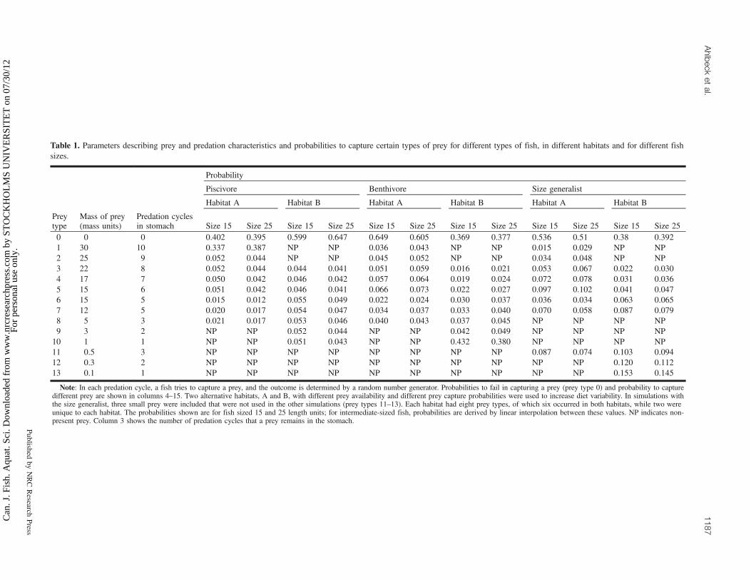
Table 1. Parameters describing prey and predation characteristics and probabilities to capture certain types of prey for different types of fish, in different habitats and for different fishsizes.
Probability
Piscivore Benthivore Size generalist
Habitat A Habitat B Habitat A Habitat B Habitat A Habitat B
Preytype
Mass of prey(mass units)
Predation cyclesin stomach Size 15 Size 25 Size 15 Size 25 Size 15 Size 25 Size 15 Size 25 Size 15 Size 25 Size 15 Size 25
0 0 0 0.402 0.395 0.599 0.647 0.649 0.605 0.369 0.377 0.536 0.51 0.38 0.3921 30 10 0.337 0.387 NP NP 0.036 0.043 NP NP 0.015 0.029 NP NP2 25 9 0.052 0.044 NP NP 0.045 0.052 NP NP 0.034 0.048 NP NP3 22 8 0.052 0.044 0.044 0.041 0.051 0.059 0.016 0.021 0.053 0.067 0.022 0.0304 17 7 0.050 0.042 0.046 0.042 0.057 0.064 0.019 0.024 0.072 0.078 0.031 0.0365 15 6 0.051 0.042 0.046 0.041 0.066 0.073 0.022 0.027 0.097 0.102 0.041 0.0476 15 5 0.015 0.012 0.055 0.049 0.022 0.024 0.030 0.037 0.036 0.034 0.063 0.0657 12 5 0.020 0.017 0.054 0.047 0.034 0.037 0.033 0.040 0.070 0.058 0.087 0.0798 5 3 0.021 0.017 0.053 0.046 0.040 0.043 0.037 0.045 NP NP NP NP9 3 2 NP NP 0.052 0.044 NP NP 0.042 0.049 NP NP NP NP
10 1 1 NP NP 0.051 0.043 NP NP 0.432 0.380 NP NP NP NP11 0.5 3 NP NP NP NP NP NP NP NP 0.087 0.074 0.103 0.09412 0.3 2 NP NP NP NP NP NP NP NP NP NP 0.120 0.11213 0.1 1 NP NP NP NP NP NP NP NP NP NP 0.153 0.145
Note: In each predation cycle, a fish tries to capture a prey, and the outcome is determined by a random number generator. Probabilities to fail in capturing a prey (prey type 0) and probability to capturedifferent prey are shown in columns 4–15. Two alternative habitats, A and B, with different prey availability and different prey capture probabilities were used to increase diet variability. In simulations withthe size generalist, three small prey were included that were not used in the other simulations (prey types 11–13). Each habitat had eight prey types, of which six occurred in both habitats, while two wereunique to each habitat. The probabilities shown are for fish sized 15 and 25 length units; for intermediate-sized fish, probabilities are derived by linear interpolation between these values. NP indicates non-present prey. Column 3 shows the number of predation cycles that a prey remains in the stomach.
Ahlbeck
etal.
1187
Publishedby
NRCResearch
Press
Can
. J. F
ish.
Aqu
at. S
ci. D
ownl
oade
d fr
om w
ww
.nrc
rese
arch
pres
s.co
m b
y ST
OC
KH
OL
MS
UN
IVE
RSI
TE
T o
n 07
/30/
12Fo
r pe
rson
al u
se o
nly.

by an amount dictated by the assumed gut evacuation rates(Table 1, column 3). After this a new predation cycle was in-itiated. When caught, these fish contained prey at differentstage of digestion. In “periodic feeding”, no evacuation tookplace during feeding. These fish types foraged until theirstomach was at least 70% full and then switched from feed-ing to evacuation (evacuating prey from the stomach accord-ing to the assumed gut evacuation rates; Table 1, column 3).The fish did not resume feeding until the stomach was empty.These fish could only be caught during the time spent forag-ing (in nature fish can be expected to be more exposed tofishing gear during its active feeding phase) and then con-tained undigested prey. If such fish were caught during theevacuation phase, diet analysis would resemble those of trap-or gillnet-caught fish with continuous feeding (described be-low).Gut evacuation in real fish results from both digestion of
food and the transport of food remains into the intestine. Inour model, these two processes were combined and referredto as evacuation. Gut evacuation rates have been describedas both linear and exponential (Jobling 1986), so we have in-cluded both in our model. When linear evacuation rates wereused, the mass of each prey was reduced by a constantamount in each predation cycle (Table 1, column 3). Withexponential evacuation, a certain fraction of the still notevacuated mass of each prey was removed in each predationcycle, which can be expressed as
masstþ1 ¼ masst � e�k
where mass was the mass of an individual prey before (t) andafter (t + 1) a predation cycle, and k was the evacuation rate.The evacuation rates were set to evacuate prey in a certainnumber of cycles, mainly in relation to its size (Table 1, col-umn 3). For linear evacuation, an individual prey disappearedfrom the stomach when its mass reached zero, while expo-nentially evacuated prey disappeared when the remainswere ≤1% of the original mass. Total evacuation time foreach prey type was identical for linear and exponential eva-cuation. We assumed that the evacuation rates were indepen-dent of the total stomach content (e.g., Temming andHerrmann 2003).
ScenariosWe simulated scenarios with piscivorous and benthivorous
fish as both continuous and periodic feeders, but the sizegeneralists were only simulated as continuous feeders, assimulations were time consuming. Those five scenarios wererun with exponential or linear evacuation, resulting in 10main scenarios. In all scenarios, stomach contents were ana-lyzed both instantaneously and after a period of stomach con-tent evacuation (described below), resulting in 20 scenarios.However, the effective numbers of scenarios were 18, be-cause by definition the gut evacuation type did not matterfor instantaneous sampling in periodic feeders, since evacua-tion did not start before the stomach analysis in these cases(Fig. 2).
Sensitivity analysisAnalysis of the different scenarios represented a form of
sensitivity analysis of the diet analysis methods. In additionto these main scenarios, we analyzed the sensitivity further,
by additional parameter changes. In terms of prey captureprobabilities, the main scenarios were supplemented withscenarios of high probability for failing to capture a prey(“High fail”), low probability for failing to capture a prey(“Low fail”), all prey having identical capture probabilities(“Generalist 1”), normal distribution of prey capture proba-bilities (the middle-sized prey most common; “General-ist 2”), and increasing capture probability with decreasingprey size (“Generalist 3”) for continuous feeders (see Ta-ble 2). In the main scenarios, the evacuation rates wereclosely coupled to prey size. To test for effects of variationin evacuation rates due to, for example, evacuation rates in-fluenced by prey tissue composition, we ran simulationswith two different versions of randomly increased or de-creased evacuation rates for continuously feeding piscivores(“Random piscivore 1” and “Random piscivore 2”) and ben-thivores (“Random benthivore 1” and “Random benthi-vore 2”) with exponential evacuation (Table 3). Theevacuation rates were krandom = koriginal·[1 + Rand(0.5)].Heavily digested prey can be difficult to identify, and to
explore effects of this, a simulation in which prey could beidentified at a mass of 10% of its original mass was run inaddition to the main scenario where 1% of original preymass was used (this simulation, “Identification level”, wasrun only for the continuously feeding benthivorous fish withexponential evacuation). Two alternative predator stomachsizes (fish length3/100 and fish length3/10) were used to in-vestigate the effect of prey numbers in the stomach (this sim-ulation, “Stomach size”, was run only for the periodicallyfeeding benthivorous fish with exponential evacuation). Wealso tested how different habitat utilization (i.e., number ofpredation cycles spent in each habitat) affected the methodresults (this simulation, “Cycles”, was run only for the con-tinuously feeding benthivorous fish). Finally, alternative preysize distributions between habitats were explored by remov-ing prey types 5 and 10 from habitat A instead of preytypes 9 and 10 and removing prey types 2 and 6 from habi-tat B instead of prey types 1 and 2 (this simulation, “Preyavailability”, was run only for the continuously feeding ben-thivorous fish). As the simulations were time consuming, wehad to restrict the number of simulations for some scenariosof the sensitivity analysis (i.e., running them only for oneprey preference, one feeding mode, and one evacuation type).Results from these additional simulations will only be dis-
cussed in relation to the sensitivity analysis, as they did notinfluence conclusions substantially.
Fish’s true dietKnowing the long-term “true” diets was critical to our
analyses. In the true diet, the “life time” consumption of thefish was registered, as opposed to the stomach content, whichpresents the prey composition at a certain time, describedabove. True diets were obtained by simulating 60 000 preda-tion cycles (initial simulations showed this to be sufficient toobtain stable diet composition) for 25 fishes from each of the11 fish sizes (15, 16,…, 25 length units), and the accumu-lated consumption was recorded for each of these individuals.For each of the 25 individuals in each size class, the dietcomposition was calculated as the mass percentages of differ-ent prey, and then the average mass percentages were calcu-lated for the size class. The true diet was then estimated as
1188 Can. J. Fish. Aquat. Sci. Vol. 69, 2012
Published by NRC Research Press
Can
. J. F
ish.
Aqu
at. S
ci. D
ownl
oade
d fr
om w
ww
.nrc
rese
arch
pres
s.co
m b
y ST
OC
KH
OL
MS
UN
IVE
RSI
TE
T o
n 07
/30/
12Fo
r pe
rson
al u
se o
nly.

the average of the average mass percentages across all 11 sizeclasses. This procedure gave fish of different size, with differ-ent amounts of consumed food, the same influence on thetrue diet. Since prey capture probabilities and evacuationrates varied among fish types, true diets were calculated sep-arately for each fish type, as described above. The resultsfrom all diet analysis methods were compared with the truediets. To visualize the modelled diet compositions and enablecomparison with real diet samples, we show the true dietcomposition per fish type (Fig. 3). Diet compositions varywidely depending on fish species and even vary within spe-cies depending on ontogeny (e.g., International Council forthe Exploration of the Sea 1997). The diet compositions gen-erated by our program fit well within the variation of real lifedata.
Sampling fish for stomach analysisA sample of fish for stomach analysis consisted of 20 fish
caught after their 1000th predation cycle. Twenty fish can beseen as a small sample size, but it is a realistic sample size inin situ samples after stratifying a larger data set into, for ex-ample, size classes, sampling sites, season, and year. To ex-plore the variation in diets derived with a certain method,we analyzed 20 samples of 20 fish each for each scenario(i.e., for all combinations of prey preference, feeding mode,
evacuation type, and sampling method; Fig. 2). To describediet variation over, for example, larger areas or longer timeperiods, 20 samples of fish is not an unrealistic assumptionand will give a reasonable estimate of variation in differentmethods. Hence, 400 fish in total (20 samples × 20 fish persample) with non-empty stomachs were analyzed for eachscenario.Two alternative sampling methods were applied. Depend-
ing on catch method used in situ, fish can be sampled andanalyzed almost instantaneously (e.g., electrofishing, explo-sives, or angling) or collected over a somewhat longer time(e.g., traps or gillnets) with the risk of fish regurgitating ordigesting some of the stomach content for hours before stom-ach content is analyzed. To simulate stomach sampling wherefish were collected instantaneously, the stomach content usedwas that present after the 1000th predation cycle but beforethe gut evacuation in this cycle had commenced. To simulatea situation where the fish could evacuate some of its stomachcontent after it was caught but before stomach analysis wasmade, the fish was allowed to evacuate its stomach contentduring a randomly determined period (0 to 5 cycles, evendistribution) before the stomach content was analyzed. If thestomach was empty when the fish was caught, an additionalfish was sampled, until 20 fish with non-empty stomachswere caught.
Continous
feeding
Exponential
digestionLinear digestion
Instantanious
sampling
e.g. electro-
shocking
Delayed
sampling
e.g. gillnets
Instantanious
sampling
e.g. electro-
shocking
Delayed
sampling
e.g. gillnets
Stomach for
piscivorous,
benthivorous
and
size generalist
Stomach for
piscivorous,
benthivorous
and
size generalist
Stomach for
piscivorous,
benthivorous
and
size generalist
Stomach for
piscivorous,
benthivorous
and
size generalist
Periodic feeding
Exponential
digestionLinear digestion
Delayed
sampling
e.g. gillnets
Delayed
sampling
e.g. gillnets
Instantanious
sampling
e.g. electro-
shocking
Stomach for
piscivorous
and
benthivorous
Stomach for
piscivorous
and
benthivorous
Stomach for
piscivorous
and
benthivorous
Prey preference
Fig. 2. Diagrammatic representation of possible fish and sampling characteristics used to derive simulated stomach contents. All these as-sumptions were used for piscivores and benthivores, but for size generalists we did not analyze scenarios with periodic feeding. In total, thisresulted in 18 sets of scenarios.
Ahlbeck et al. 1189
Published by NRC Research Press
Can
. J. F
ish.
Aqu
at. S
ci. D
ownl
oade
d fr
om w
ww
.nrc
rese
arch
pres
s.co
m b
y ST
OC
KH
OL
MS
UN
IVE
RSI
TE
T o
n 07
/30/
12Fo
r pe
rson
al u
se o
nly.

Methods
evaluatedStom
achcontentw
asanalyzed
infour
differentbasic
ways:
frequencyof
occurrence,dom
inancemethod,
numeric
meth-
ods,and
mass-based
methods.
Analternative
tousing
preymasses
couldbe
tobase
theanalyses
onprey
volumes
(Hy-
nes1950;
Swedberg
andWalburg
1970).Wehave
notex-
ploredthis
alternative,since
specificdensities
ofdifferent
preytypes
canbe
expectedto
besim
ilarand
hencealso
theoutcom
eof
thecom
parisonof
methods.Stom
achcontentw
asalso
manipulated
tomim
icdata
uncertaintyand
approximate
methods.
Furthermore,
dietswere
alsoderived
fromdifferent
composite
indices,which
combine
differentbasic
data:Per-
centIndex
ofRelative
Importance
andCom
parativeFeeding
Index.Analyses
were
made
fromindividual
stomachs,
aftermerging
stomach
content,pooled,
andafter
accountingfor
thesize
ofthe
analyzedfish,
pooledadjusted,
asdescribed
inHyslop
(1980).Abbreviations
usedbelow
areexplained
inTable
4.
Frequency
ofoccurrence
(FO)
The
proportionof
stomachs
containingeach
preytype
was
calculatedand
expressedas
apercentage
ofthe
totalnum
berof
stomachs.
Diet F
Oi
¼Nfish
;i
Nfish �
100
Dom
inancemethod
(DM)
The
proportionof
stomachs
dominated
bymass
byacer-
tainprey
typewas
calculatedand
expressedas
apercentage
ofthe
totalnum
berof
stomachs.
Diet D
M1
i¼
Nfish
;Iw
Nfish
�100
Num
ericmethod
(NM1–N
M3)
Inthis
method,
thediet
was
expressedas
thenum
ericper-
centageof
eachprey
typerelative
tothe
totalnumber
ofprey.
This
dietcould
bederived
inthree
differentways.
Innum
er-ical
method
1(N
M1),
preypercentages
were
firstcalculated
foreach
fishseparately
andthen
averagedover
allindividualsin
thesam
ple(H
yslop1980).
This
meant
thateach
fishim
-pacts
theresult
equallymuch.
Table 2. Prey capture probabilities (columns 2–20) for the for the high fail, low fail, and generalist 1–3, in different habitats and for different fish sizes, in the sensitivity analysis.
High fail Low fail Generalist 1 Generalist 2 Generalist 3
Habitat A Habitat B Habitat A Habitat B Habitat A Habitat B Habitat A Habitat B Habitat A Habitat B
Preytype
Size15
Size25
Size15
Size25
Size15
Size25
Size15
Size25
Size15
Size25
Size15
Size25
Size15
Size25
Size15
Size25
Size15
Size25
Size15
Size25
0 0.790 0.781 0.690 0.695 0.153 0.135 0.096 0.103 0.455 0.455 0.455 0.455 0.445 0.403 0.411 0.444 0.536 0.510 0.381 0.3931 0.014 0.015 NP NP 0.051 0.075 NP NP 0.068 0.068 NP NP 0.021 0.042 NP NP 0.015 0.029 NP NP2 0.023 0.024 NP NP 0.077 0.102 NP NP 0.068 0.068 NP NP 0.048 0.069 NP NP 0.034 0.048 NP NP3 0.036 0.036 0.013 0.016 0.101 0.124 0.036 0.054 0.068 0.068 0.068 0.068 0.076 0.095 0.040 0.060 0.053 0.067 0.021 0.0304 0.045 0.044 0.017 0.020 0.124 0.146 0.047 0.068 0.068 0.068 0.068 0.068 0.103 0.121 0.058 0.081 0.072 0.078 0.031 0.0365 0.060 0.057 0.022 0.026 0.155 0.166 0.058 0.076 0.068 0.068 0.068 0.068 0.138 0.155 0.076 0.101 0.097 0.102 0.041 0.0476 0.023 0.019 0.035 0.035 0.076 0.058 0.117 0.108 0.068 0.068 0.068 0.068 0.052 0.038 0.116 0.101 0.036 0.034 0.063 0.0657 0.037 0.031 0.041 0.041 0.119 0.088 0.132 0.118 0.068 0.068 0.068 0.068 0.062 0.043 0.100 0.083 0.070 0.058 0.087 0.0788 0.047 0.040 0.050 0.051 0.143 0.107 0.150 0.136 0.068 0.068 0.068 0.068 0.055 0.035 0.085 0.065 0.087 0.074 0.103 0.0949 NP NP 0.057 0.059 NP NP 0.170 0.156 NP NP 0.068 0.068 NP NP 0.067 0.044 NP NP 0.120 0.11210 NP NP 0.068 0.071 NP NP 0.194 0.180 NP NP 0.068 0.068 NP NP 0.047 0.021 NP NP 0.153 0.145
Note: In each predation cycle, a fish tries to capture a prey, and the outcome is determined by a random number generator. Probabilities to fail in capturing a prey (prey type 0) and probabilities to capturedifferent prey are shown in columns 2–20. Two alternative habitats, A and B, with different prey availability and different prey capture probabilities were used to increase diet variability. Each habitat had eightprey types, of which six occurred in both habitats, while two were unique to each habitat. The probabilities shown are for fish sized 15 and 25 length units; for intermediate sized fish, probabilities are derivedby linear interpolation between these values. NP indicates non-present prey. Prey are evacuated from the stomachs at the same rate as in the main scenarios (Table 1).
Table
3.Num
berof
cyclesthat
theprey
remained
inthe
stomach
forthe
simulations
with
randomevacuation
ratesin
thepiscivorous
andbenthivorous
fishwith
continuousexponential
evacuation.
Preytype
Random
piscivore1
Random
piscivore2
Random
benthivore1
Random
benthivore2
18
158
152
1211
1211
311
611
64
77
77
58
78
76
75
75
74
104
108
35
35
93
23
210
11
11
1190Can.
J.Fish.
Aquat.
Sci.
Vol.69,
2012
Publishedby
NRCResearch
Press
Can
. J. F
ish.
Aqu
at. S
ci. D
ownl
oade
d fr
om w
ww
.nrc
rese
arch
pres
s.co
m b
y ST
OC
KH
OL
MS
UN
IVE
RSI
TE
T o
n 07
/30/
12Fo
r pe
rson
al u
se o
nly.

DietNM1i ¼
XNfish
j¼1
Nij
N�j� 100
� �Nfish
In numerical method 2 (NM2), the stomach contents of allfish in the sample were pooled before percentages of differentprey types were calculated (Hyslop 1980). The impact ofeach fish on the result differed among fish and was propor-tional to the number of prey in the stomach.
DietNM2i ¼
XNfish
j¼1
Nij
XNfish
j¼1
N�j
� 100
Numerical method 3 (NM3) was basically the same asNM2, but before pooling prey from different stomachs, preynumbers were divided by the mass (length3) of the fish. Thisreduced the greater impact that larger fish, with on averagemore prey in their stomach, may have had.
DietNM3i ¼
XNfish
j¼1
Nij
L3jXNfish
j¼1
N�jL3j
� 100
Mass method (MM1–MM6)As with the NM, diets based on prey mass could be calcu-
lated in different ways. In mass method 1 (MM1), mass per-centages of the digested (w) prey items found in the stomachwere first calculated for each fish separately and then aver-aged over all individuals in the sample. This meant that eachfish impacted the result equally.
DietMM1i ¼
XNfish
j¼1
wij
w�j� 100
� �Nfish
In mass method 2 (MM2), the stomach contents of all fishin the sample were pooled before mass percentages of differ-ent prey were calculated (Hyslop 1980). The impact of eachfish on the result differed among fish and was proportional tothe mass of prey in the stomach.
DietMM2i ¼
XNfish
j¼1
wij
XNfish
j¼1
w�j
� 100
Mass method 3 (MM3) was basically the same as MM2,but before pooling prey from different stomachs, prey masseswere divided by the mass (length3) of the fish (adjustedpooled analysis; Hyslop 1980).
Fig. 3. The true diet compositions of the different fish types used in the 18 scenarios expressed as mass percentages of the 13 prey types(masses 30–0.1 arranged top to bottom; also see Table 1).
Ahlbeck et al. 1191
Published by NRC Research Press
Can
. J. F
ish.
Aqu
at. S
ci. D
ownl
oade
d fr
om w
ww
.nrc
rese
arch
pres
s.co
m b
y ST
OC
KH
OL
MS
UN
IVE
RSI
TE
T o
n 07
/30/
12Fo
r pe
rson
al u
se o
nly.

DietMM3i ¼
XNfish
j¼1
wij
L3jXNfish
j¼1
w�jL3j
� 100
As a modification of the three methods described above,the original prey masses (W), before digestion had started,were used for the calculations (MM4–MM6). MM4 hencecorresponded to MM1, only with original prey mass insteadof digested prey mass. Further, MM5 corresponded to MM2and MM6 corresponded to MM3 in the same way.
DietMM4i ¼
XNfish
j¼1
Wij
W�j� 100
� �Nfish
DietMM5i ¼
XNfish
j¼1
Wij
XNfish
j¼1
W�j
� 100
DietMM6i ¼
XNfish
j¼1
Wij
L3jXNfish
j¼1
W�jL3j
� 100
Approximate mass method (AMM1–AMM6)Determining the mass of different prey is time consuming
and can be associated with substantial errors if a large propor-tion of the stomach content cannot be apportioned to preytypes. To evaluate the possible impact of errors in the mass
partitioning among prey in stomachs, we introduced an errorin the mass data. This was done by multiplying the actualprey masses by a random number with an average of 1 and astandard deviation of 0.15. Based on many years of experiencein stomach analyses, we consider this degree of uncertainty inprey mass determination realistic. The approximate mass meth-ods AMM1–AMM3 corresponded to the MM1–MM3 de-scribed above, respectively, but associated with errors.In approximate mass method 1 (AMM1), digested mass
percentages were calculated, multiplied by the error value,and averaged over all individuals in the sample. Each fishimpacted the result equally:
DietAMM1i ¼
XNfish
j¼1
ewijew�j� 100
� �Nfish
In approximate mass method 2 (AMM2), the digestedstomach contents of all fish in the sample were pooled beforepercentages of different prey were calculated and the errorwas imposed. The impact of a fish was proportional to itscontribution to the total mass of prey:
DietAMM2i ¼
XNfish
j¼1
wij
!� Randð1; 0:15Þ
XNprey
i¼1
XNfish
j¼1
wij
!� Randð1; 0:15Þ
" #� 100
In approximate mass method 3 (AMM3), the size of thefish was taken into account before pooling mass data.
DietAMM3i ¼
XNfish
j¼1
ewij
L3jXNfish
j¼1
ew�jL3j
� 100
Table 4. Abbreviations used in method equations.
Rand(m,s) = normally distributed random number; mean = m and standard deviation = s
Nfish = no. of fish examinedNprey = no. of prey typesNfish,i = no. of fish that have prey of type i in the stomachNfish,Iw = no. of fish in which prey of type i dominates (i.e., has the largest mass) the stomach content, based on the masses of digested preyNij = no. of prey type i in the stomach of fish jN•j = total no. of prey in the stomach of fish jLj = length of fish jwij = mass of prey type i in the stomach of fish jw•j = total mass of prey in the stomach of fish jewij = approximate mass of prey type i in the stomach of fish j; wij × Rand(1,0.15)ew�j = the sum of approximate prey masses in the stomach of fish jWij = mass of prey type i in the stomach of fish j, based on original, undigested massesW•j = total mass of prey in the stomach of fish j, based on original, undigested mass of each preyeWij = approximate original mass of prey type i in the stomach of fish j; Wij × Rand(1,0.15)eW �j = the sum of approximate original prey masses in the stomach of fish jpij = points allotted to prey type i in the stomach of fish jp•j = total no. of points allotted to prey in the stomach of fish jpi = points allotted to prey i after merging the stomachs of all Nfish in the sampleDietXi = percentage (%) of prey i in the diet, estimated using method X
1192 Can. J. Fish. Aquat. Sci. Vol. 69, 2012
Published by NRC Research Press
Can
. J. F
ish.
Aqu
at. S
ci. D
ownl
oade
d fr
om w
ww
.nrc
rese
arch
pres
s.co
m b
y ST
OC
KH
OL
MS
UN
IVE
RSI
TE
T o
n 07
/30/
12Fo
r pe
rson
al u
se o
nly.

In this study, the original masses of each prey type weredefined, but in practice back-calculated original prey massesare associated with errors. To test for effects of this, the esti-mated masses of different prey prior to digestion were associ-ated with errors (AMM4–AMM6).In approximate mass method 4 (AMM4), original mass per-
centages, multiplied by the error value, were averaged over allindividuals in the sample. Each fish impacted the result equally:
DietAMM4i ¼
XNfish
j¼1
eWijeW �j� 100
!Nfish
In approximate mass method 5 (AMM5), the originalstomach contents of all fish in the sample were pooled beforepercentages of different prey were calculated and the errorwas imposed. The impact of a fish was proportional to itscontribution to the total back-calculated mass of prey:
DietAMM5i ¼
XNfish
j¼1
Wij
!� Randð1; 0:15Þ
XNprey
i¼1
XNfish
j¼1
Wij
!� Randð1; 0:15Þ
" #� 100
In approximate mass method 6 (AMM6), the size of thefish was taken into account before pooling mass data.
DietAMM6i ¼
XNfish
j¼1
eWij
L3jXNfish
j¼1
eW �jL3j
� 100
Points method (PM1–PM2)In this method, points were allocated to prey types in rela-
tion to their percentages of the total prey mass in the stomach(Swynnerton and Worthington 1940; cited in Hynes 1950).This allowed for less careful mass determinations than re-quired for the mass methods (MM1–MM6). In our evalua-tion, points were allotted according to Table 5. We haveused an approximately logarithmic scale, as, for example, Hy-nes (1950) and Christensen (1978) have both previously usedlogarithmic scales.These points were then treated in the same way as mass
data, both averaging over all individuals in the sample (eachfish impacts the result equally, PM1) and pooling the stom-ach content of all fish before percentages were calculatedand points were allocated (PM2).
DietPM1i ¼
XNfish
j¼1
pij
p�j� 100
� �Nfish
DietPM2i ¼ piXNprey
x¼1
px
� 100
Percent Index of Relative Importance (%IRI1–%IRI6)This composite measure combined three of the methods
mentioned above (Cortés 1997). Separately for each preytype i, diet percentages derived from the FO method(DietFOi ) were multiplied by the sum of diet percentages de-rived with one of the MM methods (DietMMx
i ) and one of theNM methods (DietNMx
i ). To calculate the percentages of preytypes in the diet, the product calculated for each prey typewas divided by the sum of all such products. The perform-ance of the %IRI method was explored using six alternativecombinations of MM and NM:
Diet%IRI1i ¼ DietFOi ðDietNM1
i þ DietMM1i ÞXNprey
x¼1
DietFOx ðDietNM1x þ DietMM1
x Þ� 100
and then for %IRI2, as for %IRI1 but using DietNM2i and
DietMM2i ; for %IRI3, as for %IRI1 but using DietNM3
i andDietMM3
i ; for %IRI4, as for %IRI1 but using DietNM1i and
DietMM4i ; for %IRI5, as for %IRI1 but using DietNM2
i andDietMM5
i ; and for %IRI6, as for %IRI1 but using DietNM3i and
DietMM6i .
Comparative Feeding Index (CFI1–CFI2)A Comparative Feeding Index (cf. Christensen 1978) was
calculated by multiplying diet percentages derived from theFO method (DietFOi ) and percentages from one of the PMmethods (DietPMx
i ). To calculate the percentages of prey typesin the diet, the product calculated for each prey type was div-ided by the sum of all such products.
DietCFI1i ¼ DietFOi � DietPM1iXNprey
x¼1
DietFOx � DietPM1x
DietCFI2i ¼ DietFOi � DietPM2iXNprey
x¼1
DietFOx � DietPM2x
Evaluation of methodsTo evaluate the performance of each method, the diet com-
Table 5. Point allocated to the mass per-centages of prey in the points method.
Percentage of mass instomach (%) Points0 0>0–1 0.5>1–2 1.5>2–4 3>4–8 6>8–16 12>16–32 24>32–64 48>64–99 82>99 100
Ahlbeck et al. 1193
Published by NRC Research Press
Can
. J. F
ish.
Aqu
at. S
ci. D
ownl
oade
d fr
om w
ww
.nrc
rese
arch
pres
s.co
m b
y ST
OC
KH
OL
MS
UN
IVE
RSI
TE
T o
n 07
/30/
12Fo
r pe
rson
al u
se o
nly.

position for each of the 20 samples of a scenario, each con-taining 20 fish with non-empty stomachs, was calculated.The similarity between each sample and the “true” diet wasthen calculated using Schoener’s similarity index (Schoener1970):
Similarity ¼XNprey
i¼1
min ðDieti; TrueiÞ
where Dieti and Truei were the percentages (%) of prey type iin the diet estimated by a particular method and in the truediet, respectively. This index produces a value of 0% at totaldissimilarity and 100% at total similarity between the diet es-timate and the true diet.The average similarity across the 20 samples of the sce-
nario was calculated for each diet analysis method, and thenthe average similarity was calculated across all 18 scenarios(Fig. 4): Further, we derived two measures of robustness ofthe methods across the 18 scenarios:
ðaÞ variationa ¼ average½st: devðsimilarityÞ�where st. dev was the standard deviation of the 20 similarityindices calculated from each of the 20 samples of each sce-nario derived by a certain method. The average of these stan-dard deviations was then calculated across the 18 scenarios.A high value on variationa implies that the method generallyproduced substantial differences in diet estimates amongsamples of fish with the same characteristics and samplingmethod. The second measured is as follows:
ðbÞ variationb ¼ st: dev½averageðsimilarityÞ�and measures the variation in the average similarity over the20 samples among the 18 scenarios. A high value of varia-tionb implies that the method produces substantial differencesin diet estimates among different scenarios (i.e., types of fishor sampling methods).The best diet analysis methods should have high values for
similarity and low values for variationa and variationb. Allsimulations were done in MATLAB 7.5.0 (The MathWorksInc., Natick, Massachusetts).
Results and discussion
The basic methods (FO, DM, NM, MM, AMM, and PM)produced diet estimates that were on average more similar tothe true diets than were the estimates of the composite indi-ces (%IRI and CFI; Fig. 4). Unsurprisingly, the mass-basedmethods, traditionally used for energetic–nutritional diet com-position, were the ones that described diets most accurately;it is, however, noteworthy that some non-mass-based meth-ods were also describing diets well.There were some general patterns of prey over- and under-
estimation for the different methods. Small and rare preywere substantially overestimated by some methods, whereasthe percentages of large and common prey were less biased(Fig. 5). Individually analyzed mass-based methods (MM1,MM4, AMM1, AMM4, and PM1) generally overestimatedsmall prey (Figs. 5a, 5c), but large overestimations of smallprey were also derived with FO, NM, and occasionally withDM (Figs. 5a, 5c).
Mass method, approximate mass method, and pointsmethodAs expected, given that the true diets were expressed in
mass, the mass-based methods (MM, AMM, PM) were themethods that on average produced the highest similarities,with low variation both among scenarios (variationb, Fig. 4)and among samples (variationa, Fig. 4). A low variationbmeans that the method performed equally well for differentpredator types and sampling techniques, hence being a goodmethod to use if little is known about the characteristics ofthe fish. A low variationa means that the method gave similarresults for each of the 20 fish samples, thus implying that themethod is feasible to use with a relatively small sample size.Although the difference in performance among the mass-based methods was small, with no great distinction amongthem, some patterns did emerge. The MM and AMM usingback-calculated prey masses (MM4–MM6, AMM4–AMM6)generally had slightly higher similarities than the correspond-ing methods with digested prey masses (MM1–MM3,AMM1–AMM3; Fig. 4). The MM and AMM with pooledanalyses and back-calculated prey masses (MM5–MM6,AMM5–AMM6) gave the highest similarities to the true di-ets, as they increased the diet percentage of large prey(Figs. 5b, 5d). The MM and AMM with individual analyses(MM1, MM4, AMM1, AMM4) performed almost as well(Fig. 4) and were slightly more robust (lower among scenariovariation, variationb; Fig. 4). The pooled analyses based ondigested prey masses (MM2–MM3, AMM2–AMM3) hadboth slightly lower similarities and slightly higher variationbthan the individually analyzed methods (Fig. 4). The AMMfollows the MM closely, indicating that the error induced did
CFI1
DM
IRI1
PM1
AMM1
MM1
NM1
FO
IRI4
AMM4
MM4
IRI3
AMM3MM3
CFI2
IRI2
PM2AMM2
MM2
NM3
IRI6
AMM6MM6
NM2
IRI5
AMM5MM5
68 70 72 74 76 78 80
4
6
8
10
12
14
Average similarity (%)
Va
ria
tio
nb
Fig. 4. The average similarity of the diet analysis methods over the18 scenarios. The sizes of the symbols are proportional to variationa.A high value on variationa (larger symbols) implies that a methodproduced substantial diet differences among samples of fish with thesame characteristics and sampling method (e.g., among samples ofpiscivorous fish with instantaneous sampling). A high value on var-iationb implies that a method produced substantial diet differencesamong different fish types (i.e., between all piscivorous fish, benthi-vorous fish, and size generalist fish). The smaller the symbols areand the closer a method is positioned to the lower right corner, thebetter is its performance.
1194 Can. J. Fish. Aquat. Sci. Vol. 69, 2012
Published by NRC Research Press
Can
. J. F
ish.
Aqu
at. S
ci. D
ownl
oade
d fr
om w
ww
.nrc
rese
arch
pres
s.co
m b
y ST
OC
KH
OL
MS
UN
IVE
RSI
TE
T o
n 07
/30/
12Fo
r pe
rson
al u
se o
nly.

0.1
1
10
FO
DM
NM
1
NM
2
NM
3M
M1
MM
2M
M3
MM
4M
M5
MM
6A
MM
1
AM
M2
AM
M3
AM
M4
AM
M5
AM
M6
PM
1P
M2
IRI1
IRI2
IRI3
IRI4
IRI5
IRI6
CF
I1
CF
I2
0.01
0.1
1
10
100
FO
DM
NM
1
NM
2
NM
3
MM
1
MM
2
MM
3
MM
4
MM
5
MM
6
AM
M1
AM
M2
AM
M3
AM
M4
AM
M5
AM
M6
PM
1
PM
2
IRI1
IRI2
IRI3
IRI4
IRI5
IRI6
CF
I1
CF
I2
0.01
0.1
1
10
FO
DM
NM
1
NM
2
NM
3
MM
1
MM
2
MM
3
MM
4
MM
5
MM
6
AM
M1
AM
M2
AM
M3
AM
M4
AM
M5
AM
M6
PM
1
PM
2
IRI1
IRI2
IRI3
IRI4
IRI5
IRI6
CF
I1
CF
I2
instantanious sampling
Meth
od
valu
e/d
ietvalu
e
Method
0.01
0.1
1
10
100
FO
DM
NM
1
NM
2
NM
3
MM
1
MM
2
MM
3
MM
4
MM
5
MM
6
AM
M1
AM
M2
AM
M3
AM
M4
AM
M5
AM
M6
PM
1
PM
2
IRI1
IRI2
IRI3
IRI4
IRI5
IRI6
CF
I1
CF
I2
True value=0
True value=0
(a)
(b)
(d)
(c)
linear evacuation,
delayed sampling
exponential evacuation,
delayed sampling
piscivore benthivore
true diet
piscivore size generalistbenthivore
exponential evacuation,
delayed sampling
linear evacuation,
instantaneous sampling
exponential evacuation,
instantaneous sampling
linear evacuation,
delayed sampling
true diet
Fig. 5. The over- and under-estimations of the smallest and the largest prey made by the methods compared with the true diet: (a) small preyin continuously feeding fish; (b) large prey in continuously feeding fish; (c) small prey in periodically feeding fish; (d) large prey in periodi-cally feeding fish. The value of the y axis is the ratio between the estimated and the true mass percentages of a prey type in the diet.
Ahlbeck et al. 1195
Published by NRC Research Press
Can
. J. F
ish.
Aqu
at. S
ci. D
ownl
oade
d fr
om w
ww
.nrc
rese
arch
pres
s.co
m b
y ST
OC
KH
OL
MS
UN
IVE
RSI
TE
T o
n 07
/30/
12Fo
r pe
rson
al u
se o
nly.

not affect the method to any great extent. The individuallyanalyzed PM1 had, as could be expected, higher similaritythan the pooled version, PM2 (Fig. 4), the reason being thatin PM1 the approximate points estimates were averaged over20 stomachs, while in the pooled analysis the approximatepoints estimates were made directly from the pooled stomachcontent.The true diets were calculated as the average of the origi-
nal prey masses of individual fish (i.e., in the same way asthe individually analyzed mass methods). Not surprisinglythen, MM4 and AMM4 were among the most similar to thetrue diets; however, MM5–MM6 and AMM5–AMM6 were,despite this, slightly more similar to the true diets, as theygenerally overestimated the largest, and energetically mostimportant, prey rather than underestimated these prey, asMM1, MM4, AMM1, and AMM4 did.If we look at the results in more detail, we can see differ-
ences between feeding modes and evacuation types. In simu-lations of continuous feeding, the individually analyzed mass-based methods (MM1, MM4, AMM1, AMM4, and PM1), incontrast with pooled analyses, generally greatly overestimatedsmall prey (Fig. 5a) and underestimated large prey (Fig. 5b).The reason for this is that stomachs containing only a fewsmall prey are given the same importance as stomachs filledwith large prey. Hence, for continuously feeding fish, it couldbe better to use individual analysis rather than pooled analy-ses, since the overestimation of small prey by individuallyanalyzed methods (Figs. 5a, 5b) could compensate for thefast evacuation rate of small prey. In simulations of periodicfeeding, on the other hand, small prey were not overestimatedto the same extent by individually analyzed mass-basedmethods, since stomachs containing only a few prey weremore unlikely, as evacuation did not start before stomachswere filled to at least 70%. In simulations of periodic feedingwhere small prey could be numerous, the pooled mass-basedmethods produced diets more similar to the true diets(Fig. 6), as they generally overestimated the small prey to alesser degree and underestimated large prey to a lesser degreethan the individually analyzed methods (Figs. 5c, 5d). For thesize generalist, however, the pooled methods generally pro-duced better results than individually analyzed methods evenfor continuous evacuation, since the smallest prey contributedvery little to the total diet by mass and were overestimated toa lesser degree by pooled methods.In simulations of fish with exponential evacuation rates,
methods using original prey masses generally produced dietscloser to the true diets than corresponding methods using di-gested prey masses for both continuous and periodic feeding(Fig. 6). This is due to the fact that a large fraction of theprey was evacuated shortly after ingestion in exponentialevacuation. For continuous feeding, original prey masses re-sulted in a slightly greater overestimation of large prey and agreater underestimation for small prey than if digested preymass methods were used (Figs. 5a, 5b).This is because, forexample, the largest prey could have been be partly digestedin the stomach at the sampling (1000th cycle), and their dietpercentage could therefore have increased when converted tooriginal mass, but the smallest prey had no potential to in-crease their percentage in the diet, as it was completely di-gested under one predation cycle. Also in simulations ofperiodic feeding, small prey got a higher estimate by using
digested masses (Figs. 5c, 5d) for the same reason as ex-plained above. Hence, original prey masses should be usedin exponentially evacuating fish.
Frequency of occurrence, dominance, and numericmethodsFO, DM, and NM produced average similarities closer to
the mass-based methods than the composite indices (Fig. 4)despite the fact that they did not consider mass properties.The methods with lowest among scenario variation (varia-tionb) were FO and DM (Fig. 4). FO generally producedhigh similarities with the true diets for all predator types andhence had a low variationb. However, its performance (simi-larity) relative to the other methods was more variable, beingmost similar or least similar to the true diets depending onfish type (Fig. 6). NM had the highest among scenario varia-tion (variationb; Fig. 4) performing well in some scenariosand poorly in others, also in relation to the other methods(Fig. 6).The large overestimation of small prey derived with FO
and NM, both in simulations of continuously and periodicallyfeeding fish (Figs. 5a, 5c), can be explained by both methodsgiving the same “importance” to all prey irrespective of theirmass; hence, the diet contribution of small prey became over-estimated. For the same reason, these methods underesti-mated the diet contribution of larger prey (Figs. 5b, 5d).This caused FO to produce lower similarities to the true dietsin piscivorous fish than did other methods (Fig. 6). Becauseof the overestimation of small prey (Figs. 5a, 5c), FO alsohad a somewhat lower similarity relative to the MM, AMM,and PM methods for the size generalist, especially for linearevacuation (Fig. 6).The NM methods gave high similarities relative to the
other methods in simulations of piscivorous and benthivorousfish with continuous feeding and delayed sampling, but gavesomewhat lower similarities for the size generalist, particu-larly for linear evacuation (Fig. 6), again owing to the over-estimation of small prey. The NM methods were hencesensitive to the prey size composition. As prey size rangewas larger in the size generalist compared with the piscivoreand benthivore, it resulted in a decreased similarity for theNM compared with the other methods (Fig. 6), as the small-est prey now contributed even less to the total prey mass butstill had the same “importance” in numbers.The NM and FO methods also had lower similarities
(Fig. 6) and higher variationa (Fig. 4) in simulations of peri-odically feeding fish, as small prey, that did not dominate interms of mass, were nevertheless often numerous in stomachsof that kind of fish. During simulations of continuous evacua-tion, on the other hand, small prey disappeared from thestomachs quickly because of their high evacuation rate andthe overestimations of small prey by NM; therefore, FO wereto some extent compensated for during these conditions. Sim-ilarities determined by NM and FO increased in all simula-tions of delayed catch (Fig. 6b) compared with simulations ofinstantaneous catch for the same reason. However, periodicfeeding still had lower similarity than continuous feeding.NM performed opposite to the mass-based methods when
it came to using pooled or individual analysis in the differentfeeding modes. Pooled NM methods were somewhat betterthan the individual NM for simulations of continuous feeding
1196 Can. J. Fish. Aquat. Sci. Vol. 69, 2012
Published by NRC Research Press
Can
. J. F
ish.
Aqu
at. S
ci. D
ownl
oade
d fr
om w
ww
.nrc
rese
arch
pres
s.co
m b
y ST
OC
KH
OL
MS
UN
IVE
RSI
TE
T o
n 07
/30/
12Fo
r pe
rson
al u
se o
nly.

30
40
50
60
70
80
90
100
FO
DM
NM
1
NM
2
NM
3
MM
1
MM
2
MM
3
MM
4
MM
5
MM
6
AM
M1
AM
M2
AM
M3
AM
M4
AM
M5
AM
M6
PM
1
PM
2
IRI1
IRI2
IRI3
IRI4
IRI5
IRI6
CF
I1
CF
I2
piscivore benthivore size generalist
linear evacuation, continuous feeding
exponential evacuation, continuous feeding
linear evacuation, periodic feeding
Sim
ilarity
with
true
die
ts(%
)
Method
30
40
50
60
70
80
90
100
FO
DM
NM
1
NM
2
NM
3
MM
1
MM
2
MM
3
MM
4
MM
5
MM
6
AM
M1
AM
M2
AM
M3
AM
M4
AM
M5
AM
M6
PM
1
PM
2
IRI1
IRI2
IRI3
IRI4
IRI5
IRI6
CF
I1
CF
I2
(b)
(a)exponential evacuation, periodic feeding
Fig. 6. The performance of all methods relative to each other for piscivorous, benthivorous, and size generalist fish types for (a) instantaneoussampling (e.g., electro fishing) and (b) delayed sampling (e.g., gillnets or traps). During periodic feeding, the instantaneous sampling producesidentical results for digested and back-calculated prey mass, as no evacuation has occurred when the fish is caught.
Ahlbeck et al. 1197
Published by NRC Research Press
Can
. J. F
ish.
Aqu
at. S
ci. D
ownl
oade
d fr
om w
ww
.nrc
rese
arch
pres
s.co
m b
y ST
OC
KH
OL
MS
UN
IVE
RSI
TE
T o
n 07
/30/
12Fo
r pe
rson
al u
se o
nly.

(Fig. 6), as the overestimation of small prey relative to largerprey was reduced in this way (Figs. 5a, 5b), but during sim-ulations of periodic feeding, individual NM was better(Fig. 6). The DM showed a stable similarity index acrossfish types (variationb; Fig. 4) and usually performed moder-ately compared with the other methods (Fig. 6). It often over-estimated small prey in simulations of continuous feeding,especially for piscivores and size generalists, but in somecases small prey were instead estimated to zero (Fig. 5a).The smallest prey very seldom dominate the stomach contentof individual fish, but when they did it gave a large overesti-mation, as those prey contributed little to the total diet.
Index of Relative Importance and Comparative FeedingIndexThe composite indices performed consistently poor in rela-
tion to the other methods (Fig. 4, Fig. 6). The %IRI had highamong scenario variation (variationb; Fig. 4), being sensitiveto fish characteristics, and also high among sample variation(variationa; Fig. 4) as did CFI (variationa; Fig. 4), indicatingthat larger samples are needed to produce a robust diet com-position estimate with theses methods.The composite indices generally overestimated small prey
in the size generalist and the benthivorous fish (Figs. 5a,5c). The methods showed slightly opposite patterns for theestimation of large prey depending on fish type, both in sim-ulations of continuous and periodic feeding (Figs. 5b, 5d).The %IRI consists of three component methods (FO, NM,and MM), which in the combination of the %IRI (%IRI =FO × (%NM + %MM)) gave lower similarities than the com-ponent methods did when used separately (Fig. 4). To assesswhy the %IRI behaved this way, the component methodswere removed one at a time and any two of the remainingmethods were combined (%NM + %MM or FO × %NM orFO × %MM) and thereafter compared with each other andwith the %IRI. The combination %NM + %MM performedconsiderably better than the combinations involving multipli-cation in all fish types. This indicates that the multiplicationof methods is problematic. The CFI is a multiplication of FOand PM, again resulting in diets less similar to the true dietsthan the component methods arrived at when used separately.Hence, multiplication of methods, also discussed by Hyslop(1980), should be avoided, since this tends to amplify theover- or under-estimation of prey.Analyzing pooled samples commonly produced lower
among sample variation (variationa) than analyses based onindividual fish for all 27 methods (Fig. 4). However, %IRIand CFI had higher variationa than the other methods bothas pooled and individually analyzed, having about 50% largervariation than the mass-based methods (Fig. 4). Variationbwas more variable, but was higher in the pooled methods ofNM, MM, AMM, and PM.
Results of sensitivity analysisThe parameterization of the model fish was made to pro-
duce certain diet compositions and stomachs with realisticvariation in prey composition and not in an effort to mimicthe reality of fish foraging. To evaluate if the parameteriza-tion influenced the model outcome and hence our conclu-sions, we evaluated the diet analyses methods for a widerange of parameter values. This resulted in fish and environ-
ments with different characteristics (Table 1). As discussed inthe Materials and methods section, we extended the explora-tion of the sensitivity of our findings in the main scenariosby using additional differences in parameter settings in themodel (Table 6). The additional prey capture probabilities(Table 2) produced virtually the same results as the main sce-narios (Table 6), with basic methods (FO, NM, MM, AMM,PM) producing results more similar to the true diets than thecomposite indices (%IRI, CFI). DM varied some in relationto the other methods.In addition to the effect of evacuation rates explored in the
simulations of periodic versus continuous feeding, simula-tions with two different versions of random evacuation rateswere explored for the piscivorous and benthivorous fish withcontinuous exponential evacuation (Table 3). In simulationsof the benthivorous fish, the pooled mass-based methods us-ing digested prey masses (MM2–MM3, AMM2–AMM3,PM2) in one case (random benthivore 1; Table 3) producedsimilarities as low as those produced by the %IRI and CFI(Table 6). The explanation is that smaller prey could remainlonger in the stomach than larger prey when evacuation wasrandom and the use of digested prey masses could then biasthe results substantially. In simulations of the piscivorousfish, the method’s performances in relation to each other re-mained similar to simulations with original evacuation ratesas long as the largest prey were having longer passage timesthan smaller prey. However, when the largest prey had ashorter passage time (random piscivore 1; Table 3), the NMhad decreased similarities, as the largest prey become under-estimated. NM, MM2–MM3, AMM2–AMM3, and PM2were hence sensitive to evacuation rates.Prey distributions between habitats, time spent in different
habitats, and alternative least possible prey identificationmass (1% or 10% of original mass) were explored, as weretwo alternative predator stomach sizes (Table 6). None of theresults from these simulations influenced conclusions sub-stantially. As discussed above, the way the fish were sampledaffects the order of the methods just slightly.
In relation to previous findingsIn nature there are many factors that influence fish diet
composition and generate variation in stomach contentamong individuals (e.g., the size of the fish or when andwhere it feeds). A consequence of this is that large numbersof fish may have to be analyzed to derive a representativeaverage diet. At the same time, each stomach analysis can bevery time consuming, particularly if there are difficulties inidentifying and counting prey because they have been heavilymasticated or digested. Hence, easy and fast methods may bepreferable, as they will allow for more fish to be examined. Itis therefore encouraging to see that the basic methods per-form well, including the approximate points method.Different methods provide different insight into the feeding
of animals. For example, mass-based methods can provide in-formation about impact on prey population or dietary nutri-tional values, numerical methods can describe feedingbehaviour of individuals by showing number of prey taken,and FO shows population-wide food habits by showing howmany individuals of a population feeds on what prey species(Pierce and Boyle 1991; Cortés 1997). In this study we usedthem all with the objective to describe the diet in terms of
1198 Can. J. Fish. Aquat. Sci. Vol. 69, 2012
Published by NRC Research Press
Can
. J. F
ish.
Aqu
at. S
ci. D
ownl
oade
d fr
om w
ww
.nrc
rese
arch
pres
s.co
m b
y ST
OC
KH
OL
MS
UN
IVE
RSI
TE
T o
n 07
/30/
12Fo
r pe
rson
al u
se o
nly.

energetic–nutritional composition, as this is a common objec-tive in diet analysis and also basic input data in, for example,quantitative food web analyses and is frequently used inmodels such as Ecosim–Ecopath (Walters et al. 1997).Hyslop (1980) concluded in a review of methods for diet
analysis that calculations based on prey mass give the bestresults, while he criticized the points method for being toosubjective. Our findings are reasonably consistent with this.The mass-based methods produced diets that were consis-tently more similar to the true diets than the other methods.However, we conclude that the PM with an approximatelylogarithmic scale (e.g., Hynes 1950 and Christensen 1978previously used logarithmic scales) mirrors the diet well(Fig. 4). This method has the advantage of being faster thanMM.Despite our focus on diet composition expressed in mass,
the FO and the NM performed surprisingly well. The NMmethods were, however, more variable than the mass-basedmethods, strongly influenced by feeding mode and preytraits. In nature, digestion rates are influenced by a numberof factors like periods of food deprivation (Elliott 1972; cf.Hyslop 1980), temperature (Reimers 1957), and prey qual-ities like energy content (Jobling 1980) and hard or indigesti-ble body parts (Hess and Rainwater 1939). These factors maythen particularly impact diets calculated from frequency ofoccurrence and numbers in the stomachs. The FO has earlierbeen criticized for ignoring the relative amounts of prey(Hyslop 1980) and exaggerating the importance of incidentalprey and prey with a long passage time due to hard bodyparts (Pierce and Boyle 1991). This is in accordance withour simulations, as seen in the simulations of the piscivorous,periodically feeding fish. In this type of fish, small prey wererare and there was no digestion during feeding, making smallprey stay as long as large prey in the stomach, resulting in
overestimation of small prey (Fig. 5c), as they are “weighted”the same irrespective of their number or mass because FOonly measures presence or absence, making FO performpoorly (Fig. 6). The NM methods have been criticized foroverestimating small prey taken in large numbers (Hyslop1980), and not surprisingly this is confirmed by our simula-tions, as the NM methods performed worse in the size gener-alist fish, where prey size differences were large, and in fishwith periodic feeding, when small prey were present in largernumbers in the stomach.Fish with large numbers of prey in the stomach, like zoo-
planktivores, were not simulated in this study. The diet of azooplanktivorous fish could, however, be seen as an extrapo-lation of the periodically feeding benthivorous fish, indicatingthat the NM would perform poorly for zooplanktivorous fish.This is also emphasized by Hyslop (1980). Prey with longpassage time will also be overestimated by the NM accordingto Hyslop (1980). This is shown in the simulations of the pe-riodically feeding fish where the smaller prey got overesti-mated because of the absence of evacuation during feedingin this scenario. In practice, a problem with NM is the diffi-culty of counting the number of prey when prey are thor-oughly masticated, digested, or do not appear in discreteunits like detritus (Hyslop 1980). The simulations comparingpossible prey identified at a level of 1% of original prey massversus 10% of original prey mass addresses some of theseproblems. We found that there was no difference in the rela-tive performance of the methods between these two identifi-cation thresholds. Generally speaking, the FO and the NMmethods are easy to use, fast, and do not require time con-suming mass determinations or other measurements of prey.However, these methods had on average lower similarity in-dices and (or) were less robust (Fig. 4, Fig. 6), making othermethods more reliable.
Table 6. The different simulations run in the sensitivity analysis.
Simulation Parameter changed Range of changeResult compared with mainscenarios
Generalist 1 Prey probabilities See Table 2 Similar to benthivoreGeneralist 2 Prey probabilities See Table 2 Similar to benthivoreGeneralist 3 Prey probabilities See Table 2 Similar to benthivoreHigh fail Prey probabilities See Table 2 Similar to benthivoreLow fail Prey probabilities See Table 2 Similar to benthivoreRandom piscivore 1 Prey evacuation rates
krandom = koriginal·[1 + Rand(0.5)]See Table 3 Decreased NM compared
with piscivoreRandom piscivore 2 Prey evacuation rates
krandom = koriginal·[1 + Rand(0.5)]See Table 3 Similar to piscivore
Random benthivore 1 Prey evacuation rateskrandom = koriginal·[1 + Rand(0.5)]
See Table 3 Decreased MM2–MM3,AMM2–AMM3, and PM2compared with benthivore
Random benthivore 2 Prey evacuation rateskrandom = koriginal·[1 + Rand(0.5)]
See Table 3 Similar to benthivore
Identification level Prey identification level Identification of prey at 10% instead of 1% Similar to benthivoreStomach size Predator stomach size From L3/100 to L3/10 Similar to benthivoreCycles No. of predation cycles in each
habitatFrom 50%/50% to 30%/70% Similar to benthivore
Prey availability Available prey types in eachhabitat
Prey types 5, 10 (Habitat A) and 1, 6 (Habi-tat B) missing instead of prey types 1, 2(Habitat A) and 9, 10 (Habitat B)
Similar to benthivore
Note: “Parameter changed” indicates which parameter was changed, “Range of change” indicates how much the parameter was changed, and “Resultcompared with main scenarios” indicates how this change affected the performance of the method in relation to the main scenarios.
Ahlbeck et al. 1199
Published by NRC Research Press
Can
. J. F
ish.
Aqu
at. S
ci. D
ownl
oade
d fr
om w
ww
.nrc
rese
arch
pres
s.co
m b
y ST
OC
KH
OL
MS
UN
IVE
RSI
TE
T o
n 07
/30/
12Fo
r pe
rson
al u
se o
nly.

Hyslop (1980) further debates the reliability of indices like%IRI in his review. An index incorporating values from dif-ferent methods should be more representative according tosome authors (Windell 1971; Cortés 1997), as several meas-urements are incorporated. Hyslop seems sceptical towardsthis, pointing out the increasing number of error sources.Bigg and Perez (1985) also uphold the shortcomings of suchmethods because of biases from food types comprising lessthan 1% of the component methods. Bigg and Perez (1985)compared the %IRI and the simple volumetric method andfound them to perform similarly, but when doing the samecomparison using non-trace data (data disregarding bodyparts that are more resistant to digestion like squid beaks),the %IRI method gave deviating results compared with thevolumetric method. Hansson (1998) criticizes the %IRImethod for producing variable results depending on the taxo-nomic resolution. Our simulations show that the %IRImethod, together with the CFI method, generally producesdiets that deviate more from the true diet compositions thanthe other methods, likely because of the multiplication ofdiet percentages derived from other diet analysis methods(discussed above).In this model, foraging is assumed to be the fish’s only ac-
tivity. In real life, this is of course not the case. For example,social interactions like inter- and intra-specific competitionwill occur. During competition, fish have been shown to ei-ther specialize or generalize to decrease dietary overlap (e.g.,Wiens 1993; Gabler and Amundsen 2010). This will be aproblem for methods like the NM and FO that diverge in per-formance during different scenarios; however, the mass-basedmethods (MM, AMM, PM) are quite stable and should beable to predict diets accurately even if fish pursue differentfeeding strategies concerning prey choice or feeding mode.Another phenomenon occurring in nature is ontogenetic dietshifts. This is not addressed in this study because the diet dif-ference between the smallest and largest fish (15–25 units)are not large enough to represent an ontogenetic shift. Ratherthe simulations are aimed at mirroring a sample of fish withcomparable diets, as in situ samples of fish are often dividedinto size classes where a relatively homogeneous diet is ex-pected. Even if ontogenetic diet shifts are not modelled inthis study, one of the mass-based methods should be able topredict diet composition well even in samples with fish onboth sides of a diet shift.The aim of this study was to explore how characteristics of
fish and sampling methods influenced the performance ofdifferent diet analysis methods when compared with a “true”diet of the fish. Prey preference, prey size, and evacuationrates are important factors influencing the performance ofthe diet analysis methods. Basic methods (FO, DM, NM,MM, AMM, and PM) performed on average better than com-posite indices (%IRI and CFI). FO, DM, and NM describedthe true diet surprisingly well despite it being expressed inmass; however, FO and NM varied in performance (similaritywith true diet) in relation to other methods, producing dietestimates most similar or least similar to the true diet de-pending on fish type. All MM, AMM, and PM methods pro-duced on average diet compositions most similar to the truediet and were most robust (lowest variationa and variationb).This shows that mass-based methods should be used for dietstudies aiming at describing the energetic–nutritional sources
of fish and the quantitative energy flow in food webs. Somepotential biases were noted in MM1, MM4, AMM1, AMM4,and PM1, resulting in the overestimation of small prey types.If there are not enough resources for rigorous weighing oridentification or if large or many samples are required to de-scribe diet variation over large areas, long time periods, orfor a wide size range of fish, the faster PM could be used.
AcknowledgementsWe sincerely thank the Editor, the Associate Editor, and
anonymous referees for constructive comments, which exten-sively improved earlier versions of the manuscript. This proj-ect was funded by the foundation Baltic Sea 2020.
ReferencesBigg, M.A., and Perez, M.A. 1985. Modified volume: a frequency–
volume method to assess marine mammal food habits. In Marinemammals and fisheries. Edited by J.R. Beddington, R.J.H.Beverton, D.M. Lavigne, and D. Martin. Allen & Unwin, London,UK. pp. 277–283.
Christensen, M.S. 1978. Trophic relationships in juveniles of thespecies of sparid fishes in the South African marine littoral. FishBull. 76(2): 389–401. Available from http://fishbull.noaa.gov/76-2/christensen.pdf [accessed 5 July 2011].
Cortés, E. 1997. A critical review of methods of studying fish feedingbased on analysis of stomach contents: application to elasmo-branch fishes. Can. J. Fish. Aquat. Sci. 54(3): 726–738. doi:10.1139/cjfas-54-3-726.
Elliott, J.M. 1972. Rates of gastric evacuation in brown trout, Salmotrutta L. Freshw. Biol. 2(1): 1–18. doi:10.1111/j.1365-2427.1972.tb01575.x.
Gabler, H.-M., and Amundsen, P.-A. 2010. Feeding strategies,resource utilisation and potential mechanisms for competitivecoexistence of Atlantic salmon and alpine bullhead in a sub-Arcticriver. Aquat. Ecol. 44(2): 325–336. doi:10.1007/s10452-009-9243-x.
Hansson, S. 1998. Methods of studying fish feeding: a comment.Can. J. Fish. Aquat. Sci. 55(12): 2706–2707. doi:10.1139/f98-158.
Heincke, F. 1908. Bericht über die Untersuchungen der BiologischenAnstalt auf Helgoland zur Naturgeschichte der Nutzfische. DieBeteiligung Deutschlands an der Internationalen Meeresforschung,4/5: 67–155.
Hess, A.D., and Rainwater, J.H. 1939. A method for measuring thefood preferences of trout. Copeia, 1939(3): 154–157. Availablefrom http://www.jstor.org/stable/1436810 [accessed 5 December2010].
Hynes, H.B.N. 1950. The food of fresh-water sticklebacks (Gaster-osteus aculeatus and Pygosteus pungitius), with a review ofmethods used in studies of the food of fishes. J. Anim. Ecol. 19(1):36–58. doi:10.2307/1570.
Hyslop, E.J. 1980. Stomach content analysis — a review of methodsand their application. J. Fish Biol. 17(4): 411–429. doi:10.1111/j.1095-8649.1980.tb02775.x.
International Council for the Exploration of the Sea. 1997. Report ofthe study group on multispecies model implementation in theBaltic. 4–10 December 1996, ICES, Copenhagen, Denmark. CM1997/J:2.
Jobling, M. 1980. Gastric evacuation in plaice, Pleuronectes platessaL.: effects of dietary energy level and food composition. J. FishBiol. 17(2): 187–196. doi:10.1111/j.1095-8649.1980.tb02752.x.
Jobling, M. 1986. Mythical models of gastric emptying andimplications for food consumption studies. Environ. Biol. Fishes,16(1–3): 35–50. doi:10.1007/BF00005158.
1200 Can. J. Fish. Aquat. Sci. Vol. 69, 2012
Published by NRC Research Press
Can
. J. F
ish.
Aqu
at. S
ci. D
ownl
oade
d fr
om w
ww
.nrc
rese
arch
pres
s.co
m b
y ST
OC
KH
OL
MS
UN
IVE
RSI
TE
T o
n 07
/30/
12Fo
r pe
rson
al u
se o
nly.

Pierce, G.J., and Boyle, P.R. 1991. A review of methods for dietanalysis in piscivorous marine mammals. In Oceanogr. Mar. Biol.Rev. 29. Edited by M. Barnes. Aberdeen University Press,Aberdeen, UK. pp. 409–486.
Pinkas, L., Oliphant, M.S., and Iverson, I.L.K. 1971. Food habits ofalbacore, bluefin tuna, and bonito in California waters. Fish Bull.152: 1–105.
Reimers, N. 1957. Some aspects of the relation between stream foodsand trout survival. Calif. Fish Game, 43(1): 43–69.
Schoener, T.W. 1970. Nonsynchronous spatial overlap of lizardsin patchy habitats. Ecology, 51(3): 408–418. doi:10.2307/1935376.
Swedberg, D.V., and Walburg, C.H. 1970. Spawning and early lifehistory of the freshwater drum in Lewis and Clark Lake, MissouriRiver. Trans. Am. Fish. Soc. 99(3): 560–570. doi:10.1577/1548-8659(1970)99<560:SAELHO>2.0.CO;2.
Swynnerton, G.H., and Worthington, E.B. 1940. Notes on the food of
fish in Haweswater (Westmorland). J. Anim. Ecol. 9(2): 183–187.doi:10.2307/1454.
Temming, A., and Herrmann, J.-P. 2003. Gastric evacuation in cod:prey-specific evacuation rates for use in North Sea, Baltic Sea andBarents Sea multi-species models. Fish. Res. 63(1): 21–41. doi:10.1016/S0165-7836(03)00041-9.
Walters, C.J., Christensen, V., and Pauly, D. 1997. Structuringdynamic models of exploited ecosystems from trophic mass-balanced assessments. Rev. Fish Biol. Fish. 7(2): 139–172. doi:10.1023/A:1018479526149.
Wiens, J.A. 1993. Fat times, lean times and competition amongpredators. Trends Ecol. Evol. 8(10): 348–349. doi:10.1016/0169-5347(93)90216-C. PMID:21236192.
Windell, J.T. 1971. Food analysis and rate of digestion. In Methodsfor assessment of fish production in fresh waters. 2nd ed. Edited byW.E. Ricker. Blackwell Scientific Publications, Oxford andEdinburgh, UK. pp. 215–226.
Ahlbeck et al. 1201
Published by NRC Research Press
Can
. J. F
ish.
Aqu
at. S
ci. D
ownl
oade
d fr
om w
ww
.nrc
rese
arch
pres
s.co
m b
y ST
OC
KH
OL
MS
UN
IVE
RSI
TE
T o
n 07
/30/
12Fo
r pe
rson
al u
se o
nly.