Evaluating comparable company valuation967424/FULLTEXT01.pdf · 2016-09-08 · management when allocating money for clients (Barker & Richard, 1999). Corporate valuation is therefore

Evaluating comparable company valuation

DEGREE PROJECT IN FINANCE REAL ESTATE AND FINANCE TRACK: FINANCE BACHELOR OF SCIENCE, 15 CREDITS, FIRST LEVEL

STOCKHOLM, SWEDEN 2016

- how to derive at the right multiple David Mårtensson Simon Oljemark

KTH ROYAL INSTITUTE OF TECHNOLOGY

DEPARTMENT OF REAL ESTATE AND CONSTRUCTION MANAGEMENT

Bachelor of Science Thesis

Title Evaluating comparable company valuation

- how to derive at the right multiple

Author(s) David Mårtensson

Simon Oljemark

Department The Department of Real Estate and Construction Management

Bachelor Thesis number TRITA-FOB-BoF-KANDIDAT-2016:57

Archive number 383

Supervisor Björn Berggren

Nicolaus Lundahl

Keywords Company valuation, comparable company valuation, the market approach,

the multiple approach, value drivers

Abstract

Company valuation is entering a new era; with increasing demands, more awareness and

internal resistance. As the companies who request the valuation, together with third parties,

begin to show more interest in the value statements - the analyst must be able to validate his

course of action with reliable reasoning based on substantiated data.

In this thesis, two approaches to the Comparable Company Valuation method will be

evaluated and analyzed with the use of a Case Study. Initially, the two approaches will be

applied on a Target Company, Company X, which will result in two value estimations. In

order to draw conclusions of how to derive a correct valuation and what approach that is to be

preferred in the given scenario, similar valuations were performed on six additional

companies, in the same manner as the Case Study, and compared with their respective real

market value. The valuation is based on financial data and all companies used in the study are

listed on Nasdaq Stockholm Stock Exchange.

Findings – First and foremost, results showed that a Comparable Company Valuation is very

dependent on its composed peer group. Results from the study indicated increasingly

favorable outcomes, when the peer group was similar to the Target Company. The prime

conclusions are that, with a perfectly composed peer group, in a mature industry, one of the

approaches was to be preferred. However, in an immature industry, where the requirements of

the companies used in the composed peer group have to be broadened, the latter approach

indicated favorable outcome.

Originality - This study is one of the first to compare two different approaches to the

Comparable Company Valuation method and analyze in what scenarios one approach is to be

preferred to the other.

Acknowledgement

This bachelor thesis has been written at the department of Real Estate and Construction and

Centre for Banking and Finance during the spring of 2016 as part of the programme Real

Estate and Finance at KTH Royal Institute of Technology in Stockholm, Sweden.

First and foremost, we would like to express our deepest gratitude to our supervisors Björn

Berggren and Nicolaus Lundahl for their assistance, patience, constructive and honest

comments and suggestions.

We also want to thank our anonymous respondent for a very helpful interview, giving us

proper insights regarding company valuation in an early stage of the thesis.

Furthermore, we want to thank our friends and families for their shown interest and support.

June 2016, Stockholm

David Mårtensson

Simon Oljemark

Examensarbete

Titel

Författare

Institution

En analys av jämförande företagsvärdering

- att nå fram till rätt multipel David Mårtensson & Simon Oljemark

Institutionen för Fastigheter och Byggande

Examensarbete Kandidat nummer TRITA-FOB-BoF-KANDIDAT-2016:57

Arkivnummer 383

Handledare Björn Berggren

Nicolaus Lundahl

Nyckelord Företagsvärdering, multipelvärdering, värdedrivare

Sammanfattning

Företagsvärdering går mot en ny era; med ökade krav, högre medvetenhet och internt

motstånd hos värderingsfirmorna. Företag som begär en värdering samt tredjeparter visar allt

mer intresse och förståelse för hur värderingen har gått till - vilket leder till att analytikern

måste redogöra för sitt tillvägagångssätt med korrekta resonemang baserade på pålitlig data.

I denna uppsats analyserar och utvärderar vi två olika approacher till Comparable Company

Valuation med hjälp av en fallstudie. Inledningsvis kommer de två approacherna utföras på

Målföretaget, Företag X, vilket leder till två olika värderingar. Vidare, för att kunna dra

slutsatser kring vilken approach som bör användas vid vilket tillfälle, gjordes liknande

värderingar på ytterligare sex företag, på samma sätt som fallstudien, dessa värderingar

jämfördes med marknadsvärdet för respektive företag. Samtliga värderingar baseras på

finansiell data och alla företag som är med i studien är listade på Nasdaq Stockholm Stock

Exchange.

Resultat – Först och främst visade resultaten att Comparable Company Valuation är väldigt

beroende av hur sammansättningen av jämförelseföretag har gått till. Resultat indikerade

vidare att värderingen gav bättre, det vill säga mer precist, resultat – om jämförelseföretagen

var lika Målföretaget. De viktigaste slutsatserna som drogs var att, när en värdering görs med

en perfekt grupp jämförelseföretag, i en mogen industri, var den ena approachen att föredra.

Vidare, på en nyare marknad, där kraven för jämförelseföretagen måste sänkas – gav den

andra approachen en mer precis värdering.

Originalitet – Denna studie är en av de första som jämför två olika approacher till

Comparable Company Valuation samt analyserar när vilken av dessa bör användas för att få

en så bra värdering som möjligt.

Table of Contents 1. Introduction ............................................................................................................................ 1

1.1 Background ....................................................................................................................... 2

1.2 Purpose ............................................................................................................................. 3

1.3 Delimitation ...................................................................................................................... 3

1.4 Thesis structure ................................................................................................................. 3

2. Theory .................................................................................................................................... 4

2.1 The Market Approach ....................................................................................................... 4

2.2 Defining value .................................................................................................................. 4

2.3 Multiples ........................................................................................................................... 5

2.3.1 Equity Multiples ......................................................................................................... 6

2.3.2 Entity Multiples ......................................................................................................... 7

2.4 Multiple Value Drivers ..................................................................................................... 8

2.5 Composing a selection of comparable companies (selecting a peer group) ..................... 9

2.5.1 Number of comparable companies ............................................................................ 9

2.5.2 Geography ................................................................................................................ 10

2.5.3 Business model ........................................................................................................ 10

2.5.4 Historical and futuristic perspective ........................................................................ 10

2.6 Risk ................................................................................................................................. 11

2.6.1 Small Stock Premium .............................................................................................. 11

2.6.2 Company Specific Risks .......................................................................................... 11

3. Methodology ........................................................................................................................ 12

3.1 Choice of method............................................................................................................ 12

3.2 The Case Study ............................................................................................................... 12

3.2.1 Traditional Comparable Company Valuation .......................................................... 12

3.2.2 Alternative Comparable Company Valuation .......................................................... 13

3.3 Data ................................................................................................................................. 13

3.4 Interviews ....................................................................................................................... 13

3.5 Simple linear regression ................................................................................................. 14

3.5.1 Interpreting the output .............................................................................................. 15

4.0 Results ................................................................................................................................ 16

4.1 Case Study ...................................................................................................................... 16

4.2 The Target Company and its composed peer group ....................................................... 16

4.2.1 The Target Company ............................................................................................... 16

4.2.2 The composed peer group ........................................................................................ 17

4.4 Multiples and their respective value drivers ................................................................... 22

4.5 Scrubbing process ........................................................................................................... 24

4.6 The Traditional Comparable Company Valuation ......................................................... 24

4.6.1 Value estimation derived from the price-to-earnings, P/E multiple ........................ 24

4.6.2 Value estimation derived from the Enterprise-to-EBITDA, EV/EBITDA multiple 25

4.6.3 Value estimation derived from the Enterprise-to-EBIT, EV/EBIT multiple ........... 25

4.6.4 Summary of the traditionally estimated values ........................................................ 26

4.7 The Alternative Comparable Company Valuation ......................................................... 27

4.7.1 Value estimation derived from the price-to-earnings, P/E multiple ........................ 27

4.7.2 Value estimation derived from the enterprise-to-EBITDA, EV/EBITDA multiple 29

4.7.3 Value estimation derived from the enterprise-to-EBIT, EV/EBIT multiple ............ 31

4.8 Comparing the outcome of the two approaches ............................................................. 34

4.9 Applying the two approaches on six additional companies ........................................... 35

5. Analysis ................................................................................................................................ 36

6. Conclusion ............................................................................................................................ 38

Criticism of own thesis ............................................................................................................. 39

Further studies .......................................................................................................................... 39

Bibliography ............................................................................................................................. 40

1

1. Introduction

There is much literature concerning the history of valuation and its different methodologies

that have been used overtime (Rutterford, 2004). Company valuation was initially a tool used

to assess whether it was profitable, or not, to invest in a company. It was later also used to

derive a credit rating for a company so that banks could estimate the risk of lending money to

a company (Bergling, 2014). Company valuations developed into a significant tool for

corporate finance professionals when conducting mergers and acquisitions, management

buyouts, leveraged buyouts, initial public offerings, raising capital through bonds and

restructuring of businesses (Koller, et al., 2016). It is also highly used within asset

management when allocating money for clients (Barker & Richard, 1999). Corporate

valuation is therefore frequently used on a day-to-day basis by both professionals and retail

investors. There are several methodologies used when estimating the value of a company,

which in a broader context consists of intrinsic valuation and comparable company valuation

(Barker & Richard, 1999).

Intrinsic valuation consists of the Discounted Cash Flow (DCF) analysis, which dates back to

the early works of Miller, Modigliani, Gordon and Shaprio (Capinski & Patena, 2009). The

DCF analysis converts future net cash flows to the present-day values where an investor

prefers the company that generates the largest net present value (Hussey, 1999).

The comparable company valuation is sometimes referred to as “peer comparison method” or

“the multiple approach”, where a Target Company is valued in comparison to other

companies of the same type. This approach assumes that the market is efficient which makes

it possible to measure a company’s value in reference to another company’s value.

There are several approaches to the comparable company valuation method where the one that

is most practiced by professionals is described by Matthias Meitner. The Target Company’s

value is measured by deriving multiples from a peer group. The peer group is selected by the

analyst and consists of closely comparable companies in relation to The Target Company. The

multiple is derived by extracting a mean or median multiple from the peer group, which could

later be adjusted by the analysts’ rule of thumb and personal experience (Capinski & Patena,

2009).

There is an alternative approach presented in the book Valuation: the market approach, which

is slightly different (Bernstrom, 2014). The selection process of the peer group is made in a

similar manner as in the method described by Matthias Meitner. One crucial difference is that

the analysts are to consider the multiples value drivers, both historical and forward-looking

value drivers. Studies show that valuation accuracy is improved when recognizing the value

drivers when selecting a peer group (Liu, et al., 2002). The peer groups multiples are plotted

in a scatter plot chart, versus the respective multiples primary value driver, which is derived

from the value drivers compounded estimated future growth (Suozzo, et al., 2001). A linear

regression line is drawn to capture the relationship between the multiple and its primary value

driver. The Target Company’s multiple is then derived by inserting The Target Company’s

2

value driver, the coefficient, into the equation that the linear regression line provides (Suozzo,

et al., 2001).

The comparable company valuation and the intrinsic valuation methods are widely used by

both analysts and retail investors (Capinski & Patena, 2009). The intrinsic valuation method

has been continually evaluated and developed, over time, by both practitioners and academics

whilst the comparable company valuation has been continually neglected and overlooked by

academics and academic literature (Bernstrom, 2014). Such a commonly used valuation

method deserves to be analyzed and assessed by academics.

1.1 Background Valuating a company by conducting a comparable company valuation is one of the most used

valuation methods. Deriving a value using comparable company valuation is often considered

unreliable, and therefore often ignored in research, leaving one of the most practiced valuation

methods underutilized (Bernstrom, 2014). However, one of the most common valuation

methods deserves to be scrutinized and improved, both scientifically and by practitioners.

Standard practice for company valuation is for an analyst to calculate the average or median

value multiple from a listed peer group and apply it to the base metric of The Target

Company, hence, using the result to derive value estimations for respective multiple, resulting

in three different value estimations. Illustrating a general outcome of a traditional valuation:

Figure 1. A fictional example of how a traditional valuation could look

The key question is whether the arithmetic mean represents The Target Company’s value?

One of the problems is that the value is not substantiated by any value driver from the

multiples used, solely it cannot explain how the conclusion of this value was derived.

This thesis aims to describe, assess and evaluate the comparable company valuation, which is

most commonly used, and present an alternative approach on how to derive at the right

multiple which can be substantiated by clear explanations and data.

3

1.2 Purpose The purpose with this thesis is firstly to explore and evaluate two different approaches to the

comparable company valuation method and study the outcomes generated by the two

approaches in comparison to the true market value. Secondly, to draw a conclusion of which

approach that generates the most accurate value in what respective scenarios.

The framing of the question is as follows:

In what scenarios are the two approaches to the comparable company valuation

method most applicable?

1.3 Delimitation We will limit the explanation of the multiples described in the theory chapter to the three

multiples that are used in the case study. However, we will present alternative multiples that

can be used when conducting a comparable company valuation and in what specific industries

that these multiples are to be used, but without a deep explanation. The case study will

describe how we estimate one Target Company’s value against its peer group using the two

approaches. However, additional companies’ value will be estimated but not presented, as

extensively as in the case study. The valuation of the additional companies will be valued

accordingly to the company valued in the case study; hence, the final value that has been

estimated will be provided post the case study. The companies used in the case study will be

limited to listed companies, which have shown sustainable profit over time.

1.4 Thesis structure The thesis begins with describing the background regarding comparable company valuation

and is followed by the purpose of this thesis and its limitations. Afterwards, key aspects and

theory are described regarding comparable company valuation. The methodology of this

thesis is then described. The results are presented by using a Case Study. The outcome of the

case study is then analyzed and described, followed by the conclusions that were reached in

this thesis. Additionally, the thesis ends with providing criticism and suggestions for further

studies.

4

2. Theory

This chapter initially explains the theory, real-life-practice and previous research regarding

comparable company valuation, in addition to this, all values, multiples and value drivers

used will be derived and explained.

2.1 The Market Approach The market approach is used to derive the valuation of a company based on how comparable

companies, listed on the stock exchange, are priced. Firstly, one must find comparable

companies, preferably within the same industry and with similar operations, capital structure,

risk-level and other value drivers. The value is then based on “rule of thumb” multiples based

on personal experiences and multiples derived from the comparable companies (Meitner,

2006).

The market approach can also derive the valuation of a company based on multiples derived

from company transactions. The process is similar to deriving multiples from listed

companies, however, it is more difficult to get access to relevant data, besides, company

transactions may include synergies, which are not representable to the company that is being

valued (Bernstrom, 2014).

2.2 Defining value Value is a defining measurement in a market economy. Investors invest in different types of

assets with an expectation that the asset will increase a sufficient amount of value to

compensate the investor for the risk taken when purchasing the asset. For this reason,

knowledge of how companies create value and how to measure value is vital intellectual

equipment. Companies can create financial value by investing capital raised from investors in

order to generate future cash flows at rates of return that exceeds the rate that investors

require to be paid for usage of their capital. A company that can increase revenues and deploy

more capital, meeting or exceeding the rates of return, the more value they create. Therefore,

a combination of growth and return on invested capital relative to the cost of capital is what

drives value. A company with well-defined competitive advantages can sustain significant

growth and high returns on invested capital (Koller, et al., 2016).

The enterprise value is often referred to as EV, defined as interest-bearing debt plus the

market value of equity minus excess cash (the market value of the operating/invested capital)

(Koller, et al., 2016).

The market capitalization or value of equity is often represented by the letter P, and is defined

as the market value of all outstanding shares for a company that is listed on the stock

exchange (Koller, et al., 2016).

5

2.3 Multiples This chapter describes the value-multiples that have been used in the study. The three

multiples chosen are the most commonly used multiples by analysts in real life practice

(Fernandez, 2001). We define a multiple as a ratio of a market price variable, such as a stock

price, the whole enterprise value or the market capitalization to a specific value drive such as

earnings or revenues of a firm (Schreiner & Spremann, 2007).

A proper analysis requires that one finds valid multiples for the specific industry. When

selecting peers one should consider both Equity and Entity multiples, since they descend from

different capital structure aspects.

The share price of a company, by itself, is an absolute value; hence, it is not of interest for the

valuation, instead, looking at multiples, in other words, ratios, one can compare a company

with another and further use this multiple to perform a valuation (Schmidlin, 2014).

According to Péter Harbula, below, are the most relevant valuation multiples, depending on

the industry of which the company being valued is operating in (Harbula, 2009).

Real estate: Price-to-book, Price-to-earnings

Building materials: Enterprise-to-EBITDA

Banking and insurance: Price-to-book, Price-to-earnings

Food and beverages: Enterprise-to-EBITDA, Price-to-earnings

Services: Enterprise-to-EBIT, Price-to-earnings

Energy: Enterprise-to-EBITDA, Enterprise-to-IC1

Technology: Enterprise-to-EBITDA, Enterprise-to-EBIT

Telecommunications: Enterprise-to-EBITDA, Price-to-earnings

Distribution: Enterprise-to-EBITDA, Enterprise-to-EBIT

Manufacturing: Enterprise-to-EBITDA, Price-to-FCF2

Construction: Enterprise-to-EBITDA, Price-to-earnings

Life sciences / healthcare: Enterprise-to-sales, Enterprise-to-EBITDA

Capital goods: Enterprise-to-EBITDA, Enterprise-to-EBIT

Media: Enterprise-to-EBITDA, Enterprise-to-EBIT (Harbula, 2009)

1 IC, short for Invested Capital, the total amount of that was put into the company shareholders and other parties.

2 FCF, short for Free Cash Flow, operating cash flow subtracted capital expenses

6

2.3.1 Equity Multiples

Multiples in equity, for example the most common one, the price-to-earnings-ratio, or p/e-

ratio, put the market value of a business in relation to its earnings. The only figure associated

with the equity multiples is the current market capitalization, often referred to as ‘market

cap’. Therefore the market-value-to-EBIT ratio, that is, market-value-to earnings before

interest and taxes, would not be an acceptable ratio, as Schmidlin puts it: “...because EBIT

does not serve the shareholders exclusively, but is also used to serve the demands of

creditors...” (Schmidlin, 2014).

As shareholders act with a futuristic mindset, future earnings are of interest. However, past

profits are also interesting, since an investor will look for sustainable profits, but in the end,

what counts for are the expected future results.

The structure of equity multiples are usually as follows:

𝑆ℎ𝑎𝑟𝑒 𝑝𝑟𝑖𝑐𝑒

𝑃𝑒𝑟𝑓𝑜𝑟𝑚𝑎𝑛𝑐𝑒 𝑖𝑛𝑑𝑖𝑐𝑎𝑡𝑜𝑟

Formula 1-1. A general structure of equity multiples

The Price-to-earnings, P/E multiple

As all multiples put one value in relation to another, looking at the price-to-earnings ratio, it

describes the current market valuation of a company, that is, the share price, in relation to its

earnings.

Price − to − earnings ratio =𝑀𝑎𝑟𝑘𝑒𝑡 𝐶𝑎𝑝𝑖𝑡𝑖𝑙𝑖𝑧𝑎𝑡𝑖𝑜𝑛

𝑁𝑒𝑡 𝑝𝑟𝑜𝑓𝑖𝑡=

𝑆ℎ𝑎𝑟𝑒 𝑝𝑟𝑖𝑐𝑒

𝐸𝑎𝑟𝑛𝑖𝑛𝑔𝑠 𝑝𝑒𝑟 𝑠ℎ𝑎𝑟𝑒

Formula 1-2. The P/E multiple

A P/E ratio of 20, for example, indicates that the company is currently valued at 20 times its

past (or expected) earnings. Assuming that an investor acquires the entire company, the price-

to-earnings ratio shows the number of years that it would take, with constant earnings, until

the investment was amortized (Schmidlin, 2014).

According to the S&P 500, which is an index of 500 large companies, known as the “standard

and poor” index, at the fiscal year, the average P/E ratio was about 24 (Bloomberg, 2015),

approximately 75% of the companies had a P/E ratio between 12 and 24 (Schmidlin, 2014).

7

2.3.2 Entity Multiples

To compare performance indicators investors can use entity multiples that represent all the

capital providers that are entitled to the enterprise value. The enterprise value is defined as the

market value of equity plus financial debt less cash (Koller, et al., 2016). The general question

of the entity method is: ‘How much does it cost to purchase the entire business?’ However,

any cash belonging to the company purchased belongs to the buyer, hence, reducing the

purchase price significantly (Schmidlin, 2014).

Entity multiples usually have the following structure:

𝐸𝑛𝑡𝑒𝑟𝑝𝑟𝑖𝑠𝑒 𝑣𝑎𝑙𝑢𝑒

𝑃𝑒𝑟𝑓𝑜𝑟𝑚𝑎𝑛𝑐𝑒 𝑖𝑛𝑑𝑖𝑐𝑎𝑡𝑜𝑟 (𝑏𝑒𝑓𝑜𝑟𝑒 𝑖𝑛𝑡𝑒𝑟𝑒𝑠𝑡)

Formula 1-3. A general structure of entity multiples

The Enterprise-to-EBITDA, EV/EBITDA multiple

Earnings before interest, taxes, depreciation and amortization, EBITDA, express the

operational income adjusted for depreciation and amortization, which are non-cash expenses.

As Schmidlin explains, “The EBITDA corresponds roughly to the gross cash flow, therefore,

EV/EBITDA shows an approximation of the proportion of the total value of the enterprise in

relation to the means that capital providers received” (Schmidlin, 2014).

When looking at businesses within an industry this ratio is sufficient, however, if the

companies are operating in different industries then differences can arise, since different

companies have different capital expenditures, which directly affect depreciation and

amortization expenses (Schmidlin, 2014). As Schmidlin explains further, “Companies with

high growth rates or high capital intensity display relatively high levels of depreciation,

whereas businesses in asset-light industries, for example wholesalers or internet companies,

usually report lower levels of depreciation”. These have an impact on EBITDA and therefore

on the resulting valuation…) (Schmidlin, 2014). Furthermore, the EV/EBITDA multiple gives

the investor a good insight on the businesses operative performance (Koller, et al., 2016).

EBITDA is defined as follows:

𝐸𝐵𝐼𝑇𝐷𝐴 = 𝐸𝐵𝐼𝑇 + 𝐷𝑒𝑝𝑟𝑒𝑐𝑖𝑎𝑡𝑖𝑜𝑛 𝑎𝑛𝑑 𝑎𝑚𝑜𝑟𝑡𝑖𝑧𝑎𝑡𝑖𝑜𝑛

Formula 1-4. EBITDA defined

𝐸𝑉/𝐸𝐵𝐼𝑇𝐷𝐴 = (𝐸𝑛𝑡𝑒𝑟𝑝𝑟𝑖𝑠𝑒 𝑣𝑎𝑙𝑢𝑒)/𝐸𝐵𝐼𝑇𝐷𝐴

Formula 1-5. The EV/EBITDA multiple

According to the S&P 500, at the fiscal year, the average EV/EBITDA ratio was about 20

(Bloomberg, 2015). Approximately 65% of the companies had an EV/EBITDA ratio between

8 and 18 (Schmidlin, 2014).

8

The Enterprise-to-EBIT, EV/EBIT multiple

The EV/EBIT multiple describes the enterprise value in relation to the operating earnings of a

company.

𝐸𝑉/𝐸𝐵𝐼𝑇 = (𝐸𝑛𝑡𝑒𝑟𝑝𝑟𝑖𝑠𝑒 𝑣𝑎𝑙𝑢𝑒)/𝐸𝐵𝐼𝑇

Formula 1-6. The EV/EBIT multiple

EBIT is defined as the earnings before interest and taxes. Thus, compared to EBITDA,

depreciation and amortization is excluded. Schmidlin explains: “…The ratio is particularly

suitable for comparisons of businesses across industries and serves here as a central valuation

multiple together with the price-to-earnings ratio. The EV/EBIT multiple considers the capital

structure and includes the financial stability of the firm directly in the valuation." (Schmidlin,

2014).

According to the S&P 500, at the fiscal year, the average EV/EBIT ratio was about 15

(Bloomberg, 2015), approximately 80% of the companies had an EV/EBIT ratio between 8

and 24 (Schmidlin, 2014).

2.4 Multiple Value Drivers Multiples, as those explained above, are stimulated by their respective primary value driver,

affecting their outcome over time, in addition to risk (as will be explained later in the thesis).

The value drivers are unique for different multiples. In general, a higher value driver would

result in a higher value multiple. Looking at the price-to-earnings multiple, the value driver is

the expected percentage growth of the company’s earnings after tax, derived from the

expectations of the futuristic 3 years. Similarly, the enterprise-to-EBITDA multiples value

driver is the expected percentage growth of the company’s earnings before interest, taxes,

depreciation and amortization and the enterprise-to-EBIT multiples value driver is therefore

the expected percentage growth of the company’s EBIT (Liu, et al., 2002). Note that all value

drivers are expressed in percentage.

Conclusions regarding the value drivers above can be estimated by historical data as well as

from forward-looking data provided by analysts following the listed companies (Liu, et al.,

2002).

9

2.5 Composing a selection of comparable companies (selecting a

peer group) According to a survey, 40% of analysts find the process of selecting comparable companies

problematic (Beckmann, 2003). Some practitioners call the process of selecting comparable

companies “an art form”, and that it should be left to professionals (Bhojraj, 2003). However,

this statement threatens its credibility (Bhojraj, et al., 2002). A selection of comparable

companies is referred to as a peer group. This process is nonetheless a prime task when using

a comparable company valuation. Comparable companies must have similar characteristics to

The Target Company; however, results are mixed regarding which specific characteristics

should be concordant (Meitner, 2006). Hence, having similar characteristics does not

necessarily mean that the comparable companies have to be identical to The Target Company;

however, they should be “alike” (Hickman & Petry, 1990). Considering the limited number of

public companies in reality, it becomes obvious that it is difficult to find firms that perfectly

match all criteria. Usually, companies in the same industry face the same life cycle and

competition. Having stated this, one does not find good peers just by selecting peers that

operate in the same industry. However, according to a study, valuation errors decline when

comparable companies are selected based on industry SIC-codes, also known as standard

industrial classification-codes (Alford, 1992). Other criteria that must be taken in

consideration is the market share, the size of the company and the capital structure

(Schmidlin, 2014). In case of doubt if a comparable company deviates too much from The

Target Company, one should exclude this company from the peer-group (Meitner, 2006). The

selection of relevant comparable companies (peer group) is an important step due to the fact

that the value is derived though relative valuation. The valuation might be flawed if the peer

group differs extensively from the company being valued in terms of industry, operations and

additional value drivers. (Bernstrom, 2014).

2.5.1 Number of comparable companies

The number of comparable companies required to perform a comparable company valuation

varies; generally, it is up to the analyst in terms of the product of comparability. Generally

speaking, having numerous comparable companies is preferable if they do not share the same

characteristics and are not perfectly alike. Hence, having more companies in the peer group

gives the analyst a chance to out values that deviate from the rest of the selection (Weber &

Wüstemann, 2004). Practitioners usually use a smaller number of closely selected comparable

companies whilst academic literature often uses all the companies in a specific industry as

their peer group. However, recent studies show that a peer group consisting of 5-10

companies by using a simple selection rule based on growth rates is as accurate on average as

using a peer group consisting of an entire industry (Cooper & Cordeiro, 2008).

10

2.5.2 Geography

In the process of finding a suitable peer group, it is essential to consider geographic

circumstances that may have effect on company growth. It is undisputed that macro-economic

trends such as GDP and monetary policy play a crucial part in company growth and therefore

also affects the multiples that can be derived from the peer group (Meitner, 2006). To derive

value multiples from a peer group one must find suitable peers in the same country, or at least

in counties where macro-economic trends are reasonably alike (Bernstrom, 2014). It is also

known that different regions tend to have different patterns of evolution, for example,

companies operating in Asia tend to have strong projections, not being too affected by

slowdowns, whilst Europe has shown modest, but now increasing growth (Martins, 2011).

2.5.3 Business model

The selection process also highly depends on the business model, which for the peer group

should be as similar as possible to the Target Company. A simple approach to the problem of

selecting similar comparable companies is to find companies within the same industry,

furthermore compare business models and financial rations between The Target Company and

the potential comparable companies to arrive at the adequate peer group (Henschke, et al.,

2009).

2.5.4 Historical and futuristic perspective

According to a study, where the authors analyzed companies in the same industry and their

historical growth, valuation errors were smaller when comparable companies are matched on

historical growth (Sehgal & Pandey, 1981). Another study showed similar results, looking at

forecasted growth (Zarowin, 1990). The purpose of analyzing historical financials in

combination with the specific company strategy aims to explain historical performance, both

operating and financial performance, furthermore helps one identify business risks and key

profit drivers. It is then possible to make correct estimations of future performance with

relevant historical data as a basis (Healy & Palpu, 2000). The time period of historical data

should in general cover a time period about 3-5 years if representative and relevant data is

available. The time period can be shortened or increased depending on the information that

the historical data provides, however, the time period should represent the company’s or

industries future growth and earnings potential (Bernstrom, 2014).

11

2.6 Risk Financial risk is an important factor when valuing a company. Financial risk can be thought of

as the variability in cash flows and market values that are caused by unpredictable events and

changes that are both macro-economic or company specific (Holton, 2004).

2.6.1 Small Stock Premium

It has been beneficial to invest in small companies, rather than large, and this has been

documented in numerous studies (Bis, 2007). Small Cap companies annual rate of return from

1925 to 1997 was 12,7 % while large cap companies reached an annual return of11 %,

according to Ibbotson Associates (Kathman, 1998). In 1981, Rolf Banz was able to show that

“the common stock of small firms had, on average, higher risk adjusted returns than the

common stock of larger firms”. He concluded that the size was not the likely value driver of

the over performance, rather a hidden risk (Banz & W, 1981). However, in 1986 Amihud and

Mendelson provided evidence that the illiquidity is a primary driver behind the small stock

premium (Amihud & Mendelson, 1986). Investors require higher returns on small stocks

since they in general lack liquidity, hence making it difficult to get in and out of positions

quickly in the event of a market downturn (Bis, 2007).

2.6.2 Company Specific Risks

A company can be exposed to numerous company specific risks compared to other large

traded counterparts (James, et al., 2005). These risks are, in general, priced in to the stock and

can be caused by factors such as; inexperienced management, a high dependency on one

customer or supplier, key personal or lack of customer loyalty. Companies exposed to such

risks must offer a higher rate of return to attract investors (Israel, 2011). However, analysts do

not have a general procedure for measuring company-specific risks, which means that

analysts interpret these risks differently (Meinhart, 2008).

12

3. Methodology

3.1 Choice of method This is mainly a quantitative study where both historical and futuristic data is analyzed with

mathematical and statistical models, in order to arrive at a valuation of a Target Company in a

Case Study (Höst, et al., 2006).

3.2 The Case Study We have conducted a case study, in which we have compared two different approaches used

in the comparable company valuation method. The first method described will demonstrate

the most used and practiced method whilst the second method will demonstrate a more

uncommon method.

The Target Company is usually an unlisted company; therefore robust data is hard to gather.

The process includes substantial research and interviews, however, to illustrate the process we

have, for practical and logical reasons, used an already listed company. The data used was

gathered with Bloomberg, hence, forecasts are made by professional analysts.

The case study will result in two value statements for The Target Company at the end of year

2015. The first value statement, derived from the traditional comparable company valuation

will be compared with the latter one, a value estimation calculated with the alternative

comparable company valuation method, and thus, these will be analyzed of their propriety.

3.2.1 Traditional Comparable Company Valuation

The comparable multiple-based valuation is conducted by deriving multiples from a peer

group which have similar value drivers and operate in the same, or in some cases similar,

industries and countries meaning that they are exposed to similar macro-economic conditions.

The peer group consists of listed companies (Meitner, 2006). The amount of companies in a

peer group varies depending on how many similar listed companies one can find with suitable

financial data, however, the amount of companies tends to vary amongst 5 to 10 companies

(Cooper & Cordeiro, 2008). Specific industry multiples are derived by taking the peer groups

mean or median multiple which is applied to The Target Company’s base metric. It is

common that the derived multiples are adjusted based on the analysts’ personal experience

and The Target Company’s individual risks compared to the peer groups (Meitner, 2006). A

graph containing the valuation from the derived multiples is created to get an overview of the

derived valuations. A specific value or a range is derived from the graph, sometimes using an

arithmetic mean, sometimes adjusted depending on the analysts’ recent experiences.

13

3.2.2 Alternative Comparable Company Valuation

The alternative comparable multiple-based valuation is conducted by deriving multiples from

a peer group which have similar value drivers and operate in the same, or in some cases

similar, industries and countries meaning that they are exposed to similar macro-economic

conditions. The peer group consists of listed companies (Meitner, 2006). The amount of

companies in a peer group varies depending on how many similar listed companies one can

find with suitable financial data, however, the amount of companies varies amongst 5 to 10

companies (Cooper & Cordeiro, 2008).

Specific industry multiples, from the peer group, are plotted as Y-variables, in a scatter chart,

versus its primary value driver, the X-variable, which is derived from the value drivers

compounded estimated future annual growth. A linear regression line is drawn to capture the

relationship between the multiple and its primary value driver. The Target Company’s

multiple is then derived by drawing a vertical line from its x-axis; from its compounded

estimated future annual growth in its primary value driver, until it intersects the peer groups’

linear regression line. An additional line is drawn horizontally towards the y-axis; from the

section in where the peer groups’ linear regression line was intersected, to derive the multiple

in relation to The Target Company’s compounded estimated future annual growth from its

value driver. The multiple can also be derived by inserting the X-variable into the simple

linear regression equation.

3.3 Data All historical and forecasted financial data is extracted from Bloomberg Terminal. All data

has been entered and processed in Microsoft Excel by the authors themselves. All companies

used in the thesis are listed on the Nasdaq Stockholm stock exchange.

3.4 Interviews Two interviews were conducted at an early stage of the project. Both interviews were

recorded with an audio recorder and transcribed to its full extent. Both interviews were semi-

structured and consisted of several key questions in order to define which areas to be

explored. The questions were designed in such a manner that both the respondent and the

interviewer could diverge in order to pursue interesting responses or ideas in detail. This

method was chosen because it allows one to pursue elaboration of information that is of

significance but not previously thought of as pertinent. Both authors in this bachelor thesis

were present during both interviews and both of the authors asked questions.

The first interview was conducted 24-04-2016 with an analyst at IK investment Partners

named Farhad Tatar with approximately 2 years of experience in the finance industry. Most

questions and answers were related to the comparable company valuation method and

company valuation in general. This interview lasted approximately one hour.

The second interview was conducted 11-05-2016 and the person interviewed prefers to

remain anonymous. This person has extensive experience with company valuation and has

worked in the finance industry since 2000. This interview was more focused on how to select

a peer group and how to derive at the right multiple, also clear explanations of different

approaches to the comparable company valuation method, but also, defining the differences

14

between the traditional and alternative comparable company valuation methods. This

interview lasted two hours.

The semi-structured interviews were favorable since it provided an in debt knowledge of how

comparable company valuation is practiced. The key questions and follow-up questions

provided sufficient information and many insights which helped to answer the thesis framed

question and in addition also provided great insight of how the comparable company

valuation is conducted in practice. The answers provided from the professionals also included

helpful insights in selecting academic literature, financial data and selecting the companies

used in the case study. The interviews also resulted in insights of what missteps most

practitioners make.

3.5 Simple linear regression Interpreting the data received from the alternative valuation method is rather straightforward,

however, one would like to estimate the precision of the value estimated. The perks of using a

simple linear regression are that it can be made with few observations (Simkiss, et al., u.d.).

To arrive at a valuation, using the alternative valuation method, one must derive the multiple

from a composed peer group (Bernstrom, 2014). This is possible if x and y show a

relationship with each other, one can predict y from x by establishing their relationship. The

relationship, in its simplest model, is a straight line called a simple linear regression line

where one is regressing y on x. Simple indicates that the regression line is only dependent on

one independent variable whilst linear indicates that the model used is a straight line (Dowdy,

et al., 2004). The simple linear regression line is established by plotting the pairs, x and y, as

points in a graph called scatter plot (Dowdy, et al., 2004). The points in the graph, when using

the alternative comparable company valuation method, will in general appear in a linear

upward trend since an investor is willing to pay a higher multiple for a higher estimated value

driver (Bernstrom, 2014). A simple linear regression line, is used to establish a straight line, to

fit such data so that the line can be used to predict the variable y (multiple) given the provided

x variable (the value driver, in this case the expected growth in the multiple’s performance

indicator) (Dowdy, et al., 2004). Since the slope has a linear upward trend, it measures the

change in the value of y corresponding to a unit change in the value of x (Dowdy, et al.,

2004).

The linear mean, known as the regression equation, is mathematically represented by the

formula:

𝒀 = 𝜶 + 𝜷𝚾

Formula 1-6, the simple linear regression equation

Where 𝜶 and 𝜷 are regression coefficients. The closer the regression line comes to all the

points on the scatter plot, the better it is (Simkiss, et al., u.d.). The regression equation and the

linear relationship are either calculated with a graphing calculator or with the excel add-on

‘Data Analysis’

The additional data received is as follows: df, p, s, r, r-square, adjusted r-square,

standard error, ss and ms

15

3.5.1 Interpreting the output

The measurement used to express the degree of association between x and y is the correlation

coefficient, meaning the simple linear regression line and its usefulness for predicting y at the

given x (Dowdy, et al., 2004). When determining the variability in y, which is explained by

the linear association between x and y, this is the sample coefficient of determination 𝑟2. 𝑟2 is

therefore the proportion of variability in y which is explained by the linear relationship

(Dowdy, et al., 2004). A large 𝑟2 (close to 1) indicates that the variability is explained by the

relationship, thus the knowledge of the numerical value of the x variable is almost as efficient

as knowledge of y. On the contrary, if 𝑟2is close to 0, then there is little, or no, linear

association between the two variables, hence, and information about the size of the x variable

provides very little information about the size of the y variable. A 𝑟2 value higher than 0.5

would indicate a large relationship (Dowdy, et al., 2004).

The degrees of freedom are referred to as ‘df’, which equals to the number of points

(variables) minus 2.

The probability, referred to as ‘p’ meaning this correlation is strong by chance, hence,

a p value of 0.1 would indicate that the data is significant on a 90% level.

The output ‘s’ is the standard deviation, or standard error, which is a measure of how

much the observed values of y differ from the values provided by the simple linear

regression line. Small values would indicate that the points found in the scatter plot

are close to the regression line, hence, a high value indicates scattering.

In simple linear regression, a single outcome variable is related to a single explanatory

variable by a straight line that represents the mean values of the response variable for

each value of the explanatory variable. If the line is pointing upwards, then the relation

is positive. If the line is pointing downwards, then the relation is negative.

The correlation coefficient r is used to measure the strength of association between

two variables. A value close to 1 or -1 therefore indicates a strong linear association.

A value of r close to 0 indicates a weak association (Simkiss, et al., u.d.). According to

Oxford Journal, an r value of 0.10 to 0.29 defines a small relationship, an r value of

0.30 to 0.49 defines a medium relationship and an r value of 0.5 to 1.0 defines a large

relationship. (Simkiss, et al., u.d.)

16

4.0 Results

4.1 Case Study We decided to use a case study to explain and properly illustrate the differences between the

traditional valuation method and the alternative valuation method, hence, illustrating the

process of estimating a value with the use of these two methods for the reader to understand

this matter. A case study gives good insights and further understanding of the problem in

context (Farquhar, 2012). By performing a case study, data is received to later discuss and

answer the thesis’ question framed; ‘In what scenarios are the two approaches to the

comparable company valuation method most applicable?’, including the process of how to

implement the theories in practice.

In this case study, 10 comparable companies have been selected; all companies are listed and

chosen according to the chapter “composing a selection of comparable companies (selecting a

peer-group)’, see chapter 2.5 to 2.5.4. The selected comparable companies in this study are

referred to as a “peer group”. The selected peers will be described in short below, together

with a summary of essential data to the study, presented in a table.

4.2 The Target Company and its composed peer group

4.2.1 The Target Company

The targeted company will be referred to as Company X or The Target Company; Company

X is a pump manufacturer for diversified industrials. The company designs oil pumps, water

pumps, fuel pumps and hydraulic systems. In their own words, Company X is one of the

world’s leading pump manufacturers; with global manufacturing in Sweden, Germany, UK,

USA, China and India (The Target Company, 2015).

Company X Data Summary FY-2 FY-1 FY (2015) FY+1 FY+2

Market Capilization (Msek) 3 197,8 3 942,4 4 585,2

Enterprise Value (Msek) 3 202,8 3 907,4 4 509,2

Revenues (Msek) 1 980,0 2 078,0 2 306,0 2 151,3 2 246,8

EBITDA (Msek) 409,0 406,0 477,0 431,3 465,3

EBIT (Msek) 321,0 323,0 403,0 358,8 393,3

Net Income (Msek) 176,0 241,0 271,0 248,8 276,0

Earnings Per Share 4,01 5,55 6,44 6,22 6,88

Table 3. Data extracted from Bloomberg Terminal combined with historical data found in

Company X’s annual report

17

4.2.2 The composed peer group

Initially ten companies were selected to be part of the case study, however, the data extracted

from two of these was insufficient, hence, these companies were excluded from the

calculations part of the study, the two excluded companies are still kept in the composed peer

group to illustrate the fact that “scrubbing”3 should not be performed in a too early stage of

the process.

Comparable Company 1: SKF AB

SKF AB will be referred to as “Peer 1”. Peer 1 is a supplier of products, solutions and

services within rolling bearings, seals, mechatronics, services and lubrication systems. Its

services include technical support, maintenance services and asset efficiency optimization.

Peer 2’s biggest market is in Western Europe; however, they are operational in Sweden, USA

& Asia (SKF AB, 2015).

SKF AB Data Summary FY-2 FY-1 FY (2015) FY+1 FY+2

Market Capilization (Msek) 76 818 75 087 62 474

Enterprise Value (Msek) 92 858 93 351 77 200

Revenues (Msek) 63 597 70 975 75 997 72 166 73 512

EBITDA (Msek) 10 242 11 356 12 351 10 197 10 759

EBIT (Msek) 8 349 8 964 9 493 7 983 8 508

Net Income (Msek) 3 947 5 018 5 521 4 906 5 390



Peer 2’s annual report

3 Scrubbing is the process of excluding data that is extraordinary or insufficient, in this case, scrubbing refers to

the process of excluding companies.

18

Comparable Company 2: Fagerhult AB

Fagerhult AB will be referred to as “Peer 2”. Peer 2 is engaged in developing, manufacturing

and marketing new and energy-efficient lighting solutions for professional and outdoor

environments. It provides its products to schools, offices, hospitals and other industries. Peer

2 is operational in Sweden and approximately 20 other countries in Europe and also Australia

(Fagerhult AB, 2015).

Peer 2 Data Summary FY-2 FY-1 FY (2015) FY+1 FY+2



Revenues (Msek) 3 095 3 736 3 909 4 203 4 451

EBITDA (Msek) 366 474 503 584 635

EBIT (Msek) 278 379 396 481 542

Net Income (Msek) 183 261 289 347 389




Comparable Company 3: Haldex AB

Haldex AB will be referred to as “Peer 3”. Peer 3 is engaged in development, production and

sale of brake products and air suspension systems for heavy vehicles. The company offers

disc brakes, brake adjusters and actuators, compressed air dryers, valves, ABS and EBS.

Haldex is operational in Sweden, Europe, Asia and South America (Haldex AB, 2015).




Revenues (Msek) 3 920 4 380 4 777

EBITDA (Msek) 388 660 560

EBIT (Msek) 153 408 421 358 514

Net Income (Msek) 163 238 282




19

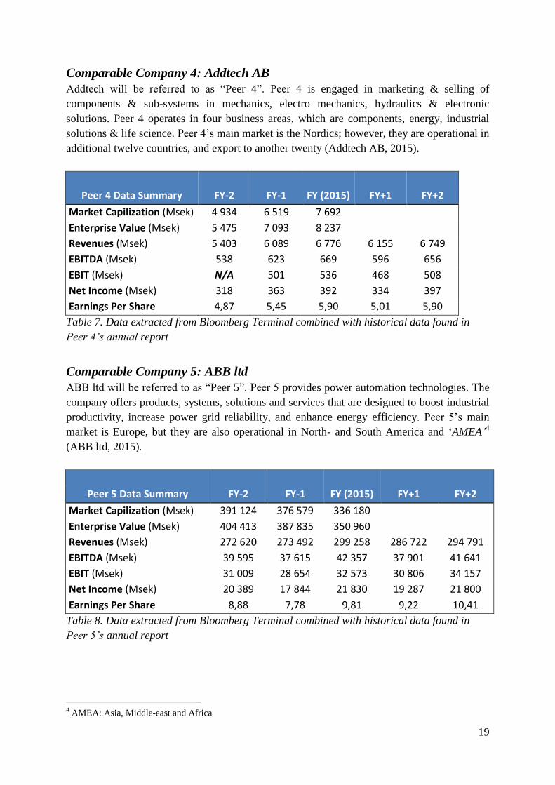
Comparable Company 4: Addtech AB

Addtech will be referred to as “Peer 4”. Peer 4 is engaged in marketing & selling of

components & sub-systems in mechanics, electro mechanics, hydraulics & electronic

solutions. Peer 4 operates in four business areas, which are components, energy, industrial

solutions & life science. Peer 4’s main market is the Nordics; however, they are operational in

additional twelve countries, and export to another twenty (Addtech AB, 2015).




Revenues (Msek) 5 403 6 089 6 776 6 155 6 749

EBITDA (Msek) 538 623 669 596 656

EBIT (Msek) N/A 501 536 468 508

Net Income (Msek) 318 363 392 334 397




Comparable Company 5: ABB ltd

ABB ltd will be referred to as “Peer 5”. Peer 5 provides power automation technologies. The

company offers products, systems, solutions and services that are designed to boost industrial

productivity, increase power grid reliability, and enhance energy efficiency. Peer 5’s main

market is Europe, but they are also operational in North- and South America and ‘AMEA’4

(ABB ltd, 2015).




Revenues (Msek) 272 620 273 492 299 258 286 722 294 791

EBITDA (Msek) 39 595 37 615 42 357 37 901 41 641

EBIT (Msek) 31 009 28 654 32 573 30 806 34 157

Net Income (Msek) 20 389 17 844 21 830 19 287 21 800




4 AMEA: Asia, Middle-east and Africa

20

Comparable Company 6: Alfa Laval AB

Alfa Laval AB will be referred to as “Peer 6”. Peer 6 is engaged in developing products &

solutions for heat transfer, separation & fluid handling. Its products are heat exchangers,

separators, pumps & valves used in oil platforms, power plants, mining, wastewater

treatment, and refrigeration. The company’s four main markets are USA, China, South Korea

& the Nordics; however, they are operational eight additional countries (Alfa Laval AB,

2015).




Revenues (Msek) 29 801 35 067 39 746 34 958 33 649

EBITDA (Msek) 5 343 6 449 7 472 6 336 6 036

EBIT (Msek) 4 336 4 980 5 711 4 825 4 623

Net Income (Msek) 3 027 3 196 3 841 3 717 3 453




Comparable Company 7: Nibe Industrier AB

Nibe Industrier AB will be referred to as “Peer 7”. Peer 7 is a Swedish heating technology

company. The company’s operating business segments are X-energy systems, X Element and

X Stoves. Peer 7 is operational in Sweden, Europe, Asia and North America, with over 10 000

employees (Nibe Industrier AB, 2015).




Revenues (Msek) 9 834 11 033 13 243 14 038 15 733

EBITDA (Msek) 1 496 1 741 2 108 2 345 2 577

EBIT (Msek) N/A N/A 1 700 1 863 2 085

Net Income (Msek) 864 988 1 243 1 356 1 524




21

Comparable Company 8: Xano Industri AB

Xano Industri AB will be referred to as “Peer 8”. Peer 8 develops, acquires, and operates

manufacturing businesses in the Nordic and Baltic regions. The company operates in

Industrial Solutions, Precision Components, Precision Technology and Rotational Molding

segments. Peer 8 is operational in Sweden, Norway, Estonia, Finland, Poland and China

(Xano Industri AB, 2015).

The data received from Bloomberg for Peer 8 was insufficient and therefore this peer did not

meet the requirements to be listed, hence, removed from the peer group.

Comparable Company 9: OEM International AB

OEM International AB will be referred to as “Peer 9”. Peer 9 is a technology trading group

acting as a link between its customers and manufacturers of products and systems for

industrial applications. Peer 9 is operational in 14 countries, including Sweden (OEM

International AB, 2015).

The data received from Bloomberg for Peer 9 was insufficient and therefore this peer did not

meet the requirements to be listed, hence, removed from the peer group.

Comparable Company 10: Autoliv Inc.

Autoliv Inc will be referred to as “Peer 10”. Peer 10 is a developer, manufacturer and supplier

to the automotive industry of automotive safety systems. The company’s products include

passive safety systems and active safety systems. Peer 10 is operational on a global level, with

a main market in Europe - totaling 64 000 associates (Autoliv Inc. , 2015).




Revenues (Msek) 57 350 63 450 77 339 84 324 90 011

EBITDA (Msek) 7 362 8 122 10 898 10 794 11 624

EBIT (Msek) 0 0 7 534 7 525 8 527

Net Income (Msek) 3 515 3 903 5 394 5 068 5 507




22

4.4 Multiples and their respective value drivers After stating that the composed peer group seems to be accurate to The Target Company, the

next step is finding proper value multiples, recalling chapter 2.3, one will want multiples

derived from both the Enterprise Value and the market value of equity, P (Bernstrom, 2014),

in other words, both Equity and Entity multiples. According to Peter Haruba and the

information presented in chapter 2, the most commonly used multiples when applying a

comparable company valuation on companies operating in either construction or services,

such as all companies in the composed peer group, are the price-to-earnings multiple, the

enterprise-to-EBITDA multiple and the enterprise-to-EBIT multiple.

Due to peer 8 and 9 being removed from the composed peer group, the number of peers is

reduced to 8 (from the previous composition of 10), of course, excluding The Target

Company.

The multiples for the fiscal year of the value estimation are derived according to the formulas

defined and explained in chapter 2.3.

Table 12. Data extracted from Bloomberg Terminal, showing the industry specific multiples

23

Furthermore, one will want to find the respective value drivers stimulating the multiples

selected. Again, recall chapter 2.4, the values affecting the derived multiples are; the

percentage growth in earnings after tax, the percentage growth in EBITDA and the percentage

growth in EBIT.

Table 13. Data extracted from Bloomberg Terminal, showing expected growth rates, the

value drivers.

As shown in table 13, the values of two peers were scrubbed, more on this in the following

chapter 4.5.

24

4.5 Scrubbing process Analysts often refer to the process of excluding and removing certain data, or in this case,

companies, as “scrubbing”. Hence, peers with extraordinary values have been scrubbed due to

their irrelevance of the correlation. Furthermore, peer 3 and 6 were removed from the case

study. Peer 3 had recently gone through substantial structural changes, making the estimation

unreliable. Peer 6 was removed to its value drivers not being aligned with the rest of the peer

group.

4.6 The Traditional Comparable Company Valuation Following the guidelines and theory of the traditional valuation method, post calculating the

median multiple of the peer group, one will want to multiply the calculated medians with their

key performance indicator (Bernstrom, 2014). This will result in 3 value estimations, derived

from 3 different multiples.

4.6.1 Value estimation derived from the price-to-earnings, P/E multiple

As mentioned above, firstly, one will estimate Company X’s value derived from the price-to-

earnings multiple. See table 12 on page 22, hence, the multiple suitable for the estimation is

the median multiple of the composed peer group.

The peers are valued at a price-to-earnings multiple in the range of 16,1x to 25,36x, with the

mean and median values of 19,97x and 20,15x. Therefore, the comparable companies’ are,

expressed in mean and median terms, valued at 19,97x and 20,15x their past reported net

income.

This provides us with the following data:

The peer groups’ median price-to-earnings multiple: 20.15x

Company X’s net income LFY: 271Msek

Furthermore, applying the median price-to-earnings multiple onto our Target Company, we

arrive at the estimated value:

𝐸𝑠𝑡𝑖𝑚𝑎𝑡𝑒𝑑 𝑉𝑎𝑙𝑢𝑒 (𝑝𝑟𝑖𝑐𝑒 − 𝑡𝑜 − 𝑒𝑎𝑟𝑛𝑖𝑛𝑔𝑠) = 20.15 𝑥 271 = 5460,65𝑀𝑆𝐸𝐾

Formula 1-7. Estimating a value from the P/E multiple

25

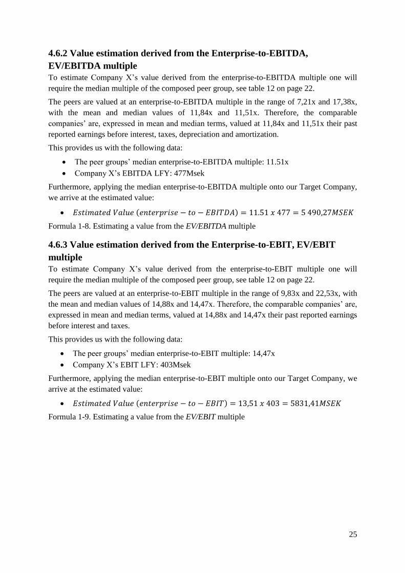
4.6.2 Value estimation derived from the Enterprise-to-EBITDA,

EV/EBITDA multiple

To estimate Company X’s value derived from the enterprise-to-EBITDA multiple one will

require the median multiple of the composed peer group, see table 12 on page 22.

The peers are valued at an enterprise-to-EBITDA multiple in the range of 7,21x and 17,38x,

with the mean and median values of 11,84x and 11,51x. Therefore, the comparable

companies’ are, expressed in mean and median terms, valued at 11,84x and 11,51x their past

reported earnings before interest, taxes, depreciation and amortization.


The peer groups’ median enterprise-to-EBITDA multiple: 11.51x

Company X’s EBITDA LFY: 477Msek

Furthermore, applying the median enterprise-to-EBITDA multiple onto our Target Company,

we arrive at the estimated value:

𝐸𝑠𝑡𝑖𝑚𝑎𝑡𝑒𝑑 𝑉𝑎𝑙𝑢𝑒 (𝑒𝑛𝑡𝑒𝑟𝑝𝑟𝑖𝑠𝑒 − 𝑡𝑜 − 𝐸𝐵𝐼𝑇𝐷𝐴) = 11.51 𝑥 477 = 5 490,27𝑀𝑆𝐸𝐾

Formula 1-8. Estimating a value from the EV/EBITDA multiple

4.6.3 Value estimation derived from the Enterprise-to-EBIT, EV/EBIT

multiple

To estimate Company X’s value derived from the enterprise-to-EBIT multiple one will

require the median multiple of the composed peer group, see table 12 on page 22.

The peers are valued at an enterprise-to-EBIT multiple in the range of 9,83x and 22,53x, with

the mean and median values of 14,88x and 14,47x. Therefore, the comparable companies’ are,

expressed in mean and median terms, valued at 14,88x and 14,47x their past reported earnings

before interest and taxes.


The peer groups’ median enterprise-to-EBIT multiple: 14,47x

Company X’s EBIT LFY: 403Msek

Furthermore, applying the median enterprise-to-EBIT multiple onto our Target Company, we

arrive at the estimated value:

𝐸𝑠𝑡𝑖𝑚𝑎𝑡𝑒𝑑 𝑉𝑎𝑙𝑢𝑒 (𝑒𝑛𝑡𝑒𝑟𝑝𝑟𝑖𝑠𝑒 − 𝑡𝑜 − 𝐸𝐵𝐼𝑇) = 13,51 𝑥 403 = 5831,41𝑀𝑆𝐸𝐾

Formula 1-9. Estimating a value from the EV/EBIT multiple

26

4.6.4 Summary of the traditionally estimated values

Have in consideration that these value estimations are how a traditional comparable company

valuation is applied on substantiated data; however, an analyst often adjusts the multiple,

considering specific risks, by “rule of thumb” and previous market experiences, hence,

arriving at different value estimations.

The estimations received from deriving the three different multiples range between

5 460Msek and 5 831Msek.

Generally, one would add an additional marginal error to this estimation, more on this in the

following chapter.

The three mentioned estimations are plotted in a football-field accordingly.

Msek

6000

5900

5948

5800

5831

5700

5714

5600

5600

5500

5569

5490

5400

5460

5380

5300

5351

5200

5100

5000

P/E

EV/EBITDA

EV/EBIT

Figure 3. Football-field of estimated values derived by their respective multiples including a

high- and low marginal error of 2%

Furthermore, according to the theory of traditional comparable company valuation, the next

step is to perform a mean value of the three estimations, thus, arriving at the estimation:

𝐸𝑠𝑡𝑖𝑚𝑎𝑡𝑒𝑑 𝑉𝑎𝑙𝑢𝑒 (𝑡𝑟𝑎𝑑𝑖𝑡𝑖𝑜𝑛𝑎𝑙 𝐶𝐶𝑉) = ((𝑃/𝐸 + 𝐸𝑉/𝐸𝐵𝐼𝑇𝐷𝐴 + 𝐸𝑉/𝐸𝐵𝐼𝑇)) ⁄

3 = 5 594𝑀𝑆𝐸𝐾

Formula 1-10. Estimating a mean value from the three multiples

27

4.7 The Alternative Comparable Company Valuation According to the alternative comparable company valuation method, in addition to the

traditional comparable company valuation method, one will want to make additional

adjustments to the multiples, thus, instead of using the median value of the multiples to

perform value estimation, one will derive the ‘enhanced’ value multiples from the respective

value drivers, i.e. the percentage expected compounded growth ratios. To determine whether

the relationship between the multiple and its value driver correlate or not the analyst further

looks at observed R Square from the simple linear regression line.

4.7.1 Value estimation derived from the price-to-earnings, P/E multiple

To estimate Company X’s value derived from the price-to-earnings multiple’s value driver

one will require the percentage expected compounded growth rate in earnings, see table 13 on

page 23.

Furthermore, compounding the expected futuristic growth rate in earnings, looking at three

years forward, counted from the fiscal year, results in a value driver of 8,13%, that is, 8.13x.

Hence, creating a scatter plot with the comparable companies’ multiples as y variables and the

respective expected growth rates as the x variables results in the following plot:

Figure 4. P/E with expected diluted earnings growth LFY+1 to FY+3

The simple linear regression equation:

𝑌 = 115,62𝑥 + 7,2208

The equation represents the relationship between the variables y and x, that is, the relationship

between the multiples and the value drivers. To properly understand this equation, recall

chapter 3.5, simple linear regression. The arrows added into the scatter plot represent

Company X’s value driver, 8,13%, here, used to derive the enhanced multiple, thus, finding

its intersection in the linear regression line and thereby deriving its adjusted price-to-earnings-

multiple.

28

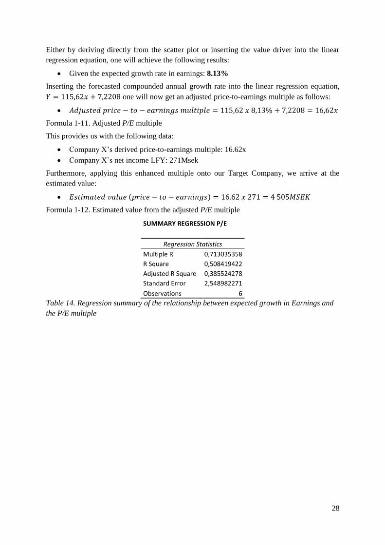
Either by deriving directly from the scatter plot or inserting the value driver into the linear

regression equation, one will achieve the following results:

Given the expected growth rate in earnings: 8.13%

Inserting the forecasted compounded annual growth rate into the linear regression equation,

𝑌 = 115,62𝑥 + 7,2208 one will now get an adjusted price-to-earnings multiple as follows:

𝐴𝑑𝑗𝑢𝑠𝑡𝑒𝑑 𝑝𝑟𝑖𝑐𝑒 − 𝑡𝑜 − 𝑒𝑎𝑟𝑛𝑖𝑛𝑔𝑠 𝑚𝑢𝑙𝑡𝑖𝑝𝑙𝑒 = 115,62 𝑥 8,13% + 7,2208 = 16,62𝑥

Formula 1-11. Adjusted P/E multiple


Company X’s derived price-to-earnings multiple: 16.62x

Company X’s net income LFY: 271Msek

Furthermore, applying this enhanced multiple onto our Target Company, we arrive at the

estimated value:

𝐸𝑠𝑡𝑖𝑚𝑎𝑡𝑒𝑑 𝑣𝑎𝑙𝑢𝑒 (𝑝𝑟𝑖𝑐𝑒 − 𝑡𝑜 − 𝑒𝑎𝑟𝑛𝑖𝑛𝑔𝑠) = 16.62 𝑥 271 = 4 505𝑀𝑆𝐸𝐾

Formula 1-12. Estimated value from the adjusted P/E multiple

SUMMARY REGRESSION P/E

Regression Statistics

Multiple R 0,713035358

R Square 0,508419422

Adjusted R Square 0,385524278

Standard Error 2,548982271

Observations 6

Table 14. Regression summary of the relationship between expected growth in Earnings and

the P/E multiple

29

4.7.2 Value estimation derived from the enterprise-to-EBITDA,

EV/EBITDA multiple

To estimate Company X’s value derived from the enterprise-to-EBITDA multiple’s value

driver one will require the percentage expected compounded growth rate in earnings before

interest, taxes, depreciation and amortization, see table 13 on page 23.

Furthermore, compounding the expected futuristic growth rate in EBITDA, looking at three

years forward, counted from the fiscal year, results in a value driver of 6,31%, that is, 6.31x.

Hence, creating a scatter plot with the comparable companies’ multiples as y variable and the

respective expected growth rates as the x variable results in the following plot:

Figure 5. EV/EBITDA with expected diluted EBITDA growth LFY+1 to FY+3The simple

linear regression equation:

𝑌 = 52,533𝑥 + 6,2229


between the multiples and the value drivers. The arrows added into the scatter plot represent


its intersection in the linear regression line and thereby deriving its adjusted enterprise-to-

EBITDA multiple.



Given the expected growth rate in EBITDA: 6,31%


𝑌 = 52,533𝑥 + 6,2229 one will now get an adjusted enterprise-to-EBITDA multiple as

follows:

𝐴𝑑𝑗𝑢𝑠𝑡𝑒𝑑 𝑒𝑛𝑡𝑒𝑟𝑝𝑟𝑖𝑠𝑒 − 𝑡𝑜 − 𝐸𝐵𝐼𝑇𝐷𝐴 𝑚𝑢𝑙𝑡𝑖𝑝𝑙𝑒 = 52,533 𝑥 6,31% + 6,2229 =

9.54𝑥

Formula 1-13. Adjusted EV/EBITDA multiple

30


Company X’s derived enterprise-to-EBITDA multiple: 9.54x

Company X’s EBITDA LFY: 477Msek


estimated value:

𝐸𝑠𝑡𝑖𝑚𝑎𝑡𝑒𝑑 𝑣𝑎𝑙𝑢𝑒 (𝑒𝑛𝑡𝑒𝑟𝑝𝑟𝑖𝑠𝑒 − 𝑡𝑜 − 𝐸𝐵𝐼𝑇𝐷𝐴) = 9.54 𝑥 477 = 4 551𝑀𝑆𝐸𝐾

Formula 1-14. Estimated value from the adjusted EV/EBITDA multiple

SUMMARY REGRESSION EV/EBITDA



R Square 0,640253815



Observations 6

Table 14. Regression summary of the relationship between expected growth in EBITDA and

the EV/EBITDA multiple

31

4.7.3 Value estimation derived from the enterprise-to-EBIT, EV/EBIT

multiple

To estimate Company X’s value derived from the enterprise-to-EBIT multiple’s value driver

one will require the percentage expected compounded growth rate in earnings before interest

and taxes, see table 13 on page 23.

Furthermore, compounding the expected futuristic growth rate in EBIT, looking at three years

forward, counted from the fiscal year, results in a value driver of 9,01%, that is, 9.01x.

Hence, creating a scatter plot with the comparable companies’ multiples as y variables and the

respective expected growth rates as the x variables results in the following plot:

Figure 6. EV/EBIT with expected diluted EBIT growth LFY+1 to FY+3

The simple linear regression equation:

𝑌 = 107,1𝑥 + 1,5766


between the multiples and the value drivers. The arrows added into the scatter plot represent


its intersection in the linear regression line and thereby deriving its adjusted enterprise-to-

EBIT multiple.



Given the expected growth rate in EBITDA: 9,01%


𝑌 = 107,1𝑥 + 1,5766 one will now get an adjusted enterprise-to-EBIT multiple as follows:

𝐴𝑑𝑗𝑢𝑠𝑡𝑒𝑑 𝑒𝑛𝑡𝑒𝑟𝑝𝑟𝑖𝑠𝑒 − 𝑡𝑜 − 𝐸𝐵𝐼𝑇 𝑚𝑢𝑙𝑡𝑖𝑝𝑙𝑒 = 107,1 𝑥 9,01% + 1,5766 = 11.23𝑥

Formula 1-15. Adjusted EV/EBIT multiple


Company X’s derived enterprise-to-EBIT multiple: 11.23x

Company X’s EBIT LFY: 403Msek

32


estimated value:

𝐸𝑠𝑡𝑖𝑚𝑎𝑡𝑒𝑑 𝑣𝑎𝑙𝑢𝑒 (𝑒𝑛𝑡𝑒𝑟𝑝𝑟𝑖𝑠𝑒 − 𝑡𝑜 − 𝐸𝐵𝐼𝑇) = 11.23 𝑥 403 = 4 526𝑀𝑆𝐸𝐾

Formula 1-16. Estimated value from the adjusted EV/EBIT multiple

SUMMARY REGRESSION EV/EBIT



R Square 0,602299253



Observations 6

Table 15. Regression summary of the relationship between expected growth in EBIT and the

EV/EBIT multiple

33

2.7.4 Summary of the alternative estimated values

The estimations received from deriving the three different multiples range between 4

505Msek and 4 551Msek.

Generally, one would add an additional marginal error to this estimation, more on this in the

following chapter.

The three mentioned estimations are plotted in a football-field accordingly.

Msek

5000

4900

4800

4700

4600

4595

4662

4616

4500

4505

4551

4526

4400

4414

4459

4435

4300

4200

4100

4000

P/E

EV/EBITDA

EV/EBIT

Figure 7. Football-field of estimated values derived by their respective multiples including a

high- and low marginal error of 2%

Furthermore, according to the alternative valuation method, one could either pick one of the

estimated values, since they are rather alike, or perform a mean value of the three estimations;

a mean value arrives at the estimation:

𝐸𝑠𝑡𝑖𝑚𝑎𝑡𝑒𝑑 𝑉𝑎𝑙𝑢𝑒 (𝑎𝑙𝑡𝑒𝑟𝑛𝑎𝑡𝑖𝑣𝑒 𝐶𝐶𝑉) = ((𝑃/𝐸 + 𝐸𝑉/𝐸𝐵𝐼𝑇𝐷𝐴 + 𝐸𝑉/𝐸𝐵𝐼𝑇)) ⁄

3 = 4 527𝑀𝑆𝐸𝐾

Formula 1-17. Estimating a mean value from the three adjusted multiples

The coefficient of determination 𝑅2 varies from 0,5084 to 0,6023 in the three estimations,

recall chapter 3.5.2, hence, interpreting this data and its context is challenging, however,

similar studies show 𝑅2 values close to the ones received, which indicates that there is no

specific need to investigate this further (Frost, 2014).

34

4.8 Comparing the outcome of the two approaches

To be able to draw any conclusions of which approach that resulted in the “best” or most

precise result in the given scenario, the estimations have been presented in a column chart,

compared with the real enterprise value of the fiscal year, since The Target Company is an

already listed company the enterprise value could be found using Bloomberg:

Figure 7. The value estimations received from the traditional- and alternative method,

including the real Enterprise Value of The Target Company year 2015

The alternative approach clearly had more precision in this scenario, hence, outperformed the

traditional approach.

Have in consideration that this is nothing but a sample of one (n=1) and only shows the result

of one valuation made with two different approaches in one given scenario.

To be able to analyze a possible relationship between the composed peer group and its

outcome depending on the two approaches one sample is not enough; therefore, the valuation

process was performed on 6 additional companies in the same manner as the case study.

35

4.9 Applying the two approaches on six additional companies The valuation process was performed on 6 additional companies, resulting in 3 multiple

estimations per approach per company, thus, in total, 36 valuations. The median value of the 3

estimations of each approach was conducted. The results were plotted into a figure, together

with The Target Company, where the orange dot represents a valuation performed with the

alternative approach and the red dot represents a valuation performed with the traditional

approach. The pieces of the pie represent the respective peer. The closer the dot is to the inner

circle, the more precise the outcome was, hence, not being aligned with the inner circle

indicates an over- or under valuation, the further away from the inner circle – the more the

valuation differed from the real value of the company.

Figure 9. Value estimations received from the traditional- and alternative method, performed

on The Target Company and 6 additional companies.

Note that all valuations were made with the same composed peer group, which may affect the

outcome. The results ruled in favor of the alternative valuation method in most valuations,

note that these valuations are prior to adjustments made according to rule of thumb and

personal experience. However, Peer 5 and Peer 10 showed a better valuation given the

traditional approach; this outcome will be further analyzed in the following chapter.

36

5. Analysis

Looking at company valuation in general, one could state that, the valuation is only as good as

the figures that go into it. Having this said, seeing that the process of composing a peer group

plays a significant part in the comparable company valuation methods, the valuation is

therefore only as good as the peer group selected. The composing of the peer group is

described in the theory chapter, where it is stated that the comparable companies must have

similar characteristics to The Target Company. The selection is made of listed companies,

operating in same or similar industries and regions with similar business models and macro-

economic factors. The number of selected peers is however not as extensive, what is

important is how good of a fit they are to The Target Company. The traditional comparable

company valuation method derives the multiple by extracting a mean or median multiple from

the peer group, it is therefore essential that the peer group has very similar, almost exact,

value drivers, in order to arrive at a correct value estimation. Looking at the alternative

method, it is not as essential that the value drivers are very similar; on the contrary, what is of

interest is to capture the relation of the multiples and their respective value driver, since the

adjusted multiples are derived from their correlation. In theory, it should be easier to find

suitable peers to the traditional valuation method if The Target Company operates in a mature

industry since there should be an easy-to-find suitable peer group with very similar value

drivers.

Looking at the figures 4, 5 and 6, one can clearly see that a higher value driver results in a

higher multiple, hence, looking at the upwards sloping simple linear regression line. This

logical reasoning is substantiated by the fact that an investor would pay a higher multiple for a

higher value driver. From an investors’ perspective, one would of course be willing to pay a

higher price for a chance to get a higher return on invested capital.

However, exceptions may occur. Some companies in the graph have very similar value

drivers but trade at different multiples. The reason is that investors require a higher (or lower)

discount rate, due to the fact that different companies have different risks or sufficient

competitive advantages (See chapter 3. Risk). An example of such competitive advantages

could be a market leading product where the entry barriers are high, or, when the company is

a strong market and/or industry leader.

As mentioned in the theory chapter, analysts may make adjustments on the derived multiples

when using the traditional comparable company valuation method; these adjustments are

often made according to “rule of thumb” and personal experience. These adjustments are

based on risks, most often risks such as specific company risks and small company premiums

which have been described in the theory chapter. The alternative company valuation method

can also conduct risk adjustments by adjusting the simple linear regression line downwards or

upwards depending on the peer groups’ risks. However, having risk in consideration, the risk

adjustments conducted would be applied to both valuation methods, hence resulting in similar

risk adjustments, therefore not being essential to this study. In addition, the risk adjustments

preformed in the alternative valuation method are easier to substantiate and therefore easier to

explain rather than adjusting the multiple based on “rule of thumb” and personal experience.

37

The Target Company is a listed company which means that we can benchmark the results

with current market data. We decided on using a listed company for this exact reason, to be

able to validate the results from the different approaches to conclude which approach results

in the most accurate valuation in this scenario given, hence, answer the framed question.

To be able to validate the results given from the case study, we look at multiples for The

Target Company, at the end of year 2015, which we extracted from Bloomberg Terminal.

38

6. Conclusion

The purpose of the thesis was to compare two different approaches and define in what

scenarios they were most applicable.

As stated in the analysis, both approaches to the comparable company valuation method are

highly dependent on the selected peer group. Composing an excellent peer group is therefore

essential for arriving at a correct estimation for The Target Company. However, every

company is different, hence, the task of composing a proper peer group is characterized by an

uncertainty and subjectivity.

With the results provided in in the case study one could draw the conclusion that the

traditional valuation method is favorable if there is a sufficient number of peers to choose

amongst. Providing the analyst with a perfectly composed peer group where the median or

mean multiple actually can resemble The Target Company´s multiple. The traditional

comparable company valuation method is therefore ideal when the target company operates in

a mature industry where a significant number of peers share similar business cycles, risks,

macro-economic factors, and value drivers.

The alternative comparable company valuation method is advantageous when the analyst has

to broaden the peer group in order to derive a correctly estimated value of The Target

Company. The mean or median multiple for a peer group would not resemble the correct

multiple if The Target Company operates in an immature market with a scarce number of

peers with significant differences in company specific risks, market share and value drivers. It

is therefore more important to capture the correlation of what multiple an investor is willing

to pay for a specific value driver and then derive the value of The Target Company from that

analysis. However, the regression equation has shown an R-square that varies from 50 % to

60 %, hence, showing that there is a significance between the multiple and value driver, but it

also indicates that there are other variables at play. The case study provided evidence that

there are companies that have similar value drivers but trade at different multiples indicating

that company specific risks, or a small stock premium significantly affects the multiple. There

may also be additional factors that drive the multiple which cannot be proven in the case

study that was conducted in this thesis.

39

Criticism of own thesis This thesis circulated around a case study regarding The Target Company relative to its peer

group. In order to conduct a valuation using the comparable company valuation method, one

has to make two major decisions that are based on uncertainty and subjectivity. These two

decisions consist of composing a peer group and estimating each company future estimated

value driver. We did not conduct any projections regarding the growth rates in any value

driver but the data provided on Bloomberg consists of projected futuristic data based on

historical performance by each company. No one can see into the future and all projections

based on historical data are uncertain and subjective. The peer group was composed by us and

we followed the guidelines that are described in the theory chapter. However, when

composing a peer group one looks for companies with similar value drivers and the value

drivers consists of futuristic data based on historical performance which means that the

selection of the peer group, to some extent, is based on uncertain and subjective data.

The simple linear regression lines are done with six observations and the simple linear

regression line does not meet all criterions to statistically prove that there is a relationship

between the variables, meaning that predicting the Y-variable with a given X-variable is not

highly reliable. This limitation might have influenced the results in the alternative comparable

company valuation method. The valuation results and conclusions are to be approached with

caution.

This thesis is part of the final course in the Real Estate and Finance program at KTH and the

thesis has to be completed in three months. Due to the short time frame, in which this thesis

had to be completed, we were not able to produce a large sample of valuations. Therefore, the

results and conclusions should be approached with caution.

The original purpose with this thesis was to compare the alternative comparable company

valuation method with the traditional one, to arrive at a conclusion of which approach was

superior. However, as the research took pace we noticed that the traditional valuation method,

in some given scenarios was favorable and other scenarios were in favor of the alternative

valuation method. When we interpreted the results, we noticed that they were superior in

different scenarios, mainly depending on how the peer group was composed. In addition to

this, the question framed was rephrased, in order to pursue a more interesting and useful

purpose.

Further studies To get a clear understanding for the approaches and when they are best used, we suggest that

additional and more extensive studies should be conducted with a larger sample size. Also,

further studies should include extensive research about additional value drivers that influence

the multiples.

40

Bibliography

ABB ltd, 2015. Annual Report, s.l.: s.n.

Addtech AB, 2015. Annual Report, s.l.: s.n.

Alfa Laval AB, 2015. Annual Report, s.l.: s.n.

Alford, A., 1992. The effect of a set of comparable firms on the accuracy of the price-

earnings valuation method, s.l.: J. Account. Res..

Amihud, Y. & Mendelson, 1986. Asset pricing and the bid ask spread. Journal of Financial

Economics, Volume 17, pp. 223-249.

Autoliv Inc. , 2015. Annual Report, s.l.: s.n.

Banz & W, R., 1981. The Relationship between Return and Market Value of Common

Stocks. Journal of Financial Economics, Volume 9, pp. 3-18.

Barker & Richard, G., 1999. European Accounting Review. In: The role of dividends in

valuation models used by analysts and fund managers. s.l.:s.n., pp. 195-218.

Barker & Richard, G., 1999. The role of dividends in valuation models used by. In: European

Accounting Review. s.l.:Routledge Taylor & francis Group, pp. 195-218.

Beckmann, 2003. ZEW Financiall Market Survey, s.l.: ZEW Finanz markt rephrt.

Bergling, L., 2014. Värdering av ett företag som verkar inom en turbulent bransch, Karlstad:

Karlstads Universitet.

Bernstrom, 2014. Valuation: The market approach. s.l.:Wiley.

Bhojraj, Charles, M. & Lee, C., 2002. Who Is My Peer? A Valuation-Based Approach to the

Selection of Comparable Firms. Journal of Accounting Research, Volume 40, pp. 407-439.

Bhojraj, L. D. T. N., 2003. International Valuation Using Smart, s.l.: s.n.

Bis, 2007. Small cap Premium: Does liquidity Hold Water, New York: New York University.

Bloomberg, 2015. Bloomberg. [Online]

[Accessed 06 05 2016].

Capinski & Patena, 2009. Company Valuation - Value, Structure, Risk, s.l.: AGH University

of Science and Technology.

Cooper & Cordeiro, 2008. Optimal Equity Valuation Using Multiples: The Number of

Comparable Firms, s.l.: Research Gate.

Dowdy, Eardon & Chilk, 2004. Statistics for Research. 3 ed. s.l.:John Wiley & Sons.

Fagerhult AB, 2015. Annual Report, s.l.: s.n.

Farquhar, 2012. Case Study Research for Business. s.l.:SAGE Publications Ltd.

Fernandez, 2001. Valuation using multiples, s.l.: IESE Business School.

Frost, J., 2014. Minitab.com. [Online]

Available at: http://blog.minitab.com/blog/adventures-in-statistics/how-high-should-r-

41

squared-be-in-regression-analysis

[Accessed 25 05 2016].

Haldex AB, 2015. Annual Report, s.l.: s.n.

Harbula, 2009. Valuation Multiples: Accuracy and Drivers – Evidence from the European

Stock Market, s.l.: Business Valuation Review, Vol. 28.

Healy & Palpu, 2000. Business Analysis Valuation: Using Financial Statements. 5 ed.

s.l.:Text & Cases.

Henschke, Carsten & Homburg, 2009. Equity Valuation USing Multiples: Controlling for

Differences Between Firms. SSRN Electronic Journal, pp. 10-11.

Hickman, K. & Petry, G., 1990. A Comparison of Stock Price Predictions Using Court

Accepted Formulas, s.l.: Financial Management (summer).

Holton, 2004. Defining Risk. Financial Analyst Journal, Volume 60, pp. 19-25.

Hussey, R., 1999. Discounted Cash flow. In: mac Millan business masters. s.l.:s.n., pp. 265-

273.

Hussey, R. H., n.d. Discounted Cash flow. In: mac Millan business masters. s.l.:s.n., pp. 265-

273.

Höst, Regnell & Runeson, 2006. Att genomföra examensarbete. s.l.:Studentlitteratur.

Israel, T., 2011. The Generous Helping of Company-Specific Risk That May Already Be

Included in Your Size Premium. Business valuation Uppdate, Volume 16, pp. 1-7.

James, R., Hichner & Vogt, P. J., 2005. Cost of capital controversies: It’s time to look behind

the curtain. In: Shannon Pratts Business Valuation. s.l.:s.n., p. Part 3.

Kathman, D., 1998. Are small-cap stocks finally bouncing back?. Stock analyst Journal.

Koller, Goedhart, M. & Wessels, M., 2016. Valuation: Measuring and Managing the value of

compnies. 5th ed. Chicago: McKinsey Company inc.

Liu, Nissim & Tohmas, J., 2002. Equity Valuation Using Multiples. Journal of Accounting

Research, Volume 40, pp. 135-172.

Martins, 2011. International Journal of Law and Management, s.l.: Managerial Law.

Meinhart, T. J., 2008. Estimating a company specific risk premium in the Cost of Capital, s.l.:

Unit Valuation Insights.

Meitner, 2006. The Market Approach to Comparable Company Valuation. s.l.:ZEW

Economic Studies.

Nibe Industrier AB, 2015. Annual Report, s.l.: s.n.

OEM International AB, 2015. Annual Report, s.l.: s.n.

Rutterford, 2004. From dividend yield to discounted cash flow: a. In: Accounting, Business &

Financial History. s.l.:Routledge Taylor & Francis Group, pp. 1-36.

Schmidlin, 2014. The Art of Company Valuation and Financial Statement Analysis: A Value

Investor’s Guide. s.l.:Wiley.

42

Schmidlin, 2014. The Art of Company Valuation and Financial Statement Analysis: A Value

Investor's Guide with Real-life Case Studies. s.l.:Wiley.

Schreiner & Spremann, 2007. Multiples and Their Valuation Accuracy in European Equity

Markets, s.l.: University of St. Gallen.

Sehgal & Pandey, 1981. EQUITY VALUATION USING PRICE MULTIPLES:. ASIAN

ACADEMY of, Volume 6, pp. 89-108.

Simkiss, et al., n.d. Simple Linear Regression - Research methods II. Oxford journal, p.

chapter 2 page2.

SKF AB, 2015. Annual Report, s.l.: s.n.

Suozzo, Cooper, Sutherland & Deng, 2001. Valuation Multiples: A Primer, s.l.: UBS

Warburg.

Tatar, F., 2016. [Interview] (26 04 2016).

The Target Company, 2015. Annual Report, s.l.: s.n.

Weber, M. & Wüstemann, J., 2004. s.l.: s.n.

Xano Industri AB, 2015. Annual Report, s.l.: s.n.

Zarowin, 1990. Size, Seasonality and Stock Market Overreaction. Journal of Financial and

Quantitative Analysis, Volume 25, pp. 113-125.

43

TRITA-FOB-BoF-KANDIDAT-2016:57

www.kth.se

http://www.kth.se/

Documents

Evaluating comparable company valuation967424/FULLTEXT01.pdf · 2016-09-08 · management when allocating money for clients (Barker & Richard, 1999). Corporate valuation is therefore