Evaluating automobile fuel/propulsion system …cushman/courses/engs171/EvalAutoFuel.pdf · ﬁnal evaluation of the alternatives compared to a conventional gasoline-fueled spark

Evaluating automobile fuel/propulsion system technologies

Heather L. MacLeana,*, Lester B. Laveb

aDepartment of Civil Engineering, University of Toronto, 35 St George Street, Toronto, Canada M5S 1A4bGraduate School of Industrial Administration, Carnegie Mellon University, Tech and Frew Sts,

Pittsburgh, PA 15213-3890, USA

Received 1 March 2002; accepted 9 September 2002

Abstract

We examine the life cycle implications of a wide range of fuels and propulsion systems that could power cars and light trucks

in the US and Canada over the next two to three decades ((1) reformulated gasoline and diesel, (2) compressed natural gas, (3)

methanol and ethanol, (4) liquid petroleum gas, (5) liquefied natural gas, (6) Fischer–Tropsch liquids from natural gas, (7)

hydrogen, and (8) electricity; (a) spark ignition port injection engines, (b) spark ignition direct injection engines, (c)

compression ignition engines, (d) electric motors with battery power, (e) hybrid electric propulsion options, and (f) fuel cells).

We review recent studies to evaluate the environmental, performance, and cost characteristics of fuel/propulsion technology

combinations that are currently available or will be available in the next few decades. Only options that could power a

significant proportion of the personal transportation fleet are investigated.

Contradictions among the goals of customers, manufacturers, and society have led society to assert control through extensive

regulation of fuel composition, vehicle emissions, and fuel economy. Changes in social goals, fuel-engine-emissions

technologies, fuel availability, and customer desires require a rethinking of current regulations as well as the design of vehicles

and fuels that will appeal to consumers over the next decades.

The almost 250 million light-duty vehicles (LDV; cars and light trucks) in the US and Canada are responsible for about 14%

of the economic activity in these countries for the year 2002. These vehicles are among our most important personal assets and

liabilities, since they are generally the second most expensive asset we own, costing almost $100 000 over the lifetime of a

vehicle. While an essential part of our lifestyles and economies, in the US, for example, the light-duty fleet is also responsible

for 42 000 highways deaths, and four million injuries each year, consumes almost half of the petroleum used, and causes large

amounts of illness and premature death due to the emissions of air pollutants (e.g. nitrogen oxides, carbon monoxide,

hydrocarbons and particles).

The search for new technologies and fuels has been driven by regulators, not the marketplace. Absent regulation, most

consumers would demand larger, more powerful vehicles, ignoring fuel economy and emissions of pollutants and greenhouse

gases; the vehicles that get more than 35 mpg make up less than 1% of new car sales. Federal regulators require increased

vehicle safety, decreased pollution emissions, and better fuel economy. In addition, California and Canadian regulators are

concerned about lowering greenhouse gas emissions. Many people worry about the US dependence on imported petroleum, and

people in both countries desire a switch from petroleum to a more sustainable fuel.

The fuel-technology combinations and vehicle attributes of concern to drivers and regulators are examined along with our

final evaluation of the alternatives compared to a conventional gasoline-fueled spark ignition port injection automobile.

When the US Congress passed laws intended to increase safety, decrease emissions, and increase fuel economy, they did not

realize that these goals were contradictory. For example, increasing safety requires increasing weight, which lowers fuel

economy; decreasing emissions generally decreases engine efficiency. By spending more money or by reducing the

performance of the vehicle, most of the attributes can be improved without harming others. For example, spending more money

can lighten the vehicle (as with an aluminum frame with greater energy absorbing capacity), improving performance and safety;

a smaller engine can increase fuel economy without diminishing safety or increasing pollution emissions, but performance

0360-1285/03/$ - see front matter q 2003 Elsevier Science Ltd. All rights reserved.

PII: S0 36 0 -1 28 5 (0 2) 00 0 32 -1

Progress in Energy and Combustion Science 29 (2003) 1–69

www.elsevier.com/locate/pecs

* Corresponding author. Tel.: þ1-416-946-5056; fax: þ1-416-978-3674.

E-mail addresses: [email protected] (H.L. MacLean), [email protected] (L.B. Lave).

http://www.elsevier.com/locate/pecs

Nomenclature

AKI anti-knock index

Biodiesel a fuel with characteristics

similar to petroleum diesel

but which is derived from

oils of biological origin (soy-

bean, rapeseed, sunflower).

Some oils can be used with

minimal processing, others

require esterification

Biofuels organic materials, such as

wood, waste, and alcohol

fuels, burned for energy

purposes

Biomass materials that are biological

in origin, such as grasses,

trees, municipal solid waste,

etc.

BPV battery-powered vehicle

CAFE corporate average fuel econ-

omy

CaRFG2 California Phase 2 reformu-

lated gasoline

Cetane colorless, liquid hydrocar-

bon (C16H34) used as a stan-

dard in determining diesel

fuel ignition performance

Cetane number a fuel’s cetane number rep-

resents the ability of a fuel to

ignite and burn under com-

pression

CFC chlorofluorocarbons

CH4 methane

CI compression ignition

CIDI compression ignition, direct

injection

CMU-ET Carnegie Mellon University

equivalent toxicity

CO carbon monoxide

CO2 carbon dioxide

CO2 equiv. carbon dioxide equivalent;

the amount of carbon diox-

ide by weight emitted into

the atmosphere that would

produce the equivalent

radiative forcing as a given

weight of another green-

house gas. Carbon dioxide

equivalents are the product

of the weight of gas being

considered and its global

warming potential.

Compression ratio in an ICE, is the ratio of the

volume of the combustion

space in the cylinder at the

bottom of the piston stroke

to the volume at the top of

the stroke

DI direct injection

E10 mixture of 10% ethanol and

90% gasoline by volume

E85 mixture of 85% ethanol and


EIO-LCA economic input–output life

cycle analysis

EPA US Environmental Protec-

tion Agency

FCV fuel cell vehicle

Fuel cycle the activities associated with

a fuel; from raw material

extraction, through fuel pro-

duction, and finally to end-

use refueling at a refuel

station (also called well-to-

tank)

Gasohol mixture of 10% ethanol and


(also called E10)

GDI gasoline direct injection

GHG greenhouse gas (e.g. carbon

dioxide, methane, nitrous

oxides)

GREET Greenhouse gases, regulated

emissions, and energy use in

transportation, fuel cycle

model developed at Argonne

National Laboratory

GWP global warming potential; an

index used to compare the

relative radiative forcing of

different gases. GWPs are

calculated as the ratio of the

radiative forcing that would

result from the emission of

1 kg of a greenhouse gas to

that from the emission of

1 kg of carbon dioxide over a

fixed time period

HC hydrocarbons

HEV hybrid electric vehicle

ICE internal combustion engine

IO input–output

IPCC intergovernmental panel on

climate change

ISO International Standards

Organization

ISO 14000 International Standards

Organization standard for

H.L. MacLean, L.B. Lave / Progress in Energy and Combustion Science 29 (2003) 1–692

suffers; modern electronics have improved performance, fuel economy, and lowered emissions, but have increased the price of

the vehicle. However, low price and performance are important attributes of a vehicle. To resolve these contradictions,

regulators in the US and Canada need to specify the desired tradeoffs among safety, emissions, fuel economy, and cost, and a

single agency needs to be designated in each country to oversee the tradeoffs among the regulators’ attributes and those desired

by consumers.

implementing an environ-

mental management system

LC life cycle

LCA life cycle assessment

LCC life cycle costs

LCIA life cycle inventory or life

cycle impact analysis

LCI life cycle inventory

LDV light duty vehicles: cars or

light trucks

Lignocellulosic ethanol ethanol derived from fer-

mentation of sugars

extracted from lignocellulo-

sic feedstocks

Lignocellulosic feedstocks woody or herbaceous

materials made up largely

of lignin, cellulose and

hemicellulose

LPG liquid petroleum gas

MJ megajoule

MLCA modified life cycle analysis

(a life cycle assessment

method developed by Ford

Motor Company)

MMBtu million British thermal units

MON motor octane number

MTBE methyl tertiary butyl ether

N2O nitrous oxide

NAAQS national ambient air quality

standard

NEPA National Environmental Pol-

icy Act

NiMH nickel metal hydride

NMOG non-methane organic gases

NHTSA US National Highway

Transportation Safety

Administration

NOx oxides of nitrogen

NREL National Renewable Energy

Laboratory

Octane number expression of the anti-knock

properties of a fuel relative

to that of a standard refer-

ence fuel

O3 ozone

Oxygenate chemical added to gasoline

to increase oxygen content

PEM proton exchange membrane

PM suspended particulate matter

in the air

PM10 particulate matter less than

10 mm in diameter

PNGV partnership for a new gener-

ation of vehicles

POX partial oxidation

RCRA Resource Conservation and

Recovery Act

RFG reformulated gasoline

RON research octane number

QHV lower heating value

RVP Reid vapor pressure

SETAC Society of Environmental

Toxicology and Chemistry

SFC specific fuel consumption

SI spark ignition

SIDI spark ignition, direct injec-

tion (type of engine)

SIPI/SIII spark ignition, port fuel

injection (type of engine)

SMR steam methane reforming

SO2 sulfur dioxide

SULEV super ultra low emissions

vehicle

TRI toxic release inventory

TSP total suspended particulate

matter

ULEV ultra low emissions vehicle

USAMP US Advanced Materials

Partnership

VMT vehicle miles traveled

VOC volatile organic compounds

WTT well-to-tank, the activities

associated with a fuel; from

raw material extraction,

through fuel production,

and finally to end-use refuel-

ing at a refuel station (also

called fuel cycle)

WTW well-to-wheel, the full set of

activities associated with

raw material extraction

through fuel production, dis-

tribution, and use of a fuel in

the vehicle

H.L. MacLean, L.B. Lave / Progress in Energy and Combustion Science 29 (2003) 1–69 3

We discuss methods needed to evaluate the attractiveness of vehicles employing alternative fuels and propulsion systems

including:

1. Predicting the vehicle attributes and tradeoffs among these attributes that consumers will find appealing;

2. assessing current and near term technologies to predict the primary attributes of each fuel and propulsion system as well as

its externalities and secondary effects;

3. applying a life cycle assessment approach;

4. completing a benefit–cost analysis to quantify the net social benefit of each alternative system;

5. assessing the comparative advantages of centralized command and control regulation versus the use of market incentives;

6. characterizing and quantifying uncertainty.

An especially important feature of the analysis is ensuring that vehicles to be compared are similar on the basis of size, safety,

acceleration, range, fuel economy, emissions and other vehicle attributes. Since it is nearly impossible to find two vehicles that

are identical, we use the criterion of asking whether consumers (and regulators) consider them to be comparable. Comparability

has proven to be a difficult task for analysts. No one has managed a fully satisfactory method for adjustment, although some

have made progress. Absurd comparisons, such as comparing the fuel economy of a Metro to that of an Expedition, have not

been made because of the good sense of analysts. However, steps should be taken to achieve further progress in developing

methods to address this issue.

Comparing fuels and propulsion systems require a comprehensive, quantitative, life cycle approach to the analysis. It must be

more encompassing than ‘well-to-wheels’ analysis. Well-to-wheels is comprised of two components, the ‘well-to-tank’ (all

activities involved in producing the fuel) and ‘tank-to-wheel’ (the operation/driving of the vehicle). The analyses must include

the extraction of all raw materials, fuel production, infrastructure requirements, component manufacture, vehicle manufacture,

use, and end-of-life phases of the vehicle. Focusing on a portion of the system can be misleading. The analysis must be

quantitative and include the array of environmental discharges, as well as life cycle cost information, since each fuel and

propulsion system has its comparative advantages. Comparing systems requires knowing how much better each alternative is

with respect to some dimensions and how much worse it is with respect to others. Since focusing on a single stage or attribute of

a system can be misleading, e.g. only tailpipe emissions, we explore the life cycle implications of each fuel and propulsion

technology. For example, the California Air Resources Board focused on tailpipe emissions in requiring zero emissions

vehicles, neglecting the other attributes of battery-powered cars, such as other environmental discharges, cost, consumer

acceptance and performance. The necessity of examining the whole life cycle and all the attributes is demonstrated by the fact

that CARB had to rescind its requirement that 2% of new vehicles sold in 1998 and 10% sold in 2003 be zero emissions

vehicles.

No one fuel/propulsion system dominates the others on all the dimensions in Table 8. This means that society must

decide which attributes are more important, as well as the tradeoffs among attributes. For example, higher manufacturing

cost could be offset by lower fuel costs over the life of the vehicle. Changes in social goals, technology, fuel options,

customer desires, and public policy since 1970 have changed vehicle design, fuel production, manufacturing plants, and

infrastructure. In particular, gasoline or diesel in an internal combustion engine (ICE) is currently the cheapest system

and is likely to continue to be the cheapest system through 2020. These vehicles will continue to evolve with

improvements in performance, safety, fuel economy, and lower pollution emissions. However, if society desires a more

sustainable system or one that emits significantly less greenhouse gases, consumers will have to pay more for an

alternative fuel or propulsion system.

We review a dozen life cycle studies that have examined LDV, comparing different fuels and/or propulsion systems.

The studies are summarized in Tables 4 and 5. The studies vary in the fuel/propulsion options they consider, the

environmental burdens they report, and the assumptions they employ, making it difficult to compare results. However, all

of the studies include the ‘well-to-tank’ and ‘tank-to-wheel’ activities and the majority of the studies include a measure

of efficiency and greenhouse gas emissions associated with these activities. We limit our comparison to these activities

and measures. The life cycle studies match most closely for the well-to-tank portion and for conventional fossil fuels. See

Table 6 for a summary of the ranges of efficiency and greenhouse gas emissions reported in the studies for the well-to-

tank portion for the various options. For the well-to-tank portion for the production of electricity, renewable fuels, and

hydrogen, differing fuel production pathways are most important. Due to the range of different production options for

these fuels (as well as other issues such as study assumptions), results are much more variable. In addition, there is less

experience with producing these fuels, resulting in more uncertainty. It is important to distinguish between total and fossil

energy required for production when comparing efficiencies among the fuels. Petroleum-based fuels have the highest

efficiency for the well-to-tank portion when total energy is considered. However, if only fossil energy is considered,

biomass-based fuels such as ethanol become more attractive.


The tank-to-wheel portions are more difficult to compare. Each study uses its selected vehicle (e.g. conventional

sedans, light-weight sedans, pickup trucks); many present assumptions regarding the vehicle efficiencies. However, the

studies do not generally report the range of assumptions or test conditions.

The well-to-wheel results (the sum of the well-to-tank and tank-to-wheel activities) of the studies are still more difficult

to compare. The baseline vehicle (with a few exceptions) is a current gasoline fueled ICE port fuel injection vehicle; it

combines an efficient well-to-tank portion with a relatively inefficient tank-to-wheel portion. A direct injection diesel

vehicle is considerably more efficient and therefore results in lower emissions of carbon dioxide even though the carbon

content in the diesel is higher than that in gasoline. Fuel cell vehicles have a high theoretical efficiency but generally a

low efficiency well-to-tank portion, which offsets some of the vehicle efficiency benefits.

Table 7 shows the ranges of values reported in the life cycle studies for the well-to-wheel greenhouse gas emissions.

All of the fossil fuel options result in emissions of large amounts of greenhouse gases. Ethanol and hydrogen have the

potential to reduce greenhouse gas emissions significantly. However, this is highly dependent on the pathways for ethanol

and hydrogen production, especially the amount of fossil fuel inputs during production. Some of the hydrogen options

result in higher greenhouse gas emissions than those of a gasoline ICE vehicle. Results for hybrid electric vehicles

(HEVs) are dependent on the efficiency improvements over conventional vehicles that are assumed.

As noted above, Table 8 summarizes our best judgment as to how each fuel/propulsion system combination would be

evaluated on each attribute desired by consumers or society. No one system beats the alternatives on all dimensions. The

most desirable system is defined by the properties that the evaluator thinks are most important.

Despite the many difficulties and complexities, there are some broad conclusions regarding LDV for the next two to

three decades. The vehicle options likely to be competitive during the next two decades are those using improved ICEs,

including HEVs burning ‘clean’ gasoline or diesel. An extensive infrastructure has been developed to locate, extract,

transport, refine, and retail gasoline and diesel. Any alternative to petroleum would require a new infrastructure with

attendant disruption and costs running to trillions of dollars. The current infrastructure is a major reason for continuing to

use gasoline and diesel fuels.

Absent a breakthrough in electrochemistry, battery-powered vehicles will remain expensive and have an unattractive

range. The failure to produce a breakthrough despite considerable research does not give much hope that vastly superior,

inexpensive batteries will be produced within our time frame.

Fuel cell propulsion systems are unlikely to be competitive before 2020, if they are ever competitive. Although, fuel

cells have high theoretical efficiencies, and do not need a tailpipe and therefore have vehicle emissions benefits over

conventional vehicles, generating the hydrogen and getting it to the vehicle requires large amounts of energy. The current

well-to-wheel analyses show that using a liquid fuel and onboard reforming produces a system inferior to gasoline

powered ICEs on the basis of efficiency and environmental discharges. Storage of the hydrogen onboard the vehicle is

another challenge.

Fischer–Tropsch liquids from natural gas and ethanol from biomass may become widespread. The Fischer–Tropsch liquids

will penetrate if there are large amounts of stranded natural gas selling for very low prices at the same time that petroleum is

expensive or extremely low sulfur is required in diesel fuel. Ethanol could become the dominant fuel if energy independence,

sustainability, or very low carbon dioxide emissions become important—or if petroleum prices double.

Absent major technology breakthroughs, a doubling of petroleum prices, or stringent regulation of fuel economy or

greenhouse gas emissions, the 2030 LDV will be powered by a gasoline ICE. The continuing progress in increasing engine

efficiency, lowering emissions, and supplying inexpensive gasoline makes it extremely difficult for any of the alternative fuels

or propulsion technologies to displace the gasoline (diesel) fueled ICE.

This conclusion should not be interpreted as one of despair or pessimism. Rather, the progress in improving the ICE and

providing gasoline/diesel at low price has obviated the need for alternative technologies. Many of the technologies that we

examine, such as cellulosic ethanol or Fishcher–Tropsch fuels from natural gas or HEVs are attractive. If there were no further

progress in improving the gasoline/diesel fuel ICE or the fuel became more expensive, one or more of these options would take

over the market. Thus, the fact that the current fuel and technology is so hard to displace means that society is getting what it

wants at low cost.

Extensive progress has been made by analysts in examining the life cycles of a range of fuels and propulsion systems for

personal transportation vehicles. The most important contribution of these methods and studies is getting decision-makers to

focus on the important attributes and to avoid looking only at one aspect of the fuel cycle or propulsion system or at only one

media for environmental burdens. The current state of knowledge should avoid the recurrence of the fiasco of requiring battery-

powered cars on the grounds that they are good for the environment and will appeal to consumers.

q 2003 Elsevier Science Ltd. All rights reserved.

Keywords: Fuel/propulsion system; Greenhouse gas; Global warming; Life cycle analysis; Life cycle assessment; Alternative fuels


Contents

1. Introduction: importance of motor vehicles . . . . . . . . . . . . . . . . . . . . . . . . . . . . . . . . . . . . . . . . . . . . 7

1.1. Key issues . . . . . . . . . . . . . . . . . . . . . . . . . . . . . . . . . . . . . . . . . . . . . . . . . . . . . . . . . . . . . . . . 8

1.2. Inherent contradictions/tradeoffs in light-duty vehicles. . . . . . . . . . . . . . . . . . . . . . . . . . . . . . . . 8

2. Relevant attributes for evaluating alternative fuel/propulsion systems . . . . . . . . . . . . . . . . . . . . . . . . . 9

2.1. Environmental . . . . . . . . . . . . . . . . . . . . . . . . . . . . . . . . . . . . . . . . . . . . . . . . . . . . . . . . . . . . . 9

2.1.1. Near term: local air pollution . . . . . . . . . . . . . . . . . . . . . . . . . . . . . . . . . . . . . . . . . . . . 10

2.1.2. Toxic air pollutants . . . . . . . . . . . . . . . . . . . . . . . . . . . . . . . . . . . . . . . . . . . . . . . . . . . 11

2.1.3. Environmental: long term, climate change/global warming. . . . . . . . . . . . . . . . . . . . . . . 11

2.2. Sustainability . . . . . . . . . . . . . . . . . . . . . . . . . . . . . . . . . . . . . . . . . . . . . . . . . . . . . . . . . . . . . . 12

2.3. Vehicle attributes . . . . . . . . . . . . . . . . . . . . . . . . . . . . . . . . . . . . . . . . . . . . . . . . . . . . . . . . . . . 12

2.4. Costs . . . . . . . . . . . . . . . . . . . . . . . . . . . . . . . . . . . . . . . . . . . . . . . . . . . . . . . . . . . . . . . . . . . . 13

2.5. Other social issues . . . . . . . . . . . . . . . . . . . . . . . . . . . . . . . . . . . . . . . . . . . . . . . . . . . . . . . . . . 13

2.5.1. Energy independence . . . . . . . . . . . . . . . . . . . . . . . . . . . . . . . . . . . . . . . . . . . . . . . . . . 13

2.5.2. Safety . . . . . . . . . . . . . . . . . . . . . . . . . . . . . . . . . . . . . . . . . . . . . . . . . . . . . . . . . . . . . 14

2.6. Additional issues . . . . . . . . . . . . . . . . . . . . . . . . . . . . . . . . . . . . . . . . . . . . . . . . . . . . . . . . . . . 14

3. Policy analysis methods . . . . . . . . . . . . . . . . . . . . . . . . . . . . . . . . . . . . . . . . . . . . . . . . . . . . . . . . . . 15

3.1. Predicting and influencing market reactions. . . . . . . . . . . . . . . . . . . . . . . . . . . . . . . . . . . . . . . . 15

3.2. Technology assessment . . . . . . . . . . . . . . . . . . . . . . . . . . . . . . . . . . . . . . . . . . . . . . . . . . . . . . 15

3.3. Benefit–cost analysis: valuing the environment and human and ecological health . . . . . . . . . . . . 16

3.4. Market-based tools for achieving social goals . . . . . . . . . . . . . . . . . . . . . . . . . . . . . . . . . . . . . . 17

3.5. Treating and managing uncertainty . . . . . . . . . . . . . . . . . . . . . . . . . . . . . . . . . . . . . . . . . . . . . . 18

3.6. Life cycle assessment . . . . . . . . . . . . . . . . . . . . . . . . . . . . . . . . . . . . . . . . . . . . . . . . . . . . . . . . 19

3.7. Information needed to evaluate alternative fuel/vehicle life cycle inventory studies . . . . . . . . . . . 20

3.8. Importance of ‘vehicle comparability’ in comparative analyses of alternative fuel/vehicle systems 20

4. Attributes of fuel and propulsion system options: technical issues . . . . . . . . . . . . . . . . . . . . . . . . . . . . 24

4.1. Fuels . . . . . . . . . . . . . . . . . . . . . . . . . . . . . . . . . . . . . . . . . . . . . . . . . . . . . . . . . . . . . . . . . . . . 24

4.1.1. Motor gasolines . . . . . . . . . . . . . . . . . . . . . . . . . . . . . . . . . . . . . . . . . . . . . . . . . . . . . . 25

4.1.2. Reformulated gasolines. . . . . . . . . . . . . . . . . . . . . . . . . . . . . . . . . . . . . . . . . . . . . . . . . 26

4.1.3. Diesel fuels . . . . . . . . . . . . . . . . . . . . . . . . . . . . . . . . . . . . . . . . . . . . . . . . . . . . . . . . . 27

4.1.4. Compressed natural gas . . . . . . . . . . . . . . . . . . . . . . . . . . . . . . . . . . . . . . . . . . . . . . . . 28

4.1.5. Alcohols . . . . . . . . . . . . . . . . . . . . . . . . . . . . . . . . . . . . . . . . . . . . . . . . . . . . . . . . . . . 28

4.1.6. Hydrogen. . . . . . . . . . . . . . . . . . . . . . . . . . . . . . . . . . . . . . . . . . . . . . . . . . . . . . . . . . . 29

4.1.7. Liquid petroleum gas . . . . . . . . . . . . . . . . . . . . . . . . . . . . . . . . . . . . . . . . . . . . . . . . . . 30

4.1.8. Liquefied natural gas . . . . . . . . . . . . . . . . . . . . . . . . . . . . . . . . . . . . . . . . . . . . . . . . . . 30

4.1.9. Electricity . . . . . . . . . . . . . . . . . . . . . . . . . . . . . . . . . . . . . . . . . . . . . . . . . . . . . . . . . . 30

4.2. Fuel attributes . . . . . . . . . . . . . . . . . . . . . . . . . . . . . . . . . . . . . . . . . . . . . . . . . . . . . . . . . . . . . 30

4.3. Propulsion systems. . . . . . . . . . . . . . . . . . . . . . . . . . . . . . . . . . . . . . . . . . . . . . . . . . . . . . . . . . 31

4.3.1. Spark ignition port injection engines . . . . . . . . . . . . . . . . . . . . . . . . . . . . . . . . . . . . . . . 31

4.3.2. Spark ignition direct injection engines . . . . . . . . . . . . . . . . . . . . . . . . . . . . . . . . . . . . . . 31

4.3.3. Compression ignition engines . . . . . . . . . . . . . . . . . . . . . . . . . . . . . . . . . . . . . . . . . . . . 31

4.3.4. Electric motor with battery power . . . . . . . . . . . . . . . . . . . . . . . . . . . . . . . . . . . . . . . . . 32

4.3.5. Hybrid electric vehicles . . . . . . . . . . . . . . . . . . . . . . . . . . . . . . . . . . . . . . . . . . . . . . . . 32

4.3.6. Fuel cells . . . . . . . . . . . . . . . . . . . . . . . . . . . . . . . . . . . . . . . . . . . . . . . . . . . . . . . . . . . 32

4.4. Fuel/propulsion system combinations . . . . . . . . . . . . . . . . . . . . . . . . . . . . . . . . . . . . . . . . . . . . 33

5. Attributes of fuel and propulsion systems: social issues . . . . . . . . . . . . . . . . . . . . . . . . . . . . . . . . . . . 33

5.1. Modeling alternative fuel vehicles. . . . . . . . . . . . . . . . . . . . . . . . . . . . . . . . . . . . . . . . . . . . . . . 34

5.2. Vehicle emissions control. . . . . . . . . . . . . . . . . . . . . . . . . . . . . . . . . . . . . . . . . . . . . . . . . . . . . 34

5.2.1. Control issues for alternative fuels . . . . . . . . . . . . . . . . . . . . . . . . . . . . . . . . . . . . . . . . 36

5.2.2. Emissions estimates in life cycle inventory studies. . . . . . . . . . . . . . . . . . . . . . . . . . . . . 36

6. Automobile life cycle assessment . . . . . . . . . . . . . . . . . . . . . . . . . . . . . . . . . . . . . . . . . . . . . . . . . . . 37

6.1. Abbreviated LCA methods . . . . . . . . . . . . . . . . . . . . . . . . . . . . . . . . . . . . . . . . . . . . . . . . . . . . 37

6.2. Design for environment and LCA . . . . . . . . . . . . . . . . . . . . . . . . . . . . . . . . . . . . . . . . . . . . . . . 37

6.3. LCA methods . . . . . . . . . . . . . . . . . . . . . . . . . . . . . . . . . . . . . . . . . . . . . . . . . . . . . . . . . . . . . 37

6.4. LCA of vehicle components . . . . . . . . . . . . . . . . . . . . . . . . . . . . . . . . . . . . . . . . . . . . . . . . . . . 38


6.5. Life cycle stage . . . . . . . . . . . . . . . . . . . . . . . . . . . . . . . . . . . . . . . . . . . . . . . . . . . . . . . . . . . . 38

6.6. Incorporation of cost issues in LCA . . . . . . . . . . . . . . . . . . . . . . . . . . . . . . . . . . . . . . . . . . . . . 38

6.7. Life cycle assessment of light-duty vehicle options . . . . . . . . . . . . . . . . . . . . . . . . . . . . . . . . . . 38

6.8. LCI of conventional automobiles . . . . . . . . . . . . . . . . . . . . . . . . . . . . . . . . . . . . . . . . . . . . . . . 40

6.9. LCI of alternative vehicle options . . . . . . . . . . . . . . . . . . . . . . . . . . . . . . . . . . . . . . . . . . . . . . . 41

6.10. Evaluation of LCI alternative fuel/propulsion system option LCI studies . . . . . . . . . . . . . . . . . . 42

6.11. Evaluated LCI studies . . . . . . . . . . . . . . . . . . . . . . . . . . . . . . . . . . . . . . . . . . . . . . . . . . . . . . . 43

6.12. Comparison of LCI studies . . . . . . . . . . . . . . . . . . . . . . . . . . . . . . . . . . . . . . . . . . . . . . . . . . . . 46

6.12.1. Fuel cycles (well-to-tank—WTT) . . . . . . . . . . . . . . . . . . . . . . . . . . . . . . . . . . . . . . . . . 46

6.12.2. Fuel cycles and vehicle operation (well-to-wheel, WTW). . . . . . . . . . . . . . . . . . . . . . . . 53

6.12.3. Summary of LCA studies . . . . . . . . . . . . . . . . . . . . . . . . . . . . . . . . . . . . . . . . . . . . . . . 56

6.12.4. Summary of study results . . . . . . . . . . . . . . . . . . . . . . . . . . . . . . . . . . . . . . . . . . . . . . . 58

7. Overall results . . . . . . . . . . . . . . . . . . . . . . . . . . . . . . . . . . . . . . . . . . . . . . . . . . . . . . . . . . . . . . . . . 60

8. Conclusions . . . . . . . . . . . . . . . . . . . . . . . . . . . . . . . . . . . . . . . . . . . . . . . . . . . . . . . . . . . . . . . . . . . 62

References . . . . . . . . . . . . . . . . . . . . . . . . . . . . . . . . . . . . . . . . . . . . . . . . . . . . . . . . . . . . . . . . . . . . . . . 64

1. Introduction: importance of motor vehicles

The economies of rich nations and the lifestyle of most

of their residents depend on cars and light trucks [light-duty

vehicles (LDV); LDV are gaining the same role in

developing nations. The manufacture, fueling service and

repair, and disposal of LDV consume about 14% of

economic activity in the United States and Canada. These

represent more than 1/7 of total commercial energy use and

total materials use. These vehicles contribute most of the

carbon monoxide (CO), volatile organic compounds (VOC),

and nitrogen oxides (NOx) emitted in cities; counting

discharges of enginebpv coolant, windshield washer fluid,

used motor oil, and gasoline, LDV are responsible for a

considerable amount of water pollution. Transportation

accounts for 30% of total carbon dioxide (CO2) emissions

from fossil fuel combustion in the USA, with just under 2/3

resulting from gasoline consumption in motor vehicles [1].

LDV are also responsible for considerable expenditures and

environmental disruption due to construction and repair of

highways and parking facilities. Finally, in the US, LDV are

responsible for approximately 42 000 deaths and four

million injuries each year [2] as well as the deaths of untold

numbers of rabbits, deer, and other animals.

In 1995, there were about 600 million vehicles world-

wide, almost 80% of them passenger cars [3]. The USA has

210 million LDV, more than one for every licensed driver.

The fleet uses about 130 billion gallons of gasoline to travel

two trillion miles each year [4]. The total expenditures on

purchasing, financing, fueling, insuring, maintaining, and

repairing the LDV is about $65 000 over the lifetime of a

vehicle [5] or almost $1 trillion each year in the US.

Substantial additions to these out-of-pocket costs are the

time lost due to congestion and injuries. One study estimates

that congestion costs Americans $75 billion each year in

delays [6]. The average American will be injured in a

highway crash during her lifetime and about 1% of

Americans will die in a highway crash; the annual social

loss from highway injuries exceeds $200 billion.1

Why do we devote so many resources to LDV? What do

we get for these expenditures? Perhaps, the most important

attributes that we get are freedom, access, and mobility. We

get to go where we want when we want—subject to

congestion, parking availability, vehicle costs, and other

practical limitations. We can transport ourselves, our

families, and our purchases and possessions.

But mobility explains only a small part of the

expenditure. A basic transportation vehicle would provide

mobility at a fraction of current expenditures. Most drivers

insist on comfort, indeed, luxury. A new, high-end vehicle

has leather seats, air conditioning, a sound system costing

more than $1000, Global Positioning System, and elaborate

wireless communication capabilities. Our cars are status

symbols and projections of how we see ourselves. For

example, using a 7000-pound sports utility vehicle (SUV),

with an engine so powerful that it will take the SUV from 0

to 60 mph in 7.9 s, to get one person to his office is going far

beyond basic mobility.

The goal of this paper is to examine the range of fuels

and propulsion systems that have the potential to power

LDV over the next two to three decades with a focus on the

US and Canada. We focus on fuels and propulsion systems

that could have significant market penetration (more than

1%) during this period. This introduction makes it clear that

motor vehicles are important to the economy and lifestyle of

these countries. Importance goes well beyond the direct

consumer expenditures and indirect (support) expenditures,

such as roads, suburbs, oil wells, refineries, and service

stations. They shape the way we live and how we see

1 Using EPAs value for a premature death of $5.3 million, the

42 000 highway fatalities cost society $222 billion each year.

Adding the social loss from the 4 million highway injuries

increases the social loss to about $250 billion per year.


ourselves. Any attempt to change LDV and their use must

overcome formidable barriers.

1.1. Key issues

Technology developments have created several challen-

gers to the gasoline powered, internal combustion engine

(ICE) vehicle. Which of these are attractive? Which are

more attractive than the gasoline powered ICE?

The current LDV has evolved over a century in response

to consumer demands, social regulations, and changing

technology. Short of some wonderful new technology

emerging, the evolving gasoline fueled ICE will continue

to be the choice of consumers and automakers. Even with

regulatory pressure, it is doubtful that any technology would

displace the gasoline fueled ICE—at least not by 2020 or

2030. Perhaps, the only market signal that would make a

new technology more attractive would be a large increase in

gasoline prices. For example, $3 per gallon gasoline would

encourage people to buy diesel or ethanol powered vehicles,

perhaps in conjunction with a hybrid-electric technology. At

$1.50 per gallon, these alternatives have a tiny market share.

The search for new technologies and fuels is driven by

regulators, not the marketplace. Regulators are mandating

increasingly stringent standards for emissions of air

pollutants, the ability to use alternative fuels, and there is

a warning of more stringent fuel economy standards. In

addition to the concern for improving local air quality,

regulators are concerned about lowering GHG emissions,

dependence on imported petroleum, and switching from

petroleum to a more sustainable fuel.

Regulators can penalize, or even prevent automakers

from selling undesirable vehicles or fuel suppliers from

selling undesirable fuels, but it is difficult to force

consumers to buy what regulators consider to be desirable

vehicles and fuels. Consumer appeal could lead to new

propulsion systems or fuels, but consumers are generally

satisfied with what they have now. For consumers to view

new engines and fuels as more desirable, technology would

have to produce superior performance and economy in these

alternatives, or the current fuels would have to be seen as

less desirable due, for example, to high greenhouse gas

emissions. The greatest force for change is the action taken

by government, from providing roads to regulating the

‘spillover’ effects of each alternative. Social goals influence

what products are allowed on the market and how they are

regulated. In the extreme, if highways are so crowded that

vehicles are useless, vehicle sales will decline.

Some of the choices that motorists make have adverse

effects on the health and well being of others. For example,

the emissions from a vehicle pollute the air that others

breathe. If the vehicle is unsafe or driven unsafely, the lives

of other drivers, pedestrians, and others are put at risk. If a

consumer chooses a vehicle that is a profligate user of raw

materials and fuel, the consumer may be using resources

that otherwise would be available to enhance the well-being

of future generations.

The statistics quoted in the introduction indicate that

automobiles pose major risks to our health and well being,

from death and injury in crashes to air pollution. Thus, in

addition to being the most important consumer product and

offering consumers mobility and access, LDV impose large

costs on society, costs that could grow to the point of

negating their value. These safety and environmental

‘externalities’ are not handled by the marketplace. Regu-

lations are required to correct the incentives. Government

actions are also required to enable this technology by, for

example, building roads or banning tetraethyl lead in

gasoline. However, both automakers and regulators need

to recognize the delicate balance between producing a

product that is desired by consumers and having that product

satisfy social goals as well. We examine this balance in

evaluating the range of alternative fuels and propulsion

systems that could power LDV during the next 20–30 years.

Alternative fuels and propulsion systems have the

potential to solve many of the current social problems and

concerns, from air pollution and global warming to other

environmental improvements and sustainability issues. The

advanced technology could help consumers but not

regulators (more powerful, ever larger vehicles), regulators

but not consumers (tiny, ultra fuel-efficient cars), neither

regulators nor consumers (battery-powered vehicles

(BPV)), or both regulators and consumers (modern, high

efficiency, low emissions gasoline powered ICE). There are

tradeoffs. It is not a foregone conclusion that alternative

fuels and propulsion systems will shove aside advanced

gasoline ICE vehicles within 30 years. We lay out the issues,

review the current state of technology, and examine

alternative propulsion systems and fuels to ascertain their

potential for satisfying both consumers and social concerns.

We address issues of consumer appeal, the local and global

effects of emissions, energy use, sustainability, and energy

security. We do not address issues related to congestion and

land use (including highways and parking).

1.2. Inherent contradictions/tradeoffs in light-duty vehicles

When the US Congress passed laws intended to increase

safety, decrease emissions, and increase fuel economy, they

did not realize that these were contradictory. The easiest

way to increase safety increases weight, which decreases

fuel economy. With the increasing market share of light

trucks, the average fuel economy of LDV sold in the US has

declined and is now 24 mpg, the lowest since 1980 [7].

Growing weight disparity costs society due to the increase in

deaths caused by the collision of vehicles of different

weights [8]. Small, light vehicles have high fuel economy

but are less safe in crashes.

By spending more money, most of the attributes can be

improved without harming others. For example, spending

more money can lighten the vehicle (as with an aluminum


frame with greater energy absorbing capacity), improving

performance and safety. However, low price is an important

attribute of a vehicle.

To resolve these contradictions, the US Congress and

Canadian Parliament need to specify the desired tradeoffs

among safety, emissions, fuel economy, and cost. They also

need to designate single agencies in each country to oversee

the tradeoffs among their attributes and those desired by

consumers. Currently, in the US, the Environmental

Protection Agency (EPA) oversees pollution emissions

and fuel economy, while the National Highway Transpor-

tation Safety Administration (NHTSA) oversees auto safety.

Previous work outlining inherent tradeoffs in LDV includes

Refs. [9–11].

Comparing fuels and propulsion systems requires a

comprehensive, quantitative, life cycle (LC) based envir-

onmental/economic analysis with attention to vehicle

comparability. Since it is nearly impossible to find two

vehicles that are identical, we use the criterion of whether

consumers (and regulators) would consider them to be

comparable (Section 3.8). Focusing on a component of the

LC invites mistaken conclusions. The analysis must be

quantitative because each fuel and propulsion system has its

comparative advantages; comparing systems requires know-

ing how much better or worse each alternative is with

respect to the various dimensions.

We have organized this review by contrasting social

issues with the issues that directly affect automobile

manufacturers and drivers. The important gaps between

the goals of society and those of individual manufacturers

and drivers have been a major justification for government

regulation. After examining these social issues, we review

the tools and methods that are required to analyze the issues.

We then examine the fuels currently used to propel the light-

duty fleet and that are likely to play an important role in

propelling the fleet in the next two to three decades. We then

turn our attention to the propulsion systems currently in use

as well as the propulsion systems likely to be competitive

over the next 20–30 years. Having examined the fuels and

propulsion systems separately, we examine combinations of

systems, since the performance of fuels and propulsion

systems interact with each other. A large amount of

attention has been given to analysis of the life cycles of

the fuels, propulsion systems, and the combinations. We

review these studies in some detail. Finally, we present the

conclusions of our analysis. Appendix A reports fuel

terminology and definitions.

2. Relevant attributes for evaluating alternative

fuel/propulsion systems

Evaluating alternative fuel/propulsion system auto-

mobiles is a multiattribute decision problem. As noted in

Section 1, the importance and ubiquity of light duty vehicles

puts them outside the realm of individual decisions. For

example, if an individual once annoys or injures others, that

is an issue to be ignored as unfortunate or as an issue to be

treated by the judicial system. In contrast, any activity that

involves 1/7 of total economic activity, 1/6 of total energy

use, and almost 1/2 of total air pollution emissions requires

social decisions concerning what designs and uses are

acceptable.

Owners and drivers care about the cost to them of the

vehicle, its fuel, and other expenses. They also care about

the safety of people who ride in their vehicle. In contrast,

their vehicle contributes such a tiny proportion to total fuel

and materials use and to environmental discharges, buyers

are much less concerned about these issues. If energy use,

environmental discharges, and some aspects of safety are

important to society, society will have to take steps to

achieve the desired goals. Social actions can take the form of

(a) command and control regulation, such as refusing to

allow vehicles that do not meet the emissions standards to be

sold, (b) charges and fines, such as the gas guzzler tax for

vehicles that get less than 22.5 mpg, (c) programs that allow

greater flexibility to polluters, such as trading NOx

allowances, and (d) programs that get individuals to change

their behavior voluntarily, such as the use of a designated

driver for people going to a party. For additional details, see

Refs. [12,13].

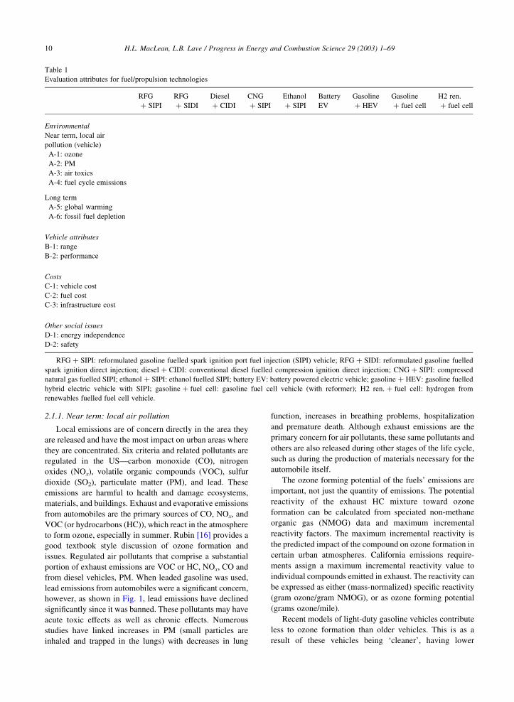
In this section we introduce and discuss the array of

environmental, vehicle, economic and additional social

concerns relevant for evaluating fuel/propulsion system

alternatives. This array of evaluation attributes is the basis

for Table 1, a matrix developed to compare the alternative

fuel/propulsion technologies.

2.1. Environmental

Myriad environmental problems both near and long-term

result from LDV. Perhaps, the most well known is that of air

pollution resulting from the engine exhaust emissions.

Besides this, however, environmental issues include large

volumes of materials and energy used in manufacturing and

servicing automobiles, energy and emissions resulting from

the production of fossil fuels to power them, the fluids used

to lubricate and cool them, as well as wash the windows, and

the materials used at the end of the vehicle’s life. For

example, for the end-of-life stage, approximately 10 million

automobiles are scrapped, disassembled and shredded each

year in the US [14]. Currently, about 75% by weight of an

automobile is recycled, reused, or remanufactured [15]. The

remainder of the automobile is generally sent to a landfill.

This solid waste is referred to as automobile shredder

residue and three to five million tons of it is generated in the

US annually [14]. As aptly noted by Rubin [16], “The

variety of materials used in an automobile and the many

components it contains (a modern automobile has over

20 000 individual parts) mean that any engineering decision

that influences materials choice, shape, or quantity can have

significant environmental consequences.”


2.1.1. Near term: local air pollution

Local emissions are of concern directly in the area they

are released and have the most impact on urban areas where

they are concentrated. Six criteria and related pollutants are

regulated in the US—carbon monoxide (CO), nitrogen

oxides (NOx), volatile organic compounds (VOC), sulfur

dioxide (SO2), particulate matter (PM), and lead. These

emissions are harmful to health and damage ecosystems,

materials, and buildings. Exhaust and evaporative emissions

from automobiles are the primary sources of CO, NOx, and

VOC (or hydrocarbons (HC)), which react in the atmosphere

to form ozone, especially in summer. Rubin [16] provides a

good textbook style discussion of ozone formation and

issues. Regulated air pollutants that comprise a substantial

portion of exhaust emissions are VOC or HC, NOx, CO and

from diesel vehicles, PM. When leaded gasoline was used,

lead emissions from automobiles were a significant concern,

however, as shown in Fig. 1, lead emissions have declined

significantly since it was banned. These pollutants may have

acute toxic effects as well as chronic effects. Numerous

studies have linked increases in PM (small particles are

inhaled and trapped in the lungs) with decreases in lung

function, increases in breathing problems, hospitalization

and premature death. Although exhaust emissions are the

primary concern for air pollutants, these same pollutants and

others are also released during other stages of the life cycle,

such as during the production of materials necessary for the

automobile itself.

The ozone forming potential of the fuels’ emissions are

important, not just the quantity of emissions. The potential

reactivity of the exhaust HC mixture toward ozone

formation can be calculated from speciated non-methane

organic gas (NMOG) data and maximum incremental

reactivity factors. The maximum incremental reactivity is

the predicted impact of the compound on ozone formation in

certain urban atmospheres. California emissions require-

ments assign a maximum incremental reactivity value to

individual compounds emitted in exhaust. The reactivity can

be expressed as either (mass-normalized) specific reactivity

(gram ozone/gram NMOG), or as ozone forming potential

(grams ozone/mile).

Recent models of light-duty gasoline vehicles contribute

less to ozone formation than older vehicles. This is as a

result of these vehicles being ‘cleaner’, having lower

Table 1

Evaluation attributes for fuel/propulsion technologies

RFG

þ SIPI

RFG

þ SIDI

Diesel

þ CIDI

CNG

þ SIPI

Ethanol

þ SIPI

Battery

EV

Gasoline

þ HEV

Gasoline

þ fuel cell

H2 ren.

þ fuel cell

Environmental

Near term, local air

pollution (vehicle)

A-1: ozone

A-2: PM

A-3: air toxics

A-4: fuel cycle emissions

Long term

A-5: global warming

A-6: fossil fuel depletion

Vehicle attributes

B-1: range

B-2: performance

Costs

C-1: vehicle cost

C-2: fuel cost

C-3: infrastructure cost

Other social issues

D-1: energy independence

D-2: safety

RFG þ SIPI: reformulated gasoline fuelled spark ignition port fuel injection (SIPI) vehicle; RFG þ SIDI: reformulated gasoline fuelled

spark ignition direct injection; diesel þ CIDI: conventional diesel fuelled compression ignition direct injection; CNG þ SIPI: compressed

natural gas fuelled SIPI; ethanol þ SIPI: ethanol fuelled SIPI; battery EV: battery powered electric vehicle; gasoline þ HEV: gasoline fuelled

hybrid electric vehicle with SIPI; gasoline þ fuel cell: gasoline fuel cell vehicle (with reformer); H2 ren. þ fuel cell: hydrogen from

renewables fuelled fuel cell vehicle.


tailpipe emissions. In addition, some of the alternative fuels

have lower ozone forming potential than gasoline. For

example, the lower specific reactivity of compressed natural

gas (CNG) exhaust is explained by its composition

(primarily light HCs, either unburned fuel components or

reaction products of methane (CH4) (which have a lower

ozone forming potential than typical HC in gasoline

exhaust)). Gasoline consists of the full range of gasoline

HCs and their combustion products, including more reactive

olefins and aromatics [17].

As shown in Fig. 1, (reproduced from Ref. [18]), there

have been significant reductions in emissions from trans-

portation in the last 20 years, even though vehicle miles

traveled (VMT) has increased substantially. This downward

trend has resulted from the increase in the number of

cleaner, new vehicles satisfying more stringent emission

standards, the retirement of older, higher polluting vehicles,

smog checks, etc.

2.1.2. Toxic air pollutants

Toxic air pollutants (also known as hazardous air

pollutants) are those pollutants that are known or suspected

to cause cancer or other serious health effects, such as

reproductive or neurological problems. Motor vehicles emit

several pollutants that EPA has classified as toxic air

pollutants. These are emitted from all aspects of the vehicle

life cycle; however, the primary focus is on exhaust

emissions from the vehicles themselves. EPA estimates

that mobile sources (e.g. cars, trucks, and buses) are

responsible for releases of air toxics that account for as

much as 50% of all cancers attributed to outdoor sources of

air toxics [19]. For gasoline and diesel LDV, the toxics of

importance are benzene, a known carcinogen, as well as

formaldehyde, acetaldehyde, 1,3-butadiene, and diesel PM,

all of which are classified as probable human carcinogens.

Benzene is a component of gasoline, some of which is

emitted in the exhaust. The other toxics are not present in the

fuel but are produced in the engine or catalyst. The 1990

Clean Air Act requires EPA to regulate air toxics from

motor vehicles in the form of both standards for fuels,

vehicles or both. Since cleaner fuels generally result in

lower emissions of toxics, programs to control air toxics

pollution have focused around changing fuel composition as

well as improvements in vehicle technology and perform-

ance. Some of the alternative fuels are inherently cleaner

than gasoline and diesel, and therefore their use has the

potential to result in reductions of toxics. However, there

may be tradeoffs, with increases of certain toxics (e.g.

aldehydes from alcohol fuels).

2.1.3. Environmental: long term, climate change/global

warming

As recently as a decade ago, climate change was a

relatively obscure concept. It is now a key environmental

policy issue. The 1997 Kyoto Protocol, where international

leaders of major industrialized countries agreed to reduce

their overall emissions of greenhouse gases (GHG) to an

average of 5.2% below 1990 levels by the period 2008–

2012 brought attention to the climate change issue.

However, the Kyoto Protocol has never been ratified, and

therefore countries have only implemented changes where

they have desired to do so. The more recent, 2001

Marrakech climate change talks resulted in a reduced target

of approximately 5% below 1990 levels by 2012. Climate

change is global in scope with potential large-scale

environmental and economic impacts; the potential restric-

tions threaten to impact human behavior and choices. A

significant focus is the potential large-scale shift away from

fossil fuel use.

Gases such as water vapor, CO2, methane (CH4), nitrous

oxide (N2O), and ozone (O3) occur naturally in the earth’s

atmosphere. These gases, along with others including,

halocarbons, and perhalocarbons, are also released into the

atmosphere by human activities. They are called ‘heat

trapping’ or GHG. These GHG create a negative effect when

they trap too much sunlight and block outward radiation.

This is a long-term effect. These GHG have long

atmospheric lifetimes, some remaining for tens or hundreds

of years in the atmosphere and their accumulation over time

is of concern, in that increases in levels of GHG are linked to

increased temperatures [20]. Potential climate risks have

been associated with the increases in GHG. These include

more severe weather patterns, ecosystem change (e.g. loss

of biodiversity), droughts and floods, sea level rise, and

increases in incidence of infectious diseases [20]. In

addition, there may be potential benefits such as longer

growing seasons for agriculture and forestry. GHG gener-

ally do not have short-term effects on human health or

ecology, one exception being ozone which is a main

component of anthropogenic photochemical ‘smog’.

Since road transportation is almost entirely dependent on

fossil fuels, large amounts of GHG are released from LDV.

Carbon dioxide is the substance emitted in the largest

quantity. The transportation sector worldwide is responsible

Fig. 1. National Air Quality Trends Index for Criteria Pollutants:

1975–1997. Source: Table A-9 in US Environmental Protection

Agency [176]. 1975 ¼ 1.0, 1988 ¼ 1.0 for PM-10, CO = carbon

monoxide, NO2 ¼ nitrogen dioxide, PM-10 ¼ particulate matter 10

microns in diameter or smaller.


for about 25–35% of anthropogenic CO2 emissions, most

produced by the combustion of petroleum-based fossil fuels.

For each kg of gasoline used in a car, about 3 kg of CO2 are

released into the atmosphere; therefore, per 100 km, this is

about 20 kg of CO2 being released. The US transportation

sector accounts for about 5% of the CO2 emitted by human

activities worldwide [21]. No other energy use sector in the

US or in another country accounts for a significantly larger

portion of these emissions.

Methane results from activities currently associated with

the automobile LC and potentially would play a more

significant part in an alternative fuel automobile life cycle,

such as CNG production and coal mining, and decomposing

landfill wastes. Nitrous oxide emissions are associated

primarily with the use of nitrogen fertilizers and land use

change, significant sources associated with the production of

ethanol from corn or biomass feedstocks. Car air condi-

tioners used to be a significant source of chlorofluorocar-

bons (CFC) which are halocarbons. CFCs are being phased

out internationally.

Although, the largest quantity of GHG emissions may be

CO2, this does not necessarily indicate that these emissions

have the largest impact on the environment. Since the

different GHG have different atmospheric lifetimes and all

contribute to radiative forcing, the term global warming

potential (GWP) has been devised to weight the various

gases’ contribution to global warming. The term takes into

account the radiative forcing of a gas and its atmospheric

lifetime through using a weighting factor. The GWP of a gas

is defined for a unit mass of the gas relative to a unit mass of

CO2. Carbon dioxide is assigned a weight of one. This

allows analysts to compare combinations of GHG in terms

of an equivalent mass of CO2. For example, the 100-year

GWP based on IPCC values [22] for CH4 is 21 and N2O is

310, indicating that the emission of 1 kg of CH4 contributes

to global warming the same amount as 21 kg of CO2.

Since the light-duty fleet is almost entirely fueled with

fossil-based fuels, its impact on global warming is of

significant concern. Almost all of the carbon in the fuel is

converted to CO2. The important aspects for fossil fueled

vehicles are the carbon content of the fuel and the fuel

economy. Although diesel has a higher carbon content than

gasoline, the higher efficiency of the diesel engine results in

lower vehicle fuel use and therefore lower CO2 emissions

than a ‘comparable’ gasoline engine. Vehicles fueled with

renewable fuels produced sustainably without fossil fuel use

would have no net CO2 emissions. However, there still

remain emissions of non-CO2 GHG. Since CH4 and N2O

have higher GWPs than CO2, these GHG cannot be ignored

in LC studies.

Separating the carbon in fossil fuels and then sequester-

ing it has been proposed as a means of retaining the use of

fossil fuels while ceasing to emit CO2 [23]. This technology

could reduce or eliminate emissions from stationary sources

but would not be feasible for motor vehicles burning fossil

fuels. However, fossil fuels could be transformed into

hydrogen as a motor vehicle fuel, with the carbon

sequestered.

2.2. Sustainability

The Brundtland Commission defined sustainability as

“meeting the needs of the present without compromising

the ability of future generations to meet their needs” [24].

The underlying notion is that current activities should not

impoverish the future.

In the most simple-minded way, sustainability might be

taken to mean that the current generation should not use any

non-renewable resources or rich ores since burning a gallon

of gasoline today means that gasoline will be unavailable to

future generations. Similarly, mining a rich ore body today

means that future generations will be able to mine only

leaner ore bodies. Similarly, anything done to deplete the

soil, such as erosion is unsustainable.

Not only is this simple notion of sustainability unappeal-

ing, it is also too narrow. If, for example, the current

generation develops a technology for mining poor ore bodies

by using no more resources than are required today for rich

ore bodies, the future generations will not be disadvantaged.

Similarly, if the current generation develops alternative

energy sources that are as inexpensive and non-polluting as

extracting and burning petroleum, future generations will

not be disadvantaged by current petroleum use.

Thus, the more general notion of sustainability asks what

opportunities will exist for future generations and whether

their options will be lesser than those of the current

generation. If the answer is that they will have at least as

wide a range of options, then current activities would be

described as sustainable. However, note that the range of

opportunities includes environmental quality and rec-

reational opportunities—which are as likely to be affected

by the growth of population as the depletion of natural

resources.

We do not address sustainability comprehensively in our

evaluation of vehicle options. However, as one component

of sustainability, we consider fossil fuel depletion. In

addition, although we address global warming as a separate

issue in this work due to the current focus on this subject, it

is also a component of sustainability.

2.3. Vehicle attributes

Alternative vehicles,2 which have the potential to make

progress toward achieving social goals, cannot do so in

practice unless consumers choose to purchase them instead

of conventional automobiles. To displace conventional

vehicles, alternative vehicles must be viewed by consumers

as at least equally attractive or ‘comparable’ to these

conventional vehicles. These important attributes are likely

2 Throughout the review we refer to alternative vehicles as any

vehicle options other than gasoline or diesel ICE vehicles.


to include vehicle price, size class, performance, range,

comfort, lifetime, and safety standards. Additionally, it is

necessary that the vehicles be produced in significant

volumes so that supporting infrastructure is available for

refueling and servicing the vehicles. Several of these issues

are included in Table 1 categories other than ‘vehicle

attributes’ (e.g. costs, safety). In our evaluation, for this

section, we concentrate on comparability of vehicle range

and performance, two attributes that vary greatly among

vehicle options and are of significant concern to customers.

The most important aspect of performance (other than

starting) is acceleration, both from a stop and at highway

speeds in order to pass. The time required to accelerate from

0 to 60 mph is a good overall measure of performance.

These performance measures are related to having conven-

ience comparable to that of conventional cars.

Today’s alternative vehicles emphasize a particular

attribute, such as being run by batteries, having improved

fuel economy, utilizing flexible fueling, or being powered

by an alternative fuel. They score well on that dimension,

but tend to be expensive and sacrifice other important

dimensions, such as range, power, or convenience in

fueling. As such, these vehicles are clearly intermediate

steps, and thus are of limited commercial attractiveness. In

some cases, the technology will progress to make the next

generation attractive, as occurred with the direct injection

diesel. In other cases, the technology advances will not be

sufficient to deliver the needed innovations and the

technology will drop from sight, as has occurred with the

battery powered vehicles. The success of the direct injection

diesel puts both automakers and the public on notice that

advanced technology does have attractive contributions to

make. However, there is insufficient data to tell which of the

advanced concepts, if any, will be able to displace the

evolving gasoline powered ICE.

2.4. Costs

The costs of owning and driving a car over its lifetime

include the payments for the car, its fuel, maintenance,

repair, licensing, insurance, and end of life. When a

consumer buys a LDV, the price includes, indirectly, the

cost of extracting the raw materials, transforming them into

materials that go into the vehicle (including fuel and

maintenance items) and the associated transportation and

other manufacturing and distribution costs. Since most

vehicles at the end of their life have a positive value, the

original price of the car also covers the end of life costs.

After purchasing a vehicle, the owner pays for fuel,

maintenance, repair, insurance, and other costs of running

the vehicle. These expenditures cover the costs of extract-

ing, refining, and retailing petroleum products and other

indirect expenses. However, these private costs do not

include most of the costs associated with air and other

pollution, noise, crash related and other injuries, and

congestion. The costs associated with these ‘externalities’

are social costs.

It is important to distinguish between private and social

costs. Automobile manufacturers are motivated to minimize

their private costs in producing a vehicle of a special size

and quality in order to increase their profit. Ordinarily, they

give little or no attention to the social costs. Similarly,

vehicle owners are motivated to minimize their ownership

costs. Regulation is intended to deal with the social costs,

making sure that they are not neglected in the push to

minimize private costs. One approach is to order manu-

facturers to use specified pollution control technology or to

meet discharge standards. Other approaches involve using

market incentives, such as a congestion fee or pollution

emissions fee to internalize the external costs and thus

include them in a company’s efforts to minimize costs [13].

The relatively low costs of current vehicles and fuels

(gasoline/diesel) over their lifetime make it difficult for

alternative fuels and advanced vehicles to compete. In

addition, presently, only gasoline and diesel have the

infrastructure required for fuelling the 1/4 billion North

American vehicles. Fueling a large proportion of LDV with

a different fuel would necessitate significant investment. In

Table 1 we deal with private costs in the ‘costs’ section.

2.5. Other social issues

2.5.1. Energy independence

The 1973 OPEC oil embargo was a shock to the USA and

other oil importing nations. Not only was there a dollar price

to oil, there was a political price as well. Furthermore,

OPEC showed that it could manipulate the dollar price,

leaving importing nations vulnerable to large price increases

and the economic havoc that they could cause.

The USA embarked on an ambitious plan to become

energy self-sufficient. This goal is clearly feasible, since

domestic coal reserves are sufficient to supply enough

energy, although not in the desired liquid form. The program

showed that the USA could become self-sufficient through

the use of oil shale, heavy oil, and conversion of coal to

liquids. However, the economic and environmental cost of

energy independence was high enough to prevent

implementation of the new technologies. The USA

continued to import petroleum and now imports much

more than it did before the embargo. Energy independence

remains a national goal, especially after the Persian Gulf

War and the political instability of many of the OPEC

nations. Energy independence could be pursued through a

number of policies: one is drilling in the Arctic National

Wildlife Reserve, although the USA cannot produce

sufficient petroleum to make up for imports. A second

policy is increasing the fuel economy of new cars; while the

fuel economy almost doubled since 1974, it has been falling

in recent years due to the increasing market share of light

trucks. A third policy is substituting a renewable fuel, such


as ethanol from biomass, for gasoline. We discuss the

second and third policies below.

2.5.2. Safety

The manufacture and use of light duty vehicles is

important to the economy. It is also important in terms of

safety and environment. Tens of thousands of people die

in highway crashes each year in the USA and Canada.

Billions of tons of pollutants are released into the air.

Gasoline is a dangerous liquid in a crash, since it can

explode or ignite. Producing, refining, and transporting

gasoline leads to large environmental discharge of

pollutants. The alternative fuels have implications for

both safety and environment. Some aspects are better and

some are worse, depending on the fuel. We explore some

of these implications.

2.6. Additional issues

Many other social issues are associated with vehicle

choice and use. For example, four-wheel drive vehicles are

used to travel into desert and wilderness areas, sometimes

causing erosion and other damage, disturbing the ecology,

and the enjoyment of hikers and campers. The availability of

low priced, low operating cost vehicles encourages the

dispersion of residences into suburban and rural areas,

leading to highway congestion and the demand for more

highways and parking places. The availability of vehicles

encourages the building of vacation homes and certainly

increases the amount of travel.

We recognize that there are myriad other social issues.

Our failure to discuss them in detail does not indicate that

we view them as unrelated to the central issues in the paper

or as unimportant. Rather, space limitations preclude an

encyclopedic treatment.

Table 1 summarizes the array of environmental, vehicle

attribute, economic, and social concerns for LDV alterna-

tives. The table will be used later in the paper (Section 7) to

summarize the issues for the various fuel/propulsion system

combinations compared to the current gasoline fuel SIPI

engine vehicle.

The above sections introduce the general categories in

Table 1. In the remaining paper, we will introduce and

discuss the issues associated with evaluating each of the

alternative fuel/propulsion options with respect to the

categories. It is not necessary to know much about LDV

to know that there are inherent tradeoffs in any of the

options. For example, fuel economic, lightweight vehicles

benefit global warming and fossil fuel depletion but score

low on safety in the event of a crash. A slightly less apparent

example is that lean burn, direct injection engines are more

fuel-efficient, however, they produce more NOx. How does

society tradeoff safety or tropospheric ozone (related to the

emissions of CO, VOC, and NOx) against using less

petroleum? Society has to choose the dimensions that are

most important.

In some cases, the tradeoffs can be improved by spending

more money on the fuel or propulsion system. For example,

sulfur in the fuel poisons the catalyst. By spending more to

remove sulfur, environmental performance can be

improved. Similarly, turbo charging increases engine

power, allowing a smaller, more fuel economic engine.

However, having low priced fuel and a low priced vehicle

are important. The debates on the level of sulfur in fuel have

been heated. For vehicle fuel economy, automakers work

hard to achieve the fuel economy goal with a vehicle that is

attractive in terms of performance at least cost.

The following example shows the nature of the tradeoffs

as well as the fact that each actor is focusing on his individual

costs. The federal fuel economy legislation gives a 1.2 mpg

fuel economy credit for flexible fuel vehicles (FFV) (those

able to use gasoline or a gasoline-alcohol blend up to 85%

alcohol (E85)). Automakers determined that an FFV should

be optimized for gasoline, not the alternative fuel, since it is

nearly always fueled by gasoline. However, adding the

components that allow flexible fueling increases manufac-

turing cost. Consumers are willing to pay little for an FFV

and so manufacturers cannot recoup their costs. However,

regulators provide an incentive for FFVs: for large SUVs and

some other light trucks, automakers have found that making

the vehicle an FFV is the cheapest way of achieving the

CAFE standards. Thus, automakers make enough FFV to get

their maximum FFV credit. Since the price of ethanol is

higher than the price of gasoline (and it is only available in

very limited supply), drivers find it unattractive to buy the

alternative fuel. Gasohol with 10% ethanol has the largest tax

subsidy per gallon of ethanol; it is the only level of ethanol

that is attractive financially at present [25,26]. Thus,

Congress gave automakers sufficient incentive to produce

FFV but did not give consumers sufficient incentive to buy

the E85 fuel. As a result, almost none of the flexible fuel is

purchased, negating the purpose of the FFV incentives and

the social value of the extra components.

Regulatory agencies have had, and generally continue to

have, narrow goals. The California Air Resources Board has

been concerned primarily with emissions of air pollutants in

California. Greenhouse gas emissions, fuel economy, and

other social issues were not important in their decision to

require a low emissions gasoline and zero emissions or near

zero emissions vehicles. When California groundwater

became contaminated with the gasoline oxygenate methyl

tertiary butyl ether (MTBE), it was the California legis-

lature, not CARB, that ordered the removal of MTBE from

gasoline [27]. Recent legislation in California limiting CO2

emissions will broaden CARBs goals.

Narrow goals are also evidenced in the US government-

industry Partnership for a New Generation of Vehicles [28].

Fuel economy was the primary goal and so they initially

settled on a diesel hybrid, which was more costly to

manufacture and had emissions that could not meet the

requisite standards. Generally, Congress gives each regu-

latory agency a narrow agenda, apparently not realizing that


the agencies’ goals contradict each other [11]. Greater safety

results in a larger, heavier vehicle that gets fewer miles per

gallon. Lower emissions generally result in additional

vehicle cost. Congress and in Canada, the Canadian

Parliament need to resolve these contradictions.

3. Policy analysis methods

In order to get meaningful comparisons among the

vehicle options, a range of tools can be applied. The

underlying issue in each case is the efficiency-advantage of

each technology. For example, how much will reducing the

weight of a car by 10 kg increase fuel economy? How much

could lowering engine power, as measured by an increase in

the 0–60 mph acceleration time, increase fuel economy?

How much more efficient is a direct injection engine

compared to a port injection engine? In Section 4, we

address these technical issues, drawing together the

scientific literature and the judgment of a range of experts

where data are not available.

3.1. Predicting and influencing market reactions

In a market economy, incentives are important. Drivers

want to pay less to fuel their vehicles. Since, ethanol from

corn is more expensive to produce than gasoline, few drivers

would be expected to buy ethanol. However, ethanol

producers receive a federal tax reduction of $0.53 per

gallon and up to $0.40 per gallon in state taxes in some

states. These tax breaks provide a sufficient incentive to

produce large quantities of ethanol from corn, despite its

higher cost of production.

Another example concerns the mix of vehicles produced

and their pricing. The Corporate Average Fuel Economy

(CAFE) standards require automakers to sell small, light

vehicles with small engines in order to sell large, heavy

vehicles with large engines. For example, to achieve a

CAFE of 27.5 mpg, an automaker could sell one vehicle

getting 44 mpg in order to balance a 20 mpg full size car.

Consumers want the latter and are willing to pay high prices

to get them. Some Americans want small, fuel efficient cars,

but CAFE requires automakers to sell more of these cars

than Americans would desire if the price-cost markup were

the same as for large powerful vehicles. As a consequence,

CAFE gives a strong incentive to automakers to boost the

price of large vehicles in order to subsidize the price of small

vehicles so that the average new car sold will attain the

CAFE standard.

Consumer demands, legislation, regulations, and tax

incentives provide a vast network of incentives that

influence the production and sale of LDV. In our analysis,

we try to identify and control for these incentives.

Regulations are perhaps the strongest incentive. For

example, a vehicle model that does not pass the emissions

certification requirements cannot be sold. Automakers have

no choice except to meet these emissions standards. In

contrast, the fuel economy standard offers considerably

greater flexibility. First, the fuel economy of all new

vehicles from a manufacturer is averaged. This averaging

allows some vehicles to have poor fuel economy, as long as

they are balanced by fuel-efficient models. Second, the

legislation even allows manufacturers to accumulate CAFE

credits and carry them forward to future years. Finally, if all

else fails, a manufacturer can pay a fine that is proportional

to the fuel economy shortfall.

3.2. Technology assessment

Evaluating vehicles that have not yet been built is

inherently difficult. Evaluating current vehicles is far easier.

Despite the difficulties, there is no alternative to finding

methods to project the attributes, useful lifetimes, and

manufacturing costs of advanced vehicles. For example, the

spark ignition port injection (SIPI) ICE has been evolving

for more than a century. Although engineers continue to

improve its longevity, power, fuel economy, and emissions,

the improvements are evolutionary. In contrast a direct

injection engine is new and improvements are likely to be

more rapid. The same is true for a hybrid electric vehicle

(HEV) and a fuel cell vehicle (FCV). It makes no sense to

rule out these new technologies because they are not

competitive today. However, a judgment is required as to

how rapidly and to what point these technologies are likely

to advance. Many new technologies, even technologies of

promise, are unable to overtake existing technologies.

Deciding how stringent a regulation should be is

complicated by the fact that the average automobile is

expected to last almost 15 years. Stringent regulations that

make new vehicles more expensive or less attractive to drive

would lengthen the life of existing vehicles, since

consumers would be reluctant to trade them in for more

expensive or less desirable vehicles. This actually occurred

during the 1970s when air pollution standards made new

vehicles less desirable and led consumers to keep old, highly

polluting vehicles [29].

Technology forcing is a type of regulation designed to

force automakers to find and perfect new technology [30,

31]. In the post-World War II period, automakers focused on

power and size, giving relatively little attention to lower

emissions levels, greater fuel economy, or greater safety. If

regulators had simply required automakers to incorporate

the best available emissions control, safety, and fuel

economy technology, little would have been gained.

Instead, regulators promulgated ‘technology forcing’ stan-

dards designed to get automakers to develop new technol-

ogy to meet the regulations. Unfortunately, some of the time

the technology forcing results in expensive vehicles which

consumers do not find attractive. Bresnahan and Yao

estimate that forcing technology for emissions control in

the early 1970s in the US resulted in social losses of tens of


billions of dollars, although eventually automakers were

able to find technology that met the standards.

In the US, Congressional, EPA, and California EPA

technology forcing was effective in lowering vehicles

emissions. This has carried over into Canada. Compared

to 1968 vehicles, current vehicles have reduced their

emissions by 90–95% for CO, NOx, and HC. Lead

emissions have been reduced almost to zero as a result of

banning the fuel additive. In contrast to the success story of

tighter emissions standards and technology forcing, pro-

grams such as inspection and maintenance on vehicles in

service and vehicle retirement programs have been less

successful [32].

In a laboratory setting, many new technologies look

extremely attractive. These technologies can solve one or

more current problems, such as emissions or fuel economy.

However, it is difficult to estimate the cost, reliability, and

other attributes of a new technology in the prototype phase.

It is even more difficult to estimate how people will use the

technology when it is mass-produced and used under real

world conditions. Drivers tend to neglect maintenance and

to push the technology beyond its stated limits. If this abuse

results in danger or extremely high costs result from failure

to maintain the technology precisely as directed, the

technology is unlikely to be attractive in mass production.

It is impossible to anticipate the indirect effects of a new

technology. For example, building automobiles and fueling

them with gasoline eventually resulted in adding tetraethyl

lead to gasoline, the Persian Gulf War, the Exxon Valdez,

and urban ozone; adding air bags led to childrens’ deaths;

building tires of rubber led to fires in piles of discarded tires.

It is difficult to imagine that the developers of automobiles

could foresee the amount of materials and petroleum used,

the amount of environmental discharges, or the vast changes

in cities that the invention caused. People will use a new

technology in ways that please them—which is not

necessarily what the developers intended or desired.

Being able to get a reasonable picture of the implications

of a new technology requires a life cycle assessment (LCA),

an evaluation of the inputs and outputs of a product/process

from the extraction of raw materials to the manufacture of

the product, its use, and its end-of-life. Without this

comprehensive look, analysts can be deceived about the

desirability of a new technology. For example, because the

vehicle itself has no emissions, CARB, General Motors, and

some other automakers saw BPV as the solution to

environmental problems caused by LDV. However, this

limited view failed to take account of the electricity needed

to recharge the batteries or the effects of mining and

smelting heavy metals, making the metals into batteries, and

recycling the batteries. Lave [33] found that if these

batteries were charged with electricity generated from the

national average generation mix, the emissions of NOx and

CO2 would be greater than those of the best comparable

current gasoline powered vehicles being sold in the US.

They also found that mining and smelting battery materials

and making and recycling batteries put enormous quantities

of toxic material into the environment. This LC-based

analysis revealed that BPV, at least with current batteries

and electricity generation, are not better for the environment

than comparable sized conventional vehicles. In Section 5,

we present formal analyses of the LC of various fuels and

propulsion technologies.

In assessing a technology, there are two questions: (1)

Compared to what? (2) Is this technology, on net, desirable?

A technology might be expensive, unreliable, and polluting.

However, if it is better than the current technology, and is

better than other alternatives, it might be substituted for the

current technology. For example, the LDV produced from

1975 to the present have polluted the environment and used

large quantities of fuel. However, each generation of

emissions control has been better than the previous

generation, leading to less undesirable emissions. Unfortu-

nately, there is always the question as to whether, on net,

this technology is desirable. In the late 1970s, most

Americans (and most people in developed nations) decided

that nuclear power was not a net benefit to society. Methyl

tertiary butyl ether (MTBE) is a desirable additive to

gasoline, resulting in lower emissions from some vehicles.

However, gasoline spills have resulted in MTBE contami-

nated groundwater, which led California to ban its use [27,

34]. They decided the use of MTBE did not result in a net

benefit.

3.3. Benefit–cost analysis: valuing the environment

and human and ecological health

Public decisions such as setting emissions or ambient air

quality standards have enormous implications for both the

economy and the environment. Making informed public

policy decisions requires a systematic analysis of their

implications. A number of decision frameworks are used to

assess whether a proposed regulatory action is in the public

interest [11]. The most comprehensive framework is

benefit–cost analysis. This framework has been used by

the Army Corps of Engineers to assess waterway projects

since 1930s. Benefit–cost analysis enumerates the desirable

and undesirable effects of a policy, relates the effects

quantitatively to the degree of control, translates each effect

into dollars, brings each dollar value to current dollars, and

then compares the benefits and costs. For example, the direct

benefits of automobile emissions control include lower

ambient air concentrations of ozone, CO, NOx, and small

suspended particles. The downstream benefits include

reductions in morbidity and mortality and a reduction in

acid precipitation. The direct costs include the cost of the

emissions control devices while the downstream costs

include reductions in power and fuel economy for a given

engine. All these desirable and undesirable effects must be

translated into dollars, the effects over the life of each

vehicle must be discounted to the present, and the benefits

and costs compared. The framework requires a vast amount


of quantitative data as well as difficult judgments such as the

dollar value of improvements in environmental quality (for

example, see EPAs retrospective study of the benefits and

costs of the Clean Air Act, 1970–1990 [35].

When people hear about benefit–cost analysis, they

usually think that putting a dollar value on the effects and

finding the right discount rate, are the most difficult and

complicated. In practice, economists conducting a benefit–

cost analysis are hampered because the goals of the program

are not carefully specified. Not carefully stating the goal of a

program makes it difficult to find the preferred actions, to

run the program efficiently, or to evaluate afterward whether

it accomplished the purpose. A benefit–cost analysis

requires quantification of the effect of each intervention,

e.g. the number of lives that would be saved by putting air

bags in LDV. Generally, the information on the quantitative

relationships is not available or is unreliable.

For goods valued in the marketplace, price provides a

good metric, as long as the market is competitive and the

price is not skewed by a temporary disequilibrium. For some

products, there are important externalities (non-market

effects) associated with the product. For example, prior to

the 1970s, buying a gallon of gasoline included a range of

environmental discharges during drilling, production, trans-

portation, refining, and storage (leaky underground storage

tanks). In the past, the dollar price of gasoline significantly

understated the social costs of that product. As regulations

have lowered these discharges by changing drilling and

production practices, requiring doubled-hulled tankers,

reducing environmental discharges from refineries, and

eliminating leaky underground storage tanks, the price of

gasoline has risen to cover these costs and now comes much

closer to representing the social-environmental costs of the

product.

Goods and services not traded in the marketplace are

more difficult to value. For example, what is the value of

preserving a wilderness area or of non-polluted air? A large

literature comments on the good and bad aspects of

proposals to value these non-market goods [36–38,174,

177]. Values can be estimated by taking the amount that

people spend on travel to see an event, by finding private

goods that are relatively similar to the public good, or by

statistical analyses that disentangle the amount that people

are willing to pay for a house that has a good view, is located

near a lake or other amenity, or is in an area with low air

pollution. While the measures are imperfect, they are clearly

better than ignoring these aspects, since that assumes that

the value of these goods is zero.

Matthews and Lave [39] examined values that four state

public utility commissions along with a number of

researchers have estimated for the social cost of emitting

air pollutants. California, Nevada, New York, and Massa-

chusetts put somewhat different values on CO, CO2, total

suspended particles (TSP), sulfur dioxide (SO2), and NOx,

however, the values fall within a plausible range and are

related to the estimates of these values that come from

the literature on the damage that results from polluted air.

Matthews and Lave [39] analyze the variation-uncertainty

explicitly by considering the full range of values and find

that an explicit analysis of uncertainty is needed when

translating the physical effects into dollar terms. The dollar

values depend on where the air pollutants are emitted

(population in the surrounding area), uncertainty concerning

the health effects of the pollutants, the inherent values

associated with abating urban ozone and other pollution, and

probably on the current ambient air quality. They certainly

depend on the income and environmental attitudes of the

people doing the evaluation. Reflecting these consider-

ations, the dollar values in the four state studies and in the

research literature differ by more than a factor of 10.

The US Environmental Protection Agency [35] has

analyzed the retrospective and prospective benefits and

costs of the 1970 Clean Air Act (and its subsequent

amendments). EPA was faced with all of these issues in

estimating both the benefits and costs from 1970 to 1990 and

from 1990 to 2010. EPA found the greatest scientific support

for health effects of small particles suspended in the air

(PM10) and so almost the entire calculated benefits stem

from these estimated health effects. The economics

literature justifies a high dollar value for the benefit of

preventing premature death ($4.8 million, according to

EPA) and so preventing premature death contributed almost

90% of the benefit of abating air pollution. The benefits of

abating NOx, CO, and VOC were ignored, except in so far as

they led to PM less than 10 mm (PM10).

The EPA analysis all but ignores other categories of

benefits, such as ecology, damages to materials and

visibility and more general benefits of abating air pollution.

EPA was mindful of these categories of benefits, but the

scientific literature provides little basis for estimating the

benefits of abatement. EPA also estimated little or no benefit

from abating hazardous air pollutants because the scientific

literature does not provide an adequate basis for estimation.

See also Ref. [40].

3.4. Market-based tools for achieving social goals

A competitive market is marvelous for producing

cheaply the goods and services that consumers desire. The

pressures to innovate and reduce costs pushes aside attaining

other social goals, goals not explicitly sought by consumers

in the marketplace, such as lowering environmental

discharges. If your competitor lowers production costs by

not worrying about environmental discharges, you will be at

a competitive disadvantage, unless your customers are

willing to pay more for your environmentally benign

product.

These problems were recognized in the 1960s and 1970s;

environmental legislation was passed that created federal

and state regulatory agencies that could set and enforce

discharge and ambient quality standards. Initially, the

standards were explicit and detailed in terms of the specific


abatement technology or the amounts of discharges that

would be allowed from individual point sources. However,

the extent to which pollution can be abated and the cost of

abatement differs across each source. Federal and state

regulatory agencies do not have the data, expertise, or

personnel to set and enforce these detailed standards.

With US Congressional encouragement, EPA tried a

different approach to regulating environmental discharges

[13]. For example, as lead was being phased out of gasoline,

it became evident that refineries had different capabilities of

producing gasoline with the required octane when they

could not boost octane with tetraethyl lead. Rather than

compel all refineries to follow the same phase out schedule,

EPA gave ‘allowances’ to refineries that phased out lead

more quickly than was required. These refineries could sell

the allowances to refineries that were not able to meet the

standards. This more flexible approach gave an incentive to

refineries to clean up more rapidly, stopped the inevitable

complaints from those that could not, and yet met the phase

out schedule. Evaluators concluded that granting this

flexibility helped the program to succeed by having fewer

challenges in the courts and political process and allowing

refineries to adhere to the phase out schedule.

Granting allowances and flexibility for individual

polluters was tried on a much larger scale in the 1990

Clean Air Act [41,42]. Congress instructed EPA to use an

allowance approach to cut SO2 emissions in half from coal

burning electricity generators. The cost of lowering SO2 is

estimated to have decreased by at least 2/3 due to using

allowances to give individual plants flexibility. Allowances

are also being used in abating NOx and VOC.

As noted above, Congress used a flexible approach to

regulate fuel economy, since it allowed automakers to

offset gas-guzzlers with gas-sippers, as long as the average

new car sold by a manufacturer met the fuel economy

standard [8].

Policy analysts and Congress have concluded that

allowing greater flexibility is beneficial, as long as there is

stringent pressure to keep polluters focused on attaining the

goal. The flexibility is especially valuable when it is

combined with market incentives, such as tradable allow-

ances. However, introducing flexibility and market incen-

tives requires polluters and regulators to collect more data

and engage in more record keeping. For example, if plant X

wants to sell 10 000 SO2 allowances, the regulators have to

make sure that they have earned the allowances. If plant Y

buys the allowances, the regulators have to make sure that

the levels of emissions are not greater than the total number

of allowances that they have. This was feasible for SO2

since the emitters were large and could afford continuous

emissions monitoring. The monitoring cost would be too

large for smaller sources, although other approaches might

prove feasible. In particular, it is hard to see how allowance

trading could be applied to individual automobiles.

Continuous monitoring is too expensive and some drivers

might tamper with their engine and control system after

inspection to increase the power of the vehicle. Additional

discussion of regulatory methods can be found in Refs. [13,

42–45].

3.5. Treating and managing uncertainty

Policy analysis and most technology and business

decisions are complicated by the fact that some of the

most important parameters are unknown, or at least

uncertain. Waiting until the uncertainty is resolved means

waiting until many opportunities have passed. While

regulators who act before all the information is collected

and analyzed might regulate the wrong pollutant or set a

standard that is too lenient or too stringent, regulators have

to tradeoff the cost of delaying action against the cost of

setting the wrong standard by acting prematurely. For

example, there has been more than 30 years of controversy

as to the relative importance of the health effects of SO2,

CO, NOx, ozone (O3), and suspended particles. The US EPA

feels reasonably confident that it can quantify the major

health effects of air pollution, using TSP or PM10 as a

surrogate. However, there is considerable uncertainty about

the health effects of each of these individual pollutants.

One way of dealing with uncertainty is to ignore it. When

EPA initially set the national ambient air quality standards,

there was so little data that EPA tended to ignore

uncertainty. One consequence was that when the ozone

standard was revisited in 1977, EPA relaxed the standard

from 80 to 120 ppb.

A second way of treating uncertainty is to conduct a

sensitivity analysis. Often the analyst takes the plausible

range and conducts an analysis to see the implications of

using values from the middle and extremes of this range

[39]. Alternatively, the analyst can try to find ‘critical’

values that make an important difference to the analysis.

Usually implicit in a sensitivity analysis is the assump-

tion that the analyst has no idea of the likelihood that each

outcome is likely to be correct [46]. For example, is the

lowest value extremely unlikely or somewhat unlikely? If

the analysis can put a subjective probability estimate over

the distribution of values, a Monte Carlo analysis can be

conducted. In this analysis the probability density function

of the parameter values can be translated into a probability

density function of outcome values. For example, if there

were a distribution of the effects of PM10 on mortality in

New York City, a Monte Carlo analysis would give the

probability density of the number of deaths on a given day as

a function of the concentration of PM10 and the number of

people exposed to the air pollution. This outcome

distribution gives more information than the sensitivity

analysis. Unfortunately, the distribution is no better than the

analyst’s judgment on the initial probability density

function.

A final way of analyzing uncertainty is to construct a

‘scenario’ or conditional probability analysis [47]. The

scenario assumes that uncertainty is resolved in a particular


way and then examines the implications. The scenario

analysis can be regarded as an exercise in science fiction or

as a rigorous application of conditional probability analysis

that is related to sensitivity analysis and Monte Carlo

simulation.

Even when the best of these analysis tools are

applied, the uncertainty is still likely to be important.

One way of managing the uncertainty is to find strategies

that are robust in the face of the uncertainty. For

example, there might be a regulation that, while not

optimal for any value of the effect of PM10 on mortality,

tends to be good across a wide range of values. Thus, the

analyst needs to search for regulations that are good

across the range of likely uncertain values, rather than

for regulations that have the greatest net benefits for a

particular value. Sources providing details about uncer-

tainty issues include Lave (1994) and Morgan [46].

3.6. Life cycle assessment

Researchers in the US and Europe have developed LCA

methods most extensively. LCA is a systematic tool to

provide information on the environmental impacts of

alternative materials, products, processes and services.

LCA attempts to trace out the major stages and processes

involved over the entire life cycle of a product. In the US,

the Society of Environmental Toxicology and Chemistry

(SETAC) [48] and the US EPA [49–51] led the way in

method development, publishing guidelines for LCA.

Keoleian [52] presents a good overview of the life cycle

design framework developed by USEPA. In Europe, similar

guidelines have been issued by the Nordic Council of

Ministers [53]. These methods utilize process models to

trace the chain of material and energy flows all the way back

to primary extraction.

The International Organization for Standardization (ISO)

has recently published LCA guidelines that fall within their

ISO 14000 series for implementing an environmental

management system. They classify the LCA standards with

other ‘product oriented’ standards, including environmental

labeling. The LCA standards are ISO 14040: Environmental

Management, LCA, Principles and Framework; 14041: Life

Cycle Inventory Analysis; 14042: Life Cycle Impact

Assessment; 14043: Interpretation. These four standards

address the four components of LCA.

Goal definition and scooping. This first component of the

LCA requires defining the purpose and the scope of the

study including boundary definition, establishing the func-

tional unit to be considered (e.g. an automobile with a

lifetime of 150 000 miles), documenting assumptions, study

limitations, and procedures for quality assurance of the

results. Many of the controversies associated with LCA

result from the assumptions made at this stage.

Inventory analysis. This LCA stage is an accounting of

the energy and raw materials use and discharges to all media

over the entire life cycle of the product, material, process,

etc. Information in a life cycle inventory (LCI) includes, for

example, for an automobile, the number of kg of CO2

emissions from the use life cycle stage (the driving of the

vehicle throughout its lifetime).

Impact analysis. ‘Impact analysis in LCA is a

systematic process to identify, characterize, and value,

potential eco-system, human health, and natural resource

impacts associated with the inputs and outputs of a product

or process system’ [50]. To date, this life cycle stage has

not been implemented comprehensively. Sometimes the

results of the inventory analysis have been aggregated into

impact categories such as global warming and ozone

depletion [54,55]. However, most studies have stopped

short of actually characterizing and valuing impacts on

health.

Improvement analysis. This final LCA component is a

systematic evaluation of the needs and opportunities to

reduce the environmental burden associated with the life

cycle of the product. Both quantitative and qualitative

options should be proposed.

LCA of automobiles have focused on inventory analyses.

Several studies have taken steps to present impact measures,

e.g. GWP, weighted toxics, etc. but none have resulted in a

complete impact analysis. Newell [56] presents a LC

method that makes progress in moving beyond inventory

information by calculating social costs through estimating

damage functions. We treat LCA for automobiles more

extensively in Section 6.

Unfortunately, the ‘conventional’ LCA method and the

results of studies utilizing this method have generated much

controversy. Critics have charged that LCA cannot

accomplish what is desired [54,57,58], Field [180]. Con-

troversies over boundary selection, the difficulty that each

industry is dependent directly or indirectly on most others

for inputs resulting in the chain of inputs into a product

expanding exponentially and the presence of circularities

have been some of the difficulties. Analysts have struggled

to obtain detailed and accurate, up to date data for all of the

processes required. As a result, often they have had to draw

narrow boundaries. Differences in the results of analyses of

even simple products such as paper versus polystyrene foam

(plastic) cups [54,59–61] indicate some of these short-

comings. Joshi [62] provides a thorough discussion of

conventional LCA shortcomings.

In 1995, researchers from the Green Design Initiative at

Carnegie Mellon University, Pittsburgh, PA proposed using

economic input–output analysis techniques for overcoming

the boundary problem in conventional LCA [54,62,63]. The

method, called economic input–output life cycle analysis

(EIO-LCA), has evolved into a comprehensive LCI tool

with publicly available data. The model is available free of

charge on the internet [64]. The current version utilizes the

1997 485 sector by 485 sector matrix of the US economy

augmented with an environmental matrix.


3.7. Information needed to evaluate alternative fuel/vehicle

life cycle inventory studies

LCA has long emerged from its exploration phase.

Unfortunately, many analysts continue to act as if they are

the first to face these issues and do not bother to compare

their results to previously published work. Rather, analysts

in the alternative vehicles area need to recognize that the

LCA studies have the same overall goal: evaluate the

attractiveness of alternative fuel/vehicle propulsion systems

for the next 20–30 years. However, it is difficult to

determine overall results from even one study and even

more difficult to compare studies. The majority of studies do

not present sufficient detail to analyze the method and

results thoroughly. In most cases, little economic data are

included and there is little discussion about the differing

levels of development of the technologies and required

infrastructures and how these impact the results that are

reported. To provide valuable information to decision

makers and facilitate study comparison, in our judgment,

all studies should present the following core set of

information.

(i) All options should be clearly specified and time frame

and geographic location of analysis noted. Quantitat-

ive results for fuel cycle and vehicle operation should

be presented clearly. For other life cycle stages

(manufacture, service, end-of-life), at least qualitative

information should be presented, detailing the most

important differences in a particular option from

today’s conventional vehicles and fuels.

(ii) A baseline conventional SIPI gasoline fueled vehicle

should be included as a benchmark. Each vehicle

being analyzed should be characterized by its style,

size class, range, vehicle lifetime, thermodynamic

efficiency and fuel economy (city/highway).

(iii) All alternative vehicle options should be modeled

taking into account comparability from the point of

view of the consumer and regulator (Section 3.8). This

should include at a minimum; performance (accelera-

tion, etc.), range, size class, style, vehicle lifetime,

power to weight ratio, and emissions levels. Where it

is not possible for an option to achieve equivalent

attributes, this should be noted. Thermodynamic

efficiencies and fuel economies (city/highway) of all

vehicles should be reported, along with the level of

development and a quantitative estimate of

uncertainties.

(iv) The studies should include a standard set of GWPs for

weighting the greenhouse gases, a standard lifetime

(200 000 km) and a standard driving cycle for fuel

economy and emissions. Since vehicles are used in

different ways, the study can go on to present a driving

cycle and lifetime that is most relevant for that model.

However, it is important to present a standard scenario

in order to compare the results with other studies.

(v) Each study should present current reformulated gaso-

line (RFG) or diesel as a standard test fuel for

comparison. This standard will provide an anchor

point for comparison with other studies and other

fuels. If the focus is on the well-to-tank (WTT)—fuel

cycle stage, the studies need to define a standard for

reporting that is comparable to the Delucchi or Wang

(GREET) frameworks [65,66]. Additional details

about these frameworks are presented in Section 6.9.

For biofuels, the studies need to specify the yield of

volume of fuel/land area required to produce that fuel

(e.g. gallons/acre) based on the near term situation as

well as assumptions regarding sustainable production

(assumptions regarding little use of fossil fuels

throughout fuel cycle). For all fuels, the study should

present estimates of emissions of regulated pollutants

and toxics, GHG as above from raw materials

extraction, transportation, and carbon sequestration

where applicable.

(vi) Almost all studies have been conducted as if vehicle

prices are irrelevant. Price is certainly not irrelevant to

consumers. Thus, a good study should include

estimates of the cost per vehicle mile (including initial

purchase price, fuel, vehicle service, and fixed costs).

The studies to date suggest that the costs of

conventional ICE options are likely to be similar,

even for those with direct injection engines or fueled

with CNG or cellulosic ethanol. However, the costs

may be greater for electric vehicles.3 For new fuels or

vehicles, the study should contain a description of the

infrastructure changes that are required and estimated

costs.

(vii) When assumptions are being made about future

improvements in technology, such as efficiency of

the ICE or costs of cellulosic ethanol, the study should

be explicit about the nature of the assumptions and, if

possible, their justification.

(viii) Finally, results and associated uncertainties should be

clearly presented.

3.8. Importance of ‘vehicle comparability’ in comparative

analyses of alternative fuel/vehicle systems

Comparability of vehicles can mean that the vehicles

have identical power, size, range, etc. Alternatively, it can

mean that customers (and regulators) find the bundle of

attributes of a vehicle at least equally attractive compared to

the bundle of attributes of alternative vehicles. The latter

criterion for comparability is most useful when it is all but

impossible for the alternative car to deliver the same

attributes as a current gasoline powered car. For example, if

certain drivers do not regard a decrease in range as

important, then the design could be shifted to compromise

3 In this review, we use the term electric vehicles to refer to

battery-powered, hybrid electric and FCVs.


the unimportant attributes in order to score well on the

desired attributes.

For vehicles that consumers do not regard as compar-

able, making analytical adjustments to render them

comparable is difficult, but ignoring differences among

vehicles is perilous. The fuel and vehicle system must be

treated as a system when looking at comparability; the

comparability of individual components is not relevant. A

straightforward, but difficult, method of making vehicles

comparable is to adjust fuel economy for differences in

power, range, and weight. For example, EPAs Hellman [67]

developed a formula for gasoline fueled vehicles to adjust

fuel economy for differences in power. Adjusting for

comparability does not end the difficulty. Some fuel/

propulsion system combinations are better for some

performance goals. For example, batteries are good only

for short range, CNG for low emissions, diesel for high fuel

economy. Battery-powered vehicles (BPV) have an advan-

tage for operating in enclosed spaces or other areas that are

difficult to ventilate.

Current sales of conventional vehicles show that

consumers desire a wide range of designs. Some consumers

desire small sports cars with quick acceleration. Others buy

sport utility vehicles, the larger the better. No vehicle can

meet the requirements of all consumers. However, to be

‘commercial,’ a vehicle has to appeal to enough consumers

so that it meets at least the minimum scale economies in

manufacturing, about 100 000 vehicles per year. To provide

convenient servicing, a vehicle must command at least 1%

of new vehicle sales. Thus, the 100 000 units per year could

be sold in 10 countries to account for manufacturing scale

economics, but the vehicle would not find convenient

servicing.

Up to this point, we have focused primarily on vehicle

comparability. There are related fuel comparability issues

that must be considered. Primary issues include the potential

for large-scale production/availability of the fuel at

reasonable economies of scale. For example, ethanol from

biomass is available at a relatively low cost when the

feedstock is bagasse or other biomass residues. When this

supply is used up and the feedstock costs $45/ton, the costs

rise sharply.

Each fuel must satisfy the baseline availability, technol-

ogy development (proven versus requiring technology

breakthroughs), safety, suitable storage and vehicle use,

and meet fuel regulations. Special attention must be paid to

the attributes of the fuels not currently in large-scale

production and their associated issues. For example, the vast

majority of energy required to produce gasoline is from

fossil fuels, whereas, renewable biofuels have the potential

to be produced without using any fossil fuels and so would

have no net CO2 emissions. Failing to differentiate between

these two sources of energy use would be misleading.

Gasoline and diesel are taxed heavily in Europe and

Japan and taxed moderately in many nations. While the tax

motivates drivers to purchase vehicles with greater fuel

economy and to drive less, it also serves to raise large

revenues for government. Any fuel that assumes a large

share of the market will have to pay its share of taxes. Thus,

the comparison among fuels should be on the basis of

refinery gate cost or of retail price, where each fuel has the

same tax burden. It is misleading to compare the untaxed

price of one fuel to the taxed price of another.

Comparability has proven to be the most difficult task for

analysts. No one has managed a fully satisfactory method

for adjustment, although some have gotten further than

others. The principal reason why absurd comparisons have

not been made, such as comparing the fuel economy of a

tiny Metro to that of an Expedition SUV, is the good sense

of analysts. However, we cannot depend on the good sense

of all future analysts. We review, briefly, the way in which

analysts have adjusted for vehicle comparability in their

analyses.

Analysts have made varying levels of progress in

accounting for equivalency in examining automobile

alternatives. Recently, LCA studies comparing alternative

fuel/vehicle options have devoted more attention to

comparability of the vehicles and fuels they analyze [10,

68–70]. We examine several studies, including these recent

examples as well as earlier works, noting the steps taken into

account for comparability and their impact on the study

results. These studies were completed with a focus on

product planning, sustainability, and environmental

impacts.

Since alternative fuels and advanced vehicles on the road

today and in development are not optimized for perform-

ance, comparisons of these vehicles with the best conven-

tional gasoline ICE vehicles are misleading. The latter have

been refined over a century. To level the playing field

somewhat, many researchers have estimated the potential

efficiencies of various alternative-fueled automobiles [9,

71–74] compared to a baseline gasoline automobile. These

estimates have been generally based on the thermal

efficiency of the alternative fueled vehicle propulsion

system compared to that of a gasoline vehicle for combined

city/highway driving, taking into account the fuel and

engine properties. This is a first step. However, not taking

into account the comparability of the remainder of the

vehicle (e.g. whether diesel vehicles can achieve the stated

efficiency and meet the same emission standard as the

conventional gasoline vehicle or if the CNG vehicle has a

range only half that of the conventional vehicle, or

comparing a 2-seater with a luxury sedan) will lead to

misleading results. The fuel/engine combination must be

placed within the social context of being comparable from

both consumer and regulatory perspectives.

Of all alternative fueled vehicle studies, Delucchi [65,71]

and Wang [66] modeled the most extensive sets of

alternative-fueled passenger cars with production of fuels

from various pathways. The analysts used previous studies

and expert judgment to model the vehicles, primarily through

adjustment of their fuel economies based on estimated


efficiencies compared to a baseline conventional automobile.

Vehicle emissions were based on emissions standards,

vehicle test results, and modeling. In lieu of making an

assumption about vehicle lifetimes, the model results were

presented on a per mile basis. The model results did not state

whether the vehicles were of equivalent size, range, or were

comparable in other performance parameters. The fuels and

corresponding fuel cycles were modeled based on production

data and engineering judgments.

Kreucher [75] is another early study reporting LCA

results for various conventional and alternative fueled

vehicles. He addressed comparability by modeling the

vehicle options from a Ford Escort, assuming 100%

penetration of the particular fuel option and constant vehicle

lifetime. In addition, cost differentials from the baseline

Escort were calculated.

Sullivan [76] held powertrain performance constant in

examining an ICE gasoline engine Taurus and three diesel

(compression ignition ICE) ‘functionally equivalent’

vehicles. Sullivan mentioned the increase in emissions for

the diesel options and the issue of meeting regulatory

standards but did not appear to adjust the vehicle efficiency

to account for emissions treatment required to meet the

standard or to account for the additional costs associated

with reducing the weight of some of the vehicle options.

Brekken [77] developed a method for comparing the

efficiency of competing propulsion technologies and fuels.

To compare vehicles, the authors start with a baseline Ford

Taurus and calculate the total energy required to move a

vehicle from point A to point B, starting with the original

source of the energy. All of the vehicles are also required to

do the same amount of useful work. They also considered

comparability of power to weight ratio and range.

MacLean [68] and Lave [10] accounted for several of the

aspects of comparability that, in their judgment, are highly

valued by consumers and regulators, modeling the vehicles

from a baseline popular conventional gasoline ICE vehicle,

the 1998 Ford Taurus LE sedan. Their studies utilize the

Taurus conventional sedan fueled with unleaded gasoline as

the baseline vehicle. In modeling alternative fuel ICE

vehicle options, the authors held constant, vehicle style and

size class, driving range, lifetime, emissions level (Cali-

fornia Ultra Low Emission Level (ULEV)), and comfort. In

addition, the vehicles were modeled assuming large-scale

penetration of the vehicle/fuel options into the market, and

in estimating efficiency differences from the baseline

vehicle it was assumed that all of the combinations were

optimized for their fuel and met the ULEV emissions

standard. However, the performance of the options has not

been proven, and comparable vehicle attributes, e.g.

acceleration, interior and trunk space, etc. were not held at

the same level as the baseline vehicle. The authors show the

significant impact on vehicle weight (and therefore,

performance) of not holding vehicle range constant

(Fig. 2). The impact is most significant for fuels that have

low energy densities, such as CNG, and, to a lesser extent,

ethanol.

MIT [69] noted that they ‘evaluate in a consistent way

major new vehicle and fuel technologies which have the

potential to reduce significantly the emissions of GHGs’.

The study examined technical characteristics of new

technologies, GHG and other emissions, energy efficiencies,

costs, consumer perceived performance, convenience,

safety, and reliability. The study selected a baseline

average-size (US) passenger car, gasoline fueled with an

ICE and with the evolutionary improvements expected by

the year 2020; the vehicle is assumed not to incur extra costs

other than those necessary to keep up with the market. As in

the GM/Argonne study, the MIT study looked at options that

could be produced and used at a volume great enough to

capture most of the economies of scale. The study assumed

that all vehicles will meet US Federal Tier 2 national

requirements for emissions and accounted for estimated

costs of the emission control system required.

The MIT study reported that ideally, each vehicle

alternative should provide the same acceleration, drivabil-

ity, driving range, refueling ease, interior driver and

passenger space, trunk space and meet applicable safety

and pollutant emission standards. The analysts took steps to

deal with these issues, but remark that only some of them

could be dealt with quantitatively in the study. The attributes

that they held constant among the vehicle options were that

all propulsion system and vehicle combinations were

adjusted to provide the same ratio of maximum power to

total vehicle mass (75 W/kg), driving range of 600 km

(except the BPV), vehicle size was kept relatively constant,

they assumed that the California Low Emission Vehicle

(LEV) II and EPA Tier II emissions standards for 2004–

2008 could be met by improved exhaust gas treatment

technology for the ICE engines and were within reason for

fuel cell systems (noting that the least confidence was placed

on the diesels meeting these standards), and some

consideration of cost differences. Vehicle options were

modeled using computer simulations and assuming the

vehicles go through specified driving cycles. The vehicles

utilized advanced technologies in the propulsion systems

and lightweight materials and reduction of other driving

resistances, aerodynamic drag and rolling resistance. The

BPV were not comparable in range.

A study by General Motors and Argonne National

Laboratory [70] considered comparability with respect to a

number of important issues. First, the authors reported that

the study is limited to fuel/vehicle options having the

potential for large volume penetration in the LDV market

from 2005 to 2010. The mass, and aerodynamic and rolling

resistance coefficients of the vehicles in the study were

based on a conventional gasoline fueled GM Silverado full

size pickup truck. The focus of the study was on the

potential for improving fuel economy (efficiency), while

maintaining the vehicle performance demanded by North

American consumers. The study specified performance


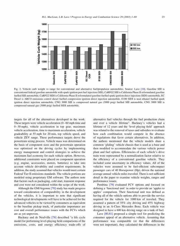
targets for all of the alternatives developed in the work.

These targets were vehicle acceleration (0–60 mph time and

0–30 mph), vehicle acceleration in top gear, maximum

vehicle acceleration, time to maximum acceleration, vehicle

gradeability at 55 mph for 20 min, top vehicle speed, and

vehicle ZEV range. These performance targets drove the

powertrain sizing process. Vehicle mass was determined on

the basis of component sizes and the powertrain operation

was optimized on the driving cycles by implementing

energy management and control strategies to achieve the

maximum fuel economy for each vehicle option. However,

additional constraints were placed on component operation

(e.g. engine, accessories, motors, batteries) to take into

account vehicle drivability and comfort requirements. In

addition, the study assumed that vehicles would meet certain

Federal Tier II emissions standards. The vehicle portions are

modeled using proprietary GM software. The authors note

that factors such as packaging, cold start, transient response

and cost were not considered within the scope of the work.

Although the GM/Argonne [70] study has made progress

toward consideration of comparability in the development

of the vehicles, it is important to note that significant

technological developments will have to be achieved for the

advanced vehicles to be viewed by consumers as equivalent

to the baseline pickup truck, of particular importance are

cost and overall performance issues with the FCVs which

are as yet unproven.

Hackney and de Neufville [78] described “a life cycle

model for performing level-playing field comparisons of the

emissions, costs, and energy efficiency trade-offs of

alternative fuel vehicles through the fuel production chain

and over a vehicle lifetime”. Hackney’s vehicles had a

lifetime of 12 years and the ‘level playing field’ approach

was related to the removal of taxes and subsidies to evaluate

how each combination would compete in the absence

of regulations that favor certain alternatives. In addition,

the authors mentioned that the vehicle models share a

common ‘gliding’ vehicle chassis that is used as a base and

then modified to accommodate the various vehicle power

plant and fuel options. Efficiencies of each vehicle’s drive

train were represented by a normalization factor relative to

the efficiency of a conventional gasoline vehicle. They

included some uncertainty in efficiency values. All of the

vehicles were assumed to be fuel-efficient subcompact

passenger cars of 40 Horsepower (Hp), driven the national

average annual vehicle miles traveled. There is not sufficient

detail in the paper to examine vehicle weights, ranges and

performance issues.

Pembina [79] evaluated FCV options and focused on

defining a ‘functional unit’ in order to provide an ‘apples to

apples’ comparison. Their functional unit was defined as

having all of the vehicle options able to provide the service

required for the vehicle for 1000 km of traveled. They

assumed a pattern of 55% city driving and 45% highway

driving in an A-Class Mercedes Benz. Each vehicle was

designed to have a 600 km driving range on a tank of fuel.

Lave [80,81] proposed a simple tool for predicting the

consumer appeal of an alternative vehicle. Assuming that

performance was comparable (or that the differences

were not important), they calculated the differences in the

Fig. 2. Vehicle curb weight vs range for conventional and alternative fuel/propulsion automobiles. Source: Lave [10], Gasoline SIII is

conventional federal gasoline automobile with spark ignition port fuel injection (SIII), CaRFG2 SIII is California Phase II reformulated gasoline

fuelled SIII automobile, CaRFG2 SIDI is California Phase II reformulated gasoline fuelled spark ignition direct injection (SIDI) automobile, EC

Diesel is ARCO emissions control diesel fuelled compression ignition direct injection automobile, E100 SIDI is neat ethanol fuelled spark

ignition direct injection automobile, CNG 3000 SIII is compressed natural gas (3000 psig) fuelled SIII automobile, CNG 3000 SIII is

compressed natural gas (3000 psig) fuelled SIDI automobile.


costs of owning a conventional (Toyota Corolla) and

alternative (Toyota Prius HEV) vehicle over their

lifetimes. The cost differences included initial purchase

price, fuel, and any differences in service and mainten-

ance. Since the Prius has better fuel economy and lower

emissions of pollutants and GHG, they calculated the

‘breakeven’ price of gasoline ($3.55/gallon), pollution

emissions (11 times the assumed median values from

Ref. [39]), and GHG emissions ($130/ton CO2) that

would equate the lifetime ownership costs of the two

vehicles (assuming the current price premium of $3495

for the Prius over the Corolla). Alternatively, they

calculated the price premium for the HEV that would

equate the lifetime ownership costs and asked whether it

would be possible to manufacture an HEV for this cost

premium. Finally, they asked what characteristics an

advanced vehicle whose size and performance were

comparable to a Corolla would have to have in order

to be attractive to consumers. Suppose an advanced

vehicle used no fuel and had no pollutant or GHG

emissions. How much more than the Corolla could this

vehicle sell for and still have the same lifetime owner-

ship costs? The authors came up with the value of $5540

(assuming a discount rate of 6%). These calculations

illustrate how difficult it is for advanced vehicles to

displace the modern SIPI engine vehicle. Although, HEV

are likely to improve significantly from the initial models

in terms of performance and cost, it appears that, unless

the hybrids offers performance features worth more to the

consumer than those of the conventional vehicle, they are

unlikely to gain a large market share.

More generally, this analysis framework allows an

automaker to evaluate any prospective alternative vehicle

against a conventional vehicle with respect to lifetime costs.

Adjusting for other differences between vehicles is more

difficult. For example, the Toyota Prius is similar to the

Corolla, allowing for relatively straightforward adjustments

to make them reasonably comparable. The Honda Insight

(another HEV) is much smaller and not directly comparable

to other models sold in the USA, making adjustment

difficult. Less costly examples include CNG vehicles and

E85 used in flexibly fueled vehicles. This tool can be used to

calculate the value of an improvement in fuel economy or

lowering of pollution or GHG emissions. While each

fuel/vehicle combination has some advantages and dis-

advantages compared to conventional gasoline vehicles, the

costs and improvements of alternative vehicles are hard to

justify in competition with the best current vehicles. For

new fuels, infrastructure and convenience of fuel supply are

major issues as well.

Predicting the performance of technologies not in large-

scale production and comparing these with those that are is

exceedingly difficult. Even though some of the above noted

studies consider vehicle and fuel comparability to a

reasonable extent, there remains much work to be done in

this area.

4. Attributes of fuel and propulsion system options:

technical issues

This section discusses fuel and propulsion system

options with the potential for large-scale use in the next

two to three decades. We begin by describing the fuel and

propulsion system options individually. This discussion is

necessarily general since specific vehicle attributes (e.g.

efficiency, fuel economy, and performance) depend on the

fuel/propulsion system pair. Thus, following this initial

discussion we focus on specific fuel/propulsion system

combinations. Since there is a broad literature in the area of

characteristics of alternative fuels and propulsion systems,

we provide some introductory material and focus on primary

aspects that differentiate the options but refer readers to

additional sources for more detailed information.

4.1. Fuels

Nearly all motor vehicles today are powered by either

gasoline or diesel. Both fuels are derived from petroleum, a

non-renewable resource. The gasoline and diesel sold today

is not the same as that sold in the 1960s, since regulations

have forced the reformulation of these fuels to improve

environmental performance. These reformulated fuels have

lower sulfur and fewer aromatics; tetra-ethyl lead is banned

throughout the USA and Canada.

In 2000 in the US, 67% of petroleum consumption was

for transportation and the transport sector is 97% dependent

on petroleum [3]. Gasoline and diesel have an enormous

infrastructure that supplies the fuel each year to the US and

Canadian light-duty fleets. These fuels are attractive for

LDV because of their price, availability, ease of use, and

high energy density. However, production, refining, trans-

port and use of these fuels cause local and global

environmental problems. If a substantial portion of the

fleet were to run on an alternative fuel, a large infrastructure

would have to be constructed at enormous cost and

protest [72].

We discuss the characteristics of conventional and

alternative fuels under consideration in the near term for

light-duty transportation, focusing on those most relevant

for assessing their potential for large-scale use. Guibet [82],

Poulton [72], DOE [83], Owen [84], NREL [85], and

Argonne National Laboratory website and publications [14]

are good sources for information about alternative fuels,

their properties, advantages and disadvantages of their use

for personal transportation. Selected properties of the fuels

are shown in Table 2 and described in the following

sections. Fuel property definitions are in Appendix A.

The efficiency of production of a fuel from raw materials

(well-to-tank) is an important attribute. Where little

processing is required, the efficiency is high, e.g. gasoline

from crude oil. Where a great deal of processing is required,

the efficiency is low, e.g. Fischer–Tropsch fuels from coal

or natural gas. For renewable fuels, efficiency of production


is not well defined. It could be defined as the ratio of the

energy in the fuel to the energy in the sunlight that struck the

relevant portion of ground. It seems most useful to estimate

the number of square meters of ground required to propel a

standard vehicle a specified distance.

However, large investments are required to transform

sunlight or biomass into fuel. A LCA is required to calculate

the total materials and energy required for the process. For

example, with a photovoltaic cell, a smaller area of ground

is needed to propel a vehicle a mile than would be needed to

grow the amount of biomass required to produce the ethanol

necessary to propel that vehicle a mile. However, a great

deal more materials, labor, and energy are required to make

the photovoltaic cell than is required to produce the ethanol.

Thus, a full LCA is required to determine which is better.

4.1.1. Motor gasolines

Gasoline is a blend of hydrocarbons with some

contaminants, including sulfur, nitrogen, oxygen and certain

metals. The four major constituent groups of gasoline are

olefins, aromatics, paraffins, and napthenes. These groups

vary in their octane level and reactivity. Petroleum varies in

density, chemical composition, boiling range, etc. For

example, petroleum from the Persian Gulf tends to be

high in aromatics, while oil from the North Sea is usually

high in alkanes. To meet product specifications, gasoline

blending is often required. The important characteristics of

gasoline basestocks are density, vapor pressure, distillation

range, octane, and chemical composition.

To be attractive, a motor gasoline must have (a) desirable

volatility, (b) anti-knock resistance (related to octane

rating), (c) good fuel economy, (d) minimal deposition on

engine component surfaces, and (e) complete combustion

and low pollutant emissions [86]. The most difficult

requirements to meet from a technical and economic

perspective are volatility and octane rating (Research

Octane Number (RON) and Motor Octane Number

(MON)) [82]. If gasoline volatility is too high or too low,

it can deteriorate vehicle performance for cold starting and

warm-up time at both hot and cold temperatures, idle

stability, acceleration performance and operation at cruising

speeds [82]. The octane rating of the fuel is influenced by

the chemical structure; for example, octane number

decreases with increasing chain length, with decreasing

number of side chains for the same number of carbon atoms,

and with decreasing number of ring structures (cycloalkanes

and aromatics) [87]. Typical RONs of gasoline vary from 90

to 100, while the MONs vary from 81 to 90. In the US, the

three grades of gasoline (Regular, Midgrade, and Premium)

have Anti-Knock Index (AKI) ratings of 87, 89, and 91,

respectively. The AKI is calculated by averaging the RON

and MON of the fuel.

The flash point of gasoline is about240 8C; while the fuel

is reasonably safe to store, it is less safe than diesel fuel, which

has a much higher flash point. A disadvantage of gasoline

(and diesel) is that it biodegrades very slowly; spilled fuel

may penetrate the ground and pollute soil and water.

The refining industry has been undergoing a transition

due to changes in product demand and the quality of the

gasoline and diesel blend components required. These

changes result from more stringent emissions standards,

fuel economy regulations, and fuel regulations, as well as

petroleum price increases. If refineries could purchase any

petroleum they wanted and produce any product mix, then a

Table 2

Selected properties of fuels

Property Gasoline No. 2 diesel

fuel

Methanol Ethanol Propane Compressed

natural gas

Hydrogen

Chemical formula H, C4 to C12 H, C3 to C25 CH3OH C2H5OH C3H8 CH4 H2

Composition, weight %C 85–88 84–87 37.5 52.2 82 75 0

Density, lb/gal at 60F 6.0–6.5 6.7–7.4 6.63 6.61 4.22 1.07a –

Reid vapor pressure, psi 8–15 0.2 4.6 2.3 208 2400 –

Octane no.b

Research octane no. 90–100 – 107 108 112 – 130 þ

Motor octane no. 81–90 – 92 92 97 – –

(R þ M)/2 86–94 – 100 100 104 120 þ –

Cetane no. 5–20 40–55 – – – – –

Flammability limits,

vol%, lower, higher

1.4, 7.6 1, 6 7.3, 36 4.3, 19 2.2, 9.5 5.3, 15 4.1, 74

Lower heating value,

Btu/gal at 60F

115 000 128 400 56 800 76 000 84 500 19 800a –

Stoichiometric air/fuel,

weight

14.7 14.7 6.45 9 15.7 17.2 34.3

Adapted from alternative fuels data center, www.afdc.nrel.gov/pdfs/fuel/table.pdfa For compressed gas at 2400 psi.b Octane values are for pure components.


www.afdc.nrel.gov/pdfs/fuel/table.pdf

relatively simple refinery would be suitable. However, with

strict product requirements, and the necessity of accom-

modating varying crude oils, complex refineries are the

norm. Many reference books provide useful background

information about the refining industry and refinery

processes [84,88].

The major steps in the gasoline (and diesel) fuel cycles

are shown in Fig. 3. Wang [66] outlines these in a

straightforward manner as petroleum recovery, crude oil

transportation and storage, crude oil refining, production of

oxygenates (if required), transportation, storage and

distribution of petroleum product. Additionally, Wang

[66] and Delucchi [65,71,89] discuss the major energy and

environmental burdens associated with each of the stages of

the fuel cycle.

4.1.2. Reformulated gasolines

Reformulated gasoline (RFG, referred to as ‘clean

gasoline’ in other nations) is designed to reduce both

exhaust and evaporative emissions from vehicles. ARCO

first introduced RFG in 1989 in Southern California. RFG

meeting increasingly stringent fuel specifications are

mandated in North America and other countries. In the

US, the Clean Air Act Amendments of 1990 require the sale

of RFG in areas of the US where ambient air quality fails the

National Ambient Air Quality Standard (NAAQS). Cali-

fornia has the most stringent gasoline regulations in the

world. Bowman [90], Guibet [82], Owen [84], and Gary [88]

discuss these concepts.

Reformulation of gasoline has focused on the reduction

of vehicle exhaust emissions (VOC, NOx, and air toxics) and

evaporative emissions of VOC and benzene, through

lowering fuel volatility, concentrations of aromatics

(especially benzene, due to its carcinogenicity) and volatile

olefins. Several studies have investigated alternative

formulations with respect to their effect on air quality

[91–94], finding significant reductions in regulated pollu-

tants and toxics with RFG compared to conventional

gasoline. The lower energy density of RFG carries a small

fuel economy penalty [94].

All RFG have specified requirements for performance

and chemical composition. For example, in addition to

required octane levels and vapor pressure, these require-

ments include T90 temperature, maximum sulfur content,

maximum olefin content, and at this time in the US, an

oxygenate is required (2.0–2.7% by mass).

Empirical models are used to determine whether using

RFG will result in the levels of pollution reduction outlined

by the standards. Poulton [72] summarizes RFG research

programs up until that time. AQIRP [91,92], CARB [95],

and EPA [35] report more recent RFG information.

Additional information on Federal RFG can be found in

Ref. [35] and on California RFG in Ref. [95]. Guibet [82]

and Poulton [72] summarize the basic regulations, fuel

properties, and air pollutant reductions.

The US EPA documents the deleterious effect of sulfur

in gasoline [96]. The sulfur poisons catalysts. Sulfur and

sulfur oxides inhibit the reaction of HC, CO, and NOx on the

catalytic surface. EPA [96] also found that sulfur interferes

with the management of oxygen on the catalyst surface. This

must be precisely controlled to maximize NOx emission

reductions. Sulfur will likely have a larger impact with more

stringent emissions standards, however, there are ways to

make the vehicles less sensitive to sulfur (e.g. increased use

of rhodium in catalyst and maintenance of high tempera-

tures during catalyst operation). Sulfur is an even larger

problem for DI and FCVs. These vehicles require almost

sulfur free fuels. Therefore, gasoline sulfur removal is not

only important to maintain the emissions control potential of

current vehicles, but is required as an enabler of future

technologies.

Oxygenates. Oxygen is not a natural component of

gasoline. Since 1979, it has been added in the US in the form

of MTBE and ethanol. Initially, these oxygenates were used

as octane enhancers to replace lead in limited areas of the

country. During the 1980s, oxygenates were utilized on a

larger scale as some areas implemented oxygenated gasoline

programs to control emissions of CO in cold weather. Use of

high percentages of oxygenates in gasoline increased again

with the 1990 Clean Air Act Amendments which requires

Fig. 3. Pathways of petroleum-based fuels. Source: GM [70].


that they be added either seasonally (15% MTBE by

volume) or year round (11% MTBE by volume) in parts of

the US where CO levels in the winter or ozone concen-

trations in the summer exceed the National Ambient Air

Quality Standards.

Oxygenates have high molecular oxygen content and are

either alcohols or ethers. The purpose of oxygenates in

gasolines has been to assist with fuel combustion, leading to

lower emissions of CO and HCs through the presence of

additional oxygen. They also have higher octane ratings

than gasoline and are blended with low octane gasoline

basestocks to meet octane requirements. Bowman [90]

provides a good discussion on the effects of oxygenated

gasoline components.

The effects of oxygenates in gasoline on vehicle

emissions have been studied by several researchers.

Kirchstetter [93] provides a summary of studies up to that

time. Kirchstetter [93] found no change in NOx emissions

and decreases in CO and VOC for the oxygenated gasoline.

Keller [97] reports that oxygenates were found to have no

significant effect on exhaust emissions from advanced

technology vehicles when comparing oxygenated and non-

oxygenated gasolines that met all other CaRFG2 standards.

The emissions reduction benefit of oxygenated gasolines is

highest for older vehicles with open loop control. Newer

vehicles with computerized closed-loop control get a lesser

benefit, and there is only a small benefit for advanced

technology vehicles. These vehicles have a feedback ECS

that takes away the majority of the effect of the oxygenate.

Generally, the oxygenate requirement remains for the

following reasons; it is an octane booster, it is helpful to

older vehicles, and it is domestically produced, displacing

imported petroleum [181].

The most commonly used oxygenate in the US has been

MTBE, due to its compatible blending properties, high

octane, low vapor pressure, availability and low cost.

However, as noted earlier, this oxygenate is being phased

out due to its detection at low levels in groundwater and

possible toxicity. The majority of detections have been

below public health concern levels. However, research on

the health risks of MTBE provides inconclusive results [97]

(Erdal, 2000). The very low odor and taste thresholds of

MTBE have caused the majority of problems. People

complain about water that smells or tastes bad and the costs

associated with remediating contaminated water can be very

high. Erdal [182] provides a thorough assessment of the

environmental health impacts and policy implications of

MTBE in gasoline.

A number of studies have looked at alternatives to

MTBE [98,99]. Ethanol is the only approved replacement at

this time. However, there are cost and supply issues if a

large amount of ethanol is required [98,99]. In addition,

ethanol raises the vapor pressure of the ethanol–gasoline

mixture, resulting in increased evaporative emissions.

From a life cycle perspective, there are fuel cycle/vehicle

tradeoffs. Additional processing of RFG requires additional

energy use and results in additional emissions compared to

refining of conventional gasoline. These upstream ‘costs’

must be compared to reductions in vehicle emissions.

4.1.3. Diesel fuels

Diesel oil (Number 2) comes from the middle distillate

fraction of a crude oil distillation column. It is a more

complex and variable (density, volatility, and general

composition) fuel than gasoline. Diesel fuel’s two major

benefits over gasoline are its higher energy density (its

volumetric heat value is 10% greater and therefore the fuel

consumption at the same efficiency would be 10% lower) and

its suitability for use in the automotive power plant with the

current highest thermal efficiency (compression ignition

direct injection (CIDI) ICE). These two aspects result in fuel

economy benefits compared to other alternative fuels in ICE.

Important characteristics of a diesel fuel are ignition

quality (cetane), density, heat of combustion, volatility,

cleanliness, and non-corrosiveness. The cetane number

indicates how readily the fuel self-ignites. If a fuel has too

low a cetane number for the engine, the fuel may not ignite

or may ignite poorly, especially on cold days when starting a

cold engine.

Viscosity is another important property for fuel injection,

starting and engine performance. The flashpoint of diesel

fuel is at least 55 8C, and therefore it is safer to store than

gasoline. The high sulfur content of diesel fuel is of concern

due to fouling of emission control systems,4 as well as acids

formed in the atmosphere after emission, leading to

deposition as small suspended particles. Functioning of

diesel oxidation catalysts is severely compromised unless

the fuel is essentially free of sulfur [82]. Removing sulfur

from diesel fuel is more difficult (requiring more energy and

cost) than removing it from gasoline due to the fuel’s

molecular structure.

Diesel fuels, like RFG, can be reformulated to lower

vehicle emissions. This is primarily accomplished through

lowering sulfur content. Legislation in the many countries is

addressing this issue. In the US, sulfur content was reduced

to 0.05% (500 ppm) by mass in 1993, and Europe adopted

this level in 1996. Low sulfur diesel fuels have lower

lubricity, lower electrical conductivity and reduced stability,

but these can be corrected with additives.

The major fuel cycle stages for diesel are similar to those

for gasoline as shown in Fig. 3.

Biodiesel. Biodiesel is a renewable diesel fuel substitute.

The term originally referred to any diesel fuel that is derived

from biomass or animal fat. Most recently, the term has

referred to methyl or ethyl esters that are produced from

vegetable oils or animal fats (in North America biodiesel is

most commonly produced from soybean oil and in Europe,

from rapeseed oil). Potential advantages of biodiesel are that

4 Diesel fuel has been historically high in sulfur, but currently,

1000 ppm sulfur is allowed in federal gasoline and only 500 ppm

sulfur in onroad diesel.


it is a renewable fuel, its use would reduce dependence on

foreign petroleum and would leverage limited supplies of

fossil fuels, mitigate GHG emissions, reduce air pollution

and related public health risks and produce local jobs [100].

See Refs. [85,100] for detailed information on biodiesel.

Sheehan [100] reviews literature to investigate the claim

that biodiesel is a petroleum diesel substitute and finds that

overall, the ester form of biodiesel is compatible with

current engines but reports that it exhibits cold weather

problems (related to higher viscosity) and some storage

instability problems. Biodiesel has a lower energy density

than conventional diesel (117 000 compared to

131 300 Btu/gal of No. 2 diesel). Benefits of biodiesel

include zero aromatic content, higher cetane numbers, zero

sulfur content and low flashpoint.

As with other fuels, the production process for biodiesel

is important. Of particular importance for renewable fuels

are the feedstock sources (and therefore, potential land

requirements for feedstock production), infrastructure cost,

and the issue of coproducts. With conventional fuels, the

energy balance is calculated based on the heating value of

the products obtained and the total energy required for

production. With renewable fuels, usually two energy

balances are established, one that includes and one that

excludes the renewable energy. Co-products usually accom-

pany biofuel production. If the co-product market becomes

saturated, prices fall and the entire production cost must be

earned by the sale of the biofuels.

As an example of a biodiesel fuel cycle, soybean

biodiesel starts with soybean farming, soybean transpor-

tation to soy oil plants, soy oil production, transesterification

of soy oil to biodiesel, transportation of biodiesel to build

terminals, and distribution of the biodiesel to refuel stations

[66]. See Refs. [66,85,100] for additional information on

biodiesel production.

Fischer–Tropsch Diesel. Fischer–Tropsch (F–T) is a

production process that produces a diesel fuel from syngas

(H2/CO), which is produced from NG or coal via

autothermal reforming. The F–T diesel fuel has no sulfur,

almost no aromatics and high cetane. These properties make

the fuel attractive for use in a diesel engine. F–T synthesis

was used during World War II for fuel supply.

The F–T process is very energy intense (overall energy

yield of 60–65% is much less than the standard refining

processes [82]) and the capital investment is large, on the

order of $1B to $1.5 B for a plant producing 50 000 barrels

per day of F–T diesel. Building a F–T plant would be

attractive only if crude oil prices were expected to remain at

more than $20 per barrel and there were a large supply of

natural gas at a location, but too small a supply to justify

liquefaction for export and so the gas was available at a very

low price.

4.1.4. Compressed natural gas

Natural gas (NG) is a naturally occurring form of fossil

energy and therefore non-renewable. However, NG has

some advantages compared to gasoline and diesel from an

environmental perspective. Natural gas is composed pri-

marily of methane (CH4) but has other HC compounds in

small amounts (e.g. propane, butanes and pentanes). It is a

cleaner burning fuel than either gasoline or diesel (they are

more complex mixes of HC and other compounds).

However, NG also contains active compounds, such as

sulfur, and inert compounds such as nitrogen and CO2.

Some portions of these other compounds in the NG are

removed in processing the gas for shipment. NG has a high

octane (RON ¼ 110–130) and therefore potential for use in

a high compression engine.

Methane has a very high autoignition resistance. The

minimum spark energy required for methane ignition is

much higher than that required for other HCs. It also has a

wider flammability range than HC, allowing an engine to

operate lean. However, engine performance is reduced with

CH4 because the volume of the gas reduces the air breathing

capacity of the engine. Natural gas’ low flame temperature

helps to limit the formation of NOx and since it contains only

75% carbon by mass versus 86–88% for gasoline or diesel,

NG produces less CO2 per unit of energy released. Other

benefits are that NG is neither toxic, carcinogenic, nor

caustic. CNG is likely to be safer than gasoline or diesel,

since its low density, high ignition temperature (540 8C) and

high flammability limits give the gas a high dispersal rate

and make it less likely to ignite [72]. The low energy density

of CNG also causes storage problems onboard vehicles,

along with the issue of heavy pressurized storage cylinders

necessary to store the gaseous fuel. Issues associated with

high pressure storage offset some of the combustion safety

benefits mentioned earlier.

The natural gas fuel cycle is made up of four basic stages:

natural gas production, processing, transportation and

storage, and distribution [66]. In the production stage, NG

is recovered and collected in NG and oil fields, then

transported by pipeline to NG processing plants. The

processing stage separates high-value liquids (e.g. propane,

butane) from NG and removes impurities (e.g. sulfur and

CO2) resulting in pipeline quality NG. The transportation of

NG is through pipelines from the processing plant to local

distribution companies. The distribution of the NG to

refueling stations consists of high-pressure NG from a

transmission pipeline being depressurized and delivered.

4.1.5. Alcohols

Ethanol. Ethanol (C2H5OH) has a higher octane number

(RON ¼ 108), broader flammability limits, higher flame

speeds and higher heats of vaporization than gasoline. These

properties allow for a higher compression ratio, shorter burn

time and leaner burn engine, which leads to theoretical

efficiency advantages over gasoline in an ICE. Disadvantages

of ethanol include its lower energy density than gasoline (but

about 35% higher than that of methanol), its corrosiveness,

low flame luminosity, lower vapor pressure (making cold

starts difficult), miscibility with water, and toxicity to


ecosystems. However, mixing ethanol with even a small

amount of gasoline greatly increases the volatility of the fuel

(increases RVP), improving engine cold starting but resulting

in an increase in evaporative emissions. At present, ethanol

produced from biomass is about twice the price of gasoline

without any taxes, after accounting for the energy densities.

In the US, ethanol is used as a gasoline extender, octane

booster, as an oxygenate in the winter oxygenated fuels

programs, and in reformulated gasoline. For the first option,

usually one part of ethanol is blended with nine parts of

gasoline (often referred to as gasohol or E10). This fuel has

been in use since 1973. In the oxygenated fuels program,

usually 10% ethanol or 7.7% ethanol is used. For RFG,

usually 5.7% ethanol is used to provide 2.0% by weight

oxygen. IEA [101] reports that the US ethanol market is

22% oxygenated gasoline, 42% RFG, and 36% octane

enhancer and volume extender. The other LDV motor fuel

application option is the sale of higher level blends (up to

E85) for the small number of flexible fuel SIPI ICE vehicles

that are designed to be run on gasoline or blends up to E85.

Currently only 0.25% of the ethanol sold in the US is in

high-level blends [101].

Current annual ethanol consumption in the US and

Canada is over five billion liters [101], representing about

1% of the motor vehicle fuel market. Ethanol can be

produced through three general methods; from petroleum

and NG by hydration of ethylene (C2H4), from biomass via

the fermentation of sugar derived from grain starches or

sugar crops or from biomass via the utilization of the non-

sugar lignocellulosic fractions of crops or wastes. Ethanol

produced from corn is the most common motor fuel option

in the US. However, large-scale production from corn would

not be desirable from either social or environmental

viewpoints [25,26]. Ethanol produced from lignocellulosic

feedstocks (woody and herbaceous biomass) could provide a

renewable transportation fuel.

Methanol. Methanol (CH3OH) has a higher octane

number (RON ¼ 107), flammability limit, flame speed and

vaporization advantages over gasoline. These properties

lead to the potential for higher engine thermal efficiency

when operating on methanol. Methanol’s wide flammability

limits allow ICE using the fuel to operate lean.

Methanol is less likely than gasoline to ignite in open

air after a spill. However, neat fuel vapor can burn in a

closed tank if enough ignition energy is supplied (due to

reduced volatility and the higher upper flammability limit

compared to gasoline [72]. Methanol has some serious

limitations as a motor fuel; it is corrosive, highly toxic,

colorless, odorless, and tasteless. In addition, its flame is

almost invisible in daylight. Its energy density is lower

than that of gasoline due to the high atomic weight of the

oxygen it contains. On a mass basis, gasoline provides

over twice the heating energy of methanol. Neat methanol

has the same problem with cold starting as neat ethanol

due to its low volatility (RVP ¼ 4.6). Methanol–gasoline

blends solve this issue. Methanol has a lower carbon to

hydrogen ratio than gasoline or diesel, and therefore

produces less CO2 when burned.

Virtually all methanol is produced from NG, although it

can be produced from wood, coal, or any carbonaceous

material that can be converted to synthesis gas (carbon

monoxide and hydrogen). If inexpensive NG is available,

the steam methane reforming technology is an economical

way to produce methanol. Methanol is currently distributed

primarily as an industrial chemical.

4.1.6. Hydrogen

The potential and promise of a hydrogen economy have

been on the energy agenda for decades. Hydrogen is an

odorless and invisible gas (an odorant can be added to aid

detection). Like electricity, hydrogen is an energy carrier

not an energy source. A primary advantage of hydrogen over

other fuels is that its only major oxidation product is water

vapor; its use produces no CO2. Combustion of hydrogen in

air can result in the formation of NOx, but it may be reduced

to low levels by proper design. Hydrogen has a higher

octane number (RON ¼ 130 þ ) and wider flammability

limits than gasoline. In the event of a fuel leak, hydrogen

will disperse more quickly than gasoline. Hydrogen is non-

toxic and not carcinogenic. There are some safety concerns.

Its flames are very hot, but do not radiate much heat, making

fires difficult to locate.

Hydrogen’s usefulness as an energy carrier is reduced by

its low energy content on a volume basis, limiting onboard

storage. It can be stored as a gas, a cryogenic liquid, or, in

addition, solid-state storage is also possible. A particular

problem with liquid hydrogen is boil off. As the liquid

warms, boil off gas is released which must be vented from

the storage tank. In confined spaces there is a risk of fire or

explosion if contacted by a flame. Contact with liquid

hydrogen destroys living tissue due to the very low

temperature of 2253 8C, so serious burning could arise

from contact with hydrogen escaping from pressurized fuel

systems [72]. Cannon [102] and Poulton [72] provide an

overview of hydrogen issues related to its use as a LDV fuel.

There are three general strategies for the hydrogen fuel

cycle [79]. The first is production at large centralized

facilities and then distribution via pipelines or trucks to

refueling stations. Second is the option of producing

hydrogen at a large number of decentralized facilities,

such as service stations, where it would be delivered to

vehicles. Finally, the hydrogen could be produced by

reforming a hydrocarbon fuel (e.g. gasoline, methanol,

natural gas) onboard a vehicle.

Hydrogen can be produced through a number of

pathways; the two most common are reforming of NG and

electrolysis of water using electricity. Steam reforming of

NG converts NG to synthesis gas, from which CO2 and CO

are removed. Electrolysis consists of passing an electric

current through an electrolyte to split water into its

constituents. The method of electricity generation (whether

from renewable resources, coal, etc.) significantly impacts


the LC results for the fuel cycle portion of hydrogen

production [103]. Any method of hydrogen production that

requires the production of an interim energy carrier (e.g.

electricity) prior to production of the hydrogen will have

significant efficiency disadvantages due to the energy

required for each of the two conversions. MIT reports the

conclusion of several studies [104–107,183] that decen-

tralized gas reforming stations can provide hydrogen at

lower cost than any of the other options within the 2020 time

frame.

4.1.7. Liquid petroleum gas

Liquid petroleum gas (LPG) is derived from the lighter

HC fractions produced during petroleum refining of crude

oil, and from the heavier components of NG, which are

removed before the gas is distributed. Utilizing NG liquids

lessens US dependence on foreign energy supplies, but the

supply is small.

There is considerable experience with LPG as an

alternative motor vehicle fuel in North America. It has

been in use as a commercial motor vehicle fuel worldwide

for over 60 years [72]. LPG sold in the US is primarily

propane. However, it can consist of butane or mixtures of

the two. It has good fuel properties, higher octane rating

(RON ¼ 112) and wider flammability limits than gasoline.

It also does not need enrichment at startup. Vehicles

powered by LPG should be able to meet NOx emission

standards more easily than those using CNG, due to the

faster flame speed and lower octane rating of LPG. The

limited supply of LPG means that it could not be other than a

niche fuel in North America.

4.1.8. Liquefied natural gas

Natural gas is condensed by a combination of refriger-

ation and compression, which consumes approximately 10%

of the energy content of the NG [9]. In addition to the energy

required, liquefaction and storage require expensive equip-

ment. LNG has been considered as an option for fueling

automobiles, since liquefaction reduces the volume com-

pared to CNG by a factor of 600, making transport by tanker

economically feasible. Vehicles issues, however, deter the

use of LNG with potential problems including vapor boil-off

from small storage tanks and heat transfer. Due to these

constraints, this fuel is not considered an option for fueling

LDV, save possibly fleet vehicles that return to a central

facility each day.

4.1.9. Electricity

Battery-powered vehicles (BPV) have been marketed as

‘Zero Emissions Vehicles’ or ZEV since they lack any

vehicle emissions. However, the source of electricity

generation used to charge their batteries is important.

Electricity can be generated without air pollution by nuclear,

hydro or wind power, or its generation can result in

significant upstream emissions through the use of wood or

coal. The attractiveness of the electricity from an environ-

mental and energy perspective depends on which energy

sources are utilized [103]. In 1998, in the US, 57% of the

electricity was produced from combustion of coal, 20% from

nuclear, 10% from natural gas, 10% from hydropower and

3% petroleum [22]. The mix of energy sources for electricity

is likely to change over the next 20 years. Infrastructure

investments are significant and power plants have long lives

but for electricity to be a ‘clean fuel’, the national electricity

mixes of the US and Canada would have to be altered.

Current batteries have low energy density and so a large

battery mass is required to give the vehicle a desirable range.

Since almost all battery materials are toxic heavy metals,

there are environmental discharges and thus undesirable

effects from mining and smelting the metal, making the

batteries, and then recycling the batteries [33,108].

4.2. Fuel attributes

As the above discussion suggests, there are a number of

desirable attributes for fuels for LDV. These can be grouped

into four broad categories:

economic issues: low delivered price,

performance issues; octane, cetane numbers, high

energy density, easy and safe storage, other safety issues,

environmental issues; carbon content, volatility, and

impurities (sulfur and hazardous air pollutants), and

sustainability issues: will the fuel be available

indefinitely or is it exhaustible?

Important considerations for the production of the fuels

include the efficiency of their production (considering both

total and fossil only energy balances), emissions of criteria

air pollutants, air toxics, and GHG from the fuel cycles, and

other environmental burdens. In addition, co-product issues

are of importance for biomass fuels.

Efficiency estimates of the fuel cycle alone (commonly

referred to as ‘well-to-tank’ (WTT)) tell only half the story.

The other half is the efficiency of the propulsion system

(‘tank to wheels’ (TTW)). Evaluating the combination is

required for assessing the overall ‘well to wheels’ (WTW)

efficiency for a comparison of vehicle options. Note that the

vehicle manufacture, maintenance and end-of-life com-

ponents of the vehicle life cycle are not included in

traditional WTW studies.

The fuels being considered for the light-duty fleet are

diverse with respect to the above attributes. This diversity is

reflected in performance, economic, environmental, and

sustainability differences among the fuel/vehicle systems

under evaluation. The fuel properties impact fuel cycle and

vehicle design and optimal performance of the fuel/vehicle

system. Differences may require minor modifications or

complete new designs of fuel production, distribution,

storage, and refueling systems and vehicles. The fuel

properties mentioned in Section 4.1 and shown in Table 2

characterize the elements of primary importance for


determining their attractiveness for motor vehicle use. ICE

may be different than electric vehicles.

4.3. Propulsion systems

The propulsion system consists of components for fuel

storage, those for getting the fuel to the power plant, and the

power to the wheels, as well as the environmental system

designed to prevent or lower pollutant emissions. For

conventional ICE vehicles, the propulsion system consists

of a tank to store the gasoline or diesel fuel, a fuel pump,

activated carbon canister to absorb fuel vapors, an ICE that

is spark ignited for gasoline and compression ignited for

diesel, a transmission, and an exhaust treatment system.

Sources providing detailed information on the character-

istics of propulsion systems include Refs. [82,83,86,

109–111]. We limit our discussion to a few introductory

remarks as well as the primary issues related to comparing

the propulsion systems and their performance with alterna-

tive fuels. In this section when discussing efficiency, we

focus on the efficiency of the propulsion system itself.

4.3.1. Spark ignition port injection engines

Spark ignition (SI) port injection (SIPI) engines power

nearly all North American LDV. ICE generate power by

converting chemical energy (burning fuel) into heat and

then into mechanical work. In an SIPI port injection engine,

a mixture of air and fuel is ignited inside a cylinder by a

spark. The SI cycle is called the Otto Cycle after Dr N.A.

Otto who in 1876 patented a stationary gas engine using

approximately the same cycle. The efficiency of a modern

SIPI engine is limited by a number of factors, including

losses by cooling and friction. Generally, the efficiency of

these engines is determined by the compression ratio (the

ratio between the minimum and maximum volumes of the

combustion chamber). Typical efficiencies for these engines

are on the order of 20%. Characteristics and operation of

ICE are described in many sources, including those listed in

the previous section.

Development of these engines to date has focused on

their use with gasoline as the fuel, however, other fuels with

suitably high octane numbers, volatility, and other appro-

priate properties (e.g. ethanol and methanol/gasoline blends,

CNG, LPG) have been utilized in these engines when

modified (e.g. materials, engine design and control) for the

particular fuels.

4.3.2. Spark ignition direct injection engines

Spark ignition direct injection (SIDI) engines may bring

a major improvement in SI engines because of their potential

reduction in fuel consumption. However, for compliance

with stringent emissions standards while performing at high

efficiency levels, this engine requires further development,

including advanced exhaust treatment and low sulfur fuel

compatible with its operating characteristics. Zhao [112]

provides a thorough review of these engines.

Direct injection engines compress air in the cylinder and

then fuel is injected into the compressed air, allowing more

precise control over the air–fuel mixture and the placement

of fuel in the cylinder compared to port injection. Direct

injection can be used to achieve a rich air–fuel mixture near

the spark plug at the time of ignition (charge stratification).

Therefore, these engines can operate lean at partial load,

resulting in reduced fuel consumption during this period.

Other improvements to thermal efficiency for these engines

result from the exhaust gases having a composition much

closer to that of air and a lower temperature (which reduces

heat loss) and the induction of excess air reduces pumping

losses. These features have the potential to improve fuel

consumption compared to that of a SIPI engine, however,

the efficiency improvement in practice is highly dependent

on the emissions standards required to be met by the vehicle.

Harms [113] reports that Bosch’s first generation gasoline

DI engines with all-guided injection resulted in fuel

consumption reductions of 10–15% compared to a SIPI

ICE. He also reports that they expect savings of up to 20%

with future spray-guided injection processes; however, no

note is made regarding emissions.

In principle, the SIDI engine can use the same fuels as a

port injection engine, although modifications may be

required to enable advanced emissions control systems

(i.e. low sulfur fuels).

4.3.3. Compression ignition engines

In 1892 Rudolf Diesel patented the compression ignition

(CI) ‘diesel’ engine. Unlike the SI engines, ignition of the

fuel in CI engines is due to a rise in temperature and pressure

of the fuel during compression. The energy required for

ignition results form the high temperature of air compressed

in the cylinder that causes self-ignition of the fuel when it is

injected near the end of the compression stroke. These

engines operate lean in order to achieve complete

combustion. This results in higher efficiency and torque

but less horsepower than an SI engine of comparable size.

A supercharger or turbocharger can be used to produce

additional horsepower by putting more fuel and air into the

cylinder.

There are two main classes of CI engines, those with

direct injection (DI) into the combustion chamber, and those

with indirect injection into a pre-chamber. Indirect injection

engines have lesser fuel injection requirements and lower

injection pressures are satisfactory. The pre-chamber

produces good mixing of the fuel and air, however, the

division of the combustion chamber results in a pressure

drop and a greater heat transfer, and therefore these engines

are only 85–95% as efficient as DI engines.

Compression ignition DI engines using diesel fuel are

about 24% efficient compared to about 20% efficiency of

SIPI injection engines using gasoline. The higher maximum

efficiency is due primarily to three reasons: the higher

compression ratio; during the initial part of compression,

only air is present; and the air/fuel mixture is always lean. It


should be noted that the higher compression ratio and rapid

heat change of the CI engine require a sturdier, heavier

engine than is necessary for a SI engine.

Diesel oil from petroleum sources is the primary fuel

used in CI engines due to its fuel properties, particularly its

high cetane number. Biodiesel and Fischer–Tropsch diesel

are also considered as potential fuels in this work.

4.3.4. Electric motor with battery power

Battery-powered vehicles (BPV) have an electric motor

that drives the wheels without needing a transmission and

use electrical energy that is stored in chemical form in

batteries for power. Electric motors convert electrical

energy from the energy storage device (battery) into

mechanical energy that drives the wheels of the vehicle.

Since almost all of the energy in electricity is converted into

useful work in an electric motor (only about 10% of the

energy is lost to heat), this is a more efficient system than an

ICE. (Another advantage of electric motors over ICE is that

they provide full torque at low speeds, increasing accelera-

tion, compared to the necessity of ICE to ‘ramp up’.)

A battery is an energy storage device. Lead acid batteries

were the first to be used in BPV due to their low cost, high

reliability, and established recycling infrastructure [83].

However, batteries are much less efficient in storing

electricity than is a fuel tank in storing gasoline or diesel

oil. Batteries have low energy density, which results in a

battery weighing many times more than a fuel tank

containing the same amount of energy in gasoline. The

lead-acid batteries onboard General Motors’ EV-1 weighed

about 1100 lb and gave the car a range of about 70 miles. If a

similar car had been built with a gasoline powered ICE, less

than 2 gallons of gasoline would be required to drive 70

miles. Thus, together the gasoline and fuel tank would

weigh about 27 lb (2 gallons of gasoline at 6 lb/gal and a

fuel tank weighing about 15 lb), or 1/50 the weight of the

battery. A nickel metal hydride battery would reduce the

ratio to about 1/30.

Batteries do not operate well at cold temperatures and the

total number of cycles (discharge and recharge) is limited.

Finally, a battery is many times more expensive than

gasoline/diesel and a fuel tank that stores the same amount

of energy. Battery technology development is progressing

and alternative batteries are being developed. The US

Advanced Battery Consortium, a cost shared effort between

the three North American automakers and the US Depart-

ment of Energy, is at the forefront of this development in the

US. Advanced batteries offer improvements in energy

storage, power and number of cycles, but are generally

more expensive than lead-acid batteries. Not even large-

scale production is expected to lower the costs of advanced

batteries to the level of lead-acid batteries. Nickel metal

hydride batteries are being used in the second generations of

BPV and there is discussion of using lithium batteries in the

next generation. However, no current battery technology has

the required power, efficiency, and life cycle with

reasonable economics [83].

4.3.5. Hybrid electric vehicles

HEVs combine an energy transformation system with one

or more energy storage systems. The most common option is

an ICE (gasoline) and a battery, however an ICE running on

any fuel, a fuel cell, or gas turbine could be substituted for the

gasoline ICE and an ultracapacitor or flywheel for the battery.

In the 1970s and 1980s, HEV developers focused on

improving the range of BPV. More recently, the focus has

been on fuel economy and lower emissions.

A HEV can take a range of forms:

A vehicle that has a conventional ICE with a 42 V

electrical system and a slightly larger battery than a

conventional ICE vehicle;

A conventional HEV with much more electricity storage

onboard and an ICE that either charges the battery (series

hybrid) or both charges the battery and provides direct

power to the wheels (parallel hybrid); or

A vehicle whose batteries are charged from the

electrical grid with an ICE onboard to provide

ancillary power to help recharge the batteries.

These are the three points on a spectrum from a slight

modification of a current ICE vehicle to a vehicle that is

almost strictly battery-powered.

4.3.6. Fuel cells

FCVs are considered by many to be the most promising

alternative technology for personal transportation vehicles.

They have the potential of zero vehicle emissions and high

efficiency when fueled with hydrogen. Fuel cells convert

energy stored in a fuel directly into electricity without

combustion. Unlike a battery where the supply of chemicals

is limited by the size of the battery, fuel cells can be fed

continuously with fuel to produce electricity indefinitely.

A fuel cell consists of an anode, a cathode and an electrolyte.

Fuel cells are characterized first by the kind of electrolyte

that they use and then subcategorized by the type of fuel they

use. The two broad categories of fuel cells are acid and

alkaline (referring to the chemical nature of the electrolyte).

The fundamental fuel required for fuel cells is hydrogen; in

the future the use of other fuels may be possible.

In a typical fuel cell, hydrogen is introduced at the anode

and splits into hydrogen ions and free electrons. The

hydrogen ions flow through the electrolyte to the cathode,

where oxygen is introduced. At the cathode, the oxygen

binds with the hydrogen ions to form water. To complete the

process, the free electrons released at the anode must join

with the hydrogen and oxygen at the cathode. The move-

ment of electrons from anode to cathode creates a current

that can be used to power an electric device.

Several types of fuel cells are being developed both

for mobile and stationary sources; proton exchange


membrane, solid oxide, molten carbonate, phosphoric

acid, alkaline, etc. Each of the options varies in size,

weight, energy output (electrical and heat), cost and other

parameters. Fuel cells for transportation must meet more

stringent requirements in terms of size and weight limits

than those for stationary applications. The leading fuel

cell technology for the automotive sector is the proton

exchange membrane (PEM) fuel cell. According to the

National Fuel Cell Research Center, PEM have greater

than 55% efficiency (fuel cell only) when running on

hydrogen.

According to Peppley [114], PEM have the following

attributes that make them suited to automotive use:

they operate at relatively low temperatures (less than

90 8C);

have a high power density and fast response;

have safe and easy handling during manufacture and

operation;

quick startup and shutdown; and

maintenance is not expected to be significant.

However, there are challenges to commercialization that

include the cost of catalyst, membrane and fabrication,

materials (bipolar plates, membrane, poison tolerant catalyst

system is very sensitive to impurities in the fuel), supply of

the pure hydrogen fuel that is required, and lack of fueling

infrastructure.

4.4. Fuel/propulsion system combinations

In the last two decades, technology development of

conventional gasoline-fueled SIPI vehicles and CIDI diesel

engines has progressed rapidly. Attention to improving

vehicle efficiencies and resulting higher fuel economy while

further reducing vehicle emissions has necessitated

improvements in all engine components and subsystems

with enhanced coordinated control of engine management,

clutch and transmission-shift control, braking systems,

electrical on-board power supply, and thermal systems

[113]. For example, the amount of fuel required to move

1000 lb 100 miles for the average gasoline automobile

dropped by 36% from 1968 to 1993; and some gasoline

vehicles have been certified to the super ultra low emission

vehicle (SULEV) standard. These improvements have

significantly raised the baseline to which alternatives have

to be compared.

Heywood [109] outlines important criteria that should be

considered when evaluating propulsion system and fuel

combinations. These include performance over the system’s

operating range (usually related to maximum power or

torque available at each speed within the useful operating

range as well as the range of speed and power over which the

engine operates satisfactorily), fuel consumption and cost of

required fuel (function of driving cycle), noise and air

pollutant emissions (function of driving cycle), initial cost,

and reliability and durability, maintenance requirements and

how these affect system availability and operating costs. We

build on this list in the following sections.

5. Attributes of fuel and propulsion systems: social issues

To be attractive, a fuel-engine combination has to be

successful along many dimensions, from cost to safety to

performance. We explore some of the performance and

technical issues later in this section but to begin, we remind

the reader of a few other important dimensions; costs, fuel

safety, infrastructure and supply.

American consumers have gotten used to paying about

$1.50 per gallon for gasoline and Canadians slightly more.

A fuel that was significantly cheaper (as NG used to be) or

significantly more expensive (as hydrogen might be) would

be an important attraction or liability. The important

dimension is not the cost per gallon, but the cost per mile.

For example, diesel has about 10% more energy per gallon

than gasoline and methanol has about half as much. Thus,

the price per gallon has to be corrected for the distance the

gallon of fuel will take the vehicle.

Similarly, a diesel engine is more expensive to

manufacture, particularly a CIDI, but gives better fuel

economy. The additional manufacturing cost of a CIDI or

HEV needs to be noted, although the analysis should focus

on the lifetime costs of the propulsion system, not its first

cost. The lifetime cost will also be affected by fuel economy,

lifetime miles driven, and need for maintenance. For

example, a vehicle that travels a long distance each year,

like a New York City taxicab, would gain more from the

fuel economy of a CIDI than would a vehicle driven only a

few thousand miles over its lifetime.

Safety is an important dimension. Motor vehicles in the

USA and Canada are driven and refueled by people with a

wide range of competencies. Collisions can rupture the fuel

tank, fuel can vaporize and escape in a garage, and fuel is

spilled during refueling. The 42 000 highway deaths and

almost 4 million injuries attest to the many mistakes made

by drivers [2]. Murphy’s law is certain to apply to both

refueling vehicles and driving them. The current system of

using gasoline is accepted by society even though it poses

major hazards, particularly in collisions, Thus, gasoline

provides a benchmark to compare other systems.

An extensive infrastructure has been built to manufac-

ture current engines and produce and distribute gasoline.

Even a relatively small shift, such as switching to CIDI

engines would require a large investment. A radical shift, as

to a fuel cell, would require massive investment and worker

retraining. However, the investment in propulsion systems is

small compared to the investment in producing fuel. The

infrastructure for exploration and production of petroleum,

bringing crude oil to the refinery, and then shipping the

gasoline to service stations and selling it costs hundreds of


billions of dollars. Producing an equivalent amount of

energy in the form of other fuels would require a similar

investment. For example, generating enough electricity to

run the fleet would require an investment in electricity

generation, transmission, and distribution of $300–600

billion. In view of public attitudes toward environmental

quality and our unwillingness to locate dangerous or

unsightly facilities nearby, building a new fuel infrastruc-

ture would be difficult.

Although there have been doomsayers since the early

19th century warning that we are running out of petroleum,

the resource base has turned out to be much larger than they

expected. The amount of energy required to power the light

duty fleet is immense for the US, about 15% of total

country’s fuel use. Finding a substitute energy source would

not be easy. To be sure, the resource base for coal is even

larger than that for petroleum, but there are large

environmental problems associated with mining, transport-

ing, and burning the coal. The potential resource base for

nuclear reactors is large, but public opposition and high cost

have prevented the ordering any new reactors in the USA for

two decades. Growing enough energy crops to produce

ethanol to replace gasoline would require using perhaps 1/6

to 1/3 to the total land area of the USA. A proposal to devote

so much land to energy crops would certainly be subject to

intense public scrutiny, even if it were ultimately successful

[25].

In summary, alternative fuels and propulsion systems

face an immense difficulty because of the success of

gasoline and ICE and the immense investment in the

infrastructures for producing these engines and fuels

bringing the fuels to market.

5.1. Modeling alternative fuel vehicles

Except for gasoline SIPI and diesel CI engines, none of

the other options have been produced in large scale with

systems optimized for the particular fuel/engine combi-

nation. Therefore, alternative vehicle options must be

modeled based on production and prototype conventional

and alternative vehicles and other data using engineering

principles and expert judgments. Of central importance are

estimates of fuel/engine combination thermal efficiencies.

Many researchers have developed estimates of the efficien-

cies of alternative fuel vehicle options compared to that of a

baseline gasoline SIPI ICE (Section 3.8). These estimates

are based on R&D and expert judgment. However, the lack

of real world experience with the alternatives limits the

credibility of the estimates.

MacLean [68] presented two matrices that compare the

potential thermal efficiencies of various fuel/ICE combi-

nations with that 1998 Ford Taurus sedan. They defined

efficiency as in Ref. [109], as fuel conversion or thermal

efficiency (Well-To Tank efficiencies are not included in the

values). Thermal efficiency is the inverse of the product of

the specific fuel consumption (sfc) and the lower heating

value of the fuel (QHV), as shown in Eq. (1). Specific fuel

consumption is the fuel flow rate per unit power output in

milligram/Joule (mg/J) and measures how efficiently an

engine is using fuel supplied to produce work. QHV is

determined in a standardized test procedure and is in

Megajoule/kilogram (MJ/kg).

Thermal efficiency ¼ 1=ðsfc £ QHVÞ ð1Þ

MacLean [68] only considered ICE vehicles. The

baseline Taurus has a SIPI engine fueled with conventional

US federal gasoline.5 An initial matrix was developed

without an emissions constraint for the combinations, since

literature up to that time did not specify that level of detail.

The matrix estimates are from literature and expert

judgment. However, the importance of meeting strict

emissions standards led MacLean to elicit judgment from

automobile industry experts of the efficiencies with the

constraint of meeting the California ULEV standard. The

matrix estimates assumed that the quality of the fuel

required for each option to meet the standard was available.

This matrix is presented in Table 3. The table indicates, for

example, that neat ethanol (E100) used in a SIDI engine

would be 13–28% more efficient per MJ of fuel than the

baseline fuel/engine combination. However, since E100 has

a lower energy density, this car would require more fuel to

travel a fixed distance. There is more uncertainty in the

estimates for DI engines due to the lack of experience with

this engine design, the lean operation required for high

efficiency, and the current state of catalyst development for

these vehicles.

More recently, several LCA studies of alternative

vehicles have reported estimates of efficiencies for ICE

and advanced vehicle options. GM/Argonne [70] and MIT

[69] estimates for the alternative fuel options are generally

less optimistic than those of MacLean and other previous

researchers, while Harms [113] is more optimistic.

However, due to the varying assumptions in the studies, it

is difficult to compare their result.

5.2. Vehicle emissions control

Reducing vehicle exhaust and evaporative emissions

from LDV continues to be a priority. The majority of LDV

sold worldwide must meet stringent emissions standards.

Emissions standards were first implemented by the state of

California in 1968, followed shortly thereafter by US

Federal standards in the Clean Air Act of 1970. The

standards in the State of California are the most stringent in

the world, followed with a lag of a few years, by the Federal

US standards. Both sets of standards regulate the same

pollutants (HC, CO, NOx, PM), they apply to new vehicles,

5 Conventional federal gasoline is as defined by the US

Environmental Protection Agency. It is non-reformulated gasoline

sold in the US (excluding California) at the time of the study (1998).


and the standards are expressed in grams pollutant released

per vehicle-mile.

Emissions test procedures vary from country to country

but generally the objective of the test procedure is to

establish the mass of each exhaust component emitted

during an emissions test cycle. The concentration of each

pollutant in a known gas volume is measured when the

vehicle is operated on a chassis dynamometer (essentially a

treadmill for vehicles) according to a certain standard

driving cycle. The driving cycle is designed to simulate

driving conditions in urban or other highly congested traffic.

Variations between countries include substantial differences

in the driving cycle (speed and distance), vehicle pre-

conditioning, and analytical equipment [84].

We briefly discuss vehicle emissions control, however,

we refer the reader to the large body of literature in this area

(e.g. Society of Automotive Engineers books and papers

[115]) for details. Our discussion emphasizes the necessity

of vehicle options having to meet increasingly strict

emissions standards and focuses on primary differences in

emissions control required for the various alternative fuel/

propulsion system options. There are three general

approaches to emissions control. These are to clean the

fuel (prior to its use in the propulsion system), reduce the

formation of pollutants during combustion, and finally, to

clean the exhaust gases.

Vehicle emissions control is related to engine-design

measures and exhaust-gas treatment. Engine design

measures include fuel metering, mixture formation, uniform

distribution, exhaust gas recirculation, valve timing, com-

pression ratio, combustion chamber design, ignition system,

crankcase ventilation. Exhaust gas after treatment is

primarily related to catalyst design and loading (as well as

the air management system) [110].

The exhaust system reduces the pollutants in the exhaust

gas generated by combustion in the engine. A conventional

automobile exhaust system consists of three main com-

ponents [110], a catalytic converter, muffler, and exhaust

pipe. The catalytic converter was introduced in 1975 as a

result of the requirements of the US Clean Air Act.

For HC fuels, the major proportion of the exhaust gas is

composed of the three components: nitrogen, CO2 and water

vapor. These are non-toxic. The exhaust gas also contains

pollutants; CO, NOx, HC and PM and air toxics such as

benzene, 1,3-butadiene, aldehydes, etc.

For SI vehicles, the three-way or selective catalytic

converter with lambda closed-loop control is the most

effective option for exhaust gas after treatment. The CO and

HC are oxidized either by utilizing the excess air supplied

by lean engine mixtures or by relying on secondary air

injection. Nitrogen oxides are reduced through a deficiency

of air. The catalytic converter provides the reductions of all

three pollutants but requires that the engine is operated with

a stoichiometric mixture ðl ¼ 1Þ: The system has a very

tight ‘window’ for treatment and significantly higher

emissions will result if the mixture moves from close to

stoichiometry. Today’s catalytic converters are able to

reduce emissions of HC, CO, and NOx by over 90%. They

are employed globally on over 300 million vehicles. Low

sulfur fuels are essential for achieving strict emissions

standards, as the sulfur poisons the catalyst.

For DI engines (which operate lean), conventional three-

way catalytic converters are not suitable. The success of the

DI option, particularly in North America, will depend to a

Table 3

Estimated fuel/engine efficiencies for internal combustion engine vehicles meeting California ultra-low-emission vehicle standards (% change

in efficiency from baseline)

Fuel/engine technology Spark ignition, indirect injection

(SIII)

Spark ignition, direct injection

(SIDI)

Compression ignition, direct injection

(CIDI)

Gasolinea Baseline – –

Reformulated gasoline (CaRFG2b) 0c, 0d 8–18d, 5–15c, 5–15c, 10–15e –

EC dieself –g – 20–25c, 20–23d

Ethanol 100h – 15–25c, 13–28d –

Compressed natural gasi 210c, 10c, 10d 5c, 13–28d, 15–25c –

a Conventional federal unleaded (non-reformulated, non-oxygenated) gasoline. Lower heating value (LHV) is 115 000 Btu/gal at 60F, wt%

carbon is 85.b California Phase 2 Reformulated Gasoline. LHV is 111 600 Btu/gal at 60F, wt% carbon is 84.c Ref. [170] (two different groups, therefore double entries for some combinations).d Ref. [171].e Ref. [172].f ARCO Emission Control (EC) diesel, currently in a demonstration project in California. LHV is 126 763 Btu/gal, wt% carbon is 87.g Combination is unattractive.h Neat ethanol (E100). LHV is 76 000 Btu/gal, wt% carbon is 52.2.i Compressed natural gas. We analyze CNG at 3000 psi, LHV is 24 720 Btu/gal at 60F, wt% carbon is 75.


significant extent on whether suitable lean NOx catalysts are

developed along with complex engine control systems. In

addition, almost no sulfur can be tolerated in the fuels for

these vehicles if emissions requirements are to be met.

These engines must be developed taking into account the

entire vehicle system.

5.2.1. Control issues for alternative fuels

Gasoline. There have been significant improvements in

last decade for these vehicles, including vehicles certified to

SULEV standards. These vehicles require very ‘clean’, low

sulfur fuels. The EPA-designated toxics emitted as conven-

tional automobile exhaust and evaporative emissions are

benzene, 1,3-butadiene, formaldehyde, acetaldehyde and

polycyclic organic matter. With lowered benzene content in

RFG, benzene has become less of a problem than in the past.

DI engines tradeoff efficiency (lean operation) against

higher engine-out emissions.

Diesel. The primary constraint to the future use of diesel-

fueled automobiles in the US and Canada is their exhaust

emissions, particularly of NOx and PM. There have been

recent advances in emissions control from diesels that have

been assisted by the upcoming regulations for clean fuel,

sulfur of 15 ppm, but major issues still require resolution.

One important issue is that there will be a loss in fuel

efficiency due to the energy required to power the emission

control systems necessary to meet PM and NOx emissions

standards.

There are two issues associated with PM from diesels

that are of concern, the amount of the emissions from the

vehicles (diesel engines inherently produce more PM than

do gasoline engines), and the concern over whether diesel

exhaust particles are more toxic than gasoline exhaust

particles of the same size. Diesel PM was classified as a

carcinogen by CARB in 1998 [116,117]. In 2000, the

National Institute of Environmental Health Sciences

classified diesel PM as ‘reasonably anticipated to be a

human carcinogen’ [118].

MacLean [68] reports that ethanol-fueled (E85 and

E100) automobiles are expected to be able to meet near term

emissions standards. They will require engine and emissions

control similar to those for gasoline vehicles. The lack of

sulfur in the ethanol is an additional benefit, reducing

catalyst fouling. A vehicle fueled by neat ethanol would be

expected to have total exhaust HC lower than those from

gasoline, and emissions levels of NOx and CO approxi-

mately the same [72]. There are expected to be lower

evaporative losses due to the lower vapor pressure of

ethanol. Ethanol fueled engines produce higher emissions of

aldehydes than do gasoline-fueled vehicles.

CNG is a ‘cleaner burning’ fuel than gasoline. CNG

vehicles have lower CO and NMHC emissions, although

total HC may be higher due to unburned methane. The

emissions of HC that cause air pollution problems are lower

with CNG vehicles. A gas-fueled engine does not require

cold-start enrichment and therefore, emissions from ‘cold’

engine operation are lower than with liquid fuels. Gas

systems are designed to be ‘airtight’ and so should have

almost no evaporative emissions. The low sulfur content of

CNG leads to lower catalyst poisoning.

Advanced electric vehicles generally have lower vehicle

emissions and require less advanced emissions control.

Battery-powered electric vehicles do not have a tailpipe or

vehicles emissions and therefore do not require a vehicle

exhaust system. HEV with ICE should result in lower

tailpipe emissions than conventional vehicles with the same

type of ICE due to their use of batteries for some of the more

emissions intensive driving stages. However, the vehicle

still requires an emissions control system. FCVs run on pure

hydrogen would not require vehicle emissions control, since

they produce only water vapor. However, if an onboard fuel

reformer were used to transform some fuel into hydrogen,

some emissions treatment would be required.

Improvements in emissions control can result from

modifications to propulsion systems, after treatment sys-

tems, or the fuels themselves. The improvements in all of

these facets in conventional gasoline vehicles during the last

decade have been significant. It is arguable whether

alternative fuels in ICE have the potential for significant

reduction (both related to magnitude and toxicity) in

emissions of regulated air pollutants and toxics over those

from RFG-fueled vehicles. Experts expect that Tier 2 Bin 5

US Federal standards can be met by all of the ICE vehicle

options while still retaining a reasonable efficiency (perhaps

with the exception of diesel and gasoline DI) [70]. If so, then

the focus on externalities shifts away from these emissions,

except that there is still a concern whether ‘real world’

emissions, the actual emissions of the vehicles over their

lifetime, are much higher than those that would be estimated

based on the vehicle certification level.

Past studies have documented that real world emissions

levels have been substantially greater than emission

certification measurements [119–124]. The discrepancy

between emissions standards and actual vehicle emissions

should diminish with time due to improved onboard

diagnostic and catalytic control systems, improved dura-

bility of catalysts, longer standards lifetime (120 000 miles

in the US), test cycles more representative of real world

driving, and cleaner fuels (less likely to foul emission

control systems). Additional research is needed to investi-

gate the durability and performance of advanced systems.

Although the majority of the vehicle technology improve-

ments are targeted at conventional vehicles, experts expect

that these technologies will apply with minor modification

to all ICE.

5.2.2. Emissions estimates in life cycle inventory studies

An LCI requires information on the lifetime emissions of

a vehicle. These data would be difficult to collect and so a

variety of surrogates are used. Some studies assume that the

emissions measured in the EPA certified tests will approxi-

mate emissions in practice, perhaps with an adjustment for


increasing emissions as the vehicle ages. Emissions tests of

consumer owned vehicles show that most vehicles have

emissions greater than would be predicted from the

certification testing and some vehicles, the ‘super emitters,’

have many times the test levels. Thus, an LCA should be

based on actual, not test emissions. However, recent model

year vehicles have not been in use long enough for their actual

lifetime emissions to be measured. Emissions from vehicles

that have not yet been produced are even more difficult to

estimate. Rapid technological change vitiates the usefulness

of either test or real world emissions data. For example, the

SULEV certified vehicles should have much lower lifetime

emissions than current vehicles. Due to the difficulty of

estimating emissions and the judgment that real world

emissions will be much closer to certification based estimates

in the future, some recent LCA studies have assumed that all

options will meet upcoming US federal or California

emissions standards. However, they acknowledge the

difficulty of diesel and other DI vehicles meeting the

standards. The more comprehensive studies include vehicle

efficiency penalties for meeting emissions standards based on

estimates of the amounts of energy required for powering

emissions control systems for each of the options to meet the

standards [10,68–70].

A limited number of studies have made efforts to account

for real world emissions through including estimates of

emissions resulting from off-cycle (non-Federal Test

Procedure) driving, malfunctioning and deterioration of

emissions control systems over the vehicle lifetime [5].

6. Automobile life cycle assessment

This section summarizes the application of LCI to

automobile issues generally, aside from those focused on

conventional and alternative fueled vehicle options. The

Society of Automotive Engineers has published much of

the automobile related work on LCA and associated,

Design for the Environment (DFE). The studies include

those that deal with method and application issues, such as

the use of LCA to improve the ‘greenness’ of an auto,

method issues such as data quality, boundary specification,

uncertainty, examining a particular component or material,

methods for examining a particular life cycle stage of the

auto, various options for a particular LC stage, LC issues

associated with a particular environmental burden (e.g.

energy use), and LC cost issues.

Research on the development and use of LCA for

automotive applications has been done by several auto-

mobile companies, consultants, and university researchers.

Keoleian [125] and Graedel [126] are good overview texts

that characterize the main environmental burdens associated

with the automobile life cycle, identifying opportunities for

improvement through technology and design, policy and

regulation, and changes in usage patterns.

6.1. Abbreviated LCA methods

The complexity of the automobile has resulted in a focus

on the design of the product including the development of

more cost-effective application methods for LCA for these

products. Rebitzer and Fleischer [127] described the

development of a software-based method for setting

appropriate system boundaries and simplifying the LCA

due to the much cited, time and cost burdens of conventional

LCA. The method focuses on algorithms that check the

significance of going ‘one step further’ in including further

process flows in analyzing product options. The method is

used in conjunction with Ford for a case study of two

material options for a front subframe system of a car.

Sullivan [76] detailed an abbreviated LCA method called

Modified Life cycle Analysis (MLCA) that Ford developed

to reduce, in a ‘technically sound manner,’ a large amount of

information on environmental burdens of a product to a few

metrics representing its contributions to a set of environ-

mentally relevant categories. Sullivan applied the method to

compare SI and CI automobiles.

Life cycle energy analysis is another method that is a

subset of the complete LCA method, focusing only on energy

requirements over the lifetime of the product. Sullivan [128]

and Stodolsky [129] provide examples of this work. Sullivan

completed a LC energy analysis of passenger cars, while

Stodolsky looked at potential energy savings over the life

cycles of vehicles that are aluminum intensive.

6.2. Design for environment and LCA

The use of LCA and DFE for designing automobiles with

a lower impact on the environment is considered in Refs.

[76,130–132]. These authors focused on the need for, and

development of, methods and powerful and efficient tools

for evaluating environmental impacts. They also stressed

that these methods need to be incorporated into the

company’s design framework. Finkbeiner detailed the

development of life cycle engineering as a tool for design

for the environment within Daimler Chrysler with the

emphasis on implementing the methods within the product

development process.

6.3. LCA methods

Field (1994), Hentges [133], Saur [134] and Newell [56]

considered specific method issues associated with LCA with

an emphasis on automobiles. Field pointed out that while

LCA is a promising approach and has been heralded as an

‘environmental panacea, capable of providing engineers,

designers, and managers with everything that they need to

make environmentally correct decisions’, in practice this is

far from the case. Field focused on the difficulty of dealing

with conflicting objectives and values within the group of

decision makers. Hentges [133] documented some of the

key method details of the US Automotive Materials


Partnership (USAMP) LCI analysis of a generic automobile

and examines some of the challenges inherent in conducting

an LCI of an extremely complex product such as an

automobile; data collection and quality, and allocation

issues. Saur [134] discussed uncertainties and assumptions

in interpreting LCA results and includes a case study of

different design options for a body in white considering

uncertainty in data quality, error estimates for data quality

and sensitivity analysis.

6.4. LCA of vehicle components

Examples of LCA of particular vehicle components

include those by Steele and Allen [135] who completed an

abridged LCA of BPV batteries. The study compared

potential health and environmental impacts of four battery

technologies (lead-acid, nickel cadmium, nickel metal

hydride, and sodium-sulfur) and focused on the recycling

and waste disposal life stages. The study is not a complete

LCA as it does not include material extraction or battery

manufacturing. Steele concluded that NiMH batteries are

the most environmentally benign but that a recycling

infrastructure does not exist for these batteries. Other LC-

based studies on vehicle batteries include Refs. [33,108,136,

137].

Another example of a LCA focused on a particular auto

component is Saur [138] that studied five different fender

designs (materials include steel, aluminum, and three

injection molded polymer blends) for an average compact

class automobile in Germany. Saur evaluated the choices

with respect to resource consumption, global climate change

considerations, and economics as well as technical

performance.

Gibson [139] is an example of a LCI study comparing

automotive parts made from various materials to investigate

the substitution of lighter alternative materials for conven-

tional materials. Keoleian [140] and Joshi [62,184]

considered alternative materials for automotive fuel tanks.

Young [141] discussed a framework to apply LCA to

materials, to measure the extrinsic environmental properties

of the materials.

6.5. Life cycle stage

Studies that focus on a specific vehicle LC stage

primarily consider the use stage as it is the most complex

for automobiles and it is well documented that it is

responsible for the majority of environmental impact.

Kirkpatrick [142] found only minor differences in environ-

mental impact for several proposed end of life options.

6.6. Incorporation of cost issues in LCA

If the full social costs were embodied in the price of each

good or service, there would be no need for LCA. For

example, if the price of coal and steel reflected the

environmental and health costs of producing them, produ-

cers could choose among materials and fuels on the basis of

their price and the desire to lower production costs. In this

world, the price of a LDV and the price of fuel would

embody social costs and consumers could choose among

vehicles and fuel on the basis of price. It is the failure of

materials and energy prices to reflect their full social costs

that gives rise to the need for LCA. Thus, LCA is an attempt

to probe beyond the current prices of materials and fuels to

account for their full social costs.

A small number of studies examine the life cycle costs

(LCC) of automobiles or their specific components. Lazzarri

[143] discussed the inclusion of environmental costs in

traditional LCC studies. He considered conventional and

environmental costs of thin sheet steel automotive com-

ponents. Gaines [185] considered LCC of lithium-ion

vehicle batteries. The study included material, processing,

operating and recycling costs and revenues but did not

assess environmental costs. The study found that the most

significant contribution to LCC was the battery materials.

The diversity of the above categories and the studies give

an indication of the emphasis, time and money spent on life

cycle related studies of automobiles, as well as the diversity

of the study objectives.

6.7. Life cycle assessment of light-duty vehicle options

This section focuses on LC studies for conventional and

alternative fuel/propulsion system options that include the

entire vehicle life cycle. The goal of LC studies of LDV

options should be to consider all LC stages (Fig. 4) and to

provide information on the impacts on human and

environmental health of all important burdens resulting

from the LC so as to provide complete information for

making informed decisions. Practice is far from meeting this

goal. Due to the complexity of the fuel/vehicle system and

many systems not being produced commercially, variation

in fuel and vehicle production, and data availability, even

estimating a subset of the material and energy inputs and

environmental discharges of each stage of the life cycle is

difficult, uncertain, and time consuming. However, despite

this pessimistic picture, much progress in LDV LCI has

been made in the last decade with the publication of studies

of both conventional and alternative vehicle options. These

studies provide information about the relative contributions

of the various LC stages, importance of particular

environmental burdens, attractiveness of alternative fuel or

propulsion system options, and provide insights allowing

analysts to focus future studies and to improve their cost-

effectiveness. Although, it is beyond the scope of this work

to evaluate all of these studies, we examine a large set of

published studies, discuss their features, results, and overall

insights.

We classify published LDV LCI studies into two broad

categories for simplification. The first category comprises

LCI of conventional vehicle options (gasoline SIPI and


diesel CI). The second category consists of studies that

consider alternative fuel/propulsion system options. These

may include alternative fueled ICE options or electric

vehicles. Data for the former class of studies exists, as

these are commercially produced vehicles and fuels,

whereas for many of the options in the latter class of

studies, technology assumptions have to be made as

vehicles are not fully developed or produced commercially.

Essentially all of the studies are limited to LCI analysis,

impact is only included as far as some studies reporting

proxy indicators for impact such as weighting of toxics,

GWP or ozone depletion potential. Life cycle impact

analysis is hindered by lack of knowledge about physical

effects and methods to evaluate these effects. We do not

know the impact of climate change or dose–response

relationships for many discharges.

LC studies should include the automobile LC stages

shown in the simplified diagram, Fig. 4. The major

components that comprise the automobile LC are manu-

facture, use (broken down into fuel cycle, vehicle operation,

vehicle service, and fixed costs) and end of life. A brief

summary of these stages follows. Usually capital equipment

and infrastructure required for production of products are

not included in LCA.

Vehicle manufacture consists of acquisition and proces-

sing of raw materials that serve as inputs for materials and

the energy sources required for the vehicle. A vehicle

consists of approximately 20 000 parts and therefore,

tabulating the inputs and outputs of just this LC stage is

significant. In addition vehicle assembly is included in this

life cycle stage. Some analysts separate manufacture into

materials production and product manufacture.

The primary environmental concerns associated with

the Manufacture LC stage include energy use necessary to

produce large amounts of steel, aluminum, plastic and glass

for the vehicle. Pollutant emissions arise from the

processes and transportation of materials and parts.

Painting operations have been the source of large amounts

of emissions and transfers. However, with improvements in

processes and less toxic alternatives, this impact has been

lowered.

Fuel cycle (or well-to-tank (WTT)) includes the

components of the fuel LC from recovery or production of

the feedstock for each fuel (e.g. crude oil in the case of

gasoline or potentially switchgrass in the case of ethanol),

transportation of the feedstock, through conversion of the

feedstock to the final fuel (e.g. reformulated gasoline or

ethanol) and subsequent storage, distribution and delivery of

Fig. 4. Simplified life cycle analysis diagram for automobile.


the fuel to the vehicle fuel tank (or sometimes to the vehicle

refueling station).

Of primary importance for comparing alternative fuel

vehicles are energy use and emissions throughout the fuel

cycle, including the proportion of the energy coming from

fossil fuel sources. Assumptions about feedstock and fuel

transportation methods and distances impact results.

Vehicle operation (or tank-to-wheel (TTW)) consists of

the energy required to drive the vehicle (calculated based on

the lifetime distance traveled, energy in the fuel required,

and the efficiency of the vehicle) over its lifetime as well as

any exhaust or evaporative emissions (e.g. pollutant

emissions, air toxics, GHG) from the vehicle. Vehicle

energy use accounts for approximately 80% of total primary

energy consumption of the conventional automobile [5].

GHG and criteria pollutant emissions are primary concerns

during this LC stage.

Vehicle service comprises maintenance, repair, and

collision repair and displays great variability in parts and

fluids replaced and replacement prices. Included are

resources and energy required to produce replacement

parts and fluids, resulting wastes, etc. Variability depends on

technical differences among vehicles, owner behavior

patterns, environmental aspects, and regional requirements.

Additional data-related problems include confidentiality and

aggregated data (broken down into only a few service

categories). Moreover, published automobile operating

costs are usually based on data from a vehicle’s first few

years of life, which are usually much less variable than later

years. Often this category is not included comprehensively

in LCA, although automotive service operations and their

suppliers compose a significant portion of the US economy

(about $50 billion in 1993). Automotive repair operations

generate significant waste. Their suppliers, primarily parts

and fluids manufacturers generate major environmental

discharges.

No data exists on service for electric vehicles since they

are not in large-scale use. There are no published studies on

the lifetime of various battery types in BPV or HEV.

Fixed costs include insurance, license fee, depreciation

and finance charges. The economic impact of these costs

over the vehicle lifetime is much greater than that of the

initial vehicle purchase, fuel, or service [5]. However, the

impact on the environment of these costs has not usually

been included in LCA studies. MacLean [5] and [10],

however, do include environmental impact of the insurance

required over the vehicle lifetime as a proxy for environ-

mental impact of fixed costs.

End-of-life can be broken down into four functions:

transportation of the vehicle to a dismantling facility,

dismantling, shredding, and disposal of the shredder residue

[76]. Environmental impacts during the end-of-life stage

consist of waste generated and energy use during the

different processes. The impact depends on materials

composition, recycling requirements and the infrastructure

in place.

6.8. LCI of conventional automobiles

Initial LCI of automobile studies focused on then-current

model year conventional ICE (SIPI) gasoline fueled

passenger cars in North America and Europe. The most

comprehensive automobile LCI study is the US Automotive

Materials Partnership (USAMP) study [144]. This study of a

midsize sedan was a 5-year, $2.7 million project of the three

North American automobile manufacturers, and the US

steel, plastics and aluminum industries [145]. The objective

of the study was to develop a set of metrics to benchmark the

environmental performance of a generic vehicle, a 1994

Intrepid/Lumina/Taurus. The benchmark would then serve

as a basis of comparison for environmental performance

estimates of new and future vehicles.

Sullivan [128] and Schweimer [146] were two of the

early LCI studies of conventional automobiles; Sullivan

focused on energy use while Schweimer reported a broader

LCI for a Volkswagen Golf. MacLean [5] was the first LCI

of a conventional automobile utilizing the EIO-LCA model

[64], examining the economy-wide economic and environ-

mental implications of the life cycle with the exception of

end-of-life. A prior study by Lave utilized the EIO-LCA

model to examine the automobile manufacture life cycle

stage [54]. MacLean [5] examined a 1990 Ford Taurus

sedan. Model sectors corresponding to vehicle manufacture

(Motor Vehicle and Passenger Car Bodies), the fuel cycle

(Petroleum Refining), vehicle use (Automotive Service,

Insurance Carriers) were utilized. MacLean [5] compared

the results of their analysis of energy consumption with

those of Sullivan [128] and Schweimer [146], generally

finding that the EIO-LCA method included additional

activities compared to the studies based on the SETAC

method, therefore resulting in increased energy consump-

tion. All of the studies noted came to the broad conclusion

that the use life cycle stage of the automobile has by far the

most impact on the environment for energy use, GHG and

pollutant emissions, followed by manufacture, then end-of-

life. Most studies do not include economic impact, however,

MacLean [5] found the same trend for economic impacts.

Few LCI analysts provide comparisons of their results

with other studies, and we are aware of only one publication

that compares a broad set of LCI primarily of conventional

vehicles. Sullivan [147] evaluated and compared eight

published LCI, primarily those that consider conventional SI

gasoline vehicles, but as well a small number of CI diesel

and BPV options. Sullivan confirmed that the vehicle

operational stage is dominant for energy use and associated

emissions (accounting for 60–80% of total LC energy use)

and that materials production is dominant with respect to

solid waste generation. Sullivan [147] noted the difficulty of

comparing LC studies due to differing boundaries, data

quality, and study assumptions. Fig. 5 is reproduced from

Sullivan [147] as this figure confirms general knowledge

that almost all conventional automobiles designed today

have comparable 0–60 mph time (and other performance


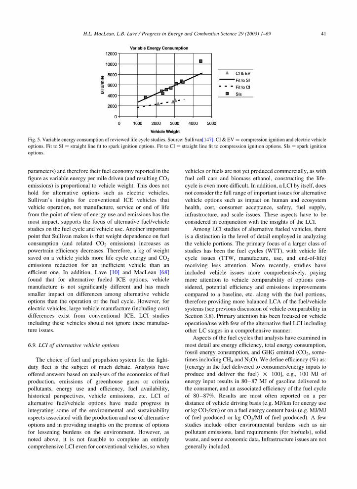
parameters) and therefore their fuel economy reported in the

figure as variable energy per mile driven (and resulting CO2

emissions) is proportional to vehicle weight. This does not

hold for alternative options such as electric vehicles.

Sullivan’s insights for conventional ICE vehicles that

vehicle operation, not manufacture, service or end of life

from the point of view of energy use and emissions has the

most impact, supports the focus of alternative fuel/vehicle

studies on the fuel cycle and vehicle use. Another important

point that Sullivan makes is that weight dependence on fuel

consumption (and related CO2 emissions) increases as

powertrain efficiency decreases. Therefore, a kg of weight

saved on a vehicle yields more life cycle energy and CO2

emissions reduction for an inefficient vehicle than an

efficient one. In addition, Lave [10] and MacLean [68]

found that for alternative fueled ICE options, vehicle

manufacture is not significantly different and has much

smaller impact on differences among alternative vehicle

options than the operation or the fuel cycle. However, for

electric vehicles, large vehicle manufacture (including cost)

differences exist from conventional ICE. LCI studies

including these vehicles should not ignore these manufac-

ture issues.

6.9. LCI of alternative vehicle options

The choice of fuel and propulsion system for the light-

duty fleet is the subject of much debate. Analysts have

offered answers based on analyses of the economics of fuel

production, emissions of greenhouse gases or criteria

pollutants, energy use and efficiency, fuel availability,

historical perspectives, vehicle emissions, etc. LCI of

alternative fuel/vehicle options have made progress in

integrating some of the environmental and sustainability

aspects associated with the production and use of alternative

options and in providing insights on the promise of options

for lessening burdens on the environment. However, as

noted above, it is not feasible to complete an entirely

comprehensive LCI even for conventional vehicles, so when

vehicles or fuels are not yet produced commercially, as with

fuel cell cars and biomass ethanol, constructing the life-

cycle is even more difficult. In addition, a LCI by itself, does

not consider the full range of important issues for alternative

vehicle options such as impact on human and ecosystem

health, cost, consumer acceptance, safety, fuel supply,

infrastructure, and scale issues. These aspects have to be

considered in conjunction with the insights of the LCI.

Among LCI studies of alternative fueled vehicles, there

is a distinction in the level of detail employed in analyzing

the vehicle portions. The primary focus of a larger class of

studies has been the fuel cycles (WTT), with vehicle life

cycle issues (TTW, manufacture, use, and end-of-life)

receiving less attention. More recently, studies have

included vehicle issues more comprehensively, paying

more attention to vehicle comparability of options con-

sidered, potential efficiency and emissions improvements

compared to a baseline, etc. along with the fuel portions,

therefore providing more balanced LCA of the fuel/vehicle

systems (see previous discussion of vehicle comparability in

Section 3.8). Primary attention has been focused on vehicle

operation/use with few of the alternative fuel LCI including

other LC stages in a comprehensive manner.

Aspects of the fuel cycles that analysts have examined in

most detail are energy efficiency, total energy consumption,

fossil energy consumption, and GHG emitted (CO2, some-

times including CH4 and N2O). We define efficiency (%) as:

[(energy in the fuel delivered to consumers/energy inputs to

produce and deliver the fuel) £ 100], e.g., 100 MJ of

energy input results in 80–87 MJ of gasoline delivered to

the consumer, and an associated efficiency of the fuel cycle

of 80–87%. Results are most often reported on a per

distance of vehicle driving basis (e.g. MJ/km for energy use

or kg CO2/km) or on a fuel energy content basis (e.g. MJ/MJ

of fuel produced or kg CO2/MJ of fuel produced). A few

studies include other environmental burdens such as air

pollutant emissions, land requirements (for biofuels), solid

waste, and some economic data. Infrastructure issues are not

generally included.

Fig. 5. Variable energy consumption of reviewed life cycle studies. Source: Sullivan[147]. CI & EV ¼ compression ignition and electric vehicle

options. Fit to SI ¼ straight line fit to spark ignition options. Fit to CI ¼ straight line fit to compression ignition options. SIs ¼ spark ignition

options.


The aspects of the vehicles receiving most attention are

vehicle fuel economy (efficiency), GHG emissions, oper-

ational energy use, and vehicle exhaust emissions of

regulated pollutants. A number of recent studies assume

that all vehicle options are able to meet near term US or

European emissions standards (since this is required if they

are to be sold), rather than estimating emissions from the

various vehicle options.

Some of the earliest LCI models for alternative

fuel/propulsion system options were developed by Mark

Delucchi at University of California at Davis during the

period 1987–1993. Delucchi has continued to update his

work [65,148]. Michael Wang of Argonne National

Laboratory has produced another LCI model [66]. Both

Delucchi and Wang’s models are spreadsheet—based life

cycle models that consider a large number of fossil and

biofuel/vehicle combinations for LDV [65,66,71,149, 175].

Delucchi’s spreadsheet model predicts emissions of GHG

and criteria pollutants from a large number of alternative

fuel/vehicle options. The model is comprehensive in scope

(including fuel cycles, vehicle operation, manufacture,

service, etc.) and requires significant input of details such

as energy usage for fuel production, emissions factors, etc.

Default values are also included. The updating of the work

has consisted primarily of improving fuel cycle energy and

fuel cycle and vehicle emissions estimates and adding new

fuel and vehicle options. Delucchi [150] is the most recent

work reporting air pollutant and GHG emissions results of

the model for highway vehicles, forklift trucks and house-

hold heating in the US. Delucchi’s model has been adapted

for Canada as a project for Natural Resources Canada [151]

followed by additional adaptation by Levelton Consulting of

Vancouver, B.C. [152].

Michael Wang’s work dates back to 1995 and has been

updated with additional information, parametric assump-

tions, fuel, and vehicle options. GREET (Greenhouse gases,

Regulated Emissions and Energy Use in Transportation), as

Wang’s model is called, estimates energy use (total, fossil,

petroleum) and emissions (GHG and criteria pollutants)

resulting from the LC of alternative transportation fuels and

vehicles but like Delucchi, primarily focuses on the fuel

cycle (WTT) aspects. These models have been utilized or

are the basis (with some modifications) for many of the other

LCI studies [68,70].

Wang [66] provides a good summary and qualitative

comparison of a number of the prominent alternative fuel

studies up to 1999 that focused on the fuel cycles. These

include Refs. [65,71,100,149,153–162]. The studies focus

on fuels and electricity for vehicle use and vary in their level

of detail, number of options considered, geographical

location, study assumptions and results. Wang reported

that the Delucchi and Acurex studies are the most

comprehensive in terms of fuels and technologies. Other

studies consider smaller numbers of fuel and vehicle options

but may be more comprehensive with respect to particular

options than Delucchi and Acurex.

6.10. Evaluation of LCI alternative fuel/propulsion system

option LCI studies

We evaluate and compare a number of recent alternative

fuel/vehicle LCI studies. Are methods and results similar?

What overall insights regarding vehicles and fuels can be

gained? What insights do we get with regard to LCI? We

compare the studies qualitatively, and where possible,

quantitatively. Due to the complexity of the studies,

differences in fuels and vehicles considered, technology

assumptions, lack of comparability of vehicles, differences

in metrics reported, activities considered, and incomplete

reporting of study methods, models and data, meaningful

comparisons are difficult. The studies cannot be classified

usefully by comparing a small number of metrics; results are

dependent on a large number of assumptions regarding the

fuel/vehicle systems. However, on a more positive note,

important insights are gained from a comparison.

We select a broad set of recent LDV LCA studies that

include reasonably comprehensive sets of conventional and

alternative vehicle options and that utilize a reasonably

balanced approach to treating the fuel/vehicle system. We

consider the studies in chronological order as follows:

Kreucher [75], IEA [163], Levelton [164], Lave [10] and

MacLean [68], MIT [69], Hackney [78], GM/Argonne [70,

178], and Delucchi [150]. These studies focus on fuels and

vehicles that have the potential to be commercialized in

large volumes within the near term (10–20 years). With a

few exceptions (e.g. LPG, BPV), fuels and propulsion

systems that appear to be commercially viable only in niche

markets were not considered. With the exception of Lave

[10], who employed the EIO-LCA model for some aspects

of the LCI, all other studies utilized the conventional LCA

process model method. In addition to the LCI portion of the

studies, Levelton [165], Lave [10] and MIT [69] included

some consideration of vehicle affordability. Results for

gasoline and diesel from Ref. [165] (Joshi, ADL and

Hoehlein) are also presented in Figs. 6 and 7 for comparison

purposes. We also include in the comparison, recent studies

that examined smaller sets of alternative vehicle options.

These studies include Refs. [77,79,104,166]. Hydrogen

FCV offer the possibility of being highly efficient ‘zero

emission vehicles’. Thus, analysts are eager to investigate

this potential through LCI. The last three studies focus on

options for FCV, comparing these to conventional vehicles.

One of the primary difficulties is that that no FCV (not even

those that use liquid HC fuels, reforming them to hydrogen)

are being produced on a commercial scale (barely at a

prototypical scale) and significant breakthroughs in both

fuel and vehicle technology are required before they will be

produced. There is very limited data publicly available for

fuel cell technologies. LCA of products not yet fully

developed for the market are the most difficult, and results of

these studies must be analyzed carefully.

Table 4 shows the fuel/vehicle options and fuel feed-

stocks considered in the various studies.


6.11. Evaluated LCI studies

The following are short summaries of each of the studies

to supplement the entries of Table 5.

Kreucher [75] is a North American focused study (but

resulted from a similar study of options for China by the

Chinese government and Ford Motor Company [179]). The

study is an LCI reporting energy efficiency and emissions of

GHG and criteria pollutants. Kreucher also included

economic estimates for the vehicles, operation, and fuels.

Fuel cycle emission estimates were based on a spreadsheet

model by A.D. Little, supplemented with estimates from

publicly available information. Vehicle options were

modeled with Ford software and based on a Ford Escort

gasoline vehicle with 31.5 mpg.

IEA [163] reports the results of a study by the

International Energy Agency that compared the alternative

fuel systems with a world-wide focus for 1–5 and 15–25

years in the future. Primary emphasis was placed on the fuel

cycles, although vehicle operation was included. Energy

consumption, GHG and criteria pollutant emissions were

reported based on an evaluation of published study results

and assumptions about alternative vehicle efficiencies. The

baseline vehicle was a gasoline SI car. Results are reported

by setting the baseline vehicle equal to 100 and deviations

from this baseline for the metrics are presented based on this

scale. IEA notes that actual physical units are not directly

comparable, therefore, it is not possible to include the

quantitative results in our comparison.

Levelton [164] reports the results of a study commis-

sioned by the Transportation Table of the National Climate

Change Process for Canada. It investigated the role that

alternative and future petroleum fuels could play in reducing

GHG emissions from light and heavy-duty vehicles in

Canada and the US for the time frames 2000, 2010, and

2020. Included were estimates of GHG and criteria pollutant

emissions from fuel production, vehicle operation and

manufacture, as well as fuel and vehicle costs. Cost-

effectiveness measures for reduction of GHG emissions with

the various options were based on the effects of differential

prices in fuels and vehicles (excluding taxes). The baseline

vehicle was a SI passenger car fueled with 300-ppm sulfur

Fig. 6. Gasoline fuel cycle (well-to-tank) efficiencies reported in life cycle studies. GM ¼ baseline gasoline [70], GM future gas ¼ future

gasoline [70], MIT low S ¼ low sulfur gasoline [69], Brekken ¼ Brekken [77], Ogden ¼ Ogden [104], Kreucher ¼ Kreucher [75], MacLean

con ¼ conventional gasoline [68]. MacLean CaRFG2 ¼ California Phase 2 reformulated gasoline [68], ADL ¼ study by ADL reported in Joshi

[165], Levelton 2000 ¼ Levelton baseline gasoline [164], Levelton 2010 ¼ Levelton year 2010 gasoline, Delucchi RFG ¼ Delucchi

reformulated gasoline [150].

Fig. 7. Diesel fuel cycle (well-to-tank) efficiencies reported in life cycle studies. GM current ¼ current diesel [70], GM future ¼ future diesel

[70], MIT low S ¼ low sulfur diesel [69], Kreucher ¼ Kreucher [1998], MacLean EC diesel ¼ ARCO emission control diesel [68], Hoehlein

reported in Joshi [165], IEA 99 ¼ IEA [163], Wang ¼ Wang [66], Joshi ¼ Joshi [165], ADL ¼ study by ADL reported in Joshi [165],

Delucchi ¼ Delucchi [150].


gasoline. Data sources included published studies and a

Canadian version of the Delucchi model.

Lave [10] and MacLean [68] examined the LC economic

and environmental implications of options expected to be

available over the next two decades for powering a large

proportion of the US light-duty fleet. Lave utilized the EIO-

LCA model for vehicle options, supplemented with fuel cycle

data from Ref. [66] with adjustments by the authors. Energy

use (total and fossil), GHG, and criteria pollutant emissions

were reported for the LC. The baseline vehicle was a 1998

Ford Taurus sedan fueled with conventional federal gasoline.

MIT [69] assessed likely technologies for US passenger

cars for the year 2020 that could benefit from most

economies of scale. The study included energy, GHG, and

economic factors over the life cycles of the fuel/vehicle

options. Impacts of the technologies on the ‘main stake-

holder groups’—fuel manufacturers and distributors,

vehicle manufacturers and distributors, customers, and

governments, were assessed. An important aspect of this

study, differentiating it from the others, is the assumption of

an ‘evolved baseline’ gasoline ICE vehicle for the year

2020. This baseline was modeled from a 1996 vehicle

similar to a Toyota Camry but has substantial evolutionary

improvements in fuel economy (43.2 mpg) and GHG

emissions (about 1/3) and vehicle weight reduction (vehicle

weight is 1236 kg) compared to the baseline, assumed at 5%

additional cost. The efficiency improvements result from

assumed advances in the efficiency of the engine and

transmission, and in the areas of drag and rolling resistance,

as well as the use of lightweight materials. The vehicle was

fueled with low sulfur gasoline. The vehicle modeling was

based on updated versions of Matlab Simulink programs

originally developed at ETH, Zurich [167] and the fuel

cycles based on published data. Fuel and vehicle economic

issues were included in the study.

Hackney [78] developed and presented a LC spreadsheet

model for comparing criteria pollutant, GHG emissions,

energy use and cost of alternative fuel/vehicle options. The

data sources for the spreadsheet included ADL [168], and

extensions by Hackney [186] based on Delucchi [187] and

Wang [159] along with others noted. The focus of the study

was model development but reference values from pub-

lished studies were given so the publication does include

results and insights for the various options. The time frame

was not specifically defined, but was characterized as ‘near

term’. The baseline vehicle was a gasoline SI subcompact

passenger car with a fuel economy of 30 mpg. Results of the

study are presented graphically and therefore cannot be

translated into numerical values for quantitative comparison

with the other studies.

GM/Argonne [70] combined the fuel cycle model of

Argonne National Laboratory with modeling of vehicle

options using proprietary GM software, therefore achieving

a more balanced treatment of fuel and vehicle than most

studies. The overall assessment of the vehicle options was

based on their potential for improving fuel economy and

lower GHG emissions while maintaining the vehicle

performance demanded by North American consumers.

The study time frame was 2005–2010 and the baseline

vehicle a 2000 Chevrolet Silverado full size pickup truck

using low sulfur gasoline, having a fuel economy of

20.2 mpg.

Table 4

Summary of fuel/vehicle options considered in studies

Fuel feedstock Gasoline Diesel LPG CNG Methanol Ethanol Electricity GH2/LH2

Petroleum 1SF, 2S, 3SH,

4SDFH, 5SHF, 7SFH,

8SF, 9S, 10SF, 11F,

12F, 13SF, 14SHF

1CF, 2C,

3CH, 4C,

5CH, 7CH,

8C

1S, 2S,

3S, 8S

8B

Coal 8SF 8B

NG 5CH, 8C,

13F

8S 1S, 2S, 3S,

4SD, 5HS,

7S, 8S, 9S

1SF, 2SCF,

3SF, 5F, 7F,

8SF, 10F,

11F, 12F, 13F

8B 3F, 5F, 7F,

8SF, 9F, 10F,

11F, 12F,

13F, 14F

Food crops 2C, 8C 1S, 2SC, 3S, 8S

Biomass 2SCF, 8SF 1S, 2SC, 3S, 4S,

7SFH, 8SF

8B

US mix,

other mix

for elect.

1B, 3B,

5B, 14B

2SF, 3F, 7F,

10F, 12F,

13F

Renewable

for elect.

8B 3F, 8SF

Number indicates study number. 1: Ref. [150], 2: Ref. [70], 3: Ref. [78], 4: Ref. [163], 5: Ref. [75], 6: Ref. [10], 7: Ref. [152], 8: Ref. [69], 9:

FEA (1999), 10: Ref. [173], 11: Ref. [166], 12: Ref. [104], 13: Ref. [79], 14: Ref. [77]. S: spark ignition port injection engine, D: spark ignition

direct injection engine, C: compression ignition direct injection engine, H: hybrid electric (internal combustion engine and electric motor), F:

fuel cell, B: battery-powered.


Table 5

Fuel/vehicle life cycle study summary table

Referencea Location,time frameb

Baselinevehiclec

Vehiclemodelingd

Fuel cyclemodelinge

Life cyclestages includedf

Energyuse/efficiencyg

GHGh Airpollutantsi

Econ.j Uncert.sens.k

Compareresultsl

[75] US near term Escort gasoline 31.5 mpg Ford proprietary model A.D. little F, O, M Incl. Incl., mainlyCO2

Incl. Incl. Not incl. Not incl.

[163] IEA countries2000–05, 2015–25

Current gasolineICE car

Published data Published data F, O Incl. Incl. Incl. Notincl.

Not incl. Not incl.

[164] Canada, US 2000,10, 20

Current gasolineICE car, 300 ppm S

Published studies incl.Delucchi, Brekken

Canadian model basedon Delucchi withown modif.

F, O, M Not incl. Incl. Incl. Incl. Not incl. Not incl.

[10] US 2015–20 1998 Ford Taurus gasoline Own modeling [5] Argonne GREET withauthor modif.

F, O M, S, F, E(ICE options only)

Incl. Incl. Incl. Incl. Not incl. Not incl.

[69] US 2020 2020 gasoline car basedon 1996 Camry with evol.Improv. 43.2 mpg

Updated verson of MatlabSimulink,originally createdby ETHZurich

Published studies F, O, M, S, E Incl. Incl. Incl. Incl. Limited Not incl.

[78] US, near term Current gasolineICE car 30 mpg

Own model Based on Ref. [168],Delucchi 89, Ref. [159]others

F, O Incl. Incl. Incl. Incl. Limited Not incl.

[70] US, 2005–10 Current Silverado lowS gasolinepickup, 20.2 mpg

GM proprietary model Argonne GREET model F, O Incl. Incl. Not incl.(but incl.in Argonnemodel)

Notincl.

Incl. Not incl.

[150] US, 2000, 2020 Current gasoline ICE car,25 mpg

Own model Delucchi model F, O, M No, butobtainedfromDelucchi

Incl. Incl. Notincl.

Not incl. Limited

[77] US near term 1997 Taurus, gasoline ICE23.2 mpg

Own model based onpub. studies

Own model based onpub. studies

F, O Incl. Not incl. Not incl. Notincl.

Limited Limited

[104] US near term Car Own model Published studies andown model

F, M Incl. Not incl. Incl. Incl. Not incl. Not incl.

[166] Canada, US 2010 ICE car, 30 ppm gasoline Directed technologies Inc.model [169]

Canadian model basedon Delucchi

F, O, M Not incl. Incl. Incl. Not incl. Not incl. With Refs.[79,152]

[79] Canada, US Current Mercedes BenzA-class, RFG, 7.3 l/100 km

Own model, PembinaLCVA

Published studies F, O Not incl. Incl. Incl. Not incl. Not incl. Not incl.

Table includes life cycle studies of alternative fuel/propulsion system options. Fuels and vehicle types included in the studies are reported in Table 4.a Study designation/reference.b Geographical area(s) and time frame(s) considered in study.c Baseline vehicle and fuel with which fuel/vehicle options are compared, fuel economy also reported where available. ICE: internal combustion engine, RFG: reformulated gasoline, S: sulfur.d Modeling/data source for vehicles.e Modeling/data source for fuel cycles.f Life cycle stages included; F: fuel cycle, O: vehicle operation/driving, M: vehicle manufacture, S: service, F: fixed costs, E: end-of-life.g Whether energy use is reported in the study.h Whether greenhouse gas emissions are reported in the study.i Whether criteria and/or toxic pollutant emissions are reported in the study.j Whether economic data are reported in the study.k Whether the study includes any uncertainty or sensitivity analyses.l Whether the study includes any comparisons of results with other studies.

H.L

.M

acL

ean

,L

.B.

La

ve/

Pro

gress

inE

nerg

ya

nd

Co

mb

ustio

nS

cience

29

(20

03

)1

–6

94

5

Delucchi [150] presented LCI results for the US for years

2000 and 2020 (with a focus on fuel cycle and vehicle

operation) of GHG emissions and urban pollutants from a

range of alternative fuel and feedstock combinations for LDV.

The baseline vehicle was a current gasoline SI ICE passenger

car with a fuel economy of 25 mpg. Delucchi utilized his own

model for the work. Delucchi included a broader set of GHG

than other studies, including not only CO2, CH4 and N2O but

also chlorofluorocarbons and hydrofluorocarbons. Delucchi

does not include energy use in this work but provided these

results from his model to the authors.

Brekken [77] compared the efficiency (GHG emissions

are not included) of the fuel cycles and vehicle operation of a

small set of near term light-duty options for the US. Fuel

cycle efficiencies were taken from published literature and

Brekken models the vehicles based on required power to

weight ratio, vehicle range, and base weight. The baseline

vehicle was a 1997 Ford Taurus SI with 23.2 mpg fuel

economy running on conventional gasoline.

Ogden [104] focused on FCV and fuel infrastructure

design. Fuel cell, PNGV type, midsize automobiles with

reduced weight, rolling resistance and aerodynamic drag

fueled with hydrogen, methanol, and gasoline were modeled

and analyzed. In most cases the vehicles were fuel cell HEV.

Ogden developed a computer simulation model for the

vehicles (including onboard fuel processors) to calculate

vehicle performance, fuel economy and cost for the various

options. Unlike the majority of other studies, Odgen developed

capital cost estimates for refueling infrastructure development

for the fuel options. Although Odgen’s study is not a LCI, we

include it since it has a comparable portion and the study offers

insights into the attractiveness of FCV options.

Methanex [166] assessed emissions of GHG from FCVs

for both Canada and the US, comparing them with those from

a gasoline ICE vehicle. The study modeled ‘best technology

expected to be commercially available’ in the year 2010 for

both the fuel cell and conventional vehicle options. The SI

ICE ran on 30 ppm sulfur gasoline. The vehicles are modeled

based on Directed Technologies Inc. model [169] and fuel

cycles are based on the Canadian version of the Delucchi

model with refinement.

Pembina [79], a study by the Pembina Institute for

Appropriate Development of Alberta, Canada, compared five

‘near term fuel supply opportunities’ for FCV systems with a

Mercedes Benz A-Class ICE (7.3 l/100 km) using California

Phase II RFG. Options included onboard RFG and methanol

fuel processing, centralized and decentralized NG reforming,

and decentralized electrolysis. Only GHG emissions were

considered in the study, and unlike the other studies, the

functional unit for this study was 1000 km traveled by the

vehicle. The study used the LCI approach but does not

include vehicle manufacture. Pembina used their own model,

Pembina LCVA, to model the vehicles and ‘best available

public domain data sets’ for the fuels.

Six of the studies included some cost estimates associated

with vehicles and fuels (Hackney, Kreucher, Lave, Levelton,

MIT, and Ogden) and four of the studies included limited

uncertainty or sensitivity analysis (GM, Hackney, MIT, and

Brekken).

6.12. Comparison of LCI studies

All of the above studies are most detailed in the

information they provide on the WTW energy use/efficiency

and GHG emissions. A number of the studies include vehicle

manufacture and a small number include other aspects of the

LC (e.g. service, end-of-life). Although the vast majority of

energy use, GHG and criteria pollutant emissions result from

vehicle operation, and secondarily from the WTT portion of

the LC for ICE vehicles, this is not as clearly the case for

electric vehicles. In addition, environmental burdens other

than those cited above may be important for decision

makers, e.g. solid waste generation, fossil fuel and other

resource consumption. Therefore, although we focus our

comparison on fuel cycle (WTT) and vehicle operation

(TTW) aspects, we do not imply that the other LC

components should be given less attention. However, at

this time, little detail is available for the other LC stages for

vehicles other than ICE.

For our quantitative portion of the comparison, due to data

availability, we only consider the WTT and TTW com-

ponents of the LCIs. Figs. 6–18 and Table 6 (Section 6.12.1)

report the study results for the WTT portion for the various

fuels. Figs. 19–24 and Table 7 (Section 6.12.2) report the

study results for the well-to-wheel—WTW (the sum of the

WTT and the TTW portions) portion for the fuel/propulsion

systems considered. We first consider the WTT portion and

examine the results for the various studies.

6.12.1. Fuel cycles (well-to-tank—WTT)

Although analyzing the results of the various fuel cycles

is more straightforward than analyzing the results of vehicle

operation (due to the lack of comparability of vehicles and

their complexity), comparability aspects complicate the fuels

analyses as well. Insights gained from isolating any

component of the LC must be evaluated only when taking

into consideration the entire LC, systems approach. No

single metric can adequately describe the WTT aspects of

any fuel. For example, assumptions regarding production

and level of sulfur in gasoline or diesel, feedstock source

assumptions and percentage of fossil fuel assumed used to

produce ethanol, hydrogen fuel production pathways,

electricity generation mixes all significantly impact fuel

cycle results. All of these issues make it necessary to

carefully evaluate the WTT and a variety of metrics

important to the decision maker before coming to con-

clusions about the attractiveness of a fuel. The aspect that

makes comparing the fuels (WTT portion) more straightfor-

ward than the TTW portion, is that we know that 1 MJ of

hydrogen produced by electrolysis is equivalent to 1 MJ of

hydrogen produced from natural gas as far as propelling the

vehicle a certain distance.


The majority of the studies only report quantitatively,

efficiency (or energy use) and GHG emissions. This limits

the scope of our quantitative comparisons to these two

metrics. Where efficiency as a proportion is not reported, we

calculate it from the number of MJ of fuel delivered to

consumer divided by the number of MJ of process energy

input. GHG are usually reported in the studies in grams CO2

equivalent/MJ or MMBtu of fuel with CO2, CH4, and N2O

considered and weighted by their GWP. However, there are

a few exceptions where only CO2 is considered, where

additional GHG are included, or where the GWP are slightly

different than the usual 100-year International Panel on

Climate Change (IPCC) values of 21 for CH4 and 310 for

N2O [150]. We have adjusted results where possible to

provide a consistent comparison. Table 6 provides an

overall summary of the ranges of the efficiencies and GHG

emissions for the WTT portions for the fuels reported in the

LC studies. The values in the table are taken from Figs.

6–18 discussed in this section.

Overall, a portion of the similarity in results for many of

the fuels occurs because several of the studies take results

from the models of Wang and Delucchi (e.g. Lave [10]/

MacLean [68] and GM/Argonne [70] use Wang with some

modifications, Levelton [164] uses Delucchi with modifi-

cations to make the analysis applicable to Canada).

For conventional petroleum-based fuels, fuel cycle

pathways are reasonably straightforward, while fuels like

hydrogen and ethanol have many alternative fuel cycle

options (different feedstocks, processes, distributions,

etc.), resulting in much less variation in results among

options for the former fuels. We must keep in mind when

interpreting the following fuel cycle results that a MJ of

gasoline is not equivalent to a MJ of hydrogen for use in a

vehicle due to the different efficiencies of the vehicle

powerplants.

All of the studies use gasoline from petroleum feedstock

as the baseline fuel. However, the fuel characteristics,

whether it is low sulfur, reformulated, has an oxygenate, etc.

differ among the studies examined. While the majority of

studies are for the US, several are for other geographical

areas which contributes to differences in the results. Even

with all of these differentiating factors, the results for the

gasoline fuel cycles efficiencies all range between 80 and

87% (mean ¼ 83), with one exception at 94% [104] (Fig. 6).

Fig. 8. CNG fuel cycle (well-to-tank) efficiencies reported in life cycle studies. GM NANG ¼ North American natural gas [70], MIT ¼ MIT

[69], Kreucher ¼ Kreucher [75], MacLean ¼ MacLean [68], Brekken ¼ Brekken [77], GM NNA NG ¼ non North American natural gas [70],

IEA ¼ IEA [163], Delucchi ¼ Delucchi [150].

Fig. 9. Methanol fuel cycle (well-to-tank) efficiencies reported in life cycle studies. GM NA, NG ¼ source of methanol is North American

natural gas [70], GN NNA NG ¼ source is non North American natural gas [70], MIT NG ¼ source is natural gas [69], Ogden ¼ source not

specified [104], Kreucher NG ¼ source is natural gas [75], IEA NG ¼ source is natural gas [163], Delucchi NG ¼ source is natural gas [150],

IEA cellulosic ¼ source is cellulosic feedstocks [163].


Whether the efficiency is 80 or 87 does not impact the

overall attractiveness of gasoline significantly. There is not

sufficient detail in Ogden to provide a definitive answer

regarding the source of the difference in Ogden’s estimate.

However, Ogden assumes that the conversion of petroleum

in the refinery to gasoline is 95% and that the truck delivery

energy is 1% of total energy required as being inputs into the

statement that ‘for 100 units of primary energy input, 94

units of gasoline energy are delivered to the vehicle’ [104,

p. 152]. The higher value results in part from assuming a

higher refining efficiency than the other studies. For

example, MIT [69] assumes a value of 86.6% for refining

efficiency. However, this value appears to be on the low side

due to the MIT assumption of additional energy use for

producing very low sulfur gasoline.

Results for GHG emissions for gasoline (Fig. 13) range

from 15 g CO2/MJ of fuel for Kreucher (only considering

CO2) to over 25 g CO2 equiv/MJ for Methanex’s no sulfur

gasoline. As expected, within a particular study an increase

in GHG emissions is associated with a decrease in sulfur

content of the fuel due to the additional energy required for

removing sulfur. Sources of differences result from GHG

emissions considered (whether just CO2, or whether CH4 or

N2O or others are considered) and geographical location.

(Canadian emissions are generally slightly higher than those

for the US.)

The efficiencies for the diesel fuel cycles shown in Fig. 7

range from 83 to 90 (mean ¼ 88). The efficiency of diesel

production is slightly higher than that of gasoline, and this is

shown in the studies examined here. The variation in the

Fig. 10. Hydrogen fuel cycle (well-to-tank) efficiencies reported in life cycle studies. GM Central GH2 NA NG ¼ GM centralized gaseous

hydrogen from North American natural gas [70]; GM Central GH2 NNA NG ¼ centralized gaseous hydrogen from non North American natural

gas; GM Station GH2 NA NG ¼ station gaseous hydrogen from North American natural gas; GM Station GH2 NNA NG ¼ station gaseous

hydrogen from non North American natural gas; GM Station GH2 US Mix ¼ station gaseous hydrogen from US electricity generation mix; GM

Station GH2 NA NG CC ¼ station gaseous hydrogen from North American natural gas combined cycle; GM Central LH2 NA

NG ¼ centralized liquid hydrogen from North American natural gas; GM Central LH2 NNA NG ¼ centralized liquid hydrogen from non North

American natural gas; GM Stn LH2 NA NG ¼ station liquid hydrogen from North American natural gas; GM Stn LH2 NNA NG ¼ station

liquid hydrogen from non North American natural gas; GM Stn LH2 US Mix ¼ station liquid hydrogen from US electricity generation mix; GM

STN LH2 NA NG CC ¼ station liquid hydrogen from North American natural gas combined cycle; MIT CompH syn fr NG dec refuel ¼ MIT

compressed hydrogen synthesis from natural gas decentralized reforming [69]; Brekken ¼ Brekken [77]; Ogden H, NG steam ref. ¼ gaseous

hydrogen from natural gas steam reforming [104]; IEA H, electrolysis ¼ gaseous hydrogen from electrolysis [163]; Delucchi GH2

NG ¼ gaseous hydrogen from natural gas [150].

Fig. 11. Electricity generation (well-to-tank) efficiencies reported in life cycle studies. GM US mix ¼ source is average US electicity generation

mix [70], GM NA NG CC ¼ North American natural gas combined cycle plants, MIT national grid ¼ average US electricity generation mix

[69], Kreucher US ¼ average US electricity generation mix [75], Kreucher world ¼ average world electricity generation mix, Kreucher W.

Europe ¼ average Western Europe electricity generation mix, Kreucher CA ¼ California generation mix.


results is expected to result from differences in geographical

conditions, specific fuel production pathways, fuel compo-

sition, etc. Differences in sulfur content are expected to be a

primary differentiating factor, with the increase in process

energy required to lower the fuel sulfur level. Diesel fuel

WTT GHG emissions are shown in Fig. 14 and range from a

low of 7 g CO2/MJ of fuel for Kreucher to 18 g CO2/MJ for

MacLean [68] and GM future diesel. Both these studies

assume very low sulfur fuel. Consuming many MJ of fuel

with higher CO2 emissions could have a significant impact.

Results for CNG are shown in Fig. 8. This is another fuel

with a known pathway, with efficiencies ranging only from

83 to 91%, except for two outliers, GMs result for non-North

American production at 77% and the IEA estimate of 96%.

IEA provides large ranges of values for each of the fuel cycle

stages (e.g. 30–90 MJ/GJ for fuel distribution). Although the

median estimate is 96%, values reported in other studies fit

within the ranges give. GHG emissions are reported in Fig. 15

and fall between 10 g CO2/MJ for Kreucher and 27 g CO2

equivalent for the GM non-North American option. Since

Fig. 12. Ethanol fuel cycle (well-to-tank) efficiencies (total energy) reported in life cycle studies. GM corn ¼ ethanol feedstock is corn [70]; GM

woody ¼ feedstock is woody biomass; GM herb ¼ feedstock is herbaceous biomass; Lave Corn ¼ feedstock is corn [10]; Lave Herb.

Credit ¼ feedstock is herbaceous biomass, includes electricity credit; Lave herb no credit ¼ feedstock is herbaceous biomass, does not include

electricity credit; Lave woody credit ¼ feedstock is woody biomass, includes electricity credit; Lave woody no credit ¼ feedstock is woody

biomass, does not include electricity credit; Kreucher corn ¼ feedstock is corn [75]; Kreucher cell.biomass ¼ feedstock is cellulosic biomass;

Levelton 2000,corn ¼ year 2000, feedstock is corn [164]; Levelton 2010,corn ¼ year 2010, feedstock is corn; Levelton 2000,SG ¼ year 2000,

feedstock is switchgrass; Levelton 2010,SG ¼ year 2010, feedstock is switchgrass; Levelton 2000,stover ¼ year 2000, feedstock is corn stover;

Levelton 2010,stover ¼ year 2010, feedstock is corn stover, IEA cellulosic ¼ feedstock is cellulosic biomass [163]; IEA sugar/starch ¼

feedstock is sugar/starch; Delucchi 2000,corn ¼ year 2000, feedstock is corn [150]; Delucchi 2000,cell ¼ year 2000, feedstock is cellulosic

biomass.

Fig. 13. Gasoline fuel cycle (well-to-tank) greenhouse gas emissions reported in life cycle studies. GM ¼ baseline gasoline [70], GM

future ¼ future gasoline [70], MIT low S ¼ low sulfur gasoline [69], Kreucher ¼ Kreucher [75], MacLean con ¼ conventional gasoline [68],

MacLean CaRFG2 ¼ California Phase 2 reformulated gasoline [68], Methanex 30S ¼ 30 ppm sulfur gasoline [166], Methanex noS ¼ no sulfur

gasoline, Levelton 300S ¼ 300 ppm sulfur gasoline [164], Levelton 30S ¼ 30 ppm sulfur gasoline, Levelton 1S ¼ 1 ppm sulfur gasoline,

Delucchi 2000RFG ¼ year 2000 reformulated gasoline [150], Delucchi 2020RFG ¼ year 2020 reformulated gasoline.


Kreucher has not included methane in the calculation and

combustion of CNG releases substantial amounts of

methane, this significantly impacts the results.

Fuel production efficiency estimates for F–T diesel were

included in two studies, GM and MIT. GMs estimate of 59%

is somewhat more optimistic than MITs 52%. However,

the much lower efficiency of these fuel cycles compared to

those of conventional diesel should be noted.

Methanol was included in five studies, with natural gas

as the feedstock. All results were in the range of 56–66%

efficiency as shown in Fig. 9. IEA [163] also reports a result

for cellulosic feedstock (58%).

The GM/Argonne study considers the largest range of

options for production of both gaseous (six options) and

liquid (six options) hydrogen. The options include those

from NG both in North America and outside North

America, from electrolysis, and central vs. station options.

The efficiencies for the hydrogen fuel cycles are shown in

Fig. 10. Overall, as expected, the efficiencies for the

gaseous options are higher than those of the liquid options.

The central and station North American NG options have

the highest efficiencies, 57 and 56%, respectively.

However, these efficiencies are much lower than those of

conventional petroleum-based fuels. The lowest efficiency

option is the liquid hydrogen from electrolysis, US mix at

23%. This low efficiency results from compounding the

low efficiency of electricity generation with the additional

energy requirements of producing the hydrogen from the

electricity as noted earlier. MIT analyzes gaseous hydro-

gen produced from NG decentralized refueling resulting in

an estimate of 56%. Brekken assumes gaseous hydrogen

through NG reforming in an industrial plant and is more

optimistic at 65%; Ogden also assumes NG steam

reforming with an estimate of 76%. Delucchi [150] reports

hydrogen from natural gas at 44% efficiency. IEA assumes

production by electrolysis with a 31% efficiency. GHG

emissions from the hydrogen options vary greatly (Fig. 16).

Hydrogen produced using electrolysis and the US mix

have the highest emissions (265–332 g CO2/MJ fuel

produced) while the Canadian studies [164,166] and

Delucchi options from NG have the lowest estimates at

about 85 g CO2/MJ fuel. Levelton [164] option of

producing hydrogen using 100% hydroelectricity has

lowest overall emissions as would be expected. As is

Fig. 14. Diesel fuel cycle (well-to-tank) greenhouse gas emissions reported in life cycle studies. GM ¼ conventional diesel [70], GM

future ¼ future low sulfur diesel, MIT low S ¼ low sulfur diesel [69], Kreucher ¼ Kreucher [75], MacLean EC ¼ ARCO emission control (low

sulfur) diesel [68], Levelton 500S ¼ 500 ppm sulfur diesel [164], Levelton 50S ¼ 50 ppm diesel, Delucchi 2000 ¼ year 2000 diesel [150],

Delucchi 2020 ¼ year 2020 diesel.

Fig. 15. CNG fuel cycle (well-to-tank) greenhouse gas emissions reported in life cycle studies. GM NANG ¼ North American natural gas [70],

MIT ¼ MIT [69], Kreucher ¼ Kreucher [75], MacLean ¼ North American natural gas [68]. GM NNANG ¼ non North American natural gas,

Levelton ¼ Levelton [164], Delucchi 2000 ¼ year 2000 natural gas [150], Delucchi 2020 ¼ year 2020 natural gas.


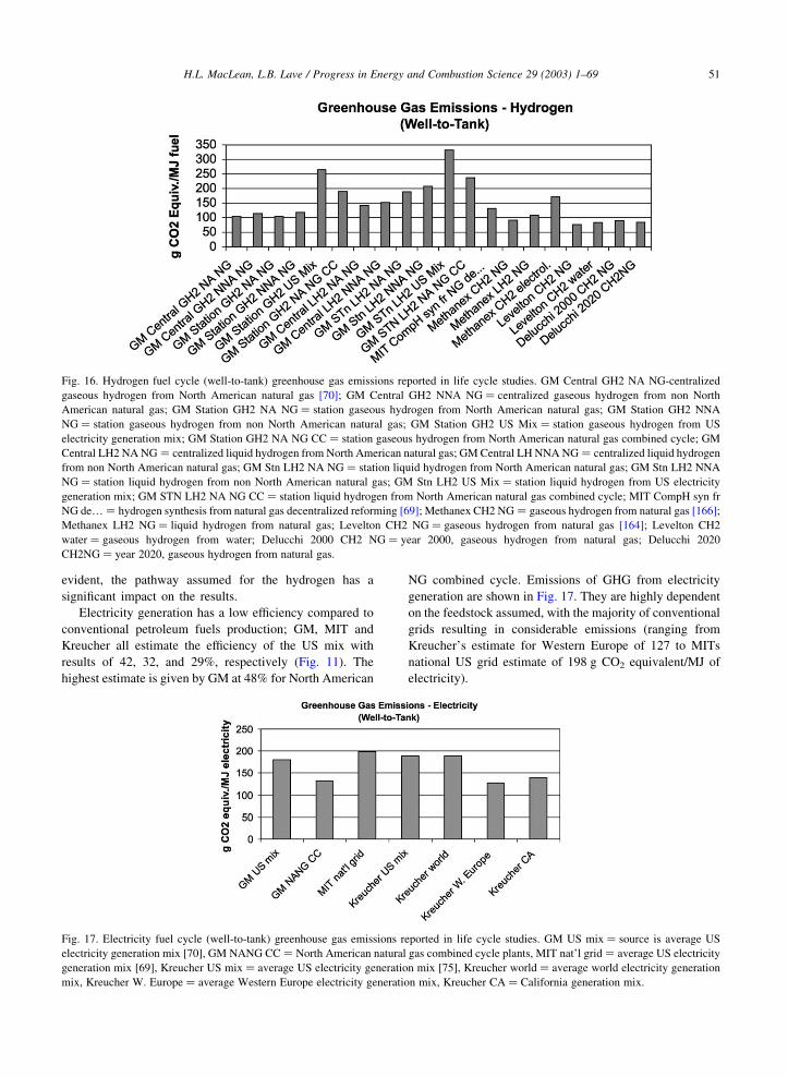
evident, the pathway assumed for the hydrogen has a

significant impact on the results.

Electricity generation has a low efficiency compared to

conventional petroleum fuels production; GM, MIT and

Kreucher all estimate the efficiency of the US mix with

results of 42, 32, and 29%, respectively (Fig. 11). The

highest estimate is given by GM at 48% for North American

NG combined cycle. Emissions of GHG from electricity

generation are shown in Fig. 17. They are highly dependent

on the feedstock assumed, with the majority of conventional

grids resulting in considerable emissions (ranging from

Kreucher’s estimate for Western Europe of 127 to MITs

national US grid estimate of 198 g CO2 equivalent/MJ of

electricity).

Fig. 16. Hydrogen fuel cycle (well-to-tank) greenhouse gas emissions reported in life cycle studies. GM Central GH2 NA NG-centralized

gaseous hydrogen from North American natural gas [70]; GM Central GH2 NNA NG ¼ centralized gaseous hydrogen from non North

American natural gas; GM Station GH2 NA NG ¼ station gaseous hydrogen from North American natural gas; GM Station GH2 NNA

NG ¼ station gaseous hydrogen from non North American natural gas; GM Station GH2 US Mix ¼ station gaseous hydrogen from US

electricity generation mix; GM Station GH2 NA NG CC ¼ station gaseous hydrogen from North American natural gas combined cycle; GM

Central LH2 NA NG ¼ centralized liquid hydrogen from North American natural gas; GM Central LH NNA NG ¼ centralized liquid hydrogen

from non North American natural gas; GM Stn LH2 NA NG ¼ station liquid hydrogen from North American natural gas; GM Stn LH2 NNA

NG ¼ station liquid hydrogen from non North American natural gas; GM Stn LH2 US Mix ¼ station liquid hydrogen from US electricity

generation mix; GM STN LH2 NA NG CC ¼ station liquid hydrogen from North American natural gas combined cycle; MIT CompH syn fr

NG de… ¼ hydrogen synthesis from natural gas decentralized reforming [69]; Methanex CH2 NG ¼ gaseous hydrogen from natural gas [166];

Methanex LH2 NG ¼ liquid hydrogen from natural gas; Levelton CH2 NG ¼ gaseous hydrogen from natural gas [164]; Levelton CH2

water ¼ gaseous hydrogen from water; Delucchi 2000 CH2 NG ¼ year 2000, gaseous hydrogen from natural gas; Delucchi 2020

CH2NG ¼ year 2020, gaseous hydrogen from natural gas.

Fig. 17. Electricity fuel cycle (well-to-tank) greenhouse gas emissions reported in life cycle studies. GM US mix ¼ source is average US

electricity generation mix [70], GM NANG CC ¼ North American natural gas combined cycle plants, MIT nat’l grid ¼ average US electricity

generation mix [69], Kreucher US mix ¼ average US electricity generation mix [75], Kreucher world ¼ average world electricity generation

mix, Kreucher W. Europe ¼ average Western Europe electricity generation mix, Kreucher CA ¼ California generation mix.


Ethanol results are highly dependent on the fuel pathway

and assumptions employed (e.g. whether electricity credits

given, use of lignin for heat in the process). Since only 2%

of commercial production of ethanol in the US has been

from biomass sources other than corn, assumptions and

results for the other pathways are more uncertain. Fig. 12

shows the WTT efficiency taking into account total energy.

We report, where possible, results for both total energy use

efficiency and also efficiency only including fossil fuel use

(Table 6). As expected, the attractiveness of lignocellulosic

ethanol improves significantly from an efficiency point of

view when just fossil fuel inputs are considered (due to the

potential of using lignin for process energy). In contrast,

corn results do not improve when only fossil fuels are

considered since corn does not have the lignin energy source

of the cellulosic feedstocks and the use of corn stover

which could provide some process energy is not assumed in

the studies. Ethanol has the potential to be produced

‘sustainably’ (defined here as no fossil fuel in the ethanol

fuel cycle, e.g. ethanol to fuel tractors), however, today’s

production does not follow this route. With total energy

considered, the corn cycles are more efficient than the

lignocellulosics (on the order of 65 vs. 40%) but the

situation reverses with fossil energy only considered (65 vs.

90%).

The potential with ‘sustainable’ production of no net

CO2 emissions resulting from the production and combus-

tion of ethanol is a primary driver behind the attractive-

ness of ethanol. Carbon is sequestered during biomass

growth and then released into the atmosphere with

Fig. 18. Ethanol fuel cycle (well-to-tank) greenhouse gas emissions reported in life cycle studies. GM corn ¼ ethanol feedstock is corn [70];

GM woody ¼ feedstock is woody biomass; GM herb ¼ feedstock is herbaceous biomass; Lave Corn ¼ feedstock is corn [10]; Lave

Herb.credit ¼ feedstock is herbaceous biomass, includes electricity credit; Lave herb no credit ¼ feedstock is herbaceous biomass, does not

include electricity credit; Lave woody credit ¼ feedstock is woody biomass, includes electricity credit; Lave woody no credit ¼ feedstock is

woody biomass, does not include electricity credit; Kreucher corn ¼ feedstock is corn [75]; Kreucher cell.biomass ¼ feedstock is cellulosic

biomass; Levelton 2010, agr res ¼ year 2010, feedstock is agricultural residues [164]; Levelton 2010,corn ¼ year 2010, feedstock is corn;

Delucchi 2000 corn ¼ year 2000, feedstock is corn [150]; Delucchi 2000 cell. ¼ year 2000, feedstock is cellulosic biomass; Delucchi 2020

corn ¼ year 2020, feedstock is corn; Delucchi 2020 cell. ¼ year 2020, feedstock is cellulosic biomass.

Table 6

Comparison of life cycle inventory studies: well-to-tank efficiencies and greenhouse gas emissions

Fuel/source (if applicable) Efficiency (%), range Greenhouse gas emissions (g CO2 equiv./MJ fuel), range

Gasoline 80–87 15–26

Diesel 83–90 12–18

FT-diesel 52–59 –

CNG 83–91 10–27

Methanol 57–66 22–41

Ethanol (corn): total energy 45–67 219 to þ90

Ethanol (corn): fossil energy 60–67 –

Ethanol (lignocell.): total energy 26–56 285 to þ14

Ethanol (lignocell): fossil 83–96 –

Hydrogen (various sources) 23–76 76–332

Electricity (various sources) 29–48 127–198

Table does not include outliers. Efficiency (%) is defined as: ((energy in the fuel delivered to consumers/energy inputs to produce and deliver

the fuel) £ 100), e.g. 100 MJ of energy input results in 80–87 MJ of gasoline delivered to the consumer.


combustion of the fuel in the vehicles. Results for GHG

emissions from the WTT portions of the studies (Fig. 18)

vary greatly from large negative amounts (resulting from

carbon sequestration during feedstock growth) in the GM

work, particularly for the woody biomass option to large

positive values (releases of GHG emissions from corn

ethanol production) for Delucchi. Since the corn ethanol

production utilizes large amounts of fossil fuels in its

production and in associated fertilizer production (off-

setting any carbon sequestration benefits), these results are

not unexpected.

Overall, the variation in GHG emissions from the various

ethanol studies results from several sources; the assumed

feedstock, the amount of fossil fuels used in the fuel

production (which generate CO2), consideration or exclu-

sion of N2O since there are significant amounts resulting

from fertilizer use essential to producing the fuel (more

fertilizer is required for corn than for lignocellulosic

feedstocks), assumptions about land use and carbon

sequestration, year of study (assumed technological

changes, particularly larger amounts of lignin used in

cellulosic ethanol production offsetting fossil fuel use), and

whether a credit is given for selling excess electricity to the

grid and therefore offsetting CO2 emissions from conven-

tional electricity generation.

Table 6 summarizes the ranges reported in the LC studies

for the WTT efficiencies and GHG emissions for each of the

fuels. The efficiencies are highest for the fossil fuels:

gasoline, diesel and CNG. In addition, due to their known

and set production pathways, the ranges reported for these

fuels are much smaller than those of the other fuels. All of

the fossil fuel production results in significant GHG

emissions. When only fossil energy is considered the

lignocellulosic ethanol WTT portion is highly efficient and

has the potential for low GHG emissions. Hydrogen results,

both for efficiency and GHG emissions, vary greatly from

moderate to low efficiency and moderate to very high GHG

emissions. Electricity generation using current generation

mixes for the US and Canada has a low efficiency and high

GHG emissions.

Fig. 19. Gasoline spark ignition port fuel injection vehicle well-to-wheel greenhouse gas emissions reported in life cycle studies. GM

pickup ¼ Silverado pickup truck [70], MIT 1996ref sedan ¼ 1996 model year reference sedan [69], MIT 2020 low S ¼ year 2020 low sulfur

gasoline fuelled sedan, MIT 2020advlow S ¼ year 2020 low sulfur gasoline advanced sedan, Methanex car ¼ automobile [166], Pembina

A-class ¼ A-class Mercedes [79], Lave Taurusconv ¼ conventional gasoline fuelled Ford Taurus sedan [10], Lave TaurusCaRFG2 ¼

California Phase 2 reformulated gasoline fuelled Ford Taurus sedan, Levelton300ppmS ¼ 300 ppm sulfur gasoline fuelled automobile [164],

Levelton 30ppmS ¼ 30 ppm sulfur gasoline fuelled automobile.

Fig. 20. Diesel compression ignition direct injection well-to-wheel greenhouse gas emissions reported in life cycle studies. GM ¼ Silverado

pickup [70], MIT lowS ¼ low sulfur fuelled sedan [69], Lave lowS ¼ low sulfur fuelled Taurus sedan [10], Levelton ¼ conventional diesel

fuelled vehicle [164], Levelton 50ppmS ¼ 50 ppm sulfur fuelled vehicle , MIT F-T ¼ Fischer–Tropsch diesel fuelled sedan [69].


6.12.2. Fuel cycles and vehicle operation (well-to-wheel,

WTW)

As mentioned above, comparing LC results for vehicle

options is difficult. The lack of comparability of vehicles

considered severely limits meaningful quantitative com-

parisons even for the basic metrics of energy use and GHG

emissions that are reported in the majority of studies. We

limit our WTW quantitative comparison to that of the GHG

emissions reported in the studies since many studies do not

report WTW efficiencies. These estimates include emissions

resulting from the WTT and TTW components of the LC.

When evaluating overall efficiency of fuel/vehicle

systems, it is necessary to consider both the efficiency of

fuel production and the efficiency of vehicle operation. With

conventional vehicles, the high efficiencies of the petroleum

fuel cycles are generally combined with the relatively low

efficiencies of ICE vehicles (on the order of 20% for

gasoline). For the FCVs, the opposite is true. A low

efficiency fuel cycle is combined with a higher efficiency

powerplant. However, the hydrogen production efficiencies

may be low enough to offset the high efficiencies of FCVs.

Table 7 (range values taken from Figs. 19–24) provides an

overall summary of the ranges for the WTW GHG emissions

for the fuel/propulsion systems examined in the studies.

Fig. 19 reports the WTW GHG emissions from gasoline

fueled SIPI vehicles. GHG emissions from the WTW of

current gasoline SIPI ICE sedans are on the order of

250–300 g CO2 equiv./km. The full range goes from just

under 150 to almost 350 g CO2 equiv./km. For gasoline, the

largest portion of the GHG emissions is CO2 that is emitted

in proportion to the amount of fuel used and is related to

vehicle weight. Therefore, results for the GM study showing

higher GHG emissions from the full size pickup truck and

for the MIT study showing much lower emissions from the

‘evolved’ (lighter with higher fuel economy sedan) vehicles

are as expected. Additionally, we remind the reader that the

results of the GM/Argonne analysis for all of the fuels, due

to their choice of a full size pickup truck, a less fuel efficient

vehicle than the ‘sedans’ evaluated in the other studies,

makes this study particularly difficult to compare with the

other studies. Small increases in GHG emissions for the

lower sulfur content gasolines are reported by Lave and

Levelton.

Trends for diesel vehicle emissions are similar to those

of the results for gasoline vehicles above (Fig. 20). Due to

the combined higher WTT efficiency of the diesel fuel cycle

and higher TTW efficiency of the CIDI vehicles (and the

only slightly higher carbon content of the diesel fuel), the

diesel options result in lower WTW GHG emissions (about

23% reduction for Levelton low sulfur options). Only one

result is given for F–T diesel [69], reporting slightly higher

GHG emissions than the low sulfur petroleum-based diesel.

Fig. 22. Diesel HEV well-to-wheel greenhouse gas emissions reported in life cycle studies. All vehicles have compression ignition direct

injection engines and electric motors.

Fig. 21. Gasoline HEV well-to-wheel greenhouse gas emissions reported in life cycle studies. All vehicles have spark ignition port fuel injection

engines and electric motors.


For HEV fueled with gasoline and diesel, GHG

reductions depend on the assumed increase in fuel economy

for these options compared to the baseline vehicle (Figs. 21

and 22). Diesel HEV have the potential of high efficiency

(low GHG emissions) since they combine the advantages of

the high powerplant efficiency of the diesel engine and the

improvement in efficiency possible with a HEV

configuration.

Of the FCV options, the LC studies include vehicles that

use hydrogen directly and those that reform methanol or

gasoline to hydrogen onboard the vehicle and then use the

hydrogen in the FC. Fig. 24 shows the WTW GHG

emissions for the hydrogen, methanol and gasoline FCVs.

The direct hydrogen options have the potential both for the

largest reductions and largest increases in GHG emissions.

This results from the variation in the WTT results and the

Fig. 24. Fuel cycle vehicles well-to-wheel greenhouse gas emissions reported in life cycle studies. GM HEV ¼ Silverado pickup fuel cell hybrid

electric [70], MIT HEV ¼ fuel cell hybrid electric sedan [69], Methanex ¼ fuel cell sedan [166], Pembina ¼ fuel cell Mercedes A-class [79],

Lave HEV ¼ fuel cell hybrid electric sedan [10], Levelton ¼ fuel cell sedan [164], Methanex CH2 ¼ automobile fuelled with gaseous

hydrogen from natural gas [166], Methanex LH2 ¼ automobile fuelled with liquid hydrogen from natural gas, Methanex CH2elect ¼

automobile fuelled with gaseous hydrogen from electrolysis, Pembina Ngref. ¼ Mercedes A-class equivalent fuelled with gaseous hydrogen

from natural gas reforming (centralized) [79], Pembina Ngref.dec ¼ Mercedes A-class equivalent fuelled with gaseous hydrogen from natural

gas reforming (decentralized), Pembina dec.el ¼ Mercedes A-class equivalent fuelled with gaseous hydrogen from electrolysis (decentralized),

Levelton H NG ¼ fuel cell automobile fuelled with gaseous hydrogen from natural gas [164], Levelton H elect ¼ automobile fuelled with

gaseous hydrogen from electrolysis, average electricity generation mix, Levelton H elect hydro ¼ automobile fuelled with gaseous hydrogen

from electrolysis, 100% hydro power.

Fig. 23. Ethanol spark ignition vehicle well-to-wheel greenhouse gas emissions reported in life cycle studies. GM E85 cell. ¼ E85 (85%

ethanol, 15% gasoline), ethanol from cellulosic feedstock [70]; Lave E100 SIDI cell ¼ E100 (100% ethanol) in spark ignition direct injection

engine, ethanol from herbaceous cellulosic feedstock (with electricity credit) [10]; Lave E100 SIDI cell ¼ as above except with no electricity

credit; Lave E100 SIDI cell ¼ as above except from woody feedstock with electricity credit; Lave E100 SIDI cell ¼ as above except without

electricity credit; Levelton E85 corn ¼ E85 from corn feedstock [164]; Levelton E85 cell. ¼ E85 from cellulosic feedstock.


vehicle efficiencies. The use of hydrogen directly,

eliminates the need for energy to power a fuel reformer,

therefore lowering GHG emissions. Some of the hydrogen

FC WTW options emit more GHG than conventional

vehicles. Due to the Levelton [164] assumption of

producing the hydrogen through electrolysis using hydro-

power, this WTW estimate is small. Pembina reports the

lowest hydrogen FC GHG emissions from NG (70–80 g

CO2 equiv./km). These estimates are considerably lower

than those of the other studies. There is not sufficient detail

presented in the studies to determine the sources of the

difference.

Fig. 24 shows that the results for the GHG emissions

from the WTW for the methanol FC vehicles are generally

lower than those of the gasoline FCV. The processing of the

methanol onboard the vehicle results in lower GHG

emissions per kilometer than for gasoline reforming due to

the lower carbon content of methanol and the higher

methanol reformer efficiency. The lower gasoline WTW

GHG emissions estimate of Lave [10] is due in part to the

assumption of a smaller vehicle (e.g. Toyota Corolla) than

the other studies.

The two options that have potential for the largest GHG

emissions reductions are the ethanol (Fig. 23) and hydrogen

fueled vehicles (Fig. 24) if the fuels are produced with little

or no fossil fuel inputs. Results depend on the issues

discussed in Section 6.12.1) regarding WTT assumptions, as

well as ethanol blend assumptions (% gasoline) and engine

efficiency. For the ethanol vehicle, Lave [10] assumes a SIDI

engine and associated thermal efficiency improvements over

a conventional port fuel injection. However, we are not

aware of any experience with ethanol in DI engines.

Table 7 summarizes the ranges for the WTW GHG

emissions reported in the LC studies. Since the GM/

Argonne [70] and MIT [69] studies have vehicles that have

considerably different performance than the automobiles

examined in the remainder of the studies (for GM, the

Silverado pickup truck and for MIT, an advanced sedan for

the baseline), we report these results separately from the

ranges given for the other studies. All of the fossil fueled

vehicles result in large GHG emissions. Ethanol or

hydrogen with little to no fossil fuel inputs are the only

fuels with the potential for significant GHG emissions

reductions. FCVs fueled with gasoline, methanol or

hydrogen (except as noted above) would continue to

contribute substantially to GHG emissions.

6.12.3. Summary of LCA studies

Since it is difficult to compare the overall results of the

studies due to their considering different alternatives,

differing vehicle attributes, assumptions, etc. in this section

we report a brief summary of the conclusions of each of the

LC studies discussed above.

A primary conclusion of Kreucher [75] was that there

were tradeoffs with any of the fuel/vehicle options. No

single option best satisfied all objectives considered. As

with other studies, Kreucher found that life cycle CO2

emissions are lowest with cellulosic ethanol. Methane from

NG had lower CO2 than the baseline while methanol from

NG had higher CO2 than the baseline. The electricity

generation mix influenced the attractiveness of BPV.

Kreucher did not isolate fossil from total energy, therefore,

from an energy efficiency perspective, the diesel CIDI

option was preferred.

For the time frame up to 5 years from the study date, IEA

[163] reported GHG emissions reductions through the use of

biodiesel, methanol, and ethanol from cellulosic feedstocks.

In the longer term (15–25 years), the authors reported the

options of biomass fuels and hydrogen from ‘clean’

electricity but noted that any substantial reductions would

be very dependent on technological developments. From a

WTW energy consumption perspective, diesel from pet-

roleum was the best option, except that fossil fuels were not

isolated from total energy and therefore, the renewable

options did not appear attractive for energy efficiency.

Hydrogen from electrolysis had much higher energy use

than gasoline.

Levelton [164] reported GHG reductions from the

baseline SIPI gasoline ICE ranging from 23 to 43% for

CIDI diesel ICE and gasoline and diesel HEV. CNG

and LPG were reported to have the potential to reduce

GHG emissions by 26%. Cellulosic ethanol had more GHG

Table 7

Comparison of life cycle inventory studies: well-to-wheel green-

house gas emissions

Fuel/propulsion system Greenhouse gas emissions

(g CO2 equiv./km)

Gasoline SIPIa 248–333 (342,157)b

Diesel CIDIc 211–231 (298,120)

Gasoline HEVd 169–176 (286,94)

Diesel HEVe 152 (242,81)

Ethanol SIPI: lignocell.f 4–161 (112)g

Gasoline fuel cell 133–201 (224,161)

Methanol fuel cell 151–161 (199,120)

Hydrogen fuel cell 70–241 (186,107)

a Gasoline SIPI: gasoline fuelled spark ignition port fuel

injection.b Table results are generally for near term midsize sedan. Results

are dependent on vehicle size and efficiency. Since the GM/Argonne

[70] results are for a Silverado pickup truck and MIT [69] results are

for substantially improved Toyota Camry sedan (high efficiency,

low weight), these results are indicated in parentheses following the

range of result of the other studies. E.g. (GM result, MIT result).c Diesel CIDI: diesel fuelled compression ignition direct

injection.d Gasoline HEV: gasoline fuelled hybrid electric vehicle.e Diesel HEV: diesel fuelled hybrid electric vehicle.f Ethanol SIPI-lignocell.: ethanol (from lignocellulosic feed-

stocks) fuelled spark ignition port fuel injection.g GM result only; MIT did not include ethanol in its study.Table

does not include outliers.


emissions benefits than corn ethanol due to the lower

emissions assumed from land use change and for fuel

production. BPV based on the national electricity mix had

the potential of 70% reduction. For FC vehicle options,

reductions from the various options were as follows:

methanol 39%, hydrogen from NG 53%, electrolysis

using national mix 49%, and electrolysis using 100%

hydroelectric power, 85%. The cost effectiveness ranged

from 2$21/ton CO2 equivalent reduced (a cost saving) for

conventional diesel cars, to $235/ton CO2 reduced for the

hydrogen FC vehicle.

Lave [10] concluded that there was no overall winner, no

‘vector dominant’ alternative. Lave predicted that “Absent a

doubling of petroleum prices or stringent regulation, ICE

using ‘clean’ fossil fuels will dominate the market for the

next 20 years.” Although both HEV and FC vehicles

promise improvements in fuel economy and emissions, in

the near term, these did not justify their higher costs.

Ethanol from biomass sources was a likely contender if

there was a strong focus on GHG emissions, although the

fuel price was expected to be more than double petroleum

prices (net of taxes) at that time.

MIT [69] found that emerging technologies such as FC

vehicles would have a difficult time to compete with the

‘evolved’ baseline. New technologies had the potential to be

more efficient and lower emitting (HEV using either ICE or

FC power plants were the most efficient and lowest-emitting

technologies they assessed), but at a much higher cost. ICE

HEV appeared to have some advantage over FC HEV with

respect to LC GHG emissions, energy efficiency, and

vehicle cost, but the differences were within the uncertain-

ties of the results. If large reductions in GHG emissions

were required in 30–50 years, hydrogen and electricity

produced from non-fossil sources were the only options

considered in the study that satisfied these requirements.

The study did not consider biofuel optons. Overall, MIT

[69] concluded that with little benefit to consumers, the new

technologies were likely to succeed only if government

action was taken and successful large-scale use of new

technologies requires acceptance by all of the stakeholder

groups.

Hackney [78] recommended that the most cost-effective

option for polluted regions is RFG. An ICE HEV running on

gasoline had the potential of 33% higher fuel efficiency than

the baseline. Neat methanol or M85 from NG were also

recommended options for good performance, reasonable

cost, and compatibility with the current fuel distribution

system. Longer term options viewed as having some

potential included fuel cells fueled with liquid HCs. The

fuel pathways for the alcohol fuels did not include

lignocellulosic feedstocks and therefore were not reported

to reduce GHG compared to conventional petroleum fuels.

LPG was not attractive due to its low resource base.

Consistent with Kreucher, IEA, and Lave, GM/Argonne

[70] also reported that ethanol-based fuel/vehicle pathways

had the lowest GHG emissions. Gasoline SI and diesel CIDI

HEV and diesel CIDI ICE had significant energy and GHG

emissions benefits over the baseline. Methanol fuel cell

HEV were not an improvement over gasoline or NG fuel cell

HEV options. CNG conventional and gasoline SI conven-

tional options were almost identical with respect to energy

use and GHG emissions. Crude oil-based diesel vehicle

pathways had slightly lower total system GHG emissions

and better energy total energy use than the F–T diesel CIDI

options. Liquid hydrogen and electrolysis-based hydrogen

FC HEV had ‘significantly higher energy use and equal or

higher GHG emissions’ than the gasoline FC HEV with a

fuel processor and the gaseous hydrogen fuel cell HEV.

Delucchi [150] found the largest potential GHG

reduction from the baseline with E90 with ethanol from

lignocellulosic feedstocks (with estimated 70% reduction in

2020), and among fossil sources, some benefits with CNG,

LPG, and diesel (about 30% reduction). Methanol (from

NG) was found to have little benefit over gasoline.

The overall conclusion of Brekken [77] was as follows:

“When comparing vehicles of equal performance and when

energy required to create alternative fuels is included in the

analysis, purported efficiency improvements of alternatives

largely disappear”. Brekken found that hydrogen produced

from reforming NG and then used in a FC vehicle was the

most efficient option but it was only slightly more efficient

than a gasoline ICE. BPV were the least efficient and were

much less efficient than today’s gasoline vehicles.

Ogden [104] found that from an energy efficiency

perspective, hydrogen FC vehicles were more efficient

than those with onboard fuel processors due to the

conversion losses in the fuel processor.

Methanex [166] concluded that FC vehicles had the

potential to offer ‘very significant reduction in GHG

emissions compared to the gasoline powered ICE driven

vehicle’. The choice of fuel and geographical location

substantially impacted the GHG benefit. For Canada, NG to

hydrogen via steam methane reforming (SMR) offered the

greatest theoretical reductions. If the hydrogen was

produced using partial oxidation (POX) technology rather

than SMR, half of the reduction was lost. In countries

without pipeline NG, methanol from NG was reported to

have the greatest GHG reductions. ‘NG to methanol offers

the most consistent reduction of GHG emissions for the

various production scenarios and countries examined’. An

interesting study result was that the difference in the carbon

intensity of the electricity generation between Canada and

the US significantly influenced the reductions and rankings

of the fuel options for each of the countries.

Pembina [79] found that the source of the hydrogen

greatly impacted GHG emissions reductions. Specific

results included: the decentralized NG reforming system

posed the fewest technical challenges (e.g. infrastructure)

and was expected to be the most cost-effective hydrogen

production system with the potential of 70% reduction of

GHG emissions compared to a gasoline ICE. Decentralized

electrolysis resulted in little reduction unless the electricity


was produced from renewable resources. Onboard fuel

processing of methanol or gasoline resulted in 20–30%

reductions in GHG compared to the baseline.

6.12.4. Summary of study results

6.12.4.1. Crucial assumptions. Results depend on assump-

tions, but not all assumptions are equally important. Here, we

highlight a few of the most important assumptions. We begin

by recognizing that a fair, informed comparison of fuels or

propulsion technologies is impossible without a LCA. Each

of the alternatives has particular attributes that are attractive.

No fuel/propulsion combination is most attractive with

respect to all attributes. Without a careful LCA, an analyst

can find a comparison that favors a particular fuel/propulsion

pair; examining these comparisons in particular aspects of

the process could lead even an impartial analyst to conclude

that one alternative is better. Conducting a careful LCA is

difficult and time consuming, but there is no alternative if the

goal is to obtain informed results.

A second obvious conclusion is that the analysis must

consider the full range of relevant alternatives. Some

alternatives can be dismissed without a full analysis, since

they have no chance of supplying at least 5–10% of new

vehicle sales (e.g. battery powered cars), but each

alternative must be considered in sufficient depth to

conclude that it is not a serious candidate. In particular, a

propulsion technology must be considered with the full

range of fuels, since a fuel that did not appear at first to be

attractive might turn out to be the best alternative.

Since we seek to evaluate vehicles that will be used over

the next three decades, we need to evaluate technologies that

are not currently feasible, e.g. fuel cells. While there will be

technological change making fuel cells more attractive and

lowering their cost, there will also be technological change

for the established technologies, such as gasoline powered

ICE. A fair comparison requires equally optimistic assump-

tions about technological progress in all the fuel/propulsion

technology alternatives. That statement is easy to make, but

exceedingly difficult to implement. In comparing the

studies, we found it impossible to adjust the individual

studies to reflect the same degree of optimism about future

technological progress.

For some of the fuels, there are multiple production

pathways. Even gasoline can be produced from petroleum,

natural gas liquids, NG (via Fischer–Tropsch), heavy oil, or

even coal. Hydrogen can be produced in even more ways,

such as from NG, petroleum, other fossil fuels, biomass, or

water. The attractiveness of a hydrogen-powered fuel cell

depends on which process is used to produce, transport, and

store the fuel onboard the vehicle.

To be fair, a comparison must examine ‘comparable’

vehicles. For example, a study that contrasted the General

Motors EV-1 with a Ford Expedition is unlikely to be

enlightening. Unfortunately, it is easy for an analyst to

mislead himself and his readers. For example, since the

batteries on the original EV-1 had such little energy storage,

it was tempting to test range by switching off all the parasitic

power drains, from lights to air conditioning to radios. The

results of such a test would not be representative of the way

most Americans drive. Each fuel-technology combination

must be examined with respect to the full array of attributes

desired by car owners or society. The analysis will be

incomplete, and likely biased, if some attributes are omitted.

A good study will report the models employed to provide

the inputs and perform the adjustments and calculations for

the modeling of vehicles and fuels as well as the LCA. All of

the models should be available for examination. For

example, the recent GM well-to-wheels study [70] uses

the same vehicle throughout, measures a wide range of

attributes, and most of the models used are available to the

reader. In contrast, the earlier US Automotive Materials

Partnership study [144] was confronted with confidentiality

problems and so the detailed data were not available to all of

the study participants, much less to a reader.

Finally, the fuels and technologies are evolving con-

stantly and projections about the world of 2030 are

extremely uncertain. A good study will identify and discuss

the uncertainties. An excellent study will examine these

uncertainties in a sensitivity analysis to identify assumptions

and parameter values that are critical. Even if the reader is

uncertain about the future, she may have a strong opinion

about whether, for example, the price of petroleum is likely

to remain above $50 per barrel.

Assumptions about the future significantly impact the

results of the studies. This is particularly the case with

FCVs, where there are large uncertainties regarding the

assumptions (fuel production and vehicle operation),

resulting in some studies finding the vehicles very attractive

(e.g. Ogden, Methanex) and others, much less so (e.g. Lave,

MIT). MIT’s assumption of a considerably improved

baseline gasoline ICE vehicle lessens the advantages of

the competing vehicle options (Table 7). None of the other

studies considers significant improvements in the efficiency

of conventional vehicles. There has been significant

progress in conventional vehicles in recent years and these

vehicles will keep improving. Whether improvements will

be utilized to increase fuel economy or whether they will be

used to, for example, add more power to the vehicles will

depend on consumers’ and regulators’ desires. Assumptions

about the production of ethanol and technological progress

are another case where assumptions play a big role in the

alternatives’ attractiveness. Since no one can predict the

future or the path of technological change, to evaluate new

technologies we must make our best estimates about

technological advances. However, in most cases, the

analysts have provided little basis for their estimates.

Overall, few of the studies are transparent in their

assumptions with respect to this matter. The GM/Argonne

and MIT studies most clearly present their assumptions. In

our judgment, the assumptions made in some of the studies

are more realistic than others.


Table 8

Evaluation of attributes for fuel/propulsion technologies relative to a conventional automobile (see scale at bottom of table)

RFG þ SIPI RFG þ SIDI Diesel þ CIDI CNG þ SIPI Ethanol þ SIPI Battery EV Gasoline þ HEV Gasoline þ fuel cell H2 Ren. þ fuel cell

Environmental

Near term—local air pollution (vehicle)

A-1: ozone þþ 2 2 þþ þ 2 þ þ þþ

A-2: PM þ 22 22 þ ¼ þþ þ þ þþ

A-3: air toxics þþ þ 22 þþ ¼ þþ þ þ þþ

A-4: fuel cycle emissions 2 þ þ þ þ 22 þ ? ?

Long term

A-5: global warming ¼ þ þ þþ þþ ¼ þ ¼ þ

A-6: fossil fuel depletion ¼ þ þ þ þþ ¼ þ ¼ þþ

Vehicle attributes

B-1: range ¼ þ þþ 22 2 22 þþ ? ?

B-2: performance ¼ ¼ ¼ 2 2 þþ 2 ? ?

Costs

C-1: vehicle cost ¼ ¼ 2 2 ¼ 22 22 22 22

C-2: fuel cost 2 þ þþ þ 22 22 þ ¼ ?

C-3: infrastructure cost ¼ ¼ ¼ 2 22 22 ¼ 22 22

Other social issues

D-1: energy independence ¼ þ þ þ þþ þ þ ¼ þþ

D-2: safety ¼ ¼ ¼ ¼ ¼ þþ ¼ ? ?

RFG þ SIPI: reformulated gasoline fuelled spark ignition port fuel injection (SIPI) vehicle; RFG þ SIDI: reformulated gasoline fuelled spark ignition direct injection; Diesel þ CIDI:

conventional diesel fuelled compression ignition direct injection; CNG þ SIPI: compressed natural gas fuelled SIPI; Ethanol þ SIPI: ethanol from biomass feedstocks with no fossil fuel inputs

fuelled SIPI; Battery EV: battery powered electric vehicle; Gasoline þ HEV: gasoline fuelled hybrid electric vehicle with SIPI; Gasoline þ fuel cell: gasoline fuel cell vehicle (with reformer);

H2 Ren. þ fuel cell: hydrogen from renewables fuelled fuel cell vehicle.

Relative to SIPI federal standard gasoline combination. ¼ : fuel/propulsion system combination is about the same; þ : fuel/propulsion system combination is slightly better; 2 :

fuel/propulsion system combination is slightly worse; þþ : fuel/propulsion system is better; 22 : fuel/propulsion system is worse; ?: unknown.

H.L

.M

acL

ean

,L

.B.

La

ve/

Pro

gress

inE

nerg

ya

nd

Co

mb

ustio

nS

cience

29

(20

03

)1

–6

95

9

The majority of studies do not report a vector dominant

alternative, those that do have limited their analyses to

judging one or two attributes. Due to the multiattribute

nature of the decision problem, most of the studies report

results for a vector of energy and environmental metrics.

However, they almost always stop short of recommending

any alternative or course of action. Kreucher, Lave,

GM/Argonne, and MIT provide the broadest coverage of

alternatives. The remaining studies have limited their

coverage due to resources, judgment on the feasibility of

future options, or due to a particular agenda.

There is reasonable agreement among the studies

regarding the petroleum-based fuels due to the ‘known

pathway’ and the fact that many of the studies used either

the Wang or Delucchi models (see summary in Tables 6 and

7). There is much less agreement on the other fuel results.

The differences may stem from actual differences (e.g.

geographic regions, processes, and pathways), or differences

in assumptions (e.g. technology development).

The petroleum-based fuel cycles are very efficient; all

other fuels cycles are less so (except for those of renewable

fuels if they are produced sustainably and if the distinction is

made between total and fossil energy) (Table 6). From an

efficiency standpoint, diesel CIDI vehicles are a winner,

since an efficient fuel cycle is combined with an efficient

powerplant but, as noted earlier, there will be efficiency

tradeoffs necessary for these vehicles to meet future PM and

NOx emissions standards. All of the petroleum fuel cycles

result in large amounts of GHG emissions. Where renew-

able fuels are included in the studies, those produced using

little fossil fuels can result in very low GHG emissions

(Table 6). When only total energy is reported (with no

reporting of just fossil energy), results can be misleading.

Table 6 shows a much larger variation in GHG emissions

than efficiency. Some sources of the differences result from

several studies including several GHG and others just CO2,

differences in composition (e.g. carbon content primarily) of

the fuels and the discrepancies in counting of total and fossil

energy for biofuels. The production pathway for hydrogen

options significantly impacts their efficiency and GHG

emissions. However, all of the processes for producing

hydrogen are inefficient (Table 6), requiring the fuel cell in

which it is used to be highly efficient in order for it to

compete from an efficiency standpoint. Ogden and Brekken

present results for hydrogen showing much higher WTT

efficiencies than the other studies for the NG steam

reforming pathway (Fig. 10). Neither of the analysts

provides sufficient data about the intermediate steps in the

fuel cycle to illuminate the sources of differences in their

results. The source of electricity generation is important in

evaluating electricity as a fuel itself or its use in producing

other fuels. BPV are not attractive unless there is a

technology breakthrough resulting in higher vehicle range

and lower battery weight.

In Section 3.8, we discuss the comparability issues for

each of the studies. Generally, the more recent studies have

paid more attention to comparability. However, the overlap

of comparability of fuels and vehicles and assumptions of

technological advances constrains even the best attempt at

comparability. Within comparability and technological

advances, the assumption of vehicle options meeting

emissions standards is of importance (particularly for diesel

options and DI engines).

These current studies span a wide range of competence,

methods and assumptions. Since several were done with a

particular agenda in mind, sometimes the assumptions are

suspicious. However, there is a core group of results that is

likely to hold up as uncertainties are resolved. These are

discussed in Section 7.

7. Overall results

To provide an overall summary of alternative fuel/

propulsion system options, we present the following matrix

of fuel/propulsion system options and the attributes by

which they are evaluated (Table 8). We evaluate the options

with respect to a baseline conventional SIPI conventional

gasoline fueled automobile. The rankings are based on

previous published scientific literature and the results of our

evaluation of the LCA studies in this work. The table

structure and entries are discussed. We divide the evaluation

attributes into environmental (near term and long term),

vehicle attributes, costs, and other social issues with

subcategories within each category.

Environmental: near term. Local air pollution, resulting

primarily from vehicle emissions, and fuel cycle emissions

(A-4) are the two near term environmental issues included.

Subcategories within local air pollution include the vehicle

options impact on ozone (A-1), particulate matter (PM)

(A-2), and air toxics (A-3). Low emission conventional SIPI

vehicles fueled with clean gasoline are able to achieve

significant improvements over the baseline conventional

gasoline fueled vehicle. Much progress in recent years has

been made in this area with gasoline vehicles being certified

to ULEV and SULEV. This lessens the potential attractive-

ness of alternative fuels such as CNG and alcohols that had

previously been considered to have more potential for lower

emissions than gasoline. Direct injection engines continue to

be questionable because of their NOx emissions; diesels

have the additional problem of relatively high particle

emissions. Electric vehicles, such as the HEV and FCV,

have the potential of lower emissions than gasoline vehicles,

but at a much higher cost. It is important to distinguish

between a FCV powered by gasoline, which is transformed

to hydrogen onboard the vehicle, and a FCV powered

directly by hydrogen. The gasoline-powered vehicle has all

the issues associated with the gasoline LC. In addition, the

onboard reformer is not terribly efficient, resulting in little or

no efficiency gain for a fuel cell compared to a modern ICE.

If the fuel cell were powered by hydrogen from renewable

sources, the LC would be much cleaner.


Fuel cycle (WTT) emissions are related to the fuel cycles

and their efficiencies. The efficiencies are low for most of

the fuels other than the petroleum-based or renewable fuels

that require little fossil fuel input. The additional upstream

energy requirements of the other fuels result in emissions.

The additional processing required of reformulated fuels is

small.

Environmental: long term. Global Warming (A-5) and

Fossil Fuel Depletion (A-6) comprise the long-term

environmental issues. The developed world, led by the

USA, pours large quantities of GHG into the atmosphere.

The potential global change is a concern to many nations.

While improved fuel economy could lower fuel use and

GHG emissions, this route is unlikely to produce major

reductions in emissions. Of greater potential significance are

fuels that have no net CO2 emissions, such as ethanol made

from biomass with no fossil fuel inputs or electricity or

hydrogen from renewable resources or from nuclear. These

fuels have the ability to make a major contribution to

reducing GHG emissions.

A major concern with sustainability is using almost

100% fossil fuels for transportation. Petroleum can be saved

for higher valued uses, such as plastics and advanced

materials. Ethanol from biomass as well as electricity and

hydrogen from renewable resources or nuclear are the

desirable technologies for this aspect.

Considering the above matrix evaluation, alternative

vehicles will have to make progress, technologically,

economically, and environmentally before they are able to

dominate conventional options (gasoline/diesel).

Vehicle attributes. Our table limits vehicle attributes to

range (B-1) and performance-acceleration (B-2). The diesel

CIDI and HEV vehicles are winners when it comes to long

range. However, few drivers appear to value the additional

range highly. Of more importance, is the much lower range

of BPV and CNG vehicles compared to the conventional

baseline vehicle. Solving the range problem for batteries

will require a technology breakthrough. Range for CNG

vehicles can be extended by designing vehicles specifically

suited to carry the CNG cylinders and making the vehicles

somewhat larger.

With the exception of the CNG vehicle, due to its heavier

weight, the performance-acceleration of all of the SI

vehicles is expected to be very similar. The BPV and

HEV currently do not have the performance of the baseline.

There is not sufficient information to judge the performance

of the FCV.

Costs. Costs of the vehicle (C-1), fuel (C-2) and

infrastructure (C-3) are the primary cost components and

those that differ among the vehicle options. The costs of all of

the SI engine vehicle alternatives are expected to be similar,

related to there not being significant differences in their

manufacture (the CNG vehicle requires the most changes

from the baseline due to its fuel storage system). In contrast,

all of the electric vehicles are expected to cost substantially

more than the baseline within the time frame considered,

even if they were manufactured in sufficiently large volume

to take advantage of economies of scale. This results from

the advanced components and materials required and

additional propulsion systems in the case of HEV. However,

of the electric vehicles, HEV are likely to be closest in cost to

conventional options. For FCV, the cost of fuel cells will

have to decline significantly to make them attractive.

From the perspective of fuels, gasoline and diesel are

inexpensive. As long as they remain inexpensive, alternative

fuels will be able to penetrate in only niche applications.

Even if petroleum prices rise or there are severe GHG

emissions limits, a breakthrough in electrochemistry would

be required for batteries to have a chance. Ethanol from

cellulose would become more attractive if petroleum prices

rose to $50 per barrel or there were stringent GHG emissions

limits. As the technology improves and costs decline, a

small rise in gasoline prices or less stringent limits on CO2

emissions would be sufficient to make ethanol attractive.

More than a century of private investment has built an

elaborate infrastructure to deliver gasoline and diesel to

your car. The infrastructure has a great deal of capacity and

accomplishes its tasks cheaply. Any of the other fuels would

require moderate to large-scale investments in infrastruc-

ture. CNG would probably require the least change while

ethanol or hydrogen would probably require the largest

investment.

Other social issues. The other social issues are of

concern to society generally, but there are so many cars that

no individual driver can make an appreciable difference.

Thus, these issues must be dealt with by governmental

action. The issues in this category that we consider are

energy independence (D-1) and safety (D-2).

The United States imports more than half of its

petroleum. Since the largest petroleum reserves are in the

Middle East, the US must target defense expenditures

toward protecting its fuel supply from this region. As the

largest petroleum importer, it has a major role in keeping

petroleum prices high. If the US ceased to import petroleum

and petroleum products, the price of petroleum would be

much lower. Thus, there are a host of reasons why the US

should seek to lower energy imports.

Gasoline is not a safe fuel. In a crash that ruptures the gas

tank, fire or explosion is likely. Gasoline is toxic when

ingested and contaminates ground and surface waters.

Diesel is a safer fuel in terms of fires or explosions, but it

has similar environmental problems. CNG is likely to be

safer still, except inside a confined space, such as a garage.

CNG is a powerful GHG, but otherwise causes no

environmental damage.

Methanol and ethanol are not likely to explode, although

both could ignite after a crash. The methanol flame is

invisible in daylight. Methanol is extremely toxic to humans

and other animals, ethanol much less so. Batteries present a

crash hazard largely because they increase the mass of the

vehicle. The placement of the batteries can be designed so

that the mass does not add to the risk of vehicle occupants,


although it increases the risk to occupants of other vehicles

in a crash. Hydrogen is a risk with respect to fire and

explosion, although it poses no threats to the environment.

The primary point is that all fuels have safety issues and

handled incorrectly could result in serious hazards to the

environment and human health. The central issues associ-

ated with the safe use of an alternative fuel are under-

standing the potential dangers and gaining the required

experience in handling, transporting, and using the fuel.

8. Conclusions

None of the currently available or likely future

fuel/technology options for LDV dominates in the full

range of social and driver concerns. Society will have to

evaluate the tradeoffs in attributes among the competing

fuel/technology options. Since social and driver goals and

available technology have changed markedly during the past

half-century, we expect that they will change in the next

20–30 years, making it difficult to predict the winning

fuel/technology in 2030.

Notable progress has been made in evaluating the LC

attributes of the competing fuel/technology options. Most

notable are the recent LC and WTW analyses. Analysts can

improve these analyses still more in the future.

Absent major technology breakthroughs, a doubling of

petroleum prices, or stringent regulation of fuel economy or

GHG emissions, the 2030 LDV will be powered by a

gasoline ICE. The continuing progress in increasing engine

efficiency, lowering emissions, and supplying inexpensive

gasoline makes it extremely difficult for any of the

alternative fuels or propulsion technologies to displace the

gasoline (diesel) fueled ICE.

This conclusion should not be interpreted as one of

despair or pessimism. Rather, the progress in improving the

ICE and providing gasoline/diesel at low price has obviated

the need for alternative technologies. For example, if the

emissions problems can be solved, a HEV with a diesel

engine would give greatly improved fuel economy and low

CO2 emissions. Many of the technologies that we examine,

such as cellulosic ethanol or Fischer–Tropsch fuels from

NG or HEV, are attractive. If there were no further progress

in improving the gasoline/diesel fuel ICE, one or more of

these options would take over the market. Thus, the fact that

the current fuel and technology is so hard to displace means

that society is getting what it wants at low cost.

Acknowledgements

We thank General Motors, the National Science and

Engineering Research Council, the National Centre of

Excellence, Auto 21, the Ontario Ministry of Agriculture,

Food and Rural Affairs, Texaco, the University of Toronto,

and the U.S. National Science Foundation for support. For

helpful suggestions, we thank the four anonymous

reviewers, as well as Norman Brinkman, Michael Griffin,

Haroon Kheshgi, Ben Knight, Barry McNutt, Fridolin

Piwonka, Eldon Priestly, Lee Schipper, James Spearot,

Dan Sperling, John Sullivan, Jim Wallace, Malcolm Weiss,

and Ronald Williams. However, the authors accept

responsibility for the information and views expressed in

the article.

Appendix A. Fuel terminology and definitions

The following discusses some of the basic fuel properties

important for assessing the attractiveness of a motor vehicle

fuel. Specific properties of the fuels, generally comparing

them to standard gasoline, are discussed in Section 4.1.

Fuels can be classified by their characteristics based on a

physical and chemical properties or through more precise

analytical techniques which are based on the exact structure

of the compounds. Guibet [82], Poulton [72], Owen [84],

NREL [85], and DOE [83] are good sources for fuel

information. It is difficult to determine the effect of any

single fuel characteristics alone on engine performance

since many of the characteristics are interrelated.

Characterization factor. Many of the distinctions

between fuels are as a result of the number of carbon

atoms in each of their HC compounds; 3 or 4 for LPG, 4–10

for gasoline, 9–13 for kerosene, 10–20 for diesel fuel. The

density of the fuel is linked to the H/C ratio. The amount of

carbon in the fuel is directly related to the CO2 resulting

from combustion of the fuel.

State. The state of the fuel (e.g. liquid, gaseous)

significantly influences the infrastructure requirements,

refueling the vehicle, the vehicle’s fuel system including

fuel storage, and use of the fuel in the propulsion system.

Gaseous fuels have to be stored under pressure in heavy,

costly cylinders while liquid fuels can be stored in

lightweight tanks like those used for gasoline on conven-

tional automobiles. The use of gaseous fuels results in some

power loss but reduces fuel consumption during cold start,

which can give an efficiency advantage and lead to lower

emissions. Vehicles using gaseous fuels require vehicle

storage in areas that have sensors to detect gas levels. The

state of the fuel also influences consumer perception of

safety and comfort in the handling. Refueling with gaseous

fuels, recharging with electricity.

Density. The density of a fuel is its mass per unit volume

(kg/l or lb/gal) and is related to its H/C ratio. Density is

important in fuel injection that operates on a volume

metering system. A change in density will influence engine

output due to the different mass of fuel injected.

Combustion parameters. This section describes fuel

properties that apply to the combustion of the fuels in

engines.

Stoichiometric air/fuel ratio. This ratio is the exact

air/fuel ratio required to combust a hydrocarbon fuel to


water and carbon dioxide. The total mass content of C, H,

and O (if alcohols or ethers are used) affects the overall

chemical balance of combustion. The number of C atoms in

the chain, number of bonds, etc. does not have a direct effect

on the overall chemical balance of combustion. Stoichi-

ometry is the combination of fuel and air required to obtain

complete combustion according to the equation:

CHyOz þ ð1 þ y=4 2 z=2ÞðO2 þ 3:78N2ÞðCO2 þ y=2H2O

þ 3:78ð1 þ y=4 2 z=2ÞN2

Air contains 20.9% O2 and 79.1% N2 by volume. The

stoichiometric ratio, r, is the mass of air divided by the mass

of fuel when they are combined under stoichiometric

conditions. Often combustion conditions in engines do not

correspond to stoichiometric conditions, and the mixture is

referred to as either rich or lean, depending on the quantity

of fuel present compared with that at stoichiometry. The

equivalence ratio relates to the composition of the

components in the reaction.

Gasoline engines may run on rich, stoichiometric or lean

mixtures. Operation at lean mixtures is preferred for

cruising speed since it provides better engine efficiency.

Rich mixtures provide power for acceleration but result in

increases in emissions. (Before 1970, automobile engines

were designed to run rich for performance reasons, but this

also produced high levels of CO and HC in the exhaust.) A

three-way catalytic converter best controls emissions within

a narrow range near stoichiometry (an equivalence ratio of

between 0.98 and 1.02). Complete combustion aids in

controlling of emissions.

Heating value. The heating value (or energy content,

thermal value, heat content or heat of combustion) of the

fuel measures the energy that becomes available when a fuel

is burned. It is essential for establishing thermal efficiency

of an engine using that fuel. Heating value can be measured

in units of mass (kJ/kg) or volume (kJ/l). It is the amount of

energy released by a unit mass or unit volume of fuel, when

burned completely in a chemical reaction that forms carbon

dioxide and water. The reaction is usually at 25 8C. There

are two heating values; the gross or higher heating value and

the net or lower heating value. The difference between the

two is the amount of the heat released by the condensation of

the water in the exhaust. The lower heating value is of

primary importance for comparisons among alternative

motor fuels since vehicles are not designed with power-

plants capable of condensing the moisture of combustion.

This fuel property is of utmost importance for determin-

ing that the fuel is able to provide energy to fuel the vehicle

for a reasonable driving range and be stored onboard the

vehicle in a reasonable space. For example, the low heating

value of CNG makes it very difficult to store enough fuel

onboard the vehicle for a range similar to that of a

conventional automobile. Energy density of electrical

energy in conventional and advanced storage batteries is

perhaps the best example of the limitations of this

requirement, measured by volume or weight, batteries have

only 1–2% of the energy storage capacity of conventional

fuel tanks [9].

Volatility. Fuel volatility is an important property with

respect to both performance (fuel combustion) and safety.

Volatility is expressed in terms of the volume percentage

that is distilled at or below fixed temperatures. If a fuel is too

volatile, when it is used at high ambient temperatures it is

liable to vaporize in the fuel lines of carbureted engines and

form vapor locks. This is most commonly a problem in

restarting a vehicle since the engine compartment is hot. On

the other hand, if the fuel is not sufficiently volatile, then the

engine may be difficult to start, especially during low

ambient temperatures. Volatility also influences cold-start

fuel economy.

Several characteristics express volatility; the distillation

curve of a fuel affects the evolution of combustion, vapor

pressure and flash point.

The distillation curve represents the change in volume of

the distilled fraction at atmospheric pressure as a function of

temperature, when measured in a standard apparatus. The

method is often called ASTM distillation. The percentage

evaporated at a given temperature is usually used to classify

the volatility of a fuel.

Vapor pressure. The vapor pressure of a mixture (at a

given temperature) is the pressure at which liquid–vapor

equilibrium is established. Volatility is directly related to

vapor pressure. The Reid vapor pressure (RVP) is a

common measure and is used to describe the vapor

pressure of petroleum fuels without oxygenates at 100 8F.

Flash point. Flash point, as defined by ASTM D-93, is a

measure of the temperature to which a fuel must be heated

such that a mixture of the vapor and air above the fuel can be

ignited. Flash point does not directly affect combustion or

engine performance but it is important for safety consider-

ation for fuel storage and distribution operations. The US

DOT considers a material with a flash point of 93 8C or

higher to be non-hazardous.

Viscosity. Viscosity is the resistance of liquid to flow.

Fuel viscosity is not particularly important for spark

ignition engines but is very important for diesel engines.

Heat of vaporization is the heat required to convert 1 mol

of liquid to a vapor. It is expressed in J/mol.

Flammability limits. Mixtures of air and petroleum

vapors will only burn or explode within a certain range of

concentrations. The lean limit (lower limit) is where the

mixture has just enough HC to burn and the rich limit (upper

limit) is where it is almost too rich to burn. Wider

flammability limits permit lean operation.

Octane and cetane numbers. Octane and cetane numbers

indicate desirable properties for spark ignition and com-

pression ignition engines, respectively. A fuel’s octane

rating describes a fuel’s resistance to autoignition, anti-

knock or preignition, under compression. Octane and cetane

numbers are dimensionless numbers and can be compared

between fuels. Octane numbers range from 0 to 100 (and can


be extrapolated up to 120). A 0 value is assigned to

n-heptane (a fuel prone to knock) and a value of 100 to

iso-octane (a fuel resistant to knock). A 95 octane fuel has

the performance equivalent to that of a mixture of 95%

iso-octane and 5% n-heptane by volume.

There are two commonly used octane scales, Research

Octane Number (RON) and Motor Octane Number (MON).

Gasoline specifications in different countries use either the

RON or MON. Both numbers are determined using specific

experimental conditions. The RON tests a production engine

to compare the knock performance of a fuel to a defined

blend of isooctane and n-heptane. The test is done on a

chassis dynamometer or test bench, not on a road. However,

the test was originally done on roads and therefore retains

this name. The MON test is similar but differs in the engine

speed, intake temperature and spark advance from the RON

test. In the US both are taken into consideration jointly as an

average ((RON þ MON)/2), referred to as the Anti-Knock

Index (AKI).

A fuel with a higher octane number can be used in an

engine with a higher compression ratio, and higher

compression ratio engines are more efficient (improved fuel

economy) and increased power output. The octane require-

ment of an engine varies with compression ratio, geometrical

and mechanical considerations and its operating conditions.

Fuel additives can increase octane number. For many

years, lead-based compounds were added to gasoline to

improve the octane rating of the fuel. However, most

countries now have banned the use of lead additives in

automotive fuel for human and environmental health reasons.

A fuel’s cetane number represents the ability of a fuel to

ignite and burn under compression. Fuels with high cetane

numbers ignite at relatively low temperatures and burn

quickly. As with octane numbers, cetane has a scale from 0

to 100. Cetane and octane number essentially measure

opposite characteristics and therefore, fuels with high cetane

numbers have low octane numbers.

Fuel stability. Stability refers to a fuel’s ability to retain

its original composition and characteristics over time and is

particularly important with respect to storage and transpor-

tation operations that all fuels undergo in reaching a vehicle

fuel tank. Fuel degradation can occur due to for example,

heating, contact with oxygen and humidity, water, etc.

There are methods for improving fuel stability including for

example, with diesel fuels, separate application of refinery

procedures, and the use of additives.

References

[1] US Environmental Protection Agency. US National Emis-

sions, Carbon Dioxide Emissions. www.epa.gov/globalwarm-

ing/emissions/national/co2.html. Accessed August 1, 2002.

[2] US Department of Transportation. National Highway Traffic

Safety Administration. Traffic Safety Facts 2000. www-fars.

nhtsa.dot.gov/pubs/1.pdf. Accessed August 1, 2000.

[3] Business Communications Co., Inc. New transportation

fuels: trends and developments. www.the-infoshop.com/

study/bc5767_transportation_fuel.html; 2001.

[4] Davis SC. Center for Transportation Analysis. Oak Ridge

National Laboratory, US Department of Energy. ORNL-

6966; 2001.

[5] MacLean HL, Lave LB. A life cycle model of an automobile.

Environ Sci Technol 1998;32:322A–33A.

[6] Schrank D, Lomax T. Urban Mobility Report. Texas

Transportation Institute. Texas A&M University System,

College Station, TX; May 2001.

[7] Hellman KH, Heavenrich RM. Light-duty automotive

technology and fuel economy trends 1975 through 2001.

Advanced Technology Division, Office of Transportation

and Air Quality, US Environmental Protection Agency;

September 2001.

[8] National Research Council. Effectiveness and impact of

corporate average fuel economy (CAFE) standards. Com-

mittee on Effectiveness and Impact of CAFE Standards,

Board on Energy and Environmental Systems, Transpor-

tation Research Board, Washington, DC; 2001.

[9] Greene DL. Transportation and energy. Landsdowne, VA:

Eno Transportation Foundation; 1996.

[10] Lave L, MacLean H, Hendrickson C, Lankey R. Life-cycle

analysis of alternative automobile fuel/propulsion technol-

ogies. Environ Sci Technol 2000;34(17):3598–605.

[11] Lave LB. Science 1981;212:893.

[12] Lave LB. The strategy of social regulation: decision frame-

works for policy. Washington, DC: The Brookings Insti-

tution; 1981.

[13] Office of Technology Assessment of the US Congress.

Environmental Policy Tools: A User’s Guide. OTS-ENV-

634. Washington, DC: US Government Printing Office.

September 1995.

[14] Argonne National Laboratory. www.anl.gov. Accessed

November 11, 2001.

[15] United States Council for Automotive Research. US Car

Field Study aims to further reduce amount of vehicle plastic

waste; Spring 1999 Newsletter. www.uscar.org/techno/field-

trial.htm. Accessed November 15, 2001.

[16] Rubin ES, Davidson CI. Introduction to engineering & the

environment. New York: McGraw Hill; 2001.

[17] Auto/Oil Air Quality Improvement Research Program.

Technical Bulletin No. 15. Exhaust emissions of compressed

natural gas (CNG) vehicles compared with gasoline vehicles;

July 1995.

[18] Transportation Statistics Annual Report 1999. Figs. 5–10. p.

120. US Department of Transportation, Bureau of Transpor-

tation Statistics, Washington, DC. BTS99-03; 1999.

[19] US Environmental Protection Agency. www.epa.gov.

Accessed July 14, 2001.

[20] US Environmental Protection Agency. Office of Atmospheric

Programs. Inventory of US Greenhouse Gas Emissions and

Sinks: 1990–2000. EPA 430-R-02-003; April 2000.

[21] Transportation Research Board. Toward a sustainable future.

Addressing the long-term effects of motor vehicle transpor-

tation on climate and ecology. Special Report 251.

Washington, DC: National Academy Press; 1997.

[22] Energy Information Administration. www.eia.doe.gov/

cneaf/electricity/page/primer.html. Accessed August 23,

2001. Electric power industry generation by energy


www.epa.gov/globalwarming/emissions/national/co2.html

www.epa.gov/globalwarming/emissions/national/co2.html

www-fars.nhtsa.dot.gov/pubs/1.pdf

www-fars.nhtsa.dot.gov/pubs/1.pdf

www.the-infoshop.com/study/bc5767_transportation_fuel.html

www.the-infoshop.com/study/bc5767_transportation_fuel.html

www.anl.gov

www.uscar.org/techno/fieldtrial.htm

www.uscar.org/techno/fieldtrial.htm

www.epa.gov

www.eia.doe.gov/cneaf/electricity/page/primer.html

www.eia.doe.gov/cneaf/electricity/page/primer.html

source; 1998. Electric Power Annual 1998. vol. II, Table

1. p. 12–3.

[23] Herzog H. What future for carbon capture and sequestration.

Environ Sci Technol 2001;35:148A–53A.

[24] The World Commission on Environment and Development,

Our common future. Oxford: Oxford University Press; 1987.

[25] Lave LB, Griffin WM, MacLean HL. The ethanol answer to

carbon emissions. Issues Sci Technol 2002;18(2):73–8.

[26] MacLean HL, Lave L, Griffin M, Joshi S. Evaluation of

lignocellulosic ethanol to fuel the USA–Canadian light duty

transportation fleet. Society of Automotive Engineers

Environmental and Sustainability Conference, April 8–10,

2002, Graz, Austria; 2001.

[27] Stikkers D. The unintended consequences of reformulated

gasoline. In: Fischbeck PS, Farrow RS, editors. Improving

regulation: cases in environment, health, and safety.

Resources for the future. Washington, DC: US Government

Printing Office; September 1995.

[28] Partnership for a new generation of vehicles. www.ta.doc.

gov/pngv. August 21, 2001.

[29] Gruenspecht H. Differentiated regulation: the case of auto

emissions standards. Am Econ Rev 1982;328–31.

[30] Bresnahan TF, Yao DA. The nonpecuniary costs of

automobile emissions standards. Rand J Econom 1985;

16(4):437–55.

[31] Yao D. Strategic responses to automobile emissions control:

a game-theoretic analysis. J Environ Econ Mgmt 1988;15:

419–38.

[32] McConnell V, Harrington W. Cost effectiveness of enhanced

motor vehicle inspection and maintenance programs. Dis-

cussion Paper QE92-18 Rev. Resources for the future,

Washington, DC; 1992.

[33] Lave LB, Hendrickson CT, McMichael FC. Environmental

implications of electric vehicles. Science 1995;268:993–5.

[34] Howard J. ABC News. California Bans MTBE by 2002. www.

abcnews.go.com/sections.science/DailyNews/fueladdi-

tive990325.html;March25,1999[AccessedAugust27,2001].

[35] US Environmental Protection Agency. The benefits and costs

of the clean air act, 1970 to 1990. www.epa.gov/air/sect812/

r-140.html. Accessed October 15, 2001.

[36] Diamond PA, Hausman JA. Contingent valuation: is some

number better than no number? J Econ Perspect 1994;8(4):

45–64.

[37] Hanemann WM. Valuing the environment through con-

tingent valuation. J Econ Perspect 1994;8(4):19–43.

[38] Portney PR. The contingent valuation debate: why econom-

ists should care. J Econ Perspect 1994;8(4):3–17.

[39] Matthews HS, Lave LB. Applications of environmental

valuation for determining externality costs. Environ Sci

Technol 2000;34:1390–5.

[40] Small KA, Kazimi C. On the costs of air pollution from

motor vehicles. J Transport Econ Policy 1995;29(7).

[41] Hahn RW. Economic prescriptions for environmental

problems: how the patient followed the Doctor’s orders.

J Econ Perspect 1998;3(2):69–88.

[42] Stavins RN. What can we learn from the grand policy

experiment? lessons from SO2 allowance trading. J Econ

Perspect 1998;12(3):39–88.

[43] Hahn RW. Reviving regulatory reform: a global perspective.

AEI–Brookings Institute for Regulatory Studies, Washing-

ton, DC: The American Enterprise Institute for Public Policy

Research; 2000.

[44] Morgenstern RD, editor. Economic analyses at EPA:

assessing regulatory impact. Resources for the future,

Washington, DC; 1997.

[45] Schmalensee PL, Joskow PL, Ellerman D, Montero JP,

Bailer EM. An interim evaluation of sulfur dioxide emissions

trading. J Econ Perspect 1998;12(3):53–68.

[46] Morgan MG, Henrion M. Uncertainty: a guide to dealing

with uncertainty in quantitative risk and policy analysis.

Cambridge, UK: Cambridge University Press; 1990.

[47] Epple D, Lave LB. Scenario analysis in Kates. In: Kates R,

Ausubel J, Berberian M, editors. Climate impact analysis,

London: Wiley; 1985.

[48] Fava JA, Denison R, Jones B, Curran MA, Vigon B, Selke S,

Barnum J. A technical framework for life cycle assessment.

Washington, DC: Society of Environmental Toxicology and

Chemistry; 1994.

[49] Keoleian GA, Meneray D. Life cycle design guidance

manual: environmental requirements and the product

system. US Environmental Protection Agency, Washing-

ton, DC: US Government Printing Office; 1993. EPA 600-

R-92-226.

[50] Vigon BW, Tolle DA, Cornaby BW, Latham HC, Harrison

CL, Boguski TL, Hunt RG, Sellers JD. Life cycle assessment:

inventory guidelines and principles. US Environmental

Protection Agency, US Government Printing Office,

Washington, DC. EPA/600/R-91/245; 1993.

[51] Curran MA. In: Curran MA, editor. The history of LCA,

environmental life cycle assessment. New York, NY:

McGraw-Hill; 1996.

[52] Keoleian GA, Menerey D. Sustainable development by

design: review of life cycle design and related approaches.

Air Waste 1994;44:645–67.

[53] Lindfors LG, Christiansen K, Hoffman L, Virtanen Y,

Juntilla V, Hanssen O-J, Ronning A, Ekvall T, Finnveden

G. Nordic guidelines on life-cycle assessment, volo. 20;

1995. Nord, Arhus: Nordic Council of Ministers; 1995.

[54] Lave LB, Cobas-Flores E, Hendrickson CT, McMichael FC.

Using input–output analysis to estimate economy-wide

discharges. ES&T 1995;29:420A–6A.

[55] Horvath A, Hendrickson C, Lave L, McMichael FC, Wu T-S.

Toxic emission indices for green design and inventory.

Environ Sci Technol 1995;.

[56] Newell S, Zuckerman B, Field F, Clark J. Life cycle analysis

methodology incorporating social cost as a valuation metric.

Materials Systems Laboratory, Cambridge, MA: Massachu-

setts Institute of Technology; February 1998.

[57] Portney PR. The price is right: making use of life cycle

analysis. Issues Sci Technol 1993;10(2):69–75.

[58] Arnold F. Environ Forum 1993;.

[59] Hocking MB. Net energy expenditure: a method for

assessing the environmental impact of technologies.

Measures of environmental performance and ecosystem

condition, Washington, DC: National Academy Press;

1999. p. 15–28.

[60] Hocking MB. Paper versus polystyrene: a complex choice.

Science 1991;251:504–5.

[61] Wells HA, McCubbin N, Cavaney R, Camo B, Hocking MB.

Paper versus polystyrene: environmental impact (letters).

Science 1991;252(7):1361–3.


www.ta.doc.gov/pngv

www.ta.doc.gov/pngv

www.abcnews.go.com/sections.science/DailyNews/fueladditive990325.html



www.epa.gov/air/sect812/r-140.html

www.epa.gov/air/sect812/r-140.html

[62] Joshi S. Product environmental life-cycle assessment using

input–output techniques. J Ind Ecol 2000;3(2/3):95–120.

[63] Hendrickson C, Horvath A, Joshi S, Lave L. Economic

input–output models for environmental life-cycle assess-

ment. Environ Sci Technol 1998;184A–91A.

[64] Carnegie Mellon University Green Design Initiative. Econ-

omic input output life cycle analysis model. www.eiolca.net.

Accessed November 12, 2001.

[65] Delucchi M. Emissions of greenhouse gases from the use of

transportation fuels and electricity. Main text, vol. 1.

Argonne, IL: Center for Transportation Research, Argonne

National Laboratory; 1997. ANL/ESD/TM-22.

[66] Wang MQ. GREET 1.5—transportation fuel-cycle model,

vol. 1: methodology, development, use and results. Argonne

National Laboratory, Center for Transportation Research.

ANL/ESD-39; 1999.

[67] Hellman KH, Murrell JD, Cheng JP. Trends in alternate

measures of vehicle fuel economy. Warrendale, PA: Society

of Automotive Engineers; 1986. 861426.

[68] MacLean HL, Lave LB. Environ Sci Technol 2000;34:225.

[69] Weiss MA, Heywood JB, Drake EM, Schafer A, AuYeung

FF. On the road in 2020: a life-cycle analysis of new

automobile technologies. Energy Laboratory Report MIT EL

00-003, Cambridge, MA: Energy Laboratory, Massachusetts

Institute of Technology; October 2000.

[70] General Motors Corporation, Argonne National Laboratory,

BP, Exxon Mobil and Shell, vol. 1. Well-to-wheel energy use

and greenhouse gas emissions of advanced fuel/vehicle

systems—North American Analysis. Executive Summary

Report; April 2001.

[71] Delucchi MS. Emission of greenhouse gases from the use of

transportation fuels and electricity. Main text, vol. 1.

Argonne IL: US Department of Commerce, NTIS, Argonne

National Laboratory; 1991.

[72] Poulton ML. Alternative fuels for road vehicles. Boston, MA:

Computational Mechanics Publications; 1994.

[75] Kreiger RB, Steward RM, Pinson JA, Gallopoulos NE, Hilden

DL, Monroe DR, Rask RB, Solomon ASP, Zima P. Diesel

engines: one option to power future personal transportation

vehicles. Proceedings of the 1997 Diesel Engine Emissions

Reduction Workshop. University of California, San Diego. La

Jolla, CA; July 28–31, 1997. p. 171–99.

[74] Eberhardt JJ. The dieselization of America: an integrated

strategy for future transportation fuels. Proceedings of the

diesel engine emissions reduction workshop, San Diego, La

Jolla, CA: University of California; July 28–31, 1997. p. 1–

7.

[75] Kreucher WM. Economic, environmental and energy life-

cycle inventory of automotive fuels. SAE 982218.

[76] Sullivan JL, Costic MM, Han W. Automotive life cycle

assessment: overview, metrics and examples. SAE 980467.

[77] Brekken M, Durbin E. An analysis of the true efficiency of

alternative vehicle powerplants and alternative fuels. SAE

981399; 1998.

[78] Hackney J, de Neufville R. Life cycle model of alternative

fuel vehicles: emissions, energy and cost trade-offs. Tranport

Res, Part A 2001;35:243–66.

[79] Pembina Institute. Climate-friendly hydrogen fuel: a com-

parison of the life-cycle greenhouse gas emissions for

selected fuel cell vehicle hydrogen production systems.

Drayton Valley, AB; March 2000.

[80] Lave LB, MacLean HL. An environmental–economic

evaluation of hybrid electric vehicles: Toyota’s Prius vs. its

conventional internal combustion engine Corolla. Transport

Res, Part D 2002;7:155–62.

[81] Lave L, MacLean H. An environmental–economic evalu-

ation of hybrid electric and other advanced vehicles. SAE

Environmental Sustainability Conference, April 8–10, 2002,

Graz, Austria; 2001.

[82] Guibet J-C. Fuels and engines. Technology. Energy environ-

ment, 2 vols. Paris, France: Technip; 1999.

[83] US Department of Energy. www.doe.gov. Accessed July 20,

2001.

[84] Owen K, Coley T. Automotive fuels reference book. 2nd ed.

Warrendale, PA: Society of Automotive Engineers; 1995.

[85] National Renewable Energy Laboratory. Alternative Fuels

Data Center. www.afdc.nrel.doe.gov/altfuels.html. Accessed

July 15, 2001.

[86] Chigier NA. Energy, combustion and the environment. New

York: McGraw Hill; 1981.

[87] Stone R. Introduction to internal combustion engines. 3rd

ed. Warrendale, PA: Society of Automotive Engineers;

1999.

[88] Gary JH, Handwerk GE. Petroleum refining technology and

economics. 4th ed. New York: Marcel Dekker; 2001.

[89] Delucchi MA. A revised model of emissions of greenhouse

gases from the use of transportation fuels and electricity.

University of California, Davis, CA: Institute of Transpor-

tation Studies; 1997. UCD-ITS-RR-97-8.

[90] Bowman FM, Seinfeld JH. Atmospheric chemistry of

alternate fuels and reformulated gasoline components. Prog

Energy Combust Sci 1995;21:387–417.

[91] Auto/Oil Industry Air Quality Improvement Research

Program Final Report; January 1997.


Technical Bulletin No. 17. Gasoline Reformulation and

Vehicle Technology Effects on Exhaust Emissions; August

1995.

[93] Kirchstetter TW, Singer BC, Harley RA, Kendall GR, Chan

W. Impact of oxygenated gasoline use on California light-

duty vehicle emissions. ES&T. 1996;30:661–70.

[94] National Institute for Petroleum and Energy Research.

Prepared for US DOE. Bartlesville Project Office. Effects

of a California Phase 2 Reformulated Gasoline on Exhaust

Emissions and Vehicle Performance. NIPER/BDM-0251.

Bartlesville, OK; September 1996.

[95] California Air Resources Board. www.arb.gov. Accessed

July 30, 2001.

[96] US Environmental Protection Agency. Staff Paper on

Gasoline Sulfur Issues. US EPA Office of Mobile Sources;

May 1, 1998. EPA 420-R-98-005.

[97] Keller A, Froines J, Koshland C, Reuter J, Suffet I, Last

J. Health and environmental assessment of MTBE. Report to

the Governor and Legislature of the State of California as

sponsored by SB521, vol. 1. Summary and Recommen-

dations; November 1998.

[98] California Energy Commission. Supply and Cost of Alterna-

tives to MTBE in Gasoline. Staff Report; October 1998.

P300-98-013.

[99] California Energy Commission. Supply and Cost of Alterna-

tives to MTBE in Gasoline. Technical Appendices. Staff

Report; October 1998. P300-98-013B.


www.eiolca.net

www.doe.gov

www.afdc.nrel.doe.gov/altfuels.html

www.arb.gov

[100] Sheehan J, Camobreco V, Duffield J, Graboski M, Shapouri

H. Life cycle inventory of biodiesel and petroleum diesel for

use in an urban bus. Final Report. National Renewable Energy

Laboratory, Golden, CO; 1998. NREL/SR-580-24089.

[101] (S&T2) Consultants Inc. Liquid fuels from biomass: North

America. Impact of non-technical barriers on implemen-

tation. Prepared for the IEA Bioenergy Task 27; September

15, 2000.

[102] Cannon JS. Harnessing hydrogen: the key to sustainable

transportation. New York, NY: INFORM Inc; 1995.

[103] Pace University Center for Environmental Legal Studies.

Environmental Costs of Electricity. Prepared for New York

State Research and Development Authority and US Depart-

ment of Energy. Oceans Publications, Inc., NY; 1990.

[104] Ogden JM, Steinbugler MM, Kreutz TG. A comparison of

hydrogen, methanol, and gasoline as fuels for fuel cell

vehicles: implications for vehicle design and infrastructure

development. J Power Sources 1999;79:143–68.

[105] Thomas CE, James BD, Lomax FD, Kuhn IF. Societal

impacts of fuel options for fuel cell vehicles. Society of

Automotive Engineer. Presented at the SAE International

Fall Fuels and Lubricants Meeting and Exposition, San

Francisco, CA; October 19–22, 1998. 982496.

[106] Thomas CE, James BD, Lomax FD, Kuhn IF. Fuel options

for the fuel cell vehicle: hydrogen, methanol, or gasoline?

Presented at the Fuel Cell Reformer Conference. South Coast

Air Quality Management District, Diamond Bar, CA;

November 1998.

[107] Casten S, Teagan P, Stobart R. Fuels for fuel-cell powered

vehicles. Warrendale, PA: Society of Automotive Engineers,

Inc; 2000.

[108] Lave LB, Hendrickson CT, McMichael FC. Environmental

implications of electric vehicles. Response Lett. Science

1995;731–45.

[109] Heywood JB. The internal combustion engine fundamentals.

New York: McGraw-Hill; 1988.

[110] Bosch R. Automotive handbook. 5th ed. Bentley Publishers;

2000.

[111] Lumley JL. Engines: an introduction. Cambridge, UK:

Cambridge University Press; 1999.

[112] Zhao F, Lai M-C, Harrington DL. Automotive spark-ignited

direct-injection gasoline engines. Prog Energy Combust Sci

1999;25:437–562.

[113] Harms K. Perspectives in Automotive Control. Third IFAC

Workshop. Advances in automotive control, Karlsruhe,

Germany; 28–30 March, 2001.

[114] Peppley, Royal Military College, Kingston, Ont. Oral

presentation. University of Toronto Fuel Cells Conference,

Toronto, Ont.; July 2001.

[115] Koltsakis GC, Stamatelos AM. Catalytic automotive exhaust

after treatment. Prog Energy Combust Sci 1997;23:1–39.

[116] California Air Resources Board. Ca ARB Releases Draft Risk

Reduction Plan for Diesel PM Emissions. www.dieselnet.

com/news/000/carb.html; 1998. Accessed August 27, 2001.

[117] Health Effects Institute. Health Effects Institute, Executive

Summary: Diesel Exhaust: Critical Analysis of Emissions,

Exposure, and Health Effects; 1995.

[118] National Institute of Environmental Health Sciences. NIEHS

Press Release. Fact sheet: The Report on Carcinogens. 9th ed.

www.niehs.nih.gov/oc/news/9thROC.htm; May 15, 2000.

Accessed August 27, 2001.


Technical Bulletin No. 11. A study of fuel effects on

emissions from high emitting vehicles; December 1992.

[120] An F, Barth M, Ross M. Vehicle total life-cycle exhaust

emissions. SAE 951856.

[121] Ross M, Goodwin R, Watkins R, Wenzel T, Wang MQ. Real-

world emissions from conventional passenger cars. J Air

Waste Mgmt Assoc 1998;48:502–15.

[122] Ross M, Goodwin R, Watkins R, Wang MQ, Wenzel T.

Real world emissions from model Year 1993, 2000 and

2010 passenger cars. Washington, DC: American Council

for an Energy Efficient Economy; November 1995.

[123] Wenzel T, Ross M. Characterization of recent model high-

emitting automobiles. SAE 981414.

[124] Cadle SH, Gorse Jr. RA, Belian TC, Lawson DR. Real-world

vehicle emissions: a summary of the eighth coordinating

research council on-road vehicle emissions workshop. J Air

Waste Mgmt Assoc 1999;49:242–55.

[125] Keoleian GA, Kar K, Manion MM, Bulkley JW. Industrial

ecology of the automobile: a life cycle perspective. SAE.

Warrendale, PA; 1997. 148 p.

[126] Graedel TE, Allenby BR. Industrial ecology and the

automobile. Lucent technologies, Upper Saddle River, NJ:

Prentice Hall; 1998.

[127] Rebitzer G, Fleischer G. Identifying the environmental

impact drivers and tradeoff options in the life cycle of

automobiles—a software based methodology for the

sound restriction of system boundaries. SAE 2000-01-1493.

[128] Sullivan JL, Hu J. Proceedings of the 1995 total life cycle

conference. Warrendale, PA: Society of Automobile Engin-

eers; October 1995. p. 147–57.

[129] Stodolsky F, Vyas A, Cuenca R, Gaines L. Life-cycle energy

savings potential from aluminum—intensive vehicles. SAE

951837.

[130] Finkbeiner M, Ruhland K, Cetiner H, Binder M, Stark B. Life

cycle engineering as a tool for design for environment. SAE

2000-01-1491.

[131] Friedrich J, Krasowski H. Life cycle engineering—advan-

tages for economy and ecology. SAE 2000-01-1472.

[132] Harsch M. Life cycle simulation as R&D tool. SAE 2000-01-

1500.

[133] Hentges SG. Data categories, data quality and allocation

procedures. SAE 982162.

[134] Saur K, Finkbeiner M, Hoffman R. How to handle

uncertainties and assumptions in interpreting LCA results?

SAE 982210.

[135] Steele NLC, Allen DT. An abridged life-cycle assessment of

electric vehicle batteries. EX&T News 1998;40A–6A.

[136] Lave LB, Russel AG, Hendrickson CT, McMichael FC.

ES&T 1996;30:402A.

[137] Roque JA. Electric vehicle manufacturing in southern

California: local versus regional environmental hazards.

Environ Plan A 1995;27(6):907–32.

[138] Saur K, Fava JA, Spatari S. Life cycle engineering case

study: automobile fender designs. Environ Prog 2000;

19(2):72–82.

[139] Gibson TL. Life cycle assessment of advanced materials for

automotive applications. SAE 2000-01-1486.

[140] Keoleian GA, Spartari S, Beal R, Stephens R, Williams R.

Application of life cycle inventory analysis to fuel tank

system design. Int J LCA 1998;3(1):18–28.


www.dieselnet.com/news/000/carb.html

www.dieselnet.com/news/000/carb.html

www.niehs.nih.gov/oc/news/9thROC.htm

[141] Young SB, Vanderburg WH. Applying environmental life-

cycle analysis to materials. JOM 1994;.

[142] Kirkpatrick N, Dowdell D, Glazebrook B. A life cycle

assessment of the implications of implementing the proposed

end of life vehicles directive in the United Kingdom. SAE

2000-01-1468.

[143] Lazzarri S, Levizzari, A. Life cycle costing as a new tool

matching economical and environmental evaluations: the

experience on a real case study. SAE 2000-01-1466.

[144] Sullivan JL, Williams RL, Yester S, Cobas-Flores E, Chubbs

ST, Hentges SG, Pomper SD. Society of Automotive

Engineers (Special Publication). SAE 982160; 1998.

[145] LCA on the Third SAE Conference on Total Life cycle in

Graz, Austria. Int J Life Cycle Assess 1999; 4(2): 121–2.

www.ange.wandte-limndogie.de/journals/lca/conference/

saerep.htm. Accessed August 28, 2001.

[146] Schweimer G, Schuckert M. Life cycle inventory of a golf.

Forschungsbericht Nr.K, EFVT 9604 V/5. Volkswagen

Konzernforschung, Wolfsburg, Germany; 1996.

[147] Sullivan JL, Cobas-Flores E. Full vehicle LCAs: a review.

Society of Automotive Engineers. Environmental Sustain-

ability Conference, Graz, Austria. 2001-01-3725.

[148] Fuel Supply Database Documentation. Fuel Strategy Data-

base Development Project. Prepared for US Department of

Energy, Washington, DC. Revised Report; February 1999.

Energy and Environmental Analysis.

[149] Delucchi M. Emissions of greenhouse gases from the use of

transportation fuels and electricity. Appendixes A–S, vol. 2.

Argonne, IL: US Department of Commerce NTIS, Argonne

National Laboratory; 1993.

[150] Delucchi MA. A lifecycle emissions analysis: urban air

pollutants and greenhouse-gases from petroleum, natural gas,

LPG, and other fuels for highway vehicles, forklifts, and

household heating in the US. World Res Rev 2001;13(1):

25–51.

[151] Cruickshank WH. Natural Resources Canada. Ottawa, ON,

Canada. Personal Communication; March 2001.

[152] Personal communication with Don O’Connor. Levelton

Engineering Ltd, Vancouver, BC; 1999.

[153] Argonne National Laboratory, Total energy cycle assessment

of electric and conventional vehicles: an energy and

environmental analysis. Technical Report. Prepared for the

Office of Energy Efficiency and Renewable Energy, vol. I.

Washington, DC: US Department of Energy; 1998.

[154] National Renewable Energy Laboratory. A comparative

analysis of the environmental outputs of future biomass-

ethanol production cycles and crude oil/reformulated gaso-

line production cycles. Appendixes. Prepared for the US

Department of Energy, Office of Transportation Technol-

ogies and Office of Planning and Assessment, Golden, CO;

December 1991.

[155] National Renewable Energy Laboratory. Fuel Cycle Evalu-

ations of Biomass-Ethanol and Reformulated Gasoline.

Prepared for US Department of Energy, Office of Transpor-

tation Technologies and Office of Planning and Assessment,

Golden, CO; October 1992.

[156] Bentley JM, Teagan P, Walls D, Balles E, Parish T. The

impact of electric vehicles on CO2 emissions, Cambridge,

MA: Arthur D. Little, Inc; May 1992.

[157] Brogan J, Venkateswaran SR. Diverse choices for electric

and hybrid motor vehicles: implications for national

planners. Stockholm, Sweden: Presented at the Urban

Electric Vehicle Conference; May 1992.

[158] Ecotraffic AB. Motor fuels from sources to final use. Final

Report on an Energy and Emissions System Study. Stock-

holm, Sweden; March 1992.

[159] Wang MQ, Santini DJ. Magnitude and value of electric

vehicle emissions reductions for six driving cycles in four US

cities with varying air quality problems. Transport Res

Record 1993;1416:33–42.

[160] Darrow KG. Light-duty vehicle fuel-cycle emission analysis.

Prepared by Energy International Inc., Bellevue, WA,

Chicago, IL: For Gas Research Institute; April 1994.

[161] Darrow KG. Comparison of fuel-cycle emissions for electric

vehicles and ultra-low emissions natural gas vehicles.

Prepared by Energy International Inc., Bellevue, WA, Los

Angeles, CA: For Southern California Gas Company; May

1994.

[162] Accurex Environmental Corporation, Evaluation of fuel-

cycle emissions on a reactivity basis, vol. 1. El Monte, CA:

Prepared for California Air Resources Board; September

1996. FR-96-114.

[163] International Energy Agency. Automotive fuels for the

future: the search for alternatives. IEA-AFIS, Paris; August

1999.

[164] Levelton Engineering Ltd. Alternative and future fuels and

energy sources for road vehicle. Prepared for Transportation

Issue Table. National Climate Change Process, Canada.

[165] Joshi S, Lave L, MacLean H, Lankey R. A life cycle

comparison of alternative transportation fuels. SAE; 2000.

[166] S&T2 Consultants, Inc. Prepared for Methanex Corporation.

Assessment of Emissions of Greenhouse Gases from Fuel

Cell Vehicles; June 5, 2000.

[167] Guzzella L. Amstutz. Quasi-Stationaren-Simulations. Matlab

programs and text. Benutzeranleitung, ETH-Zurich: Labor-

atorium fur Motorsysteme, Institute fur Energietechnik;

1998.

[168] Arthur D. Little, Inc. Integrated fuel chain analysis model

(IFCAM) user instructions for version 3.1. Report to Ford

Motor Company; February 27, 1996.

[169] Thomas CE, James BD, Kuhn IF, Lomax FD. Hydrogen

infrastructure costs for fuel cell vehicles. Presented at the

ninth Canadian hydrogen conference, Vancouver, BC;

February 1999.

[170] Baker R, Barker T, Greenfield N. Ford Motor Company,

Detroit, MI. Personal Communication; 1999.

[171] Brinkman N, Hilden D, Krieger R, Monroe D, Oh S. General

Motors, Warren, MI. Personal Communication with Brink-

man; 1999.

[172] Makino E, Nissan Motor Co., Ltd. Alsungi-City, Kanagawa,

Japan. Fax Communication; 1999.

[173] Hoehlein B, et al. Brenstoffzelen-Studie: Ganzheitliche

Systemuntersuchung zur Energiewandlung durch Brenn-

stoffzellen. Forschungsvereinigung Verbrennungskraft-

maschinen e.V., Frankfurt am Main; 1998.

[174] Cummings R, Brookshire DS, Schultze WD. Valuing

environmental goods: an assessment of the contingent

valuation method. Totowa, NJ: Rowman & Allanheld;

1986.

[175] Delucchi M. Lifecycle energy use, greenhouse-gas emissions

and air pollution from the use of transportation fuels and


www.ange.wandte-limndogie.de/journals/lca/conference/saerep.htm

www.ange.wandte-limndogie.de/journals/lca/conference/saerep.htm

electricity. University of California, Davis: Institute for

Transportation Studies; 1998.

[176] US Environmental Protection Agency. Office of Air and

Radiation. Air Quality and Planning and Standards. National

Air Quality and Emissions Trends Report, 1997. 454/R-98-

016; December 1998.

[177] Freeman III AM. The measurement of environmental and

resource values: theory and methods. Resources for the

future. Washington, DC; 1994.

[178] General Motors Corporation, Argonne National Labora-

tory, BP, Exxon Mobil and Shell, vol. 2. Well-to-Wheel

Energy Use and Greenhouse Gas Emissions of Advanced

Fuel/Vehicle Systems—North American Analysis; June

2001.

[179] Kreucher WM, Han WL, Schuetzle D, Qiming Z, Alin Z,

Ruilan Z, Baiming S, Weiss M. Economic, environmental

and energy life-cycle assessment of coal conversion to

automotive fuels in China. SAE 982207; 1998.

[180] Field III FR, Isaacs JA, Clark JP. Life cycle analysis of

automobiles: a critical review of methodologies. JOM 46(4).

Warrendale, PA; April 1994.

[181] Gorse R. Ford Motor Company. Personal communication

with author. May 1998.

[182] Erdal S, Goldstein BD. Methyl tert-butyl ether as a gasoline

oxygenate: lessons for environmental public policy. Ann Rev

Energy Environ 2000;25:765–802.

[183] Ogden JM, Kreutz TG, Steinbugler M. Fuels for fuel cell

vehicles: vehicle design and infrastructure issues. Report

No. 982500. Presented at Society of Automotive Engin-

eers International Fall Fuels and Lubricants Meeting

and Exposition. San Francisco, CA, October 19–22,

1998. 25 p.

[184] Joshi S. Comprehensive product life-cycle analysis using

output–input techniques. PhD dissertation, Carnegie Mellon

University, Pittsburgh, PA, 1997.

[185] Gaines L, Cuenca R. Costs of lithium-ion batteries for

vehicles. Argonne National Laboratory, Transportation

Technology R&D Center, Argonne, IL. ANL/ESD-42.

[186] Hackney J. Alternative fuel vehicle policy: a life cycle

analysis tool for emissions, costs and energy efficiency with

an application to the United States. Master of Science thesis,

Technology and Policy Program, MIT, Cambridge, MA,

1997.

[187] Delucchi MA. Hydrogen vehicles: an evaluation of fuel

storage, performance, safety, environmental impacts and

cost. Int J Hydrogen Energy 1989;14(2):81–130.


Documents

Evaluating automobile fuel/propulsion system …cushman/courses/engs171/EvalAutoFuel.pdf · ﬁnal evaluation of the alternatives compared to a conventional gasoline-fueled spark