1

EVALUATING AND IMPROVING WET GAS CORRECTIONS

FOR HORIZONTAL VENTURI METERS Alistair Collins, Dr. Mark Tudge, Carol Wade (Solartron ISA)

“[we are] dwarfs perched on the shoulders of giants...we see more and farther than our predecessors, not because we have keener

vision or greater height, but because we are lifted up and borne aloft on their gigantic stature.” [Metalogicon, John of Salisbury]

ABSTRACT Solartron ISA have collated an extensive wet gas calibration data set for horizontal Venturi flow meters,

including over 5,000 two-phase and three-phase data points from a range of meter sizes (3” to 10”) and

beta ratio (0.55 to 0.70). This paper utilises the data set to provide an independent evaluation of public

domain wet gas corrections for horizontal Venturi meters, including those published by Murdock, Chisholm,

de Leeuw and in ISO TR 11583.

Furthermore, this analysis has been expanded to suggest improvements to a number of the correlations to

reduce the associated wet gas correction error.

INTRODUCTION

Wet Gas Correction Principles

Over the last three decades, many papers have been published at this workshop demonstrating that

Venturi flow meters are robust and reliable wet gas flow metering solutions. By applying a “simple” wet

gas correction term to the indicated gas mass flow rate, , (as given in ISO 5167-4 [1] and equations (1)

and (5) below), the corrected mass flow rate, , can be found:

(1)

where:

(2)

(3)

(4)

and:

(5)

where is the wet gas correction term.

Wet Gas Calibration Database

Solartron ISA have manufactured wet gas flow meters since the 1990’s, and have tested a significant

number of Venturi meters at many of the commercially available wet gas flow laboratories, including CEESI,

K-Lab, NEL, Porsgrunn, SINTEF and SwRI, primarily for the development and verification of the Dualstream

2

range of wet gas flow meters. This dataset has been collated along with the related project and

metrological data to form a useful tool for evaluating wet gas flow over a wide range of variables.

For the purposes of this paper, the database has then been trimmed to include only flow meters “typically

to ISO 5167-4 for wet gas”. This, for instance, excludes Solartron ISA’s Dualstream 2 Advanced flow meter

calibrations due to their upstream mixer section. It also means that the Venturi meters have tappings at

the top of the meter (i.e. no triple-T or piezometer ring arrangements) and are used without flow

conditioners (see also reference [2]). The cones of each Venturi have a convergent angle of 10.5° (an

included angle of 21.0°) and divergent angle of 7.5°, within the dimensional tolerances of ISO 5167-4, and

the outlet cone is not truncated.

The data for this paper therefore consists of 5,285 test points taken as part of 27 calibration tests on 22

different flow meters. The Venturi pipe size varies from nominally 3” to 10” (66.66 mm to 212.15 mm

internal diameter), with most having a diameter ratio (which is the typical value for

Dualstream 1 Advanced and Dualstream Elite meters), but with two at each of 0.62 and 0.70.

As already mentioned, these tests have been conducted at a range of different loops, and therefore also

over a range of different gases (air, nitrogen, natural gas and methane) and liquids (hydrocarbon liquids -

including condensate, Exxsol D80, Kerosene and Drakesol 205 - and fresh and saline water), an extensive

range of pressures (11 to 235 bar absolute) and moderate range of temperature (13 to 51°C), providing a

wide range of gas densities (11 to 158 kg/m3).

Within this data, 356 points are dry gas (no liquid injection), 3,281 are two-phase (made up of 1,825

hydrocarbon liquid only and 1,456 water only), and 1,648 are three-phase (gas, hydrocarbon liquid and

water).

Wet gas can be quantified by the Lockhart-Martinelli parameter, , which is given for this paper as:

(6)

(A discussion on the origin and forms of the Lockhart-Martinelli parameter is given in [3] Appendix A-1).

Nominally, a flow may be said to be wet gas where . The database for this paper has 59

points where , representing 1.1% of the dataset; however, rather than exclude them from the

analysis, these points shall be used to indicate the performance of the wet gas corrections outside their

typical bounds. Similarly, as there are 4,296 points where , this may imply a bias in the analysis;

therefore the performance of each correlation shall also be shown over the typical range of wet gas

( ) and a narrower bound ( ) for wet gas with less liquids.

Analysis Introduction

This paper summarises a number of wet gas corrections, and examines the possibility of improving the

uncertainty associated with correcting the mass flow rate.

In the first section, the form of the wet gas corrections will be described, and the whole wet gas calibration

dataset (even when outside the specified operational bounds of the correction) will be used to evaluate the

effectiveness of each correction.

In the second section, the dataset is randomised and broken into two parts with 80% of the test points

(4,228 points) used to “improve” the parameters associated with each correlation, and the other 20%

(1,057 test points) to evaluate the effectiveness of these changes.

The paper will be drawn together with discussion and conclusions.

3

The analysis of the correlations will use twice the standard relative error:

(7)

This is similar to twice the relative standard deviation (i.e. roughly 95% coverage) where the data is not

necessarily normally distributed, and therefore does not require an average value, i.e. it takes into account

any bias in the data.

It is also worth noting that each wet gas flow laboratory has an associated uncertainty in its reference flow

measurements. This is typically in the range 0.5% to 0.75% for gas mass flow rate, for instance. This paper

does not attempt to distinguish between different uncertainties for each test point, but instead notes that

the errors in gas mass flow rate (and therefore applied to the wet gas correction term) are notably smaller

than the uncertainties given for each wet gas correction.

WET GAS CORRECTIONS AND PERFORMANCE

Wet Gas Correction Design and Boundary Conditions

The design of a wet gas correction method can be limited by physically determined boundary conditions.

Where no liquid is flowing through the Venturi, the wet gas correction should give a value of 1.0, and

therefore the gas mass flow rate will be the single phase indicated gas mass flow rate as given by

equation (1).

The “dense condition” is where the pressure is so great that the gas and liquid densities have the same

value, and therefore the fluid can be considered a homogeneous mix. As such it can be shown that:

(8)

It can additionally be shown that the smallest value that a wet gas correction can take for a given liquid

content (see [4] Appendix A.2 The over-reading at minimum energy) is equal to:

(9)

Although it is not an absolute requirement for a wet gas correction correlation, it can easily be shown that

the homogeneous form given in equation (12) below fulfils all of these conditions; it is also readily

apparent, for example, that the Murdock equation does not. By not having a form that automatically tends

to these boundary conditions, a wet gas correlation should show suitable performance in these regimes, or

else risk additional flow measurement uncertainty.

No Correction

Where no correction is made for wet gas (i.e. the wet gas correction can be considered an error term in the

mass flow rate) this gives a “good” option only for a very low liquid flow rates. For this paper’s dataset, to

account for a error in the gas mass flow rate of 2.0% requires the Lockhart-Martinelli parameter to be

less than or equal to 0.0035; for typical values in this data set this implies a gas mass fraction of

approximately 98.6% or greater. If the dry gas points are ignored, this represents only 2.8% of the wet gas

test points from the dataset, thus indicating the limitations of utilizing no wet gas correction in wet gas

conditions.

4

Homogeneous

Homogeneous flow assumes that the liquid and gas phases flow at the same speed through the pipeline,

and that they are suitably distributed such that the average characteristics of the flow are applicable.

Therefore the homogeneous fluid density, , is found using:

(10)

where is the gas mass fraction. The discharge coefficient and expansibility are determined in terms of the

total homogeneous flow conditions, and this results in the total flow (gas and liquid) being determined as:

(11)

By substituting for the homogeneous density, this can be rearranged to show that the homogeneous wet

gas correction, , has the form:

(12)

where:

(13)

As Figure 1 and Figure 2 below indicate, the homogeneous wet gas correction has generally the right form

of correction for the Venturi data, particularly for lower liquid levels. However, as the Lockhart-Martinelli

parameter increases, so does the scatter in the error; this is also clearly seen in Table 2.

Murdock

J.W. Murdock was the Associate Technical Director for Applied Physics at the Naval Boiler and Turbine

Laboratory in Philadelphia in 1962 when he published “Two-Phase Measurement with Orifices”[5]. This

seminal paper took data from different two-phase measurements sources (including combinations of

steam-water, air-water, natural gas-water, natural gas-salt water, and natural gas-distillate) and a range of

orifice plate sizes and beta, to which he was able to fit a simple straight line model.

(14)

For the orifice dataset of 90 test points, Murdock used a least-squares fit to give with ±1.5%

uncertainty at 2σ (i.e. roughly 95% confidence). Murdock also used an alternative form of the Lockhart-

Martinelli parameter, where:

(15)

The extension of this form of wet gas correction to other flow meters (including [6]) necessitated alteration

of the M parameter to suitable values for each meter, and as such was suggested for Venturi

meters.

As shown in Figure 3, the line fits the orifice data well; as reported in Murdock’s paper, the data

fits to 1.5% to 2 standard deviations. However, neither the nor the lines are very

representative of the Venturi database data (see Table 2). The single-sided bias (due to most points being

under-corrected by this method) can also be seen in Figure 4.

5

Also, the spread of the Venturi points and the curve at low Lockhart-Martinelli number seen in the Venturi

dataset indicates that any straight line on this graph could only nominally fit the data. The additional

parameters and curved form seen in other wet gas correction models are therefore necessary to improve

the fit of the wet gas correction.

Chisholm

D. Chisholm was the Head of the Applied Heat Transfer Division of the National Engineering Laboratory

(NEL) in Glasgow in the 1960’s. Chisholm’s paper [7] examines eight investigations into two-phase data for

orifice plates, and uses the same form as equation (12), replacing the parameter with the generic:

(16)

with .

Even for the sharp-edged orifice plate datasets Chisholm uses, he notes that “agreement is unsatisfactory”

for two of the eight investigations, and “this requires further study”.

As can be seen in Figure 5 and Figure 6 below, Chisholm’s correction is generally a poorer fit than that of

the Homogeneous wet gas correction for the Venturi dataset.

Other wet gas corrections (including those by Lin[8], James[9], Smith and Leang[10]) have been considered,

and their performance is shown in Table 2. However, as these corrections were primarily for orifice plates,

in the same manner as Chisholm, they generally provide an inadequate correction for the Venturi data.

de Leeuw

Rick de Leeuw is a Flow Measurement and Allocation Specialist at Shell Global Solutions in the Netherlands.

de Leeuw’s North Sea Workshop paper from 1997 extended Chisholm’s idea of fitting the parameter of

the homogeneous flow correction (as per equation (16)) to data from Venturi flow meters, taken on a 4”

Venturi at SINTEF Multiphase Flow Laboratory in Norway.

de Leeuw noted a gas velocity effect that previous correlations had not taken into account. As such, the

data was fitted such that:

(17)

where the Froude gas number, , is given by:

(18)

For the data available to de Leeuw when developing this correlation the uncertainty was given to be 2% to

two standard deviations, where .

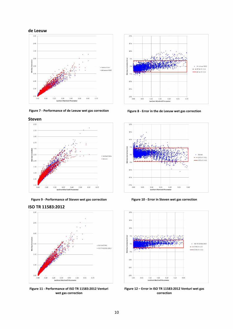
Figure 7, Figure 8 and Table 2 shows that the de Leeuw correlation is a better fit for this paper’s Venturi

data than any of the previous corrections, with a error of 3.829% (equivalent to an uncertainty of

3.673% to two standard deviations) for the bounded data. Figure 8 also shows that although the

error for this correlation has less bias than the previous corrections, there appears to be a positive bias at

larger liquid levels.

6

Steven

Richard Steven (formerly of NEL and Strathclyde University, now of CEESI and DP Diagnostics) wrote his

PhD[11] on Wet Gas Metering, including a new form of wet gas correction. This he further revised in a later

paper[12] to parameterise the A to D factors in terms of gas-to-liquid density ratio rather than pressure:

(19)

where:

(20)

The performance of this form of wet gas equation for the Venturi dataset can be seen (in Figure 9, Figure

10 and Table 2) to generally improve upon the Homogeneous and Orifice (Murdock, Chisholm, James, Lin,

Smith and Leang) wet gas corrections, but generally has greater error than the de Leeuw correction.

ISO TR 11583:2012

Emmelyn Graham and Michael Reader-Harris (both of TUV NEL) wrote a paper detailing a further wet gas

correction[13] before it later became part of a technical report for the International Organization for

Standardization[14]. In a similar manner to Chisholm and de Leeuw’s extensions of the Homogeneous

correction, the parameter from equation (16) is re-characterized to be:

(21)

H is a parameter depending on the type of liquid and its surface tensions (taken as 1.0 for hydrocarbon

liquid, 1.35 for water at ambient temperature, and 0.79 for liquid water in steam flow. Whilst this

parameter may be beneficial, its reliance on data that may not be readily known or measured in situ makes

this correction appear more arbitrary. However, as none of the Venturi data for this paper is for steam

flow, for the purposes of this paper only the following simplified equation for was used:

(22)

This standard also provides a correlation for the “discharge coefficient”:

(23)

This equation is elaborated upon in the paper[13], explaining that the initial value is “a remarkably close

approximation to the fitted value for the single-phase discharge coefficient, Cdry, which should apply both to

dry-gas flow and to homogeneous flow as Frgas,th tends to .” This is also true for the Venturi dataset

examined here, with an average dry gas discharge coefficient of 1.001, but implies that there may still be a

residual error at dry gas. For the purpose of the analysis given in this paper, is considered as an

7

additional part of the wet gas correction term. The performance of this correction is demonstrated in Table

2, Figure 11 and Figure 12, where this term corrects the initial negative bias seen in the error, further

reducing the wet gas correction errors. However, it is also noted that the paper[13] utilizes a slightly

different form for which improves the correlation (from 2.502% to 2.383% for ).

As an additional trial, the performance of the wet gas correction was evaluated for different values of .

The resulting data is given in Table 1, demonstrating that the correction is relatively insensitive to this

parameter, and therefore an assumption of water to liquid ratio

for the term only (which

results in ) provides an almost negligible change in the uncertainty given in this dataset.

However, the correct liquid density is still required for the rest of the correction term.

2δ relative wet gas correction uncertainty for ISO TR 11583:2012

All Data Points X <= 0.3 X <= 0.1

H calculated using actual WLR 2.584% 2.502% 2.338%

H calculated using WLR = 0.5 2.861% 2.744% 2.310%

H calculated using WLR = 0.0 2.624% 2.534% 2.335%

H calculated using WLR = 1.0 2.642% 2.569% 2.472%

Table 1 - Effect of changing H (via WLR) in ISO TR 11583:2012 Venturi wet gas correction

He and Bai

Denghui He and Bofeng Bai (from the State Key Laboratory of Multiphase Flow in Power Engineering, Xi’an

Jianotong University, China) have recently published a new wet gas correction based on a two-phase mass

flow coefficient [15]. The correction values are a correlation for a term based on extensive testing of two

Venturi flow meters (2” and 8”, Sch.80, ) over both two-phase and three-phase testing at CEESI:

(24)

Figure 13, Figure 14 and Table 2 shows that the performance of He and Bai’s correction over the Venturi

dataset for this paper is generally comparable to that of de Leeuw’s correction. However, as can be seen

from Figure 15, data with greater errors are generally concentrated at gas-to-liquid density ratios far in

excess of that seen by the correlation in the He and Bai paper, which had a maximum of 0.0441 for the 2”

and 0.081 for the 8” meter.

Manufacturer-Specific Wet Gas Correction

It is noted that various manufacturers of Venturi meters (including Solartron ISA) use “undisclosed wet gas

flow Venturi meter data sets and associated confidential correlations” ([16] section 6.4.3). The benefit of

this to the operator can be seen in Table 2 where a typical Solartron ISA wet gas correction correlated to

the data for each flow meter project has significantly improved performance over all other corrections

detailed in this paper.

Further graphical representation or equations for the Solartron ISA methods are not given in this as its

performance is solely provided as an example of a manufacturer-specific correction.

8

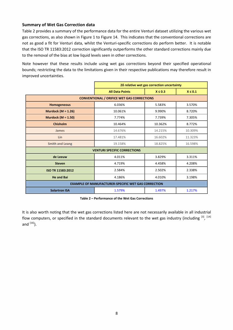
Summary of Wet Gas Correction data

Table 2 provides a summary of the performance data for the entire Venturi dataset utilizing the various wet

gas corrections, as also shown in Figure 1 to Figure 14. This indicates that the conventional corrections are

not as good a fit for Venturi data, whilst the Venturi-specific corrections do perform better. It is notable

that the ISO TR 11583:2012 correction significantly outperforms the other standard corrections mainly due

to the removal of the bias at low liquid levels seen in other corrections.

Note however that these results include using wet gas corrections beyond their specified operational

bounds; restricting the data to the limitations given in their respective publications may therefore result in

improved uncertainties.

2δ relative wet gas correction uncertainty

All Data Points X ≤ 0.3 X ≤ 0.1

CONVENTIONAL / ORIFICE WET GAS CORRECTIONS

Homogeneous 6.036% 5.583% 3.570%

Murdock (M = 1.26) 10.061% 9.990% 8.720%

Murdock (M = 1.50) 7.774% 7.739% 7.305%

Chisholm 10.464% 10.362% 8.772%

James 14.676% 14.215% 10.309%

Lin 17.481% 16.602% 11.323%

Smith and Leang 19.158% 18.825% 16.598%

VENTURI SPECIFIC CORRECTIONS

de Leeuw 4.011% 3.829% 3.311%

Steven 4.719% 4.458% 4.208%

ISO TR 11583:2012 2.584% 2.502% 2.338%

He and Bai 4.186% 4.010% 3.198%

EXAMPLE OF MANUFACTURER-SPECIFIC WET GAS CORRECTION

Solartron ISA 1.579% 1.497% 1.217%

Table 2 – Performance of the Wet Gas Corrections

It is also worth noting that the wet gas corrections listed here are not necessarily available in all industrial

flow computers, or specified in the standard documents relevant to the wet gas industry (including [3], [14]

and [16]).

9

Homogeneous

Figure 1 - Performance of the Homogeneous WGC

Figure 2 - Error in the Homogenous WGC

Murdock

Figure 3 - Murdock Wet Gas Correction, showing original and paper data

Figure 4 - Error in the Murdock (M = 1.50) WGC

Chisholm

Figure 5 – Performance of Chisholm wet gas correction

Figure 6 - Error in the Chisholm wet gas correction

10

de Leeuw

Figure 7 - Performance of de Leeuw wet gas correction

Figure 8 - Error in the de Leeuw wet gas correction

Steven

Figure 9 - Performance of Steven wet gas correction

Figure 10 - Error in Steven wet gas correction

ISO TR 11583:2012

Figure 11 - Performance of ISO TR 11583:2012 Venturi wet gas correction

Figure 12 – Error in ISO TR 11583:2012 Venturi wet gas correction

11

He and Bai

Figure 13 - Performance of He and Bai wet gas correction

Figure 14 – Error in He and Bai wet gas correction

Figure 15 – Error in He and Bai wet gas correction plotted against Density Ratio

12

IMPROVED CORRECTIONS Whilst the performance of the wet gas correction correlations in the previous section and Table 2

may be satisfactory for many applications, an additional benefit of the large Venturi dataset

available for this paper is to consider whether the flow measurement uncertainty can be reduced by

altering the value of parameters for the various correlations. As such, a randomized set containing

80% of the data (4,228 points) was used to update a number of the corrections by using Microsoft

Excel’s Solver routine (typically quadratic estimate, forward derivatives with conjugate search) to

optimise the selected parameters; the performance of the remaining 20% (1,057 test points) is then

shown separately to evaluate the performance of the improved correction.

For each wet gas correction, the parameters have been correlated for three different ranges of

points: all of the 80% data (i.e. 4,228 points), the 80% data where X < 0.3 (4,175 points), and the 80%

data where X < 0.1 (3,435 points). The tables given in the sections below list the parameter values,

the original correction performance (with a blue background), the performance for each optimised

region (white background), and the performance of the parameters correlated for the general wet

gas region (X < 0.3, shown with a green background) for the all data and X < 0.1 ranges.

“Improved” Murdock

The Murdock wet gas correction performance can be improved by altering the gradient ( in

equation (14)) to best fit the 80% data. However, as the correction is only a straight line, the

improvement seen to the 20% data between and is limited apart from for the

lower liquid level (low Lockhart Martinelli numbers) data, where the fitting procedure causes

significant changes to to attempt to correlate the initial curve in the Venturi data, as can be seen

in Figure 16 and Table 3.

2δ

80% 20%

M ALL DATA

Original 1.2600 10.006% 10.217%

Venturi Suggestion 1.5000 7.738% 7.877%

All Data Optimised 1.8128 6.397% 6.236%

X < 0.3 Optimised 1.8870 6.479% 6.221%

X < 0.3

Original 1.2600 9.936% 10.151%

Venturi Suggestion 1.5000 7.702% 7.850%

X < 0.3 Optimised 1.8870 5.922% 6.001%

X < 0.1

Original 1.2600 8.659% 8.964%

Venturi Suggestion 1.5000 7.255% 7.509%

X < 0.1 Optimised 2.3311 4.337% 4.425%

X < 0.3 Optimised 1.8870 5.336% 5.506%

Table 3 - Improved Murdock Correction Performance

As the benefits of fitting this dataset appear to be relatively small (i.e. still leaving significant

uncertainty) it is assumed that an improved “general” Murdock correction for all Venturi meters

should not to be implemented. A Murdock correction fitted for a specific Venturi meter may offer

13

some benefit, but other corrections described in this paper would better generally better suit a given

flow measurement application.

Figure 16 - Improved Murdock Correction

“Improved” Homogeneous or Chisholm

As both the homogenous and Chisholm corrections are identical except for the value of the

parameter, improvements to these two corrections can be considered together in a similar manner

to the parameter for the Murdock correction.

2δ

80% 20%

n ALL DATA

Chisholm 0.2500 10.439% 10.563%

Homogeneous 0.5000 6.005% 6.161%

All Data Optimised 0.4601 5.451% 5.519%

X < 0.3 Optimised 0.4692 5.479% 5.563%

X < 0.3

Chisholm 0.2500 10.322% 10.520%

Homogeneous 0.5000 5.493% 5.927%

X < 0.3 Optimised 0.4692 5.165% 5.431%

X < 0.1

Chisholm 0.2500 8.714% 9.001%

Homogeneous 0.5000 3.565% 3.590%

X < 0.1 Optimised 0.5245 3.402% 3.493%

X < 0.3 Optimised 0.4692 4.102% 4.110%

Table 4 - Improved Homogeneous or Chisholm Correction Performance

Table 4 demonstrates that fitting the parameter to the Venturi data provides only a small benefit

over the homogenous value, indicating the limitations of the form of this correction to match the

14

performance of the flow Venturi meter under wet gas conditions. Therefore a more complex

correction method may be required to provide better flow metering performance.

“Improved” de Leeuw

As the de Leeuw correction involves more parameters, for the purpose of this paper they are

characterised as:

(25)

Additionally we can relate these parameters when such that:

(26)

thus leaving only two free parameters to optimise. Optimising the value was also

considered and tested, but was found to offer very little additional benefit.

The parameters optimised for (i.e. the typical range for wet gas) show only a small

reduction in uncertainty from the original de Leeuw equation.

It is also worth noting the improvement shown between the improved homogeneous correction

(Figure 17) and the improved de Leeuw correction (Figure 18 – noting the difference in vertical axis

scale), where particularly at larger Lockhart-Martinelli numbers the scatter in the data is much

reduced. However, there is still a generally negative bias to the test points where .

2δ

80% 20%

AdL BdL CdL ALL DATA

Original 0.6060 -0.7460 0.4100 4.044% 3.875%

All Data Optimised 0.5731 -0.7918 0.3983 3.842% 3.706%

X < 0.3 Optimised 0.5736 -0.8245 0.4071 3.862% 3.729%

X < 0.3

Original 0.6060 -0.7460 0.4100 3.827% 3.837%

X < 0.3 Optimised 0.5736 -0.8245 0.4071 3.693% 3.703%

X < 0.1

Original 0.6060 -0.7460 0.4100 3.320% 3.275%

X < 0.1 Optimised 0.5800 -1.1127 0.4707 2.904% 2.970%

X < 0.3 Optimised 0.5736 -0.8245 0.4071 3.442% 3.384%

Table 5 - Improved de Leeuw Correction Parameters and Performance

Overall, there appears to be little benefit to “improving” the de Leeuw equation by optimising the

parameters to the larger Venturi dataset. It is therefore notable how well the original de Leeuw

equation works given the limited range of Venturi meters used in its development.

15

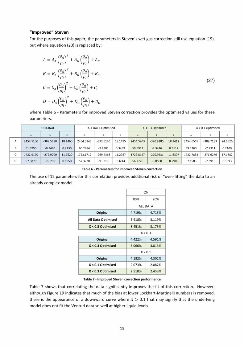
“Improved” Steven

For the purposes of this paper, the parameters in Steven’s wet gas correction still use equation (19),

but where equation (20) is replaced by:

(27)

where Table 6 - Parameters for improved Steven correction provides the optimised values for these

parameters.

ORIGINAL ALL DATA Optimised X < 0.3 Optimised X < 0.1 Optimised

A B C A B C A B C A B C

A 2454.5100 -389.5680 18.1460 2454.3343 -392.0140 18.1495 2454.5903 -390.9185 18.3412 2454.6565 -389.7183 24.6626

B 61.6950 -8.3490 0.2230 60.2484 -9.8381 0.3459 59.6912 -9.3426 0.3112 59.5260 -7.7311 0.2109

C 1722.9170 -272.9200 11.7520 1723.1712 -269.4366 11.2957 1722.8127 -270.9531 11.6307 1722.7832 -271.6276 17.1882

D 57.3870 -7.6790 0.1950 57.3220 -9.3315 0.3244 56.7776 -8.8500 0.2909 57.1583 -7.3915 0.1993

Table 6 - Parameters for improved Steven correction

The use of 12 parameters for this correlation provides additional risk of “over-fitting” the data to an

already complex model.

2δ

80% 20%

ALL DATA

Original 4.719% 4.713%

All Data Optimised 3.418% 3.119%

X < 0.3 Optimised 3.451% 3.175%

X < 0.3

Original 4.422% 4.591%

X < 0.3 Optimised 3.066% 3.015%

X < 0.1

Original 4.182% 4.302%

X < 0.1 Optimised 2.073% 2.082%

X < 0.3 Optimised 2.510% 2.453%

Table 7 - Improved Steven correction performance

Table 7 shows that correlating the data significantly improves the fit of this correction. However,

although Figure 19 indicates that much of the bias at lower Lockhart-Martinelli numbers is removed,

there is the appearance of a downward curve where that may signify that the underlying

model does not fit the Venturi data so well at higher liquid levels.

16

“Improved” ISO TR 11583:2012

For the purposes of this paper, the parameters in the ISO TR 11583:2012 paper Venturi wet gas

correction are characterised as:

(28)

(29)

By fully detailing the parameters for this correlation, the associated additional degrees of freedom

are made clear. As for the Steven correction, this increases the risk of over fitting the data, and a

simpler correction may be more parsimonious; however, the performance of this correlation may

justify the number of parameters.

Also, although and have the same value in the original correction, this is not assumed in

the “improved” parameters.

AISO BISO CISO DISO EISO FISO KISO LISO MISO NISO

Original 0.5830 -0.1800 -0.5780 -0.8000 0.3920 -0.1800 1.0000 -0.0463 -0.0500 0.0160

All Data Optimised 0.5211 0.0230 -0.4135 -0.6031 0.3421 -0.1797 1.0022 -0.0535 -0.0516 0.0116

X < 0.3 Optimised 0.5135 0.0475 -0.3999 -0.5901 0.3504 -0.1777 1.0023 -0.0524 -0.0499 0.0115

X < 0.1 Optimised 0.5479 0.0147 -0.3272 -0.5882 0.3223 -0.1863 1.0029 -0.0454 -0.0558 0.0053

Table 8 - Parameters for improved ISO TR 11583:2012 Venturi correction

2δ

80% 20%

ALL DATA

Original 2.608% 2.487%

All Data Optimised 2.407% 2.370%

X < 0.3 Optimised 2.410% 2.357%

X < 0.3

Original 2.509% 2.474%

X < 0.3 Optimised 2.379% 2.346%

X < 0.1

Original 2.352% 2.280%

X < 0.1 Optimised 2.198% 2.178%

X < 0.3 Optimised 2.313% 2.242%

Table 9 - Improved ISO TR 11583:2012 Venturi correction parameters and performance

As the ISO TR 11583:2012 already gave the best performance for the original wet gas corrections, it

is not surprising that the optimisation of the parameters generally gives only a small flow

measurement performance benefit. The scatter in the wet gas correction error seen in Figure 20

also shows the lack of bias due to the additional correlation parameters for low Lockhart-Martinelli

numbers.

17

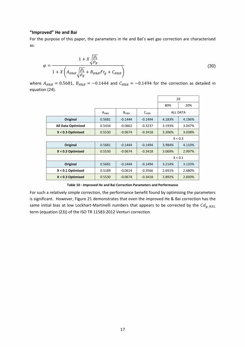
“Improved” He and Bai

For the purpose of this paper, the parameters in He and Bai’s wet gas correction are characterised

as:

(30)

where , and for the correction as detailed in

equation (24).

2δ

80% 20%

AH&B BH&B CH&B ALL DATA

Original 0.5681 -0.1444 -0.1494 4.183% 4.196%

All Data Optimised 0.5434 -0.0662 -0.3237 3.193% 3.047%

X < 0.3 Optimised 0.5530 -0.0674 -0.3418 3.206% 3.038%

X < 0.3

Original 0.5681 -0.1444 -0.1494 3.984% 4.110%

X < 0.3 Optimised 0.5530 -0.0674 -0.3418 3.069% 2.997%

X < 0.1

Original 0.5681 -0.1444 -0.1494 3.214% 3.133%

X < 0.1 Optimised 0.5189 -0.0614 -0.3566 2.691% 2.680%

X < 0.3 Optimised 0.5530 -0.0674 -0.3418 2.892% 2.830%

Table 10 - Improved He and Bai Correction Parameters and Performance

For such a relatively simple correction, the performance benefit found by optimising the parameters

is significant. However, Figure 21 demonstrates that even the improved He & Bai correction has the

same initial bias at low Lockhart-Martinelli numbers that appears to be corrected by the

term (equation (23)) of the ISO TR 11583:2012 Venturi correction.

18

Figure 17 - Improved Homogenous or Chisholm correction

Figure 18 - Improved de Leeuw correction

Figure 19 - Improved Steven correction

19

Figure 20 - Improved ISO TR 11583:2012

Figure 21 - Improved He & Bai correction

“Improved” Correction Discussion

The purpose of this section was to investigate whether the wet gas corrections could be improved by

simple adjustment of their parameters. Therefore Table 11 provides a summary of the performance

improvements for some of the wet gas corrections, alongside a count of the number of parameters

that were optimised.

2δ relative wet gas correction uncertainty

for X < 0.3 Optimised

Parameters Original "Improved" – 20% data

Murdock 7.739% (M=1.5) 6.001% 1

Homogeneous 5.583% 5.431% 1

de Leeuw 3.829% 3.703% 2

Steven 4.458% 3.015% 12

ISO TR 11583:2012 2.474% 2.346% 10

He and Bai 4.010% 2.997% 3

Table 11 - Summary of "Improved" Wet Gas Correction performance

20

The Murdock correction sees significant improvement, but it still has the greatest uncertainty of the

corrections considered in this section.

The Homogeneous/Chisholm correction is almost unimproved, but due to its curved form, it is a

better one parameter wet gas correction for Venturi meters than Murdock.

de Leeuw’s correction has only one additional free parameter when compared to

Murdock/Homogeneous/Chisholm, and it provides a significant improvement. However, as it is

almost unimproved by the correlation process and the effects of the parameter changes are small, it

would appear pertinent to continue to use the original parameter values.

The “improved” Steven and He & Bai have both similar performances and similar performance

improvements, despite a significant difference in the number of parameters to be optimised.

Further investigation and potential improvements of He and Bai’s correlation, particularly for higher

density ratios is recommended.

The ISO TR 11583:2012 correction continues to provide the best overall performance. It uses a

significant number of parameters, although its wet gas correction error performance may justify its

use. Again, as the effects of the parameter changes are small, it may be pertinent to continue to use

the original parameter values.

Although beyond the scope of this paper, it would also appear that the characteristics of the

transition between dry and wet gas flow for Venturi meters would also benefit from further

investigation in a comparable manner to from equation (23). Similarly, the effectiveness of

water-to-liquid (or similar) parameters in wet gas corrections, such as the use of in equation (21),

should be further considered.

CONCLUSIONS - The performance of a number of wet gas correction correlations has been evaluated for a large

Venturi dataset (see Table 2).

- The uncertainty of the wet gas corrections are generally increased for this dataset than those

stated in the relevant papers due to the far more extensive range of meters in this dataset.

- “Improved” corrections have been developed (using 80% of the dataset) and evaluated (using the

remaining 20% of the data). Only two (Steven and He & Bai) showed significant performance

benefits by optimising the parameters.

- Areas for further research into improving wet gas corrections should be considered, including

correlating terms at low Lockhart-Martinelli number and investigating the effects of water-to-liquid

ratio.

21

BIBLIOGRAPHY [1]. ISO 5167-4 Measurement of fluid flow by means of pressure differential devices inserted in

circular cross-section conduits running full - Part 4: Venturi tubes. 2003.

[2]. Wet Gas Flow Measurement in the Real World. One day seminar on Practical Developments in

Gas Flow Metering. Stobie, G., National Engineering Laboratory, East Kilbride, 1998.

[3]. ASME MFC-19G-2008 Wet Gas Flowmetering Guideline. 2008.

[4]. Venturi Meters and Wet Gas Flow. de Leeuw, Rick, Steven, Richard and van Maanen, Hans.,

North Sea Flow Measurement Workshop, 2011.

[5]. Two-Phase Flow Measurement with Orifices. Murdock, J.W. s.l. : Journal of Fluids Engineering,

1962, Vol. 84.4, pp. 419-432.

[6]. High Accuracy Wet Gas Metering. Jamieson, A.W and Dickinson, P.F. 1993. North Sea Flow

Measurement Workshop.

[7]. Research Note: Two-Phase Flow through Sharp-Edged Orifices. Chishom, D., Journal Mechanical

Engineering Science, 1977, Vol. 19 No.3.

[8]. Two-Phase Flow Measurement with Sharp-Edged Orifices. Lin, Z.H. s.l. : Int. J. Multiphase Flow,

1982, Vols. 8, No.6, pp. 683-693.

[9]. Metering of Steam-Water Two-Phase Flow by Sharp-Edged Orifices. James, Russell., Proc. Instn.

Mech. Engrs, 1965, Vols. 180, Pt.1, No.23.

[10]. Evaluations of Correlations for Two-Phase Flowmeters Three Current-One New. Smith, R. V. and

Leang, J. T., Journal of Engineering for Gas Turbines and Power, 1975, Vol. 97, pp. 589-593.

[11]. Wet Gas Metering. Steven, R.N., PhD Thesis, University of Strathclyde, 2001.

[12]. Wet gas metering with a horizontally mounted Venturi meter. Steven, R.N., Flow Measurement

and Instrumentation, 2002, Vol. 12, pp. 361-372.

[13]. Venturi Tubes in Wet Gas - Improved Models for the Over-Reading and the Pressure-Loss Ratio

Method. Graham, Emmelyn and Reader-Harris, Michael., SE Asia Hydrocarbon Flow Measurement

Workshop, 2010.

[14]. PD ISO/TR 11583:2012 Measurement of wet gas flow by means of pressure differential devices

inserted in circular cross-section conduits.

[15]. A new correlation for wet gas flow rate measurement with Venturi meter based on two-phase

mass flow coefficient. He, Denghui and Bai, Bofeng., Measurement, 2014, Vol. 58, pp. 61-67.

[16]. ISO/TR 12748 Measurement of wet natural gas flow in circular cross-section conduits. 2015.

[17]. Liquid Correction of Venturi Meter Readings in Wet Gas Flow. de Leeuw, Rick., North Sea Flow

Measurement Workshop, 1997.

[18]. Evolution of Wet Gas Venturi Metering and Wet Gas Correction Algorithms. Collins, Alistair and

Clark, Steve. 1 February 2013, Vol. 46, pp. 15-20.