Economic Value Added (EVA) and the Valuation of Small Businesses

by Michael F. Spivey Department of Finance College of Business and Public Affairs Clemson University

Jeffrey J. McMillan School of Accountancy & Legal Studies

College Business and Public Affairs Clemson University

Abstract: This article first provides an overview of the standard asset, market, and income valuation methods that are generally used to estimate the value of small businesses. It then discusses economic value added (EVA) and demonstrates its potential use in the valuation of small businesses.

1

Economic Value Added (EVA) and the Valuation of Small Businesses 1. Introduction

Market valuation and shareholder value creation has become an increasingly important issue for

businesses. Financial statements reporting book values do not reflect the true financial condition of most

businesses; thus, value estimation plays a vital role in the business community. Any financial endeavor,

such as attracting new investors or making investment decisions, necessitates the consideration of the

equity value created by the endeavor. This is particularly true for many entrepreneurial and small

businesses that often need to finance high growth and attract capital from outside investors.

A major problem of market valuation of many entrepreneurial types of businesses is that their

equity is not traded in broad, public markets. Most entrepreneurial businesses are relatively small and

are either privately owned or are publicly traded in very thin secondary markets. Subsequently market

assessment of the true value of the firm’s equity is not readily available. Consequently, having a

background and a better understanding of the alternative concepts and techniques that may be used to

estimate the value of businesses that are not actively traded can help entrepreneurs/management better

plan and manage their businesses.

After reading the article small business owners should feel more comfortable talking with

accounting/financial individuals about how their business might be valued and also thinking about how

actions they are currently taking (or may take) could possibly affect the value of their business. In the

life of a small business, undoubtedly circumstances will arise where entrepreneurs (owners) or

management will find familiarity with valuation concepts useful (e.g., when seeking new capital, going

public, during merger situations, or the selling of the business). This paper provides an

2

overview of traditional methods utilized in the valuation of closely-held businesses.1 It then discusses the

application of economic value added (EVA) in the valuation of closely-held businesses. EVA, along

with market value added (MVA), is a more recent financial performance measure and has received

some much-heralded support. CS First Boston, for example, utilizes EVA to assess corporate

performance and to value equity securities.2 EVA has also been used to help assess value creation in

the nonprofit sector.3

2. Traditional Approaches of Valuation

This section of the paper reviews the three most common approaches used to value closely-held

businesses, the asset method, the market method, and the income method. There is no exact formula

that can be used to evaluate every type of closely-held business; therefore, the equity of a particular

business can be valued differently by different methods. Several factors may be considered in valuing a

closely-held stock and use of these factors is quite subjective. One factor to consider in valuing a

closely-held stock is the price of publicly-traded stocks engaged in the same or similar lines of business.

Another factor to consider is the nature of the business and its prior history. The company’s growth

history and its diversity of operations allow one to form an opinion on the degree of risk involved in the

business. Areas of particular interest when evaluating the industry and a company's prior history are

past gross income, net income, and the dividend payout over long time periods, preferably five or more

years. Financial information such as liquidity measures, fixed assets, working capital, long-term liability,

and net worth are also important. The economic outlook for a closely-held company should also be

1 Small, privately-held and closely-held will be used interchangeably throughout the paper. 2See Jackson (1996). 3 See Gapenski (1996).

3

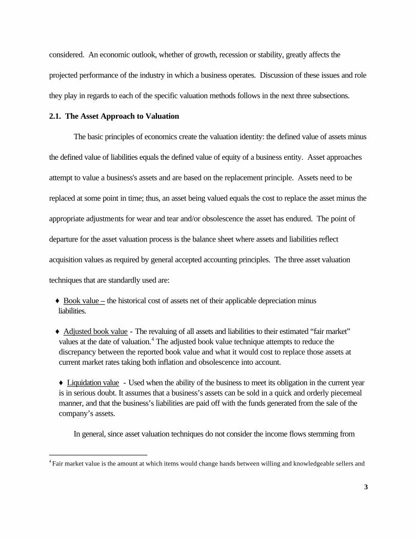
considered. An economic outlook, whether of growth, recession or stability, greatly affects the

projected performance of the industry in which a business operates. Discussion of these issues and role

they play in regards to each of the specific valuation methods follows in the next three subsections.

2.1. The Asset Approach to Valuation

The basic principles of economics create the valuation identity: the defined value of assets minus

the defined value of liabilities equals the defined value of equity of a business entity. Asset approaches

attempt to value a business's assets and are based on the replacement principle. Assets need to be

replaced at some point in time; thus, an asset being valued equals the cost to replace the asset minus the

appropriate adjustments for wear and tear and/or obsolescence the asset has endured. The point of

departure for the asset valuation process is the balance sheet where assets and liabilities reflect

acquisition values as required by general accepted accounting principles. The three asset valuation

techniques that are standardly used are:

♦ Book value – the historical cost of assets net of their applicable depreciation minus liabilities.

♦ Adjusted book value - The revaluing of all assets and liabilities to their estimated “fair market”

values at the date of valuation.4 The adjusted book value technique attempts to reduce the discrepancy between the reported book value and what it would cost to replace those assets at current market rates taking both inflation and obsolescence into account.

♦ Liquidation value - Used when the ability of the business to meet its obligation in the current year is in serious doubt. It assumes that a business’s assets can be sold in a quick and orderly piecemeal manner, and that the business’s liabilities are paid off with the funds generated from the sale of the company’s assets.

In general, since asset valuation techniques do not consider the income flows stemming from

4 Fair market value is the amount at which items would change hands between willing and knowledgeable sellers and

4

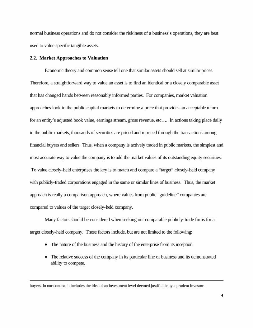
normal business operations and do not consider the riskiness of a business’s operations, they are best

used to value specific tangible assets.

2.2. Market Approaches to Valuation

Economic theory and common sense tell one that similar assets should sell at similar prices.

Therefore, a straightforward way to value an asset is to find an identical or a closely comparable asset

that has changed hands between reasonably informed parties. For companies, market valuation

approaches look to the public capital markets to determine a price that provides an acceptable return

for an entity’s adjusted book value, earnings stream, gross revenue, etc…. In actions taking place daily

in the public markets, thousands of securities are priced and repriced through the transactions among

financial buyers and sellers. Thus, when a company is actively traded in public markets, the simplest and

most accurate way to value the company is to add the market values of its outstanding equity securities.

To value closely-held enterprises the key is to match and compare a “target” closely-held company

with publicly-traded corporations engaged in the same or similar lines of business. Thus, the market

approach is really a comparison approach, where values from public “guideline” companies are

compared to values of the target closely-held company.

Many factors should be considered when seeking out comparable publicly-trade firms for a

target closely-held company. These factors include, but are not limited to the following:

♦ The nature of the business and the history of the enterprise from its inception.

♦ The relative success of the company in its particular line of business and its demonstrated ability to compete.

buyers. In our context, it includes the idea of an investment level deemed justifiable by a prudent investor.

5

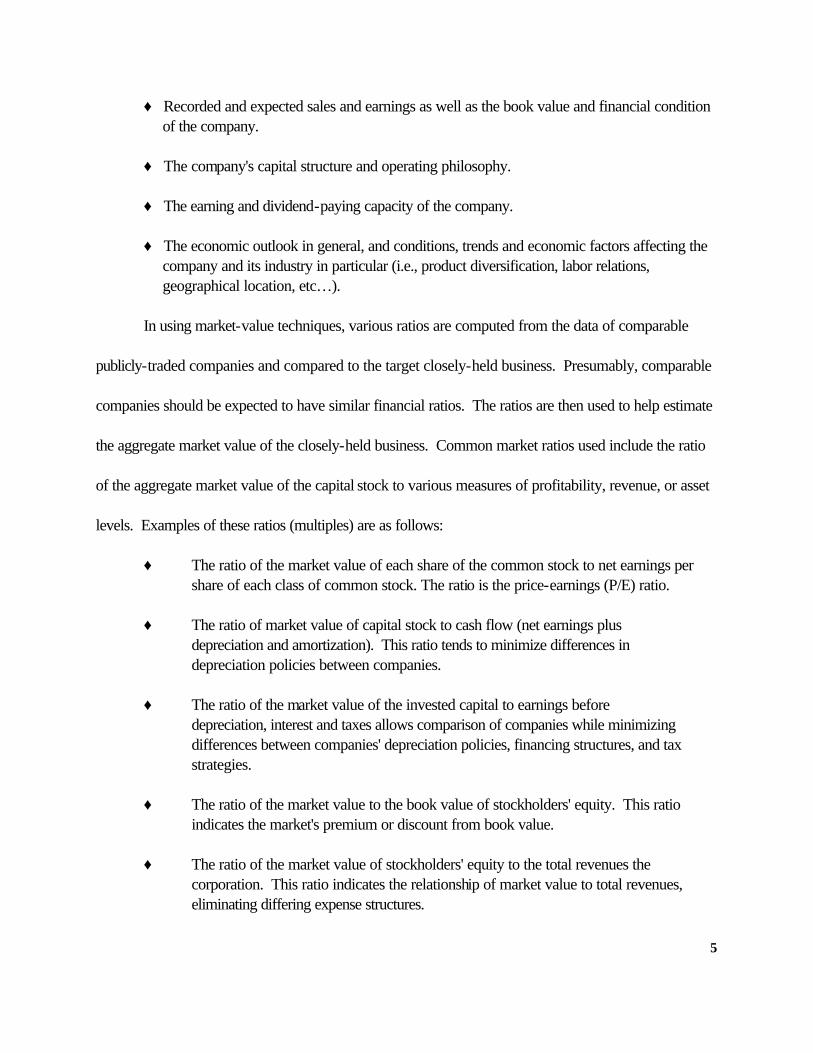
♦ Recorded and expected sales and earnings as well as the book value and financial condition of the company.

♦ The company's capital structure and operating philosophy.

♦ The earning and dividend-paying capacity of the company.

♦ The economic outlook in general, and conditions, trends and economic factors affecting the

company and its industry in particular (i.e., product diversification, labor relations, geographical location, etc…).

In using market-value techniques, various ratios are computed from the data of comparable

publicly-traded companies and compared to the target closely-held business. Presumably, comparable

companies should be expected to have similar financial ratios. The ratios are then used to help estimate

the aggregate market value of the closely-held business. Common market ratios used include the ratio

of the aggregate market value of the capital stock to various measures of profitability, revenue, or asset

levels. Examples of these ratios (multiples) are as follows:

♦ The ratio of the market value of each share of the common stock to net earnings per share of each class of common stock. The ratio is the price-earnings (P/E) ratio.

♦ The ratio of market value of capital stock to cash flow (net earnings plus depreciation and amortization). This ratio tends to minimize differences in

depreciation policies between companies.

♦ The ratio of the market value of the invested capital to earnings before depreciation, interest and taxes allows comparison of companies while minimizing differences between companies' depreciation policies, financing structures, and tax strategies.

♦ The ratio of the market value to the book value of stockholders' equity. This ratio

indicates the market's premium or discount from book value.

♦ The ratio of the market value of stockholders' equity to the total revenues the corporation. This ratio indicates the relationship of market value to total revenues, eliminating differing expense structures.

6

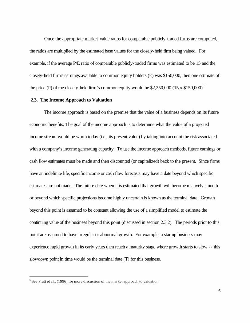
Once the appropriate market-value ratios for comparable publicly-traded firms are computed,

the ratios are multiplied by the estimated base values for the closely-held firm being valued. For

example, if the average P/E ratio of comparable publicly-traded firms was estimated to be 15 and the

closely-held firm's earnings available to common equity holders (E) was $150,000, then one estimate of

the price (P) of the closely-held firm’s common equity would be $2,250,000 (15 x $150,000).5

2.3. The Income Approach to Valuation

The income approach is based on the premise that the value of a business depends on its future

economic benefits. The goal of the income approach is to determine what the value of a projected

income stream would be worth today (i.e., its present value) by taking into account the risk associated

with a company’s income generating capacity. To use the income approach methods, future earnings or

cash flow estimates must be made and then discounted (or capitalized) back to the present. Since firms

have an indefinite life, specific income or cash flow forecasts may have a date beyond which specific

estimates are not made. The future date when it is estimated that growth will become relatively smooth

or beyond which specific projections become highly uncertain is known as the terminal date. Growth

beyond this point is assumed to be constant allowing the use of a simplified model to estimate the

continuing value of the business beyond this point (discussed in section 2.3.2). The periods prior to this

point are assumed to have irregular or abnormal growth. For example, a startup business may

experience rapid growth in its early years then reach a maturity stage where growth starts to slow -- this

slowdown point in time would be the terminal date (T) for this business.

5 See Pratt et al., (1996) for more discussion of the market approach to valuation.

7

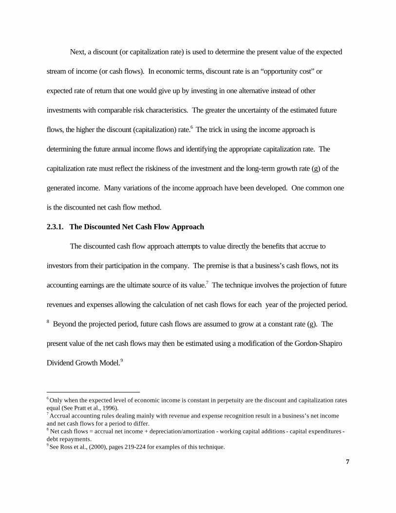
Next, a discount (or capitalization rate) is used to determine the present value of the expected

stream of income (or cash flows). In economic terms, discount rate is an “opportunity cost” or

expected rate of return that one would give up by investing in one alternative instead of other

investments with comparable risk characteristics. The greater the uncertainty of the estimated future

flows, the higher the discount (capitalization) rate.6 The trick in using the income approach is

determining the future annual income flows and identifying the appropriate capitalization rate. The

capitalization rate must reflect the riskiness of the investment and the long-term growth rate (g) of the

generated income. Many variations of the income approach have been developed. One common one

is the discounted net cash flow method.

2.3.1. The Discounted Net Cash Flow Approach

The discounted cash flow approach attempts to value directly the benefits that accrue to

investors from their participation in the company. The premise is that a business’s cash flows, not its

accounting earnings are the ultimate source of its value.7 The technique involves the projection of future

revenues and expenses allowing the calculation of net cash flows for each year of the projected period.

8 Beyond the projected period, future cash flows are assumed to grow at a constant rate (g). The

present value of the net cash flows may then be estimated using a modification of the Gordon-Shapiro

Dividend Growth Model.9

6 Only when the expected level of economic income is constant in perpetuity are the discount and capitalization rates equal (See Pratt et al., 1996). 7 Accrual accounting rules dealing mainly with revenue and expense recognition result in a business’s net income and net cash flows for a period to differ. 8 Net cash flows = accrual net income + depreciation/amortization - working capital additions - capital expenditures - debt repayments. 9 See Ross et al., (2000), pages 219-224 for examples of this technique.

8

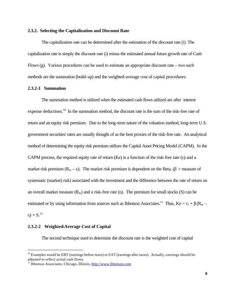
2.3.2. Selecting the Capitalization and Discount Rate

The capitalization rate can be determined after the estimation of the discount rate (i). The

capitalization rate is simply the discount rate (i) minus the estimated annual future growth rate of Cash

Flows (g). Various procedures can be used to estimate an appropriate discount rate – two such

methods are the summation (build-up) and the weighted-average cost of capital procedures.

2.3.2-1 Summation

The summation method is utilized when the estimated cash flows utilized are after interest

expense deductions.10 In the summation method, the discount rate is the sum of the risk-free rate of

return and an equity risk premium. Due to the long-term nature of the valuation method, long-term U.S.

government securities' rates are usually thought of as the best proxies of the risk-free rate. An analytical

method of determining the equity risk premium utilizes the Capital Asset Pricing Model (CAPM). In the

CAPM process, the required equity rate of return (Ke) is a function of the risk-free rate (rf) and a

market risk premium (Rm – rf). The market risk premium is dependent on the Beta, (β = measure of

systematic (market) risk) associated with the investment and the difference between the rate of return on

an overall market measure (Rm) and a risk-free rate (rf). The premium for small stocks (S) can be

estimated or by using information from sources such as Ibbotson Associates.11 Thus, Ke = rf + β(Rm –

rf) + S.12

2.3.2-2 Weighted-Average Cost of Capital

The second technique used to determine the discount rate is the weighted cost of capital

10 Examples would be EBT (earnings before taxes) or EAT (earnings after taxes). Actually, earnings should be adjusted to reflect actual cash flows. 11 Ibbotson Associates, Chicago, Illinois, http://www.ibbotson.com

9

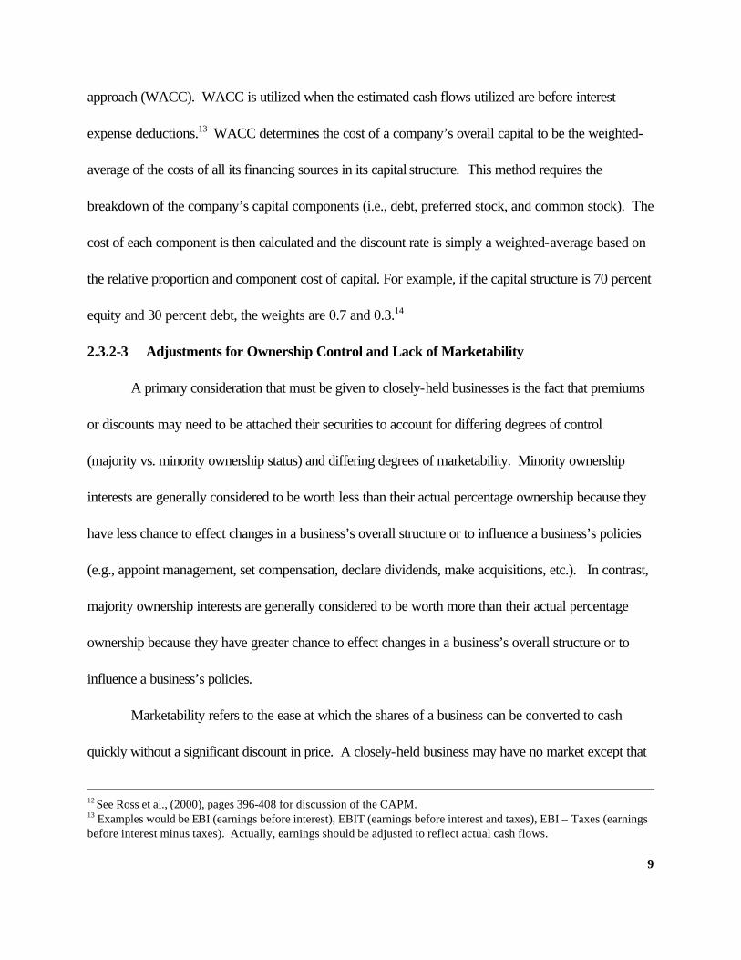
approach (WACC). WACC is utilized when the estimated cash flows utilized are before interest

expense deductions.13 WACC determines the cost of a company’s overall capital to be the weighted-

average of the costs of all its financing sources in its capital structure. This method requires the

breakdown of the company’s capital components (i.e., debt, preferred stock, and common stock). The

cost of each component is then calculated and the discount rate is simply a weighted-average based on

the relative proportion and component cost of capital. For example, if the capital structure is 70 percent

equity and 30 percent debt, the weights are 0.7 and 0.3.14

2.3.2-3 Adjustments for Ownership Control and Lack of Marketability

A primary consideration that must be given to closely-held businesses is the fact that premiums

or discounts may need to be attached their securities to account for differing degrees of control

(majority vs. minority ownership status) and differing degrees of marketability. Minority ownership

interests are generally considered to be worth less than their actual percentage ownership because they

have less chance to effect changes in a business’s overall structure or to influence a business’s policies

(e.g., appoint management, set compensation, declare dividends, make acquisitions, etc.). In contrast,

majority ownership interests are generally considered to be worth more than their actual percentage

ownership because they have greater chance to effect changes in a business’s overall structure or to

influence a business’s policies.

Marketability refers to the ease at which the shares of a business can be converted to cash

quickly without a significant discount in price. A closely-held business may have no market except that

12 See Ross et al., (2000), pages 396-408 for discussion of the CAPM. 13 Examples would be EBI (earnings before interest), EBIT (earnings before interest and taxes), EBI – Taxes (earnings before interest minus taxes). Actually, earnings should be adjusted to reflect actual cash flows.

10

market created by an aggressive seller actively seeking prospective buyers. Thus, investment risk is

much higher for closely-held investments than for investments with active secondary markets.15

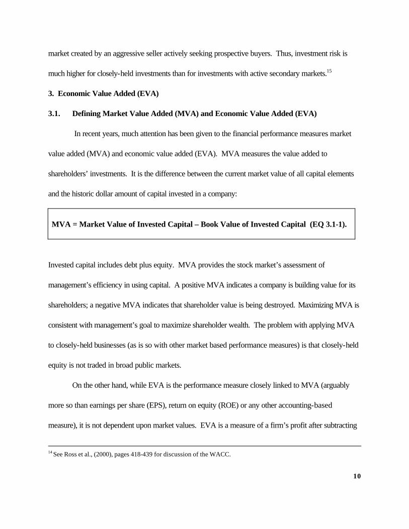
3. Economic Value Added (EVA)

3.1. Defining Market Value Added (MVA) and Economic Value Added (EVA)

In recent years, much attention has been given to the financial performance measures market

value added (MVA) and economic value added (EVA). MVA measures the value added to

shareholders’ investments. It is the difference between the current market value of all capital elements

and the historic dollar amount of capital invested in a company:

MVA = Market Value of Invested Capital – Book Value of Invested Capital (EQ 3.1-1).

Invested capital includes debt plus equity. MVA provides the stock market’s assessment of

management’s efficiency in using capital. A positive MVA indicates a company is building value for its

shareholders; a negative MVA indicates that shareholder value is being destroyed. Maximizing MVA is

consistent with management’s goal to maximize shareholder wealth. The problem with applying MVA

to closely-held businesses (as is so with other market based performance measures) is that closely-held

equity is not traded in broad public markets.

On the other hand, while EVA is the performance measure closely linked to MVA (arguably

more so than earnings per share (EPS), return on equity (ROE) or any other accounting-based

measure), it is not dependent upon market values. EVA is a measure of a firm’s profit after subtracting

14 See Ross et al., (2000), pages 418-439 for discussion of the WACC.

11

the cost of all capital employed (debt + equity). EVA has been viewed as a tool to help evaluate the

operating performance of businesses or of specific operating departments within businesses. Since it is

not based on the market, it may have significant use as a technique for valuing closely-held businesses.

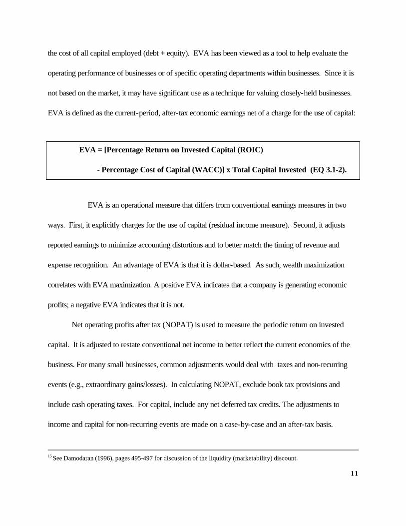
EVA is defined as the current-period, after-tax economic earnings net of a charge for the use of capital:

EVA is an operational measure that differs from conventional earnings measures in two

ways. First, it explicitly charges for the use of capital (residual income measure). Second, it adjusts

reported earnings to minimize accounting distortions and to better match the timing of revenue and

expense recognition. An advantage of EVA is that it is dollar-based. As such, wealth maximization

correlates with EVA maximization. A positive EVA indicates that a company is generating economic

profits; a negative EVA indicates that it is not.

Net operating profits after tax (NOPAT) is used to measure the periodic return on invested

capital. It is adjusted to restate conventional net income to better reflect the current economics of the

business. For many small businesses, common adjustments would deal with taxes and non-recurring

events (e.g., extraordinary gains/losses). In calculating NOPAT, exclude book tax provisions and

include cash operating taxes. For capital, include any net deferred tax credits. The adjustments to

income and capital for non-recurring events are made on a case-by-case and an after-tax basis.

15 See Damodaran (1996), pages 495-497 for discussion of the liquidity (marketability) discount.

EVA = [Percentage Return on Invested Capital (ROIC)

- Percentage Cost of Capital (WACC)] x Total Capital Invested (EQ 3.1-2).

12

The capital charge (Percentage Cost of Capital x Capital Invested) covers not only interest

charges on debt but also a return that adequately compensates for the riskiness of the

equity investment. This converts the balance sheet into another expense (capital costs) that may be

compared directly with and managed in the same way as normal operating expenses. In practice, the

weighted-average cost of capital (WACC) is frequently utilized as a measure of the percentage cost of

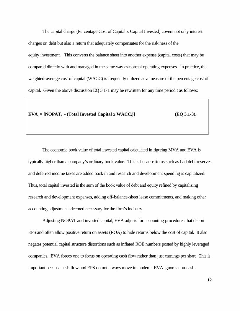
capital. Given the above discussion EQ 3.1-1 may be rewritten for any time period t as follows:

EVAt = [NOPATt - (Total Invested Capital x WACCt)] (EQ 3.1-3).

The economic book value of total invested capital calculated in figuring MVA and EVA is

typically higher than a company’s ordinary book value. This is because items such as bad debt reserves

and deferred income taxes are added back in and research and development spending is capitalized.

Thus, total capital invested is the sum of the book value of debt and equity refined by capitalizing

research and development expenses, adding off-balance-sheet lease commitments, and making other

accounting adjustments deemed necessary for the firm’s industry.

Adjusting NOPAT and invested capital, EVA adjusts for accounting procedures that distort

EPS and often allow positive return on assets (ROA) to hide returns below the cost of capital. It also

negates potential capital structure distortions such as inflated ROE numbers posted by highly leveraged

companies. EVA forces one to focus on operating cash flow rather than just earnings per share. This is

important because cash flow and EPS do not always move in tandem. EVA ignores non-cash

13

accounting charges and asks the right question, “is an acceptable return on investment being made.” In

addition to the general failure of EPS and price/multiples ability to capture the reality of cash flows, they

do not capture specific and systematic risk levels among companies, or the differences in expected cash

flow timings or length of the cash flow periods. On the other hand, EVA allows one to answer the

question: What are the levels of future cash flows, rates of return, and length of the competitive

advantage period necessary to justify today’s stock price?

Companies can bolster EPS growth simply by retaining more earnings and raising more capital.

The market appreciates increased cash generation while employing less capital and this is where EVA

steps in as it focuses on after-tax cash flow instead of EPS. It encourages improving operating profits

without using more capital, the investing of capital in projects that earn more than the cost of capital (i.e.,

a positive ROIC-WACC spread), and eliminating investment in operations where returns are

inadequate. Thus, within large organizations, EVA can be used to determine whether economic profits

from one division are subsidizing a less profitable division or can be used to help identify bargains, or

temporary market underpricings.

3. 2. EVA as a Valuation Tool

EVA may be viewed as an extension of the income approach to valuation. Subsequently, it

recognizes that the value of a business depends on its future economic benefits. With EVA, estimates of

key factors that determine future earnings or cash flows must be made. These factors include such

variables as unit volume growth, operating margins, the cost of capital, and the expected levels of

adjusted NOPAT and invested capital. As covered in our discussion of the income approach, a

terminal date (T) when growth is assumed to become relatively smooth and predictable may need to be

14

estimated. If this terminal date follows a period of higher than expected growth, then the level of

abnormal growth and its duration must be estimated. The choice of a particular period of abnormal

growth is subjective in nature but should consider factors such as the proprietary nature of technologies,

patent protection, the value of branded good franchises and access to distribution channels.

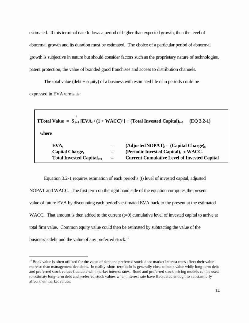
The total value (debt + equity) of a business with estimated life of n periods could be expressed in EVA terms as:

Equation 3.2-1 requires estimation of each period’s (t) level of invested capital, adjusted

NOPAT and WACC. The first term on the right hand side of the equation computes the present

value of future EVA by discounting each period’s estimated EVA back to the present at the estimated

WACC. That amount is then added to the current (t=0) cumulative level of invested capital to arrive at

total firm value. Common equity value could then be estimated by subtracting the value of the

business’s debt and the value of any preferred stock.16

16 Book value is often utilized for the value of debt and preferred stock since market interest rates affect their value more so than management decisions. In reality, short-term debt is generally close to book value while long-term debt and preferred stock values fluctuate with market interest rates. Bond and preferred stock pricing models can be used to estimate long-term debt and preferred stock values when interest rate have fluctuated enough to substantially affect their market values.

n

TTotal Value = Σ t=1 [EVAt / (1 + WACC)t ] + (Total Invested Capital)t=0 (EQ 3.2-1) where EVAt = (Adjusted NOPAT)t – (Capital Charge)t, Capital Charget = (Periodic Invested Capital)t x WACC. Total Invested Capitalt=0 = Current Cumulative Level of Invested Capital

15

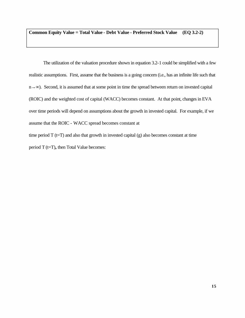
Common Equity Value = Total Value - Debt Value - Preferred Stock Value (EQ 3.2-2)

The utilization of the valuation procedure shown in equation 3.2-1 could be simplified with a few

realistic assumptions. First, assume that the business is a going concern (i.e., has an infinite life such that

n→∞). Second, it is assumed that at some point in time the spread between return on invested capital

(ROIC) and the weighted cost of capital (WACC) becomes constant. At that point, changes in EVA

over time periods will depend on assumptions about the growth in invested capital. For example, if we

assume that the ROIC - WACC spread becomes constant at

time period T (t=T) and also that growth in invested capital (g) also becomes constant at time period T (t=T), then Total Value becomes:

16

T

Total Value = Σ t=1 [EVAt / (1 + WACC)t ] +

{[EVAt=T x (1 + g)] / (WACC - g)} / (1 + WACC)T +

(Total Invested Capital)t=0 (EQ 3.2-3)

17

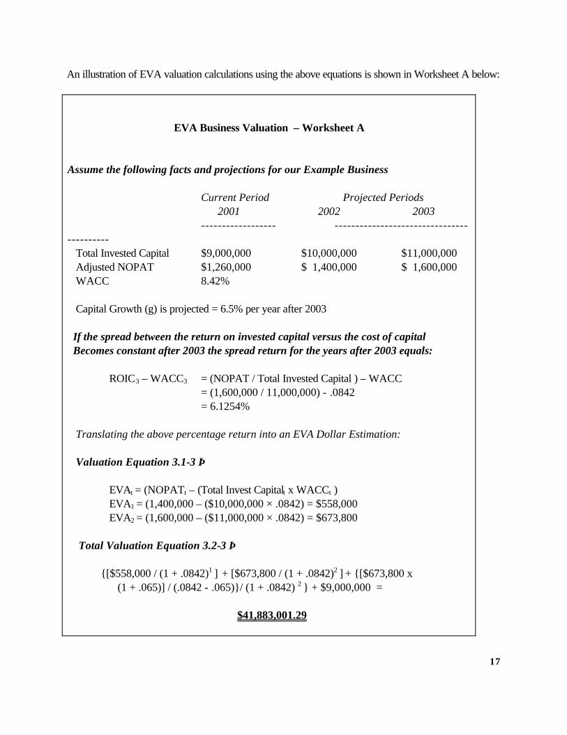
An illustration of EVA valuation calculations using the above equations is shown in Worksheet A below:

EVA Business Valuation – Worksheet A

Assume the following facts and projections for our Example Business

Current Period Projected Periods 2001 2002 2003 ------------------ ------------------------------------------ Total Invested Capital $9,000,000 $10,000,000 $11,000,000 Adjusted NOPAT $1,260,000 $ 1,400,000 $ 1,600,000 WACC 8.42% Capital Growth (g) is projected = 6.5% per year after 2003 If the spread between the return on invested capital versus the cost of capital Becomes constant after 2003 the spread return for the years after 2003 equals: ROIC3 – WACC3 = (NOPAT / Total Invested Capital ) – WACC = (1,600,000 / 11,000,000) - .0842 = 6.1254% Translating the above percentage return into an EVA Dollar Estimation: Valuation Equation 3.1-3 ⇒ EVAt = (NOPATt – (Total Invest Capitalt x WACCt ) EVA1 = (1,400,000 – ($10,000,000 × .0842) = $558,000 EVA2 = (1,600,000 – ($11,000,000 × .0842) = $673,800 Total Valuation Equation 3.2-3 ⇒ {[$558,000 / (1 + .0842)1 ]

+ [$673,800 / (1 + .0842)2 ] + {[$673,800 x

(1 + .065)] / (.0842 - .065)}/ (1 + .0842) 2 } + $9,000,000 = $41,883,001.29

18

19

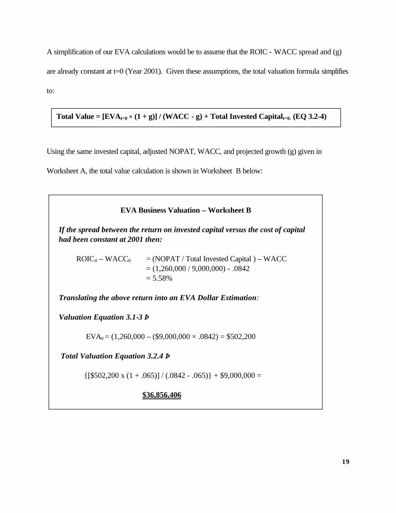
A simplification of our EVA calculations would be to assume that the ROIC - WACC spread and (g)

are already constant at t=0 (Year 2001). Given these assumptions, the total valuation formula simplifies

to:

Using the same invested capital, adjusted NOPAT, WACC, and projected growth (g) given in

Worksheet A, the total value calculation is shown in Worksheet B below:

EVA Business Valuation – Worksheet B If the spread between the return on invested capital versus the cost of capital had been constant at 2001 then: ROIC0 – WACC0 = (NOPAT / Total Invested Capital ) – WACC = (1,260,000 / 9,000,000) - .0842 = 5.58% Translating the above return into an EVA Dollar Estimation: Valuation Equation 3.1-3 ⇒ EVA0 = (1,260,000 – ($9,000,000 × .0842) = $502,200 Total Valuation Equation 3.2.4 ⇒ {[$502,200 x (1 + .065)] / (.0842 - .065)} + $9,000,000 = $36,856,406

Total Value = [EVAt=0 × (1 + g)] / (WACC - g) + Total Invested Capitalt=0. (EQ 3.2-4)

20

As can be seen, the valuation models can be quite sensitive to changes in assumptions. Worksheet A

circumstances resulted in a valuation approximately 12 percent greater than the valuation estimated in

Worksheet B ($41,883,000 versus $36,856,406). This was due to the lowered growth estimates for

years 1 and 2. Sensitivity analysis could be employed to examine the effect of other key inputs (such as

the WACC) on estimated value.

4. Conclusion This article provides an overview of the standard asset, market, and income valuation methods.

It then discusses the concepts associated with EVA and demonstrates it as an extension of the income

approach for valuing small businesses. EVA is a periodic performance measure that allows one to

assess how “value” has been added to the business through its normal operations each accounting

period. Although cash-oriented, EVA begins with a business’ after-tax net operating earnings, then

adjusts for distortions of cash flow by accounting conventions and takes into account the capital charge

that is necessary to compensate shareholders for the riskiness of their investments.

21

Bibliography

Damodaran, Aswath, 1996, Investment Valuation, John Wiley and Sons, Inc. Copeland, T., T. Koller and J. Murrin, 1998, Valuation: Measuring and managing the Value of Companies, 2nd edition, John Wiley and Sons, Inc. Gapenski, Louis C., 1996, “Using MVA and EVA to Measure Financial Performance,” Healthcare Financial Management, Volume 50(March), pp. 56-60. Grant, James L., 1996, “Foundations of EVA for Investment Managers,” Journal of Portfolio Management, Fall, pp. 41-48. Jackson, Alfred, 1996, “The How and Why of EVA at CS First Boston,” Journal of Applied Corporate Finance, Volume 9 Number 1, Spring, pp. 98-103. O’Byrne, Stephen F., 1996, ”EVA and Market Value,” Journal of Applied Corporate Finance, Volume 9 Number 1, Spring, pp. 116-125. Pratt, Shannon P., Reilly, Robert F. and Robert P. Schweihs, 1996, Valuing a Business: The Analysis and Appraisal of Closely Held Companies, 3rd edition, Homewood, Illinois, Irwin. Ross, S., R. Westerfield and B. Jordan, 2000, Fundamentals of Corporate Finance, 5th edition, Irwin McGraw-Hill, Inc. Stern, Joel M., Stewart III, G. Bennett and Donald H. Chew Jr. , 1995, “The EVA Financial Management System,” Journal of Applied Corporate Finance, Volume 8, Number 2, pp. 32-46. Stewart III, G. Bennett, 1990, “Announcing the Stern Stewart Performance 1,000: A New Way of Viewing Corporate America”, Journal of Applied Corporate Finance, Volume 3, Number 2, pp. 38-59. Uyemura, D.G., C.C. Kantor, and J.M. Pettit, 1996, “EVA For Banks: Value Creation, Risk Management, and Profitability Measurement,” Journal of Applied Corporate Finance, Volume 9, Number 2, pp. 94-113.