EUROPEAN JOURNAL RESEARCH ELSEVIER Theory … strategic/elsvier/el537.pdf · Theory and Methodology A procedure for optimizing tactical response in oil spill clean up ... tactical

EUROPEAN JOURNAL

OF OPERATIONAL RESEARCH

ELSEVIER European Journal of Operational Research 102 (1997) 554-574

Theory and Methodology

A procedure for optimizing tactical response in oil spill clean up operations

Anand V. Srinivasa a Wilbert E. Wilhelm b,*

a i2 Technologies, 909 East Las Colinas Blvd., 16th Floor, Irving, TX 75039, USA b Department of Industrial Engineering, Texas A &M University, College Station, TX 77843-3131, USA

Received 24 May 1995; revised 27 June 1996

Abstract

The Tactical Decision Problem (TDP) associated with oil spill clean up operations allocates available components to compose response systems so that the clean up requirement for each time period over the entire planning horizon is met. The objective is to minimize total response time to allow for the most effective clean up possible. The TDP is fonnulated as a general integer program, a problem that is difficult to solve due to its combinatorial nature. In this paper, we develop ml optimization procedure that is based on an aggregation scheme and strong cutting plane methods. The solution of the resulting Aggregated Tactical Model is used in reformulating the TDP, in generating a family of facets for the TDP, and in several preprocessing methods. Computational experience in also reported in application to a realistic scenario representing the Galveston Bay Area. © 1997 Elsevier Science B.V.

1. In t roduc t ion

The number of catastrophic oil spills in recent years has demonstrated the need for effective response management. Among these were a number of widely publicized tanker spills including the 1989 Exxon Valdez in Prince William Sound, Alaska; the 1991 Megaborg in the Galveston Bay Area; the 1992 La Coruna spill off the Spanish coast; and the spill near the Shetland Islands off the coast of Ire- land in 1993. Indeed, 1991 and 1992 were the two worst years for oil spills since 1983. Table 1 gives a partial list of major oil spill disasters in recent years. In addition, spills from tanker loading and unloading

' E-mail: [email protected].

operations, pipeline ruptures and other sources pose serious threats to the environment, including fisheries and wildlife preserves. This experience has generated a heightened awareness and concern about the risks associated with oil spills. While preventive measures may reduce the frequency of spills, it is impossible to avoid all accidents. Thus, effective oil spill response capability is mandatory.

Oil spill response planning prescribes actions that will be performed under emergency conditions and attempts to minimize damage to the ecology and to the quality of human life. Spill response occurs within a complex envi ronment that requires timephased deployment and must deal with legal constraints and the interests of various political enti- ties, The Oil Pollution Act (OPA) of 1990 designates the Department of Transportation as the lead govern-

0377-2217/97/517.00 © 1997 Elsevier Science B.V. All rights reserved. Pll S0377-2217(96)00242-1

A.V. Srinivasa, W.E. Wilhelm / European Journal of Operational Research 102 (1997) 554-574 555

Table 1 A List of Recent, Major Oil Spill Disasters

Year Name Location Total Volume of Oil Spilled (in million gallons)

1978 Amoco Cadiz Brittany 68 1979 Burmah Agate Galveston 11 1979 Ixtoc Mexico and

Texas Coasts 155 1984 Alvenus Louisiana and

Texas Coasts 3 1989 Exxon Valdez Alaska 11 1990 Megaborg Galveston 4.9 1992 Aegean Sea Spanish Coast 23 1993 Braer Shetland Islands 25 1993 MaerskNavigator Indonesia 78

ment agency for the United States (U.S.), with the U.S. Coast Guard having authority to make final onsite decisions regarding the acceptabili ty of response. The party responsible for the spill is obli- gated by law to effect a clean up that satisfies all requirements and meets with Coast Guard approval.

The objective of this paper is to present an optimizing approach for the Tactical Decision Problem. In the remainder of the Introduction, we describe the problem setting and clean up operations. A succinct statement of the Tactical Decision Problem follows this discussion. In addition, we review relevant liter- ature.

The systems approach to oil spill response identi- fies three levels of decision making - - strategic, tactical and operational. At the strategic level, resources (i.e., equipments, materials, and personnel) must be preposit ioned to assure a timely response. Strategic planning involves determining locations for storing resources and the quantities and types of resources to be stockpiled at each location so that adequate capabil i ty is provided to deal with the full range of oil spills that might occur over a specified planning horizon. Decisions made at the strategic level thus impose constraints on those that must be made at the tactical and operational levels.

The tactical level involves prescribing response systems for a specif ic oil spill that has occurred and requires decisions such as which components to dis- patch; what equipment systems to compose, how

many of each, and when. This paper addresses the tactical issues involved in oil spill response.

The operational level deals with effective clean up of an oil spill over time. Operational decisions determine exactly how to utilize the equipment systems prescribed by the tactical level.

The tactical problem assumes that the strategic problem has been solved, since decisions at the tactical level have to be predicated on equipments made available by the strategic plan. Thus, we assume that the problem is deterministic and that an oil spill o f known type and quantity has occurred at a known location. Our formulation of the TDP implic- itly considers the movement of oil over time as it disperses in the water. We assume that cumulative response requirements are based on the volume and rate of oil spilled at the site as well as clean up needs that result from the particular spill conditions and spill trajectory. The tactical model can be invoked periodically to compensate for unexpected changes or to take into consideration any improved estimates of spill volume or conditions that may become available.

Oil spill response is dictated by three factors: the type of oil (for example, heavy crude, light, etc.), the amount, and the spill conditions (e.g., including temperature; prevailing wind and weather conditions, which affect wave height and current direction; and proximity to ecologically sensitive areas). To respond to a given spill, specialized clean up equipment must be deployed in order to contain and recover the oil. Four common methods are used in clean up operations: 1. mechanical systems, 2. chemical dispersants, 3. burning, and 4. bioremediation. Often, depending on the prevailing spill conditions, a combination of these methods must be used to en- sure effective clean up.

A variety of components are available for use: for example, containment boom, which helps control the spread of oil, skimmers, which recover oil; and barges and vacuum ( " v a c " ) trucks, which transport the recovered oil to disposal sites. However, components by themselves have no clean up capability. Components must be combined to form an equip-

ment system that does offer clean up capability. For

5 5 6 A.V. Srinivasa, W.E. Wilhelm~European Journal of Operational Research 102 (1997) 554-574

example, an integrated skimming system could consist of a length of, say, 4000 feet of boom, two pumps, a skimmer, a barge and ancillary equipment, personnel and supplies. System clean up capability, measured in gallons per hour, depends upon factors such as the type of oil spilled and other spill conditions. In addition, the clean up capability of a system may degrade over time, due, for example, to oil changing consistency as it ages in water.

Timing is of critical importance in achieving effective clean up. Floating oil spreads rapidly; so a slow response may allow oil to spread over a large area so that booms could not be effective in contain- ing it, and the slick would be too thin to permit burning or skimming. Furthermore, floating oil emulsifies as it mixes with water, forming a choco- late colored mousse that cannot be treated effectively with dispersants. Thus, when off shore responses are delayed, as in the case of Exxon Valdez oil spill, they are likely to prove ineffective. In addition, spills close to shore may quickly reach recreational beaches, fisheries or wildlife preserves. Thus, timely mobilization and coordination of components to compose response systems is vital so that required response capability can be deployed in time.

A variety of oil spill cleanup components owned by companies, cooperative organizations, government bodies, or contractors are stored at known sites for dispatching to a staging area where a set of components can be assembled to form a response system. A response system is an equipment system that is defined more specifically to include the particular locations where each of its constituent components is stored and the staging area at which the system is composed.

The Tactical Decision Problem is to prescribe the types of response systems to be deployed in each time period so that, collectively, they meet the clean up requirements. The type and number (or amount) of each component used in each system, the location at which each component is stored, and the staging area where each system is composed must be prescribed. The clean up capability, measured as a gallons-per-hour rate that must be on scene by each time point, is based on the type of oil, the spill discharge rate and the spill condition as legislated by OPA 90. Fig. ] depicts one scenario of cumulative clean up requirements at time points t = 1, ..., 5. As

I t 8000

/\,-,

IS000

35000

25000

45000

CI..D~ UP

Fig. 1. Predetermined clean up capabilities by critical time points.

shown in the figure, the tth interval from the start of a spill is the duration from time point (t - 1) to time point t. Fig. 1 also shows the major events related to a spill: start of spill, spill notification, end of spill, and end of clean up activities. A variety of objective functions could be used, but we consider minimizing response time, since such a solution would expedite deployment to ameliorate environmental impact as much as possible.

To address this complex problem, prior research has focused on developing strategic and tactical management capabilities with the goal of effective oil spill clean up operations. Psaraftis et al. (1986) developed a strategic model that prescribes storage locations for clean up equipment, accounting for the frequency at which oil spills occur and different possible spill conditions. Their model minimizes total cost, consisting of the fixed costs related to opening warehouses and acquiring equipment, and the estimated cost of damage as a function of spill volume and response level. Charnes ct al. (1976) developed a chance constrained goal programming method to assist the U.S. Coast Guard in formulating response plans for major oil spill disasters. However, their model attempts to simultaneously consider strategic and lower level decisions, thereby limiting the model to small problems.

Previous quantitative approaches to prescribe tactical response have been rather limited. Psaraftis and Ziogas (1985) developed a model for allocating individual components, minimizing a weighted combina-

A.V. Srinivasa, W.E. Wilhelm/European Journal of Operational Research 102 (1997)554-574 557

tion of spill-specific response cost and estimated damage cost. Inputs to their model include information about the oil discharge, availability and performance of cleanup "equipment sets", and costs of transporting "equipment sets" and onscene opera- tion. While the Psaraftis and Ziogas model has merit, it does not deal with the current legal requirements for oil spill response. Also, while minimizing damage cost may be a valid goal, it is difficult to quantify damage cost, and requirements invoked by recent laws give top priority to timely response to assure stipulated response capabilities at all time points. Furthermore, their model assumes that each "equipment set" is stored at a single location and does not prescribe how to compose sets by combining components stored at different locations. This necessitates preassigning each component to one and only one " se t " , thereby reducing flexibility in the overall decision making process.

Wilhelm and Srinivasa formulated a general integer programming model for the Tactical Problem to address these issues. They used graph theory to develop a column generation scheme for defining response systems. The column generator defines each response system, including constituent components, the location where each component is stored, and the staging area in which that system is composed. They also developed two efficient heuristics to obtain ap- proximate solutions to the TDP.

The objective of this paper is to develop an exact optimization procedure for the TDP associated with medium-to-large oil spills (we expect that small spills can be handled easily and need not entail systemic response). The procedure is based on strong cutting plane methodology. While the strong cutting plane approach has most often been applied to 0-1 programming problems (Vanderbeck and Wolsey (1992) is one recent exception), we hope to gain further insight by solving a problem involving general integers.

The rest of this paper is organized as follows. The next section (Section 2) introduces our notation and the general integer programming formulation for the TDP. Section 3 describes the aggregation scheme and some important properties of the resulting Ag- gregated Tactical Model (ATM). Section 4 describes several preprocessing procedures that are used to facilitate the solution of the TDP. In Section 5 we

describe a key family of facets and the optimization approach. Section 6 discusses computational evaluation on several different test problems that arc based on a realistic application in the Galveston Bay Area. Section 7 concludes the paper. Appendix A presents all proofs, and Appendix B gives a numerical example to demonstrate our aggregation scheme.

2. The tactical decision problem

In this section, the Tactical Decision Problem is formulated as a general integer program (see also Wilhelm and Srinivasa (1997).

2.1. Notation

We first introduce the notation used in the model.

Decision variables:

X,q number of response systems of type q deployed on scene in period t

Parameters:

A e,, number (or amount) of components of type e available at location m

bq area (square feet) needed to compose a response system of type q

B j, area (square feet) of staging area j in period t

Ci, q clean up capability (in a gallons/hour rate) of response system type q at time point t if deployed at time point i (i < t)

gjq duration required to compose response system q in staging area j

N~,,u number of components of type e from location m used to compose response system type q

tq earliest time period in which response system type q is available for deployment

rq total elapsed time required to deploy response system type q

y, minimum clean up response requirement (in gallons/hour) at critical time point t

Sets:

E set of all components

558 A.V. Sriniuasa, W.E. Wilhelm/European Journal of Operational Research 102 (1997) 554-574

J M R(t)

T II Q( rr )

set of all staging areas set of all storage locations set of all response systems that can respond by critical time point t set of all critical time points set of all equipment systems set of all response systems that incorporate equipment system type 7r

Indices:

e component type e ~ E i, t critical time points i, t ~ T j staging area j ~ .I m equipment storage location m ~ M q response system type q ~ Q 7r equipment system type rr ~ / 7

2.2. Model

The Tactical Decision Problem may be formulated as:

M i n Z = E E rqX,q (1) t ~T q~R(t)

subject to

E E (2) qER(t) i=tq

Z E ~te,nqXtq<~A~.m e ~ E ; m ~ M (3) t~ T q~_ Q'(emt)

~ bqxiq<B)t j ~ J ; tu-T" (4) q~-G(j,t) i = t - g j ,

E E (5) t~-T qCQ(Tr)

Z x , q < u o q ~ Q (6) tET

a,q<x,q<tz,q,integer tc- T ; q ~ R ( t ) (7)

Eq. (1) states the objective, which is to minimize total response time. Inequality (2) incorporates the degradation of response system capability over time and assures that the cumulative clean up requirement at any critical time point t ~ T will be satisfied. Inequality (3) assures that prescribed response systems utilize no more than the number of components of type e that are available at location m. In this

constraint, set (J(emt) denotes the set of all response systems that could respond by critical time point t and use component type e stored at location m. Inequality (4) invokes the capacity limitations (in terms of available space) at each staging area. Set T" represents the set of time points at which the response systems can be staged, and set G(j, t) represents the response systems that could be composed in staging area j during the time interval t. Inequali- ties (5) and (6) represent generalized upper bound constraints on equipment system and response system types, respectively. Inequality (7) requires that decision variables be nonnegativ¢, bounded integers. Initially, all A,q are assumed to be zero. We use sets in the formulation to present a succinct model.

The Tactical Decision Problem is a general, all integer programming problem. Its structure is such that both " < " and " > " types of constraints are present. Thus, lower bounds and feasible solutions cannot be guaranteed by a straightforward rounding of the solution to the Linear Programming (LP) relaxation.

3. An aggregat ion scheme

Aggregation and disaggregation techniques offer an attractive potential for solving large scale optimization models (Rogers et al., 1991). According to Rogers et al., aggregation techniques for solving problcms in optimization consist of the following steps: 1. combining data; 2. using an aggregated model that is reduced in size

a n d / o r complexity with respect to the original problem; and,

3. analyzing the results of the aggregated model in terms of the original model.

The key issue is to devise an aggregation scheme that provides a convenient approximation to the original problem. This paper describes, to the best of our knowledge, the first scheme that aggregates both columns and rows. Tile resulting aggregated problem retains certain critical properties of the original one and exploits them in solving the original problem.

Aggregation and disaggregation schemes have bcen successfully employed to solve large manpower

A.V. Srinic, asa, W.E. Wilhelm/European Journal o f Operational Research 102 (1997)554-574 559

planning models (Kao and Queyranne, 1986), part family and machine group identification problems in cellular manufacturing (Wemmerlov and Hyer, 1986), and largescale linear and mixed integer programming models in forestry (Barros and Weintraub, 1982). A variety of other applications exist as well. Special structures that have been studied include network flow problems (Zipkin, 1980a) and the generalized transportation problem (Evans, 1979). In terms of general theory, Zipkin (1980b) explores the effects of aggregating variables in large LPs. Zipkin (1980c) "also describes the effect of row aggegation in LPs.

Three primary reasons motivate developing an aggregate model for solving the TDP. First, the aggregation technique results in a substantially sim- pler problem to solve (a 75-85% decrease in number of variables can be achieved) and hence reduces the computational effort dramatic~dly. Second, the aggregated tactical model provides invaluable insight into determining the underlying polyhedral structure of the TDP. Finally, the Aggregated Tactical Model (ATM) can be used to generate facets for the original problem and to devise preprocessing methods.

Aggregation in integer programming has been primarily confined to the theory of surrogate constraints, where constraints of the original problcm are aggregated to form one "surrogate" constraint. While there has been considerable advancement in the use of surrogate constraints to solve linear programming problems, prior empirical experience with constraint aggregation for integer programming problems has not been promising (Onyekwelu, 1983). ltence, constraint aggregation alone is not sufficient, especially in LP-based combinatorial problem solving where " t ight" representations of the LP relaxation arc desired. Hallefjord and Storoy (1990) consider column aggregation of 0 /1 programming problems. However, their aggregation-disaggregation scheme is a noniterative procedure in the sense that the given problem is aggregated, solved, and the solution is desegregated.

In this section, we develop a framework for aggregating the TDP and describe the resulting Aggre- gated Tactical Model (ATM). Our procedure involves aggregating both columns and rows of the original model. The ATM has the advantage of retaining some of the crucial characteristics of the

original problem, while requiring far fewer variables. The ATM is used in the preprocessing and optimization procedures described in Sections 4 and 5. An iterative technique for solving the ATM and the LP relaxation of the TDP is used to obtain successive improvements in the lower bound for the objective function value of the TDP and in tightening the original formulation for the TDP. The remainder of this section describes the development of the ATM and discusses the properties of ATM that can be exploited in obtaining a solution to the original problem.

In order to aggregate the columns of the TDP, the variables are partitioned and columns in each group are replaced by a small subset of the variables in the ATM. The aggregation is given by the following definition.

Definition 1. Let o-= {Q~.: rr = 1, 2 . . . . . 111t} be a partition of the column indices { 1, 2 ..... n} such that Q= denotes the set of all columns representing response systems that incorporate equipment system type rr. By definition,

U Q = = { I , 2 ..... n} and Q., N O~,=qb , 7r,~ II

forall rr I # rr 2.

Let x,¢( t ~ T; q ~ R ( t ) ) represent the columns of the original problem, where R ( t ) is the set of all response systems that can respond by time point t. The aggregated columns, X,= ( t ~ 7'; 7r ~ 11 ) , are then given by the function:

g t r r = (I'J( Xtq) = E Xtq t ~ T ; T r E 1 7 . q~Q(rr, )

Here, the decision variables in the aggregated model, X,,, ( t ~ "1"; rr ~ l I ) , represent the number of equipment systems of type ~r that are deployed by time point t.

We can now represent the constraints of the TDP in ATM form. Since,

Ci, ~ = Ci, q forall q ~ Q( r r ) , (8)

we can, using Definition 1, write the set of constraints represented by inequality (2) as

i=t

E E c,,~.~,_,>~,, foraU , e r (9) rr~ fl(t) i:= r=

560 A.V. Srinivasa, W.E. Wilhelm / European Journal of Operational Research 102 (1997) 554-574

where t= represents the first time period for which equipment system type ~- becomes available for use in the response. That, is t~. = {t: -n- ~ II(t - 1), and 7r~lI(t) , t> 1}, where lI(t) is the set of equipment systems that arc available for deployment in time period t.

We now turn our attention to a row aggregation scheme for representing the component availability constraints. Consider the constraints represented by Eq. (3). By aggregating over all locations at which a component type is stored, we obtain:

E E ENemqX,q<-EAem t~T m~L(e) q~Q(emt) m~L(e)

for all e ~ E

where L(e) represents the set of all locations that store component type e. Using Definition 1, we can write:

E E E NemTrXtTr ~ E aem t~T mC-L(e) 7r~ll(e)~17(O raEL(e)

for all e ~ E (lO) where H(e) denotes the set of all equipment system types that use component type e.

In order to aggregate the staging area constraints, consider the constraints represented by Eq. (4). By aggregating over all the time points (t ~ 7'), we get:

E E bqXtq~ E Bjt for all j E J t~T q~G(j) t~.T

where G(j) represents the set of all response systems that are composed at staging area j. From Definition 1, we can write:

Y'. b~X,~.<_ ~-'~Bjt forall j e J 11) t~ T ~r~ ll(j) t~ T

where H(j) represents the set of all equipment systems whose associated response systems can bc composed at staging area j.

Finally, the GUB type constraints given by In- equality (5) are incorporated using the aggregated variables in a straightforward manner using Defini- tion 1. We then have

Y', .,Y,~< U_~ forall-n-~ / / . (12) t~T

Inequality (6), which deals with the GUBs for response system types, is ignored in the aggregate

model, since the aggregated model does not deal with response systems.

Now, we only need to define the objective function coefficients to complete description of the ATM.

Definition 2. For 7r~ II, define r ~ = minqEQ(~)-

{rq}.

Definition 2 considers only one variable (the response system with minimum response time) from the set of response systems that arc based on a particular equipment system type. Use of these coefficients guarantees that the solution of the ATM will provide a lower bound for the optimum value of the original problem.

The ATM is then given by:

( A T M ) : m i n Z = • ~ r~,~,~ tcl" ~f-:-H

subject to inequalities (9)-(12) and

S'tq ~ 0, integer.

A numerical example that demonstrates this aggregation scheme is presented in Appendix B.

3.1. Properties of the ATM

P r o p e r t y 1. If Set?. represents the set of all feasible solutions satisfying inequality (2), and ,S'~ denotes the set of all feasible solutions satisfying inequality (9), then ~/5(Sff)= S~ where qXx) is the function given by Definition 1.

Property 1 says that a solution that is feasible with respect to inequality (2) in the TDP can be recovered from a solution that is feasible with respect to inequality (9) in the ATM. This is true, since inequality (9) of the ATM is obtained by aggregating columns only (and not the rows), which agrees with Zipkin 's (Zipkin, 1980c) statement that aggregating only columns allows the aggregated problem to yield a feasible solution to the original problem.

P rope r ty 2. If S A is the set of all feasible solutions to inequality (10), and S~ 9 is the set of all feasible solutions satisfying inequality (3), then

=

A. V. Srinivasa, W.E. Wilhelm/European Journal of Operational Research 102 (1997) 554-574 561

Prope r ty 3. If S A is the set of all feasible solutions to inequality (11), and S~ is the set of all feasible solutions satisfying inequality (4), then

s5

system is composed. The iterative method used in the preprocessing and optimization procedures re- flects the attempt to 'reconcile ' the allocation of components in the TDP with the clean up requirements of the ATM.

Properties 1, 2 and 3 indicate that the ATM is a relaxation of the TDP due to the aggregation of the component availability and the staging area constraints. Thus, Property 1 allows us to optimize over the requirements polytope in the TDP (represented by constraints inequality (2)) by optimizing over the requirements polytope in the ATM (represented by inequality (9)). The requirements polytope is the dominant substructure in the TDP, since the TDP involves minimizing a linear objective function and only the requirements constraints are the " > " type. This is also reflected by the continuous solutions of our test problems in which all constraints describing the requirements were active while less than 10% of the component availability constraints inequality (3), and none of the staging area constraints were active. Thus, these properties of the ATM can be very useful in preprocessing procedures and in generating facets for the TDP.

A Proper ty 4. If Ztp is the optimum objective function value for the ATM, and if Z ° is the optimum objective function value for the TDP, then

z¢, <_

However, note that nothing can said about the ~A relationship between Z~e and Z~p, the optimum

objective function value for the LP relaxation of the TDP.

3.2. Physical interpretation

The ATM represents an "equipment system view" of the tactical planning problem while the TDP represents a 'response system view'. The dif- ference is due to the distinction between an equipment system and a response system. Recall that the former is completely defined by the type and number of its constituent components, while the latter in- cludes, in addition, the locations that store the constituent components and the staging area where the

3.3. Optimization of the ATM

In this section, we describe a branch and bound based procedure for optimizing the ATM. The branch and bound algorithm exploits a special substructure in the ATM formulation. A branching strategy that exploits this underlying structure can have a signifi- cant impact on the performance of the algorithm. Development of a good branching strategy involves knowledge of the variables that will have a major impact on feasibility. In the rest of the section, we focus on the requirement constraints and identify variables that impact feasibility significantly.

Consider the set of IT[ requirement constraints in the ATM in which the decision maker must prescribe response over a horizon of 171 time periods. Equip- ment systems from set H( t ) , each with a specified clean up capability, can be deployed in period t, combining with systems deployed in earlier periods to satisfy the response requirement for period t. Any system deployed in period t is assumed to stay on scene, contributing to clean up capability in periods t ..... ]7"[. Because the clean up capability of a system may degrade over time, technological coefficients for successive rows in the column representing the deployment of a particular system in period t are related by ... C,. 2, ,,-~ -< C,_. i.,, ~ < C,.,.,~ . Thus, the submatrix corresponding to the requirement constraints has the following time-staged structure

562 A.V. Sriniuasa, W.E. Wilhelm/European Journal of Operational Research 102 (1997) 554- 574

3, 4}. Thus, t~ = 1; t 2 = 2; t 3 = 2; and t 4 = 3. Fur- thermore, due to the degradation of system 1, C ttt ~- C221 = C331 ~ C'121 = C231 ~ C'{31 ; for systcm 2, C222 = C332 >_ C232 ; a n d f o r system 3, Ca23 = C333 C233. It is clear from Eq. (13) that the constraint submatrix has a " l ower triangular" form with the equipment systems (i.e., columns) with entries at the top left of the matrix having the maximum opportu- nity to impact feasibility (i.e., by affecting more time pcriods). Now, assume that equipment systems are sorted so that those that are deployed for the first time in the same period arc arranged in a nonincrcas- ing order of their clean up capabilities. That is, in Eq. (13) C222 >_ C223 corresponding to time period 2.

This scheme of ordering the variables results in the variables at the top left of the " t r i ang le" having lower indices than the ones to their right or below them. Then, by assigning the index value of a variable as its priority, we can assure that variables with lower indices havc higher priorities in determining the order in which branching is pertormed. Such a lcxicographic ordering of the equipment systems based on their time of availability and their clean up capabilities pruvides for a convenient branching and significantly improves the performance of the branch and bound algorithm.

4. Preproeess ing p rocedures

Consider the TDP and denote by P/) the set of all feasible solutions to the TDP:

Pp:={xC~Z":xsa t i s f i es (2) - ( 7 ) , } .

The TDP involves prescribing x" ~ p O such that rx" = ( " where ~* is given by r " -- m i n { r x : x E Pt °} -- the optimum objective function value of the TDP, provided a finite optimum exists.

Our preprocessing procedures seek to refonm, late the "I'DP such that an equivalent set, Q,o is obtained. Q~ is said to be equivalent to Pp if it satisfies

Q/) c p p and ~ x' E Q f°: rx' = ~"

Note that Q/) contains a subset of the integer points in Pp, and may even omit some alternate optimal solutions, if any exist (Hoffmann and Padberg, 1991).

Our preprocessing procedures developed to refor- mulate the TDP can be classified as (i) column preprocessing, and (ii) row prcprocessing. In the former case, we develop procedures for obtaining tighter bounds on both individual variables and subsets of variables, variable fixing, and variable reduction. In the latter case, we seek a tighter representa- tion of the TDP by strengthening the right hand sides of the original constraints.

4.1. Bounds on individual variables and subsets" of variables

Tighter upper bounds oll individual variables can be obtained by solving a series of linear programs given by:

e,q = max X,v: x satisfies (2) - (6) and x_> 0,

for t = 1 ..... !Yh q e O( t ) ,

and then setting u,4 = [ z,,~]. In a similar manner, tighter lower and upper

bounds for surns of subsets of variables (GIA3 and GUB) can be obtained by solving the l..Ps given by:

z ~ m i n { ~ Y'~ x , q : x s a t i s f i e s ( 2 ) - ( 6 ) , k t E'I" q G Q(~r )

x>_0} "n 'C/7 (14)

z ~ = m a x { ~'~r ~ x ' ° : x s a t i s f i e s ( 2 ) - ( 6 ) ' t qC=O(~)

x > 0 } 7r .~/7 (15)

Note that these expressions also define bounds for the aggregate variables, since E;, .-rZq e 0(=)x,u -= Y~,e r2,,~, for all rr,~ 17. Since each of the l.Ps can be solved in polynomial time. the above procedures provide an efficient means of tightening the original LP formulation in polynomial time.

4.2. Variable fixing

Another prcprocessing technique uses reduced costs to fix variables at their upper bounds. If at the optimum solution to the I.P relaxation of the TDP any variable has a negative reduced cost and is at its upper bound, then that wlriable can be fixed at its

A.V. SriniL, asa, W.E. Wilhelm/European Journal of Operational Research 102 (1997) 554-574 5 6 3

upper bound (Crowder et al., 1983). Thus, if xt~ I = Uq, for any q, and RC,q is < 0 (where RC, q is the reduced cost of Xtq), then x,q = Uq in all optimum solutions.

4.3. Variable reduction

We first state a Proposition that allows us to reduce the number of variables associated with response systems incorporating a particular equipment system type.

Proposi t ion 1. Let E(vr) represent the set o f component types necessary to construct equipment system type rr and x * represent the LP relaxation optimum. Then, i f there exists arr ' (vr' ~ 17) such that E(vr ' ) A E(rr ) = chforany r r~ 1 7 - {re'}, a n d i f % , q 2 ~ Q ( rr' ) with r q, < r q, then

(i) I f 0 < x,'q: < u~,, for any t ~ T, then xTu, can be fixed at zero and, in addition,

(ii) I fO < x]% < uu~, for any t E T, then E, • rX~q;

Uql. Intuitively, Proposition 1 permits us to identify

the best response systems (in terms of least response time) that incorporate a particular equipment system type that does not share any of its constituent components with other equipment system types. Proposi- tion 1 gives rise to a corollary that formalizes a dominance property that can be used to fix variables a priori.

Corol la ry 1. Consider the elements in set Q(';r ) in order {qj, q2 . . . . . qx),(.,');} such that rq, <~ rq2 <~ . . . N rq ~ .............. = 0 for all t ~ T, and j = s + 1,

[Q(,n-Q')I, where s satisfies )-2q~"uq > q , - I _ u_,,,, and ~ q - ~- < u~, q = I l U q , '

• D 4.4. Bounds on Zit,

A lower bound on Z~, is, of course, given by the value of the LP relaxation of the TDP, Z ~ , . Another

-- A lower bound, Z, , can be obtained by solving the ATM. The ATM (with integer restrictions) can be solved efficiently using the branching scheme described m the previous section. By picking max{Zt°e,Z~,}, we obtain a tighter lower bound for the objective function value of the TDP.

Any feasible solution can be used as a valid upper bound on the objective function value for the TDP. For example, the heuristics developed by Wilhelm and Srinivasa can be used to obtain tight upper bounds.

4.5. Bounds on the number o f equipment systems

Since the TDP formulation permits one equipment system to substitute for another if both have the same response times, it is important to have tight bounds on the number of equipment systems as well. A good lower bound on the number of systems used is easily obtained by solving the LP given by:

~ L ~ min { Z E xrq: xsat is f ics(2) - (6) , t~T qC-Q(t)

x _ > 0 }

and set t ing the bound on N a so

E t = T Z q e O(t)Xtq <1~. = [ ~l l.

(16)

that

An upper bound on the number of systems that can be used is given by N u, where N~j is such that the LP defined by

min I E E r q x , , : x s a t i s f i e s ( 2 ) - ( 6 ) , \ t~ T qGQ(t)

x.,>_:\,.+ 1,x>_0} (17) E E t • 7" qC R(t)

is either infeasible or has an objective function value greater than the best available upper bound.

Even though this method involves a trial and error procedure to determine No,, we found that starting the "search" for N U with a good feasible solution typically requires solving the LP only two or three times.

Based on the above discussion, the following inequality is valid:

NaN E E x,.q-<-Nv- (18) t~7" qcR( t )

4.6• Row preprocessing

Once column preprocessing has been completed, the bounds (i.e., GUlL GI.,B and bounds on the total

564 A. V. Sriniuasa, W.E. Wilhelm/European Journal of Operational Research 102 (1997) 554-574

TDP: ORIGLNAL PROBLEM

I. SOLVE THE l.~ RELAXATION

2. Fax VARr~Bt.F.S OS~O RZDUC-~ up, t, COST (v~u). [ Nu, Nt.

3. FIX VARIABLES USING PROPOSmON 0).

4. "nGHT'~ USING OLd.

5. TiGH'rEN USLNO GU~. "If t,

6.TIGIfTE,N N L AND N U

l AT/d: AGGREGATED MODEl.

I. 'TIGHTEN TIIE PERIOD CONSTF,.AIN'TS.

Z SOLVE THE ATM A.S AN IP.

Fig. 2. An iterative aggregation-disaggregation procedure for Ihe TDP.

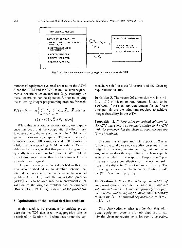
number of equipment systems) are used in the ATM. Since the ATM and the TDP share the same require- mcnts constraint characteristics (e.g, Property 1), these constraints can be tightened further by solving the following integer programming problem for each:

PrA(t) :~" = min { teri=,E ~ ~r~nE Ci.,~.,Y,,~ : .~satisfies

(9) - (12) , .,Y> 0, integer}.

While this necessitates solving an IP, our experience has been that the computational effort is not intensive due to the ease with which the ATM can be solved. For example, a typical TDP in our test cases involves about 300 variables and 160 constraints while the corresponding ATM consists of 30 variables and 25 rows, so that this preprocessing routine typically takes less than two minutes. We limit the use of this procedure so that if a two-minute limit is exceedcd, we forgo it.

The prcprocessing methods described in this scc- tion were embedded in an iterative scheme that alternately passes information between the original problem (the TDP) and the aggregated problem (ATM), and can be used until no improvement in the solution o f the original problem can be observed (Rogers et al., 1991). Fig. 2 describes thc procedure.

5. Optimization of the tactical decision problem

In this section, we present an optimizing procedure for the TDP that uses the aggregation scheme described in Section 4. Before describing the ap-

proach, we define a useful property of the clean up requirements vector.

Definition 3. The vector (of dimension r × 1 ; r = 1, 2 . . . . . ]TI) of clean up requirements is said to be r-minimal if the clean up requirements for the first r time periods are the minimum required to achieve integer feasibility in the ATM.

Proposition 2. I f there exists an optimal solution for the ATM, there exists an optimal solution to the ATM with the property that the clean up requirements are ( T - 1) minimal.

The intuitivc interpretation of Proposition 2 is as follows: the total clean up capability on scene at time point t can exceed requirement %, but not by an amount more than the capability of the least capable system included in the response. Proposition 2 permits us to focus our attention on the optimal solutions that satisfy the ( T - 1) minimal property. The following observation characterizes solutions with the ( T - 1) minimal property.

Observation I. Since the clean up capabilities o f equipment systems degrade over time, in an optimal solution with the ('1"- 1) minimal property, no equipment system will be deployed earlier than necessary to meet the ( T - 1) minimal requirements, % (t = 1,

.... I T I - 1).

This observation emphasizes the fact that additional equipment systems are only deployed to satisfy the clean up requirements for each time period

A.V. Srinivasa, W.E. Wilhelm~European Journal of Operational Research 102 (1997) 554-574 565

Table 2 Galveston Bay Area: Characteristics

Number of Component Types Number of Equipment System Types Number of Response Systems Number of Storage Locations Number of Critical Time Points Number of Potential Staging Areas

Table 3 Galveston Bay Area: Response Requirements

: 30 Critical Time Point Response Requirement (Gallons/hour)

: 9 1 8000 : 90 2 15000 : 6 3 25 000 : 5 4 35000 : 2 5 45 000

because no benefit is obtained by deploying an equipment system that is only necessary to meet minimal clean up requirements, %, of a later time period.

We now state a proposition that characterizes the nature of ( T - 1 ) minimal solutions and is used to generate facets for the requirements subpolytope of the TDP (associated with inequality (2)).

Hous~ S~I~ a~

I.~ft Bay

Baytown

Galveston Bay

N

s~,~ng ~ 2 J ~ . San Leon'

Texas CS.ty . O , Entrance

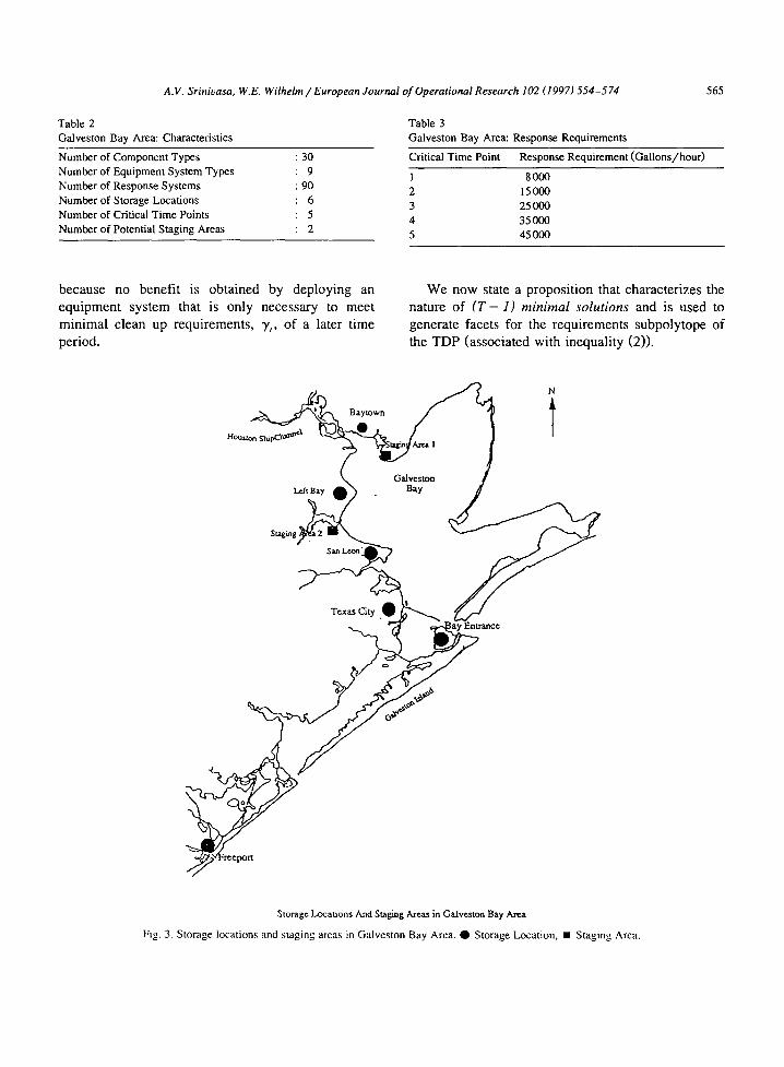
Storage Locations And Staging Areas in Galveston Bay Area

Fig. 3. Storage locations and staging areas in Galveston Bay Area. • Storage Location, • Staging Area.

566 A. V. Srinivasa, W.E. Wilhelm / European Journal of Operational Research 102 (1997) .5.54-- 574

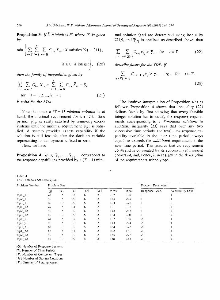
Proposition 3. If X minimizes P' where P' is gil)en by

m i n i E ~ E Ci,.,Xi~:Xsatisfies(9) - ( 1 1 ), tET i=l ~rG[l

X > 0, X integer) , (20) /

then the family of inequalities given by

± ' i=1 ~r~11 i=1 ~ E / /

for t = 1,2 ..... [TI-- 1 (21)

is valid for the ATM.

Note that once a ( T - 1) minimal solution is at hand, the minimal requirement for the ]T[th time period, ~':rl, is easily satisfied by removing excess systems until the minimal requirement ~'p.. is satisfied. A system provides excess capability if the solution is still feasible after the decision variable representing its deployment is fixed at zero.

Thus, we have

Proposition 4. I f y~, T2 . . . . . Y ; r i - ~ correspond to the response capabilities provided by a ( T - 1) mini-

mal solution (and are determined using inequality (21)), and 7'rl is obtained as described above, then

~ C,,,,Xiq > ~,, for t ~ T (22) i=1 q~O(t)

describe facets for the TDP, if

E Ct, t: i,qUq > 'Yt+l - "Yt, for q~R(t+ I)

t ~ T .

(23)

The intuitive interpretation of Proposition 4 is as follows: Proposition 4 shows that inequality (22) defines facets by first showing that every feasible integer solution has to satisfy the response require- merits corresponding to a T-minimal solution. In addition, inequality (23) says that over any two successive time periods, the total new response capability available in the later time period always equals or exceeds the additional requirement in the new time period. This assures that no requirement constraint is dominated by its successor requirement constraint, and, hence, is necessary in the description of the requirements subpolytope.

Table 4 Test Problems Set Description

Problem Number Problem Size

IQI ]Ti IEI IMI [Xl # r o w t d p l _ l l 42 5 31 6 2 107 t d p 2 _ l l 90 5 30 6 2 143 t d p 3 _ l l 60 10 30 5 2 164 t dp l_12 42 5 31 6 2 101 tdp2_12 90 5 30 6 2 143 tdp3_12 60 10 30 5 2 164 tdpl_21 42 5 31 6 2 107

tdp2_..21 90 5 30 6 2 143 tdp3_21 60 10 30 5 2 164 tdp l_22 42 5 31 6 2 102 tdp2_22 90 5 30 6 2 135 tdp3_22 60 10 30 5 2 158

Problem Parameters

#co l Response Level Availabil i ty Level 138 1 1 294 1 1 372 1 I 132 1 2 283 I 2 36O I 2 138 2 1 294 2 I 372 2 1 13I 2 2 277 2 2 353 2 2

]QI: Number of Response Systems [7"[: Number of Time Periods I El: Number of Component Types !M]: Number of Storage Locations iKi: Number of Staging Areas.

A.V. Srinivasa, W.E. Wilhelm / European Journal of Operational Research 102 (1997) 554-574 567

6. Computational evaluation

This section describes the test problems used to evaluate the solution method. It also discusses test results.

6.1. Test problems

Our numerical test problems are based on an actual setting in the Galveston Bay Area. We defined three "base" cases and four variations of each, representing the combinations of two levels of each of two factors. To illustrate the base cases, we describe one in some detail.

For the second base case, we identified nine types of equipment systems that we used to generate a

total of 90 response systems by considering the locations at which the constituent components are stored and the staging area where each response system is composed. The planning horizon consists five critical time points (i.e., five time periods). Table 2 itemizes some characteristics of the Galve- ston Bay Area relative to the second base case. Response requirements are specified in Table 3. Fig. 3 depicts the Galveston Bay Area, including the six locations that store components and the two areas that might be used for staging.

We now describe the 12 test problems used to evaluate our two heuristics. Three factors were con- sidered in defining each test problem: size (determined by the number of critical time points and number of response systems used), response require-

Table 5 Bounds on Equipment Systems (ES)

ES # P r o b # 1_11 2_11 3__11 1_12 2 _ 1 2 3_12 1_21 2_21 3_21 1 2 2 2 2 2 3_22

ESiL: 7 15 11 7 16 11 7 15 11 7 15 1 ]

1 ES.rt" 1 10 4 1 9 4 0 10 4 1 11 6 ESTu 1 11 5 I 12 6 1 10 5 1 11 6

ESIv 7 2 13 7 6 13 7 2 13 7 2 13

2 ES tL 0 2 4 0 2 5 0 2 5 0 2 7

ES.rL: 0 2 7 0 4 8 0 2 7 0 2 7 ESlu 4 2 5 4 2 5 4 2 5 4 2 5

3 ES .-r. L 0 0 0 0 0 0 0 0 0 0 0 0

ES-rc 0 0 2 0 2 1 0 0 1 0 0 3 ESIc. 9 6 8 9 2 8 9 6 8 9 6 8

4 ES.rt. I 0 1 1 0 1 0 0 2 1 0 2 ES.r-: 1 1 2 1 2 2 t 0 2 1 0 3

ES t,,; 21 3 4 21 2 4 21 3 4 21 3 4

5 [z'S TL 1 0 4 1 0 4 0 0 4 0 0 0

ESTt: 1 0 4 1 2 4 1 0 4 0 0 0 ES Iu 8 3 20 8 5 20 8 3 20 8 3 20

6 ES.rl. 0 3 1 0 3 2 0 3 2 0 3 4 ES n : 0 3 6 0 3 5 0 3 5 0 3 7

ESit: 5 4 15 5 4 15 5 4 15 5 4 15

7 ESTt 3 4 0 4 4 0 3 4 1 4 4 6 ES ru 3 4 5 4 4 3 3 4 4 4 4 7

ESlu 7 18 13 7 18 13 7 18 13 7 18 13

g ES.rt 0 1 0 0 0 0 0 1 0 0 3 0 ESTc 0 1 0 0 2 0 0 1 0 0 3 0

ES ~u 5 20 9 5 20 9 5 20 9 5 20 9

9 ESv t 2 11 0 0 0 0 2 12 0 0 2 0

ES.rts 2 12 0 0 1 0 2 13 0 0 2 0 ESIu 16 - 16 - - 16 -- 16

10 ESTI - - 0 0 - - 0 - 0

g s I't: 0 - 0 -- 0 -- 0

ES~u: Initial Upper bound: ESH.: Tightened Lower bound; ESrv: Tightened Upper bound.

568 A.V. Srinivasa, W.E. Wilhelm/European Journal o f Operational Research 102 (1997) 554-574

Table 6 Bounds on the total number of response systems, and number of variables fixed

Problem # Nt. N o, Number of variables fixed

tdpl_l I 8 8 7 tdp2 l 1 32 32 21 tdp3_l 1 22 23 80 tdpl_12 7 7 7 tdp2_12 20 22 17 tdp3_12 21 25 74 tdpl_21 7 7 5 tdp2_21 32 33 18 tdp3_21 22 23 76 tdpl 2 2 6 6 5 tdp2_22 25 27 14 tdp3_22 29 30 69

ments (y,, t ~ T) and component availability (A~,,,). Consequently, problems of three different sizes composed the "base" cases and other problems were created from each base case by taking different combinations of the response requirement and component availability. Thus, each test problem was created from a "base" case by fixing each of two factors at one of two levels.

Table 4 describes the test problems. For example, tdp2_ll represents the second "base" case and level 1 for both the response scenario and component availability factors, tdp2 11 involves 90 response systems, five time periods, 30 components stored in

six locations, and two staging areas. Similarly, tdp3 12 represents the third "base" case with response requirement and component availability at levels 1 and 2, respectively. Each of the test problems is based on the Galveston Bay Area and thus portrays characteristics that are expected to reflect an actual spill.

6.2. Test results"

Our solution approach, which combines thc cut generation method with a branch and bound algorithm, starts by developing the aggregated model for the problem and then uses the ATM and thc TDP in the itcrative scheme for preprocessing described in Section 4. After preprocessing, the inequalities described by (16) are generated. If the preprocessing procedures and the facets for the requirements constraints do not yield an integer solution, we resort to branch and bound for the TDP. The branch and bound algorithm exploits the "lower triangular" structure (Section 4) to define special branching rules. The preprocessing and cut generation routines are coded in FORTRAN, and we employ the IBM OSL branch and bound solver.

Tables 5-8 summarize the results. Table 5 shows the Dower aud upper bounds for equipment system types in each test problem obtained by tightening the GLB and GUB constraints using Eqs. (14) and (15),

Table 7 Computational Evaluation

Prob# LP Relaxation LP Relaxation IP Optimal Run time Reduction before reformulation after reformulation Solution (seconds) in Gap, (%)

tdp I _ 11 154.02 185.00 185.00 5.55 100.00 tdp2 l 1 788.84 901.00 910.00 733.80 92.57 tdp3__ l 1 758.40 780.68 805.00 2 526.10 47.8 I tdp I 12 134.79 143.50 150.00 4.63 57.26 tdp2.12 378.74 381.00 391.00 4 075.00 18.43 tdp3 12 719.45 732.41 741.00 6190.24 60. la tdp I _21 145.01 173.00 173.00 4.52 100.00 tdp2 21 797.25 908.27 9!0.00 911.40 98.47 tdp3__21 762.13 789.45 805.00 1 221.14 63.73 tdpl 2 2 124.90 131.50 138.00 8.47 50.38 tdp2 22 468.49 538.73 575.00 2 334.00 65.95 tdp3_ 22 890.67 951.77 959.00 3 814.42 89.42

(1) All times are in seconds. (2) All runs were carried out on IBM RISC System/6000, Model 550 machine.

A.V. Srini~asa, W.E. Wilhelm/European Journal of Operational Research 102 (1997) 554-574 569

Table 8 Comparison of the four procedures

Prob# Heuristic I Heuristic II LP Relaxation Aggregation-SCP Procedure

Solution Run Solution Run Solution Run Solution Run Value Time Value Time Value Time Value Time

Best OSL B and B Solution After 300 Seconds

tdpl_l 1 185.00 0.14 187.00 0 . 4 1 154.02 0.05 185.00 5.55 tdp2_l 1 913.00 1.66 945.00 13.40 788.84 0.80 910.00 733.80 tdp3 11 806.00 1.28 805.00 10.11 758.40 0.14 805.00 2526.10 tdpl_12 150.00 0.12 150.00 2.00 134.79 0.04 150.00 4.63 tdp2_12 456.00 0.69 448.00 8.53 378.74 0.16 391.00 4075.20 tdp3_12 753.00 1.56 784.00 25.23 719.45 0.15 741.00 " 6 190.24 tdpl_21 173.00 0.12 173.00 0.73 145.01 0.07 173.00 4.52 tdp2 21 992.00 1.07 1 039.00 10.01 797.25 0.11 910.00 911.40 tdp3_21 828.00 2.51 805.00 10.18 762.13 0.15 805.00 1 221.14 tdpl_22 138.00 0.12 138.00 0.50 124.90 0.03 138.00 8.47 tdp2_22 580.00 0.57 580.00 1.10 468.49 0.17 575.00 2334.00 tdp3_22 989.00 3.36 983.00 8.55 890.67 0.39 959.00 3 814.42

1 8 5 . 0 0 "

150.00 ° 698.00 784.00 t73.00 '

889.00 138.00 " 629.00 983.00

(1) All times are in seconds. (2) All runs were carried out on an IBM RISC System/6000, Model 550 machine.

respectively. For comparison, we also show the initial upper bounds on the equipment system types. The initial lower bound for all equipment systems is zero in all the test problems and hence is not shown in Table 5. Bounds for equipment system 10 are not shown for base cases 1 and 2, since these do not include equipment system 10. The bound tightening procedures are effective, closing initial ranges of about 10 to an average of 2.

Table 6 shows the effectiveness of preprocessing routine (described by Eqs. (16) and (17)) with respect to the bounds on the total number of equipment systems necessary [NL, Nt/] and in terms of the number of variables fixed by reduced cost fixing and Proposition 1. Table 7 compares the value of the LP relaxation to that of the original TDP, the value of the LP relaxation after the cuts are added, and the IP optimal solution. The run times (in seconds) for obtaining IP optimal solutions are also shown. Table 8 compares the pertormance of this optimizing approach with that of the two heuristics developed by Wilhelm and Srinivasa and with the OSL branch and bound solver applied directly to each problem. The run times in Table 8 are all in seconds.

Results show that the aggregation scheme is suc- cessful, not only in improving bounds from the LP relaxation, but also in finding optimal integral solutions within reasonable times. The rcl"ormulation pro-

cedures coupled with the facets for the requirement constraints (described by inequality (22)) succeed in reducing the integrality gap. Indeed, for some of the smaller test problems, the method fully closes the integrality gap.

In general, for a base case, the average gap reductions were better for test problems with component availability (factor 2) at level 1, rather than level 2. However, such a relationship was not observed relative to the response scenarios (clean up requirements levels (factor 2). This suggests that the facets for the requirement constraints play a key role in reducing the gap, but to achieve larger gap reductions they have to be used in conjunction with the reformulation procedures that tighten the component availability constraints.

7. Summary and conclusions

In this paper, we formulate the TDP as a general integer program and present an optimizing approach that is based on a combination of aggregation techniques and strong cutting plane methods. The aggregation-based iterative procedure exploits special structures in the aggregated model so that we are able to tighten not only the requirement constraints, but also the component availability, the GUB, and

570 A.V. Srinivasa, W.E. Wilhelrn /EuropeanJournal of Operational Research 102 (1997) 554-574

the GLB types of constraints. We identify a family of facets for the response requirement subpolytope, derive other inequalities based on dominance properties, and compute bounds on the number of equipment systems necessary. Test results demonstrate that this approach yields an effective way to obtain optimal solutions to the TDP.

This solution approach is intended for use by managers as a decision support aid in prescribing optimal, timephased response to an oil spill. No quantitative methods are currently used to assist managers in making these important decisions. Man- agers can use the model to evaluate the combination of ways in which response can be mobilized, assur- ing optimal composition and deployment of response systems. This approach combines components, which are, perhaps, stored at diverse locations, to achieve an effective response, meeting timephased requirements, which are intended to minimize environmental impact. The model provides a structure for coor- dinating the response efforts of contractors, responsible parties, Coast Guard, state government, and othcr officials.

Managers can also use the model as a planning tool to evaluate the policies by which clean up is conducted. For example, as demonstrated by the test problems, the model could be used in (strategic) contingency planning to establish required response scenarios {y,: t ~ T}. In addition, test problems demonstrate application to evaluate systemwide response capability as a function of equipment availability and could be used, for example, to assess the need for a policy that would require contractors to provide minimum levels of equipment availability to assure adequate response capability.

The tactical decision model could easily be integrated with models that address the strategic and operational levels of response. For example, managers could use it to evaluate contingency plans, assessing the ability of the system prescribed by models that address the strategic level to respond to certain types of spills at selected risk points. The operational level typically employs a trajectory model to predict the movement and spread of oil over time. Managers could use trajectory model predictions as inputs to the tactical decision model, which could bc rerun periodically to revise prescribed response in light of changing conditions. In yet another applica-

tion, managers could employ the tactical decision model in training programs to provide decision support for trainees in prescribing response to simulated spills.

Acknowledgements

This material is based on work supported by the Texas Advanced Technology Program under Grant Number 999903-282. We are indebted to a number of individuals and organizations who have helped us assure the relevancy of this research. In particular, we acknowledge Commander John Salvesen, Po~l Operations Chief, and Lieutenant C. David Weimer, both of the U.S. Coast Guard Marine Safety Office in Galveston, Texas, for their interest in this work and for making it possible to gather data describing an application in the Galveston Bay Area. We would also like to express our appreciation to Mr. Tim McKenna, Director of the Oil Spill Prevention and Response Program, and Mr. Ronald Brinkley, Re- gional Manager of Oil Spill Prevention and Re- sponse, who are both with the Texas General Land Office. In addition, this research benefitted from discussions with a number of individuals, including Mr. Theo Camlin, Program Coordinator: Texas A& M Oil Spill Program at Galveston, Dr. Bela M. James, Environmental Specialist: Shell Oil Com- pany, and Mr. Raymond G. Meyer, Operations Man- ager: Clean Channel Association. Foremost, however, has been the advice and experience offered by Dr. RichardA. Geyer of the Offshore Technology Research Program at Texas A&M University. We acknowledge the able efforts of Dr. Sangho Joo, who helped to gather and formulate the data used in our test problems. Finally, we acknowledge two anony- mous referees whose comments allowed us to strengthen an earlier version of this paper.

Appendix A. Proofs

Proof of Property 1. If x ~ S~, from Definition 1 and by Eq. (8), it follows that X = c/~(x) satisfies inequality (9). Hence, X ~ S~.

To show that we can construct a solution x that is

A.V. Srinivasa, W.E. Wilhelm~European Journal of Operational Research 102 (1997)554-574 571

feasible relative to inequality (2), given a solution ,~" that is feasible relative to inequality (9), define

Xiq' ~ XiTr

for "all 7r ~ / 7 , and for some q' ~ Q(w) and,

Xiq ~ 0

for all other q ~ Q(w) - {q'}. Then, by Eq. (8),

i=t i=t

Z E "rrEIl(t) i=t~ qeg(t) i=%

for all t ~ 7'. Hence, X ~ S~. []

Proof of Proper ty 2. The proof is obvious, since each of the constraints in inequality (10) is obtained by taking a nonnegative linear combination of a subset of constraints in inequality (3). D

Proof of Proper ty 3. Again, the proof is straightforward, since each of the constraints in inequality (11) is obtained by taking a nonnegative linear combination of a subset of constraints in inequality (4). []

Proof of Property 4. Follows from Property 2 and Definition 2. []

P r o o f of Proposi t ion 1. Since both q~ and q2 represent the same equipment system type, the clean up capabilities of the two response systems are the same (i.e., C(~,q), = Co,q), for all t and i). Further- more, the number of components of type e required by both response systems is the same. Hence, the allocation of components between these two response systems is resolved solely according to response times. C

Proof of Proposition 2. We will prove this by showing that if X ' is any optimal solution to the ATM with Z* = r X " without the ( T - 1) minimal property, then we can derive an X, such that r X = Z*, and X has the ( i t ' - ]) minimal property.

Since (by assumption) X ' does not exhibit the (7"- 1) minimal property, there exists a t (t _< I T i - 1) such that i=t

E E Citw X i ; - ~/t i = 1 7r ~ / ' /

> min {min{C,,~., C2,_ . . . . . C,,,.~}} ( 1 9 ) {t~: x,,>0} ' "

where ~, is the response requirement for t e~ T.

Let w' (w' E El(t)) be an equipment system for which inequality (19) is satisfied in period t. Then, by postponing the use of w' in the response until time period (t + 1), the objective function remains unchanged, while feasibility is maintained. Repeat- ing the procedure for all w' (w' E / 7 ( t ) ) that satisfy inequality (19), the optimal solution now exhibits the t-minimal property. By repeating the same procedure for each of the periods t + 1, t + 2 . . . . . I T I - 1, we can achieve a solution that has the ( T - 1) minimal property. []

Proof of Proposition 3. First note that the optimum objective function value for Eq. (20) represents the minimum total clean up capability necessary to be feasible. And, by Observation 1, no equipment systems are deployed earlier than necessary. So, Yj, Y2 . . . . ,5'(7--~) represent the minimum clean up requirements in each time period to achieve feasibility. In other words, X represents the (T - 1) minimal solution for the ATM. []

Proof of Proposition 4. Proving the validity of inequalities (22) is straightforward and follows directly from Proposition 3 and Property 2.

To show that inequalities (22) describe facets, note that by definition of ~,,(t ~ T) , there does not exist an 2~( 2 ~ PI D) such that

E Ciq xi u < ~/t, for t E T. i = I q~Q(t)

F u r t h e r m o r e , the c o n d i t i o n T, > Y,+~ - ~q ~ n(,+ i)C,-r i,q assures that each requirement constraint is necessary in the description of ltD. The result follows. []

Appendix B. A numerical example

Notation

H Q

T J Q( j)

set of equipment system types = {Try, 7r2} set of response system types = {q~, q2, q3,

q4} set of time periods = { 1, 2, 3} set of staging areas = {a, b} set of response systems that can be staged in staging area j

572

Q('n')

M

A.V. Srinivasa, W.E. Wilhelm / European Journal o f Operational Research 102 (1997) 554 - 5 7 4

set of response systems that employ equip- E set of equipment component types = {el, e2} merit system type 7/" Xtq number of response systems of type q de- set of storage locations = {mj, m 2} ployed in time period t.

Description of Response Systems

Response Equipment (Component- Quantity Time Staging Response System System Location) required available Area Time

qj 7r I e lm k 3 1 a 10 q2 7rl e lm 2 3 2 b 18 q3 7r2 e lmj 4 1 a 12

e2m 2 5 q4 ~2 ej m 2 4 3 b 25

e~m~ 5

Description of Equipment Systems

Equipment Clean up capability Required Response

System Barrels/day Periods After Deployment Staging Area Time

7rj 500 0 250

450 I 405 2

zr 2 900 0 800 1 650 2

10

400 12

The Tactical Decision Problem (nonnegativity and integer restrictions are omitted for brevity)

Minimize Response Time =

10 x u + 10 x21 + l0 x31 + lg x22 + 18 x32 + 12 xr3 + 12 x23 + 12 x33 Timestaged Response Requirements 500 xl~ +900 x~:

450 x~ +500 x2~ +500 x22 +800 xj3 +900 x23

405 xll +450 x21 +500 131 +450 x22 +500 x32 +650 xt3 +800 x23 +900 x33 Component Availability at Storage Locations

3 X~I +3 X21 +3 X31 + 4 X13 +4 X23 + 4 X33 3 x22 + 3 x3_,

Staging Area Constraints 250 xtl

+250 x2~

5 x13

+ 400 x 13

+ 5 x23 + 5 x33

+ 400 x23 +250 x3s +400 x3~

+250 x,~.

GUB Constraints

Xll +1"21 +.1"31

+AII +.1"23 +X33

+ 250 x3z

+ff22 +X32

+28 x3a

+ 900 x 34

+ 4 x34

5 x34

+ 400 x34

X34

> 3600 >_ 7500 ;> 12000

< 34 < 1 8 ~ 1 5 _< 40

< 3000

< 3000 < 3000 _<2500 _< 2 500

< 7 _<4

< 6 _<3

A.V. Srinivasa, W.E. Wilhelm / European Journal of Operational Research 102 (1997) 554-574

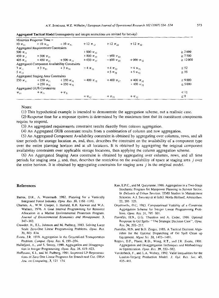
Aggregated Tactical Model (nonnegativity and integer restrictions are omitted for brevity)

573

Minimize Response Time = 10 -n-ll + 10 "n'2L + 10 "rr3] + 12 rq2 + 12 'rr22 + 12 "n-32 Aggregated Requirements Constraints 500 "n-ll +900 7rl, - 450 7rLi +500 7r21 + 800 "trl2 +900 ~2-, 405 ~'l~ +450 ~'21 +500 "rr3~ +650 7r~2 +800 7r22 +900 rr32 Aggregated Component Availability Constraints 3 7r~ + 3 q'r21 + 3 71"31 -I-, 4 "n-j2 +4 "n'22 + 4 "tr32 5 ~r12 +5 "n'22 +5 w32 Aggregated Staging Area Constraints 250 "rrl] +250 -n'21 +250 'rr31 +400 -rr12 +400 7r22 +400 7r32

+ 250 7r2t +250 ~'31 + 400 "n-32 Aggregated GUB Constraints "rrlu + "n'21 +~r31 < I1

+ 7rl2 + 71"22 + "rr32 ~; 9

k 3600 > 7 500 > 12000

_< 52 < 55

< 9000 < 5000

Notes :

(1) T h i s hypo the t i c a l e x a m p l e is i n t ended to d e m o n s t r a t e the agg rega t ion scheme , no t a real is t ic case.

(2) R e s p o n s e t ime for a r e s p o n s e sys t em is d e t e r m i n e d by the m a x i m u m t ime that its cons t i t uen t c o m p o n e n t s

r equ i re to respond .

(3) A n a g g r e g a t e d r e q u i r e m e n t s cons t r a in t resul t s d i rec t ly f rom c o l u m n aggrega t ion .

(4) A n A g g r e g a t e d G U B cons t r a in t resu l t s f rom a c o m b i n a t i o n o f c o l u m n and row aggrega t ion .

(5) A n A g g r e g a t e d C o m p o n e n t Ava i l ab i l i t y cons t r a in t is ob t a ined by agg rega t ing ove r c o l u m n s , rows, and all

t ime pe r iods for s to rage loca t ion m, and, thus, desc r ibes the cons t r a in t on the ava i lab i l i ty o f a c o m p o n e n t type

ove r the en t i re p l a n n i n g h o r i z o n and at all loca t ions . It is ob t a ined by agg rega t ing the or ig ina l c o m p o n e n t

ava i l ab i l i ty cons t r a in t s o v e r app l i cab le s torage loca t ions , then app ly ing the c o l u m n agg rega t ion s cheme .

(6) A n A g g r e g a t e d S tag ing Area cons t r a in t is ob t a ined by agg rega t i ng ove r co lumns , rows, and all t ime

per iods for s t ag ing a rea j , and, thus, desc r ibes the res t r ic t ion on the ava i lab i l i ty of space at s t ag ing area j o v e r

the en t i re hor izon . It is ob t a ined by agg r ega t i ng cons t r a in t s for s t ag ing area j in the or ig ina l mode l .

R e f e r e n c e s

Barros, D.R., A. Weintraub. 1982. Planning for a Vertically Integrated Forest Industry. Opns. Res. 30, 1168-1182.

Charnes, A., W.W. Cooper, J. Harrald, K.R. Karwan and W.A. Wallace, 1976. A Goal Interval Programming for Resource Allocation in a Marine Environmental Protection Program. Journal of Environmental Economics and Management. 3, 347-362.

Crowder, H., E.L. Johnson and M. Padberg, 1983. Solving Large Scale Zero-One Linear Programming Problems. Opns. Res. 31, 803-834.

Evans, J.R. 1979. Aggregation in the Generalized Transportation Problem. Compur Opns'. Res. 6, 199-204.

Hallefjord, A., and S. Storoy, 1990. Aggregation and Disaggrega- tion in Integer Programming. Opns. Res. 38, 619-623.

Hoffmann, K.L. and M. Padberg, 1991. Improved LP-Representa- tions of Zero-One Linear Programs for Branch-and-Cut. ORSA Jou. on Computing, 3, 121-134.

Kao, E.P.C., and M. Queyranne. 1986. Aggregation in a Two-Stage Stochastic Program for Manpower Planning in Service Sector. In Delivery of Urban Services. TIMS Studies in Management Sciences. A.J. Swersey et al (eds). North-Holland, Amsterdam. 22, 205-225.

Onyekwelu, D.C. 1983. Computational Viability of a Constraint Aggregation Scheme for Integer Linear Programming Prob- lems. Opns. Res. 31,795-801.

Psaraftis, It.N., G.G. Tharakan and A. Ceder, 1986. Optimal Response to Oil Spills: "The Strategic Decision Case", Opra'. Res. 34, 203-217.

Psaraftis, H.N. and B.O. Ziogas, 1985. A Tactical Decision Algo- rithm for the Optimal Dispatching of Oil Spill Clean up Equipment. Mgmt Sci. 31, 1475-1491.

Rogcrs, D.F., Plante, R.D., Wong, R.T., and J.R. Evans, 1991. Aggregation and Disaggregation Techniques and Methodology in Optimization. Opns. Res. 39, 553-582.

Vanderbeck, F., and L.A. Wolsey, 1992. Valid Inequalities for the LasdonrTerjung Production Model. J. Opl. Res. Sac. 43, 435--441.

574 A. V. Srinivasa, W.E. Wilhelm/European Journal of Operational Re,search 102 (1997) 554-574

Wemmerlov, U., and N.L. llyer. 1986. Procedures for Part Fam- i ly/Machine Group Identification Problem in Cellular Manu- facturing. J. Opns. Mgmt. 6, 125-147.

Wilhelm, W.E., and A.V. Srinivasa. forthcoming. Tactical Re- sponse in Oil Spill Clean Up Operations. Management Sci- ence.

Zipkin, P.II., 1980a. Bounds for Aggregating Nodes in Network Problems. Math. Prog. 19, 155-177.

Zipkin, P.H., 1980b. Bounds on the effect of Aggregating Vari- ables in Linear Programs. Opns. Res. 28, 403-418.

Zipkin, P.11., 1980c. Bounds for Row Aggregation in Linear Programming. Opns. Res. 28, 9(13-916.

Documents

EUROPEAN JOURNAL RESEARCH ELSEVIER Theory … strategic/elsvier/el537.pdf · Theory and Methodology A procedure for optimizing tactical response in oil spill clean up ... tactical