Embed Size (px)
Citation preview
European Journal of Operational Research 263 (2017) 961–973
Contents lists available at ScienceDirect
European Journal of Operational Research
journal homepage: www.elsevier.com/locate/ejor
Decision Support
Goal congruence analysis in multi-Division Organizations with shared
resources based on data envelopment analysis
Jingjing Ding
a , Wei Dong
b , Liang Liang
a , Joe Zhu
c , ∗
a School of Management, Hefei University of Technology, No. 193 Tunxi Road, Hefei, Anhui Province 230 0 09, PR China b School of Management, University of Science and Technology of China and USTC-CityU Joint Advanced Research Centre, 166 Ren’ai Road, Suzhou, Jiangsu
Province 215123, PR China, c Foisie School of Business, Worcester Polytechnic Institute, 100 Institute Road, Worcester, MA 01609, USA
a r t i c l e i n f o
Article history:
Received 15 December 2016
Accepted 15 June 2017
Available online 20 June 2017
Keywords:
Data envelopment analysis (DEA)
Goal congruence
Nonparametric
Shared resource allocation
Optimizable operation
a b s t r a c t
In multi-division organizations, goal congruence between different divisions and top management is criti-
cal to the success of management. In this paper, drawing upon a nonparametric framework to model pro-
duction technology, we derive a necessary and sufficient condition for a firm with multiple divisions to
be goal-congruent, and then extend it to a goal congruence testing measure, which coincides with a data
envelopment analysis (DEA) model. The goal congruence measure not only shows empirically whether
the firm is goal-congruent or not, but also provides a measurement for the degree of goal incongruence.
To be goal-congruent, resources shared among divisions are suggested to be allocated so that the condi-
tions for an optimizable operation are satisfied. In addition, goal-congruent firms are verified to be cost
efficient. All findings in this research are examined and illustrated with a dataset of 20 bank branches
with shared resources for service and sales divisions.
© 2017 Elsevier B.V. All rights reserved.
1
c
(
c
(
n
w
w
d
a
a
m
v
r
b
E
fi
t
D
o
p
i
o
a
v
a
t
B
F
1
V
a
c
d
s
r
(
2
h
0
. Introduction
In management accounting, goal congruence is defined as the
onsistency or agreement of individual goals with company goals
Atkinson, Kaplan, Matsumura, & Young, 2012 ; Itami, 1975 ). Goal
ongruence is deemed as the intent of organizational control
Flamholtz, Das, & Tsui, 1985 ; Malmi & Brown, 2008 ). The orga-
ization will realize its goal more effectively and perform better
hen goals of multiple production divisions can be well aligned
ith organizational plans. However, scholars have argued that in-
ividual and organizational goals are inevitably at odds with one
nother ( Witt, 1998; Yamoah, 2014 ). In this paper, we investigate
testing technique to answer empirically whether the goals of top
anagement (i.e., the organization as a whole) and individual di-
isions are congruent in an organization environment with shared
esources, and to what extent they are divergent. This paper is
uilt upon the notion of profit function and offers the popular Data
nvelopment Analysis (DEA) technique new insight that can bene-
t the studies in both the management accounting and organiza-
ion theory.
∗ Corresponding author.
E-mail addresses: [email protected] (J. Ding), [email protected] (W.
ong), [email protected] (L. Liang), [email protected] (J. Zhu).
o
t
t
w
ttp://dx.doi.org/10.1016/j.ejor.2017.06.040
377-2217/© 2017 Elsevier B.V. All rights reserved.
As a key issue in determining the fit between individuals and
rganizations, goal congruence has long been one of the central
roblems in the organization theory ( Kristof, 1996; Vancouver, Mil-
sap, & Peters, 1994 ). Under the setting of a large firm that consists
f one central office and many functional divisions, management
ccounting literature has recognized the important role that the di-
ergence of interests between top management and division man-
gers and the private information of division managers concerning
heir work play in the budgeting process ( Baiman & Rajan, 2002 ;
rown, Fisher, Sooy, & Sprinkle, 2014 ; Douthit and Stevens, 2015 ;
isher, Maines, Peffer, & Sprinkle, 2002; Harris, Kriebel, & Raviv,
982; Heinle, Ross, & Saouma, 2014 ; Rajan & Reichelstein, 2004 ;
an der Stede, 2011 ). In particular, when resources are shared
mong functional divisions in large firms, budgeting becomes more
omplicated, because it is hard to evaluate a division’s operation
ue to the fact that consumed shared resources cannot be ob-
erved. Studying the issues related to allocate the cost of shared
esources will help budgeting systems function better in practice
Cook, Hababou, & Tuenter, 20 0 0; Ding, Feng, Bi, Liang, & Khan,
014 ).
Schaffer (2007) identifies four types of goal congruence in
rganizations, namely, constructive goal congruence, construc-
ive goal incongruence, destructive goal congruence, and destruc-
ive goal incongruence. “Constructive” and “destructive” indicate
hether goals are clearly communicated (i.e., constructive) or not
962 J. Ding et al. / European Journal of Operational Research 263 (2017) 961–973
t
s
d
m
t
i
f
i
o
o
a
p
i
s
s
i
T
m
d
w
o
N
t
s
r
t
m
o
g
i
l
t
t
t
s
v
H
n
s
o
D
m
m
i
t
a
t
a
g
F
p
d
fi
m
r
b
g
s
n
n
a
t
o
(i.e., destructive). “Congruence” and “incongruence” mean whether
front-line employees buy the top management’ goals (i.e., congru-
ence) or not (i.e., incongruence). Two examples are shown here
to offer a better understanding of “destructive” and “construc-
tive” goal incongruence respectively. In one example, taken from
Schaffer (2007) , the top management of a company sets up a new
goal for improving product quality, but the division management
are still enjoying the initial success in reducing operating costs.
Additionally, they may think achieving the new goal would incur
additional costs. Without a clear emphasis on the goal changing
when communicating to front-end employees, employees may still
work for the initial goal. Messages can be misunderstood as a re-
sult. The other example is taken from Fruitticher, Stroud, Laster,
and Yakhou (2005) about American United Life company. The ul-
timate goal of the company is that the internal rate of return
achieves 12%. The company, however, notices that division man-
agers are not willing to spend $250,0 0 0 for mass advertising that
would bring in $650,0 0 0 of annual premiums because it would
lead to the overrun of the division’s operating budget. If division
managers would have bought the goal and spent the money, the
organization’s goal could be accomplished easily.
The role of goal congruence is nontrivial. For the top manage-
ment, the designs or strategies developed, without the agreement
and compliance of low-level members, are often deferred and re-
jected ( McKelvey & Kilmann, 1975 ). Yamoah (2014) suggests that
goal congruence is very important to attain organization’s strategic
objectives and ensure the coordination and motivation of all em-
ployees concerned. If goal incongruence is not stopped in time, it
will encourage organizational actors to pursue individual goals at
the expense of the official organizational objectives. Johnson, Pfeif-
fer, and Schneider (2013) mention that agency conflicts between
divisions affect the design of capital charge rates and asset-sharing
rules in the two-stage capital budgeting decisions for shared in-
vestments. Empirical studies show that ( 1 ) employees’ job satis-
faction, commitment, and intentions to quit are related with goal
congruence ( Vancouver & Schmitt, 1991 ), ( 2 ) well-communication
( Meyers, Riccucci, & Lurie, 2001 ), trust and shared values ( Scott
& Gable, 1997 ), among others, can help to improve the congru-
ent level, ( 3 ) goal congruence is important to attain organization’s
strategic objectives ( Yamoah, 2014 ), and is able to augment em-
ployees’ productivity ( Zhang, Wang, & Shi, 2012 ) and enhance or-
ganizational performances ( Ayers, 2015 ), (4) goal congruence in
top management team mediates the relationship between CEO
transformational leadership and vice president’s attitude ( Colbert,
Kristof-Brown, Bradley, & Barrick, 2008 ), and (5) goal congruence
moderates the relationship between organizational politics and job
performances ( Witt, 1998 ).
If the congruence issue is to be treated formally, a measure
for the congruence between top management and divisional man-
agers is warranted. According to Edwards (1994) , most commonly
used operational measures of goal congruence are bivariate con-
gruence indices such as algebraic difference and absolute differ-
ence, and the index of profile similarity. Then, the directly mea-
sured goal congruence indices are treated as explanatory variables
for other dependent variables relevant to the employee or organi-
zation. Edwards (1994) examines problems with these congruence
indices and presents an alternative approach that overcomes these
problems. The proposed approach (i.e., response surface analysis)
is widely applied to organizational and psychological studies (e.g.,
Tafvelin, Schwarz, & Hasson (2017) and Human, Dirks, Delongis, &
Chen, 2016 ). In all the indices, goal congruence is always measured
in a qualitative way. For example, supervisors and subordinates are
invited to rate a range of goals using a 7-point Likert rating scale,
and similarity is calculated to represent the degree of congruence
( Ayers, 2015; Colbert et al., 2008 ). As subjective rating has limits,
in this study we develop a new quantitative method to measure
he level of goal congruence between top management and divi-
ion managers based on observational objective input and output
ata and let data speak for themselves. Furthermore, the proposed
easure is able to suggest the sources of the goal incongruence.
In this study, we shall start with the characterization of the op-
imizable operation of the overall firm and the individual divisions
n it that consume shared inputs. It should be noted that the dif-
erence between ‘optimizable operation’ and ‘optimum operation’
n this study is not trivial and worthy of discussion. To claim the
peration is optimal, one should at least specify the goal or goals
f the operation and the potential best level or levels of the oper-
tion. Then, the data of operation can be compared with the best
otential to determine whether the operation is optimal. However,
n some situations one might not have enough information to an-
wer whether the operation is optimal. Instead, the data might be
ufficient to determine a week version of optimality, i.e., the exist-
ng evidence is not against the claim that the operation is optimal.
he current study dubs the weak version of optimality as ‘opti-
izable operation’. We propose that the operation of a firm or a
ivision will be optimizable if it can achieve the maximum profit,
hich indicates that this study specifies profit maximization as an
perational goal to introduce the idea of testing goal congruence.
otice that profit maximization is not the end but the means of
he study . One may argue that an organization might not purse the
ingle goal of profit. This is true. In general cases, it is suitable to
eformulate the idea of the profit function as a value function and
he value of the function equals the level of utility (e.g., revenue)
inuses the level of disutility (e.g., cost). It shall be clear that the
nly requirement for the proposed method to be applicable in the
eneral cases is that the utility and disutility functions character-
ng the goals of divisional and organizational managers all have a
inear and additive structure.
Then it follows with the formal definition of goal congruence
hat the goal congruence exists when a specific firm under evalua-
ion and its divisions can meet some specific conditions to achieve
he maximum profit at the same time. It will be proven in this
tudy that an optimizable firm with goal-congruent multiple di-
isions is equivalent to being efficient by means of a DEA model.
ence, we leverage the DEA evaluation model as a testing tech-
ique for goal congruence. The efficiency will be viewed as a mea-
ure for assessing the degree of goal congruence. In addition, an
ptimal allocation scheme of shared inputs is obtained from this
EA-based evaluation model, together with a possible improve-
ent plan for goal congruence. At last, the goal congruence testing
easure is investigated to be a powerful one in terms of discrim-
nating capability compared with the cost efficiency definition in
he literature ( Cherchye, Rock, Dierynck, Roodhooft, & Sabbe, 2013 ),
nd based on more relaxed assumptions than the existing litera-
ure ( Cherchye, De Rock, & Walheer, 2016 ; Varian, 1984 ).
The current research contributes the literature by introducing
quantitative assessment method for the organizational goal con-
ruence and extending the functionality of the DEA technique.
irstly, the insight that the suggestions for a goal congruence im-
rovement in terms of resource allocation and cost sharing are en-
ogenous to DEA models is missing in the conventional application
elds of DEA models. In addition, the insight is gained through the
ethods that are based on more relaxed assumptions than similar
esearches in the DEA literature. Secondly, the proposed method is
ased on objective input and output data in evaluating goal con-
ruence, rather than subjective ratings together with difference or
imilarity measures that are the prevalent practices in the orga-
ization behavior and management accounting literature. Last but
ot the least, though based on the profit maximization as an oper-
tional behavioral objective, the proposed method is applicable if
he optimizing behaviors of decision makers are defined as other
bjectives such as utility maximization. The only requirement of
J. Ding et al. / European Journal of Operational Research 263 (2017) 961–973 963
o
o
i
b
c
g
b
c
i
v
S
2
o
t
s
i
r
l
t
(
p
s
p
v
t
m
a
a
i
u
d
i
p
c
d
s
o
t
s
C
s
d
t
a
s
a
t
fi
s
p
a
u
i
p
s
m
c
a
c
e
C
a
a
d
Z
m
(
s
a
i
i
t
a
o
a
t
t
D
p
i
g
w
w
p
i
A
i
o
e
c
“
w
s
r
m
t
s
t
b
a
t
s
b
s
p
p
w
s
m
s
t
t
b
i
b
b
n
m
s
p
o
s
ur analyses is that the measures that decision makers attempt to
ptimize can be formalized in a linear and additive structure.
The rest of the paper is organized as follows. Section 2 reviews
ssues related to shared inputs allocation for goal congruence faced
y organizations. After analyzing the optimizing behavior and goal-
ongruent behavior of firms, a DEA-based model for measuring
oal congruence is developed in Sections 3 and 4 . The difference
etween the proposed goal congruence measure and the cost effi-
iency measure in literature is compared in Section 5 . An empir-
cal testing for a set of bank branches with shared inputs is pro-
ided in Section 6 . Conclusions and discussions are presented in
ection 7 .
. Literature review
In this paper, the goal congruence issue is investigated in an
rganization environment with shared resources. Since the litera-
ure about goal congruence has been introduced in the preceding
ection to motivate the current work, this section is dedicated to
ntroduce the literature about shared resources allocation and the
esearch technique in an effort to clarify our contribution to this
ine of research.
Shared resources are those that are simultaneously used for
he multiple production units (divisions) with multiple outputs
Nehring & Puppe, 2004 ). Blanket advertisements issued by a cor-
oration for all dealerships ( Cook & Kress, 1999 ), and supporting
taff for all bank branch divisions ( Cook et al., 20 0 0 ) are cases in
oint. Shared inputs allocation is a complex task, which can also be
iewed as a goal congruence problem due to incompatible goals of
he top managers and division managers. Top management opti-
izes the shared resource allocation among multiple divisions to
ttain the overall maximum profit. By contrast, the division man-
gers are not willing to bear the cost of shared inputs for maximiz-
ng its own division’s profit. Let us consider a manufacturer who
ndertakes remanufacturing operation ( Toktay & Wei, 2011 ), the
ivision responsible for the new product manufacturing and sell-
ng is quite different from the one in charge of the subsequently
roduct remanufacturing. Therefore, the question is how to allo-
ate the cost of inputs, such as materials and parts, between two
ivisions when new products are produced. The goal of one divi-
ion should be congruent with the other to achieve the firm-wide
ptimal solution.
In the literature, shared inputs are present in production sys-
ems with either multiple parallel components or multiple serial
tages (e.g., Beasley, 1995 ; Chen, Du, David Sherman, & Zhu, 2010 ;
ook et al. 20 0 0 ). Both in parallel and serial production divisions,
hared inputs are split into multiple pieces and then used in all
ivisions respectively. Compared with parallel production systems,
he only difference is that the output from one division becomes
n input to a subsequent one in serial production systems. For in-
tance, Chen et al. (2010) study banks with deposit and investment
ctivities in serial. Deposit dollars generated from the deposit ac-
ivity becomes the input of investment activity. At the same time,
xed assets, IT investment and employees are consumed by both
tages. By contrast, Cook et al. (20 0 0) investigate banks with two
arallel production activities, sales and service, where the support
nd other staff are viewed as shared inputs. Another typical case is
niversities with two parallel components, i.e., research and teach-
ng, modeled by Beasley (1995) . In this scenario, the equipment ex-
enditure is associated with both components.
DEA has been used extensively for resource allocation and cost
haring. DEA is a non-parametric frontier model which uses the
athematical programming approach to evaluate the relative effi-
iency of peer decision making units (DMU) with multiple inputs
nd outputs ( Charnes, Cooper, & Rhodes, 1978 ). In terms of the
ost allocation of shared inputs, Cook and Kress (1999) provide an
quitable allocation of shared costs based on the theoretical
harnes et al. (1978) (also known as CCR) DEA framework. Cook
nd Zhu (2005 ) develop a fixed-cost allocation approach based on
DEA formulation, in which the fixed cost is modeled as an ad-
itional input variable. Both Cook and Kress (1999 ) and Cook and
hu (2005 ) assume that the original efficiency of DMUs should re-
ain unchanged after the allocation. In addition, Chen and Zhu
2011 ) propose a DEA approach for minimizing the risk during re-
ource allocation process. However, most DEA models for resource
llocation unvaryingly take a DMU as a whole, and aim primar-
ly to maximizing overall efficiency without considering the behav-
oral issue within the DMU.
More recently, many studies focus on the behavioral issue in
he resource allocation and cost sharing decisions. Du, Cook, Liang,
nd Zhu (2014) study allocating fixed cost in a competitive and co-
perative situation based on cross-efficiency concept. In the study
cross-efficiency DEA-based iterative method is proposed and fur-
her extended into a resource allocation and generates an alloca-
ion scheme more acceptable to the players involved. Feng, Chu,
ing, Bi, and Liang (2015) point out that a centralized allocation
lan suffers from an implementation difficulty in persuading DMUs
nto an agreement, and propose a new two-step method to miti-
ate this side effect. Bogetoft, Hougaard, and Smilgins (2016) deal
ith the empirical computation of Aumann-Shapley cost shares,
hich is a cost allocation method designed for regulation of multi-
roduction natural monopolies as well as for internal cost account-
ng and decentralized decision making in organizations. Afsharian,
hn, and Thanassoulis (2017) propose a new DEA-based system for
ncentivizing operating units to operate efficiently for the benefit
f the aggregate system of units to incentivize the units to operate
fficiently.
Recognizing the limitations about only obtaining overall effi-
iency measures in DEA models, Cherchye et al. (2013) opened the
black box” of efficiency measurement with shared inputs. In their
ork, the overall efficiency value is decomposed into division-
pecific efficiency values, so that managers can clearly focus on
emedying the observed inefficiency. Furthermore, Cherchye, De-
uynck, De Rock, and De Witte (2014) adopted a DEA method
o model the behavior of divisions about how to choose division-
pecific inputs and shared inputs to minimize the total costs of
he firm. By leveraging the cost efficiency analysis framework in
oth Cherchye et al. (2013) and Cherchye et al. (2014) , we derive
DEA model based goal congruence measure for firms with mul-
iple divisions. We find that cost efficiency defined in the previous
tudies is a much weaker concept in terms of discriminating capa-
ility compared with the DEA model based goal congruence mea-
ure proposed in this study. Cherchye et al. (2016) extends their
revious studies to the analyses of profit efficiency. First, the pa-
er proposes a Banker et al., 1984 (also known as BCC) like model,
hich is not consistent with the basic assumptions of the current
tudy. Importantly, the results of the current study are based on
ore relaxed conditions. Second, the paper focuses on the analy-
es of profit efficiency, while profit efficiency is the means but not
he ends to analyze goal congruence of multidivisional organiza-
ions in the current paper. Finally, as Cherchye et al. (2016) has not
een compared with Cherchye et al. (2013, 2016) , the comparison
n the current paper sheds some light on this.
Finally, the link of the current paper to Varian (1984) should
e acknowledged here, which reviews the relevant results from
oth Afraiat (1972) and Hanoch and Rotschild (1972) . The condition
amed WAPM in Varian (1984) specifies the condition of profit
aximization that is similar to the result obtained in the current
tudy. However, the result in the current paper relaxes the required
remise of WAPM. Relying on the profit maximizing condition that
perationalizes the behavioral goal of an organization, the current
tudy gives conditions of goal congruency.
964 J. Ding et al. / European Journal of Operational Research 263 (2017) 961–973
V
Fig. 2. Single-division production process.
d
H
s
d
t
a
p
I
t
e
d
3
a
g
p
i
a
t
d
i
s
{
t
e
p
s
j
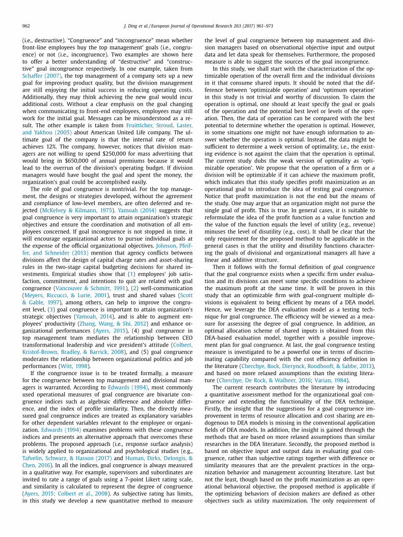
3. Methodology
This part attempts to develop a goal congruence measure for
firms with multiple divisions. Before defining this measure, we in-
vestigate the conditions that optimizable operations of firms and
their subordinate divisions should satisfy. Then, these necessary
conditions will be utilized to devise techniques for achieving our
goal of empirically investigating goal congruence within an organi-
zation.
3.1. Background and notations
We consider firms (denoted as DMUs) that consume both
division-specific inputs and shared inputs to produce multiple out-
puts in D distinct divisions (sub decision making units, SDMUs).
The production process of a DMU with D divisions is shown
in Fig. 1 . For n DMUs, each DMU j ( j = 1 , 2 , . . . , n ) has D divi-
sions, SDM U dj (d = 1 , 2 , . . . , D ) . Let us take two divisions as an ex-
ample. Cook et al. (20 0 0) study the sales and service functions
within the branches of a bank. The variable x dj = (x d 1 j
, x d 2 j
, . . . , x d mdj
)
indicates m d inputs dedicated to SDM U dj , X s j = (X s
1 j , X s
2 j , . . . , X s
l j )
indicates l inputs shared by all SDM U dj (d = 1 , 2 , . . . , D ) . y dj =(y d
1 j , y d
2 j , . . . , y d
tdj ) indicates t d outputs produced exclusively by
SDM U dj (d = 1 , 2 , . . . D ) .
We also define the price vector for division-specific
resources x dj as v dj = (v d 1 j
, v d 2 j
, . . . , v d mdj
)(d = 1 , 2 , . . . , D ) .
s j
= (V s 1 j
, V s 2 j
, . . . , V s l j ) is the price vector for shared inputs.
The price vector for output products y dj are defined as
u dj = (u d 1 j
, u d 2 j
, . . . , v d tdj
) . However, all prices for input and out-
puts are assumed to be unknown, and the shadow prices shall be
determined in the sequel. Just as Chen and Zhu (2011 ) notice that
price information can often be incomplete in practice. Thus, the
models are particularly suitable for applications where price in-
formation is totally absent or partially available. In the latter case,
the prices defined here can be viewed as the relative importance
of the corresponding inputs (or outputs) with respective to the
rest of the inputs (or outputs). For example, prices for inputs, e.g.,
transport, overheads costs of the studied company, are unknown
in Cherchye et al. (2013) , and prices for outputs of bank branches,
e.g., retirement savings plan openings, mortgage accounts opened,
are also not disclosed in Cook et al. (20 0 0) .
Production possibility set contains all input and output com-
binations such that the input ( x dj , X s j ) that can produce y dj (d =
1 , 2 , . . . , D ) for DMU j . In this paper, we assume all observed data
belong to the production possibility set. Furthermore, we as-
sume that the production possibility set exhibits locally strong
Fig. 1. An Example of multi-division production process.
t
t
a
m
c
C
f
D
d
t
j
p
t
T
m
t
l
isposability, locally constant returns-to-scale (CRS), and convexity.
ere, locally CRS implies (d x, d y ) = δ( x, y )( ∀ δ ∈ (−ε , ε ) ) is a pos-
ible direction, where ε is a small positive quantity. Locally strong
isposability means (d x, 0) and (0 , d y ) are feasible adjusting direc-
ion where d x ≥ 0 and d y ≤ 0 . Below we refer to these assumptions
s regular conditions.
The input requirement set of a DM U j ( j = 1 , 2 , . . . , n ) , given out-
ut vectors y j = ( y 1 j , y 2 j , . . . , y D j ) , is defined as:
( y j )
=
{( x 1 j , x 2 j , . . . , x D j , X
s j ) | ( x dj , X
s j ) canproduce y dj , d = 1 , 2 , . . . , D
}
In addition to the above regular conditions, for each output vec-
or y , the input requirement set is assumed to be closed. Before
mbarking on the modeling of optimizable operation for a multi-
ivision firm, we firstly analyze a single division firm.
.2. Single division firm
In firms with a single division, no shared inputs are involved,
nd top management is also the division manager. Thus, no incon-
ruence issue within firm needs to be considered between the two
arties.
The structure of a single-division production process is shown
n Fig. 2 . Here, x j = (x 1 j
, x 2 j
, . . . , x m j
) and y j = (y 1 j
, y 2 j
, . . . , y t j
)
re inputs and outputs for DM U j . v j = (v 1 j
, v 2 j
, . . . , v m j
) and u j =(u
1 j , u
2 j , . . . , u
t j ) are prices for inputs and outputs respectively.
In empirical applications, the production technology of DM U j is
ypically unobserved. In non-parametric production analysis, pro-
uction technology is characterized through the observed set of
nput-output combinations. The input requirement set with re-
pect to y j of DM U j in the one single division case is I( y j ) = ( x j | x j can produce y j } .
To simplify our analysis, we assume that profit maximization is
he only goal of organizations. Even though an organization may
mphasize multiple goals, such as profitability, market position,
roductivity, product leadership, personnel development, public re-
ponsibility ( Feltham and Xie, 1994 ; Yamoah, 2014 ), the main ob-
ective of a firm is profit maximization in the neoclassical theory of
he firm ( Beattie, Taylor, & Watts, 1985 ). We shall discuss the ex-
ension to other situations in the conclusion part of this paper. This
ssumption also holds in the analyses of the organizations with
ultiple divisions.
McFadden (1978) defined a revenue function as R ( u j , x j ) and a
ost function as C( v j , y j ) , so the profit function is π = R ( u j , x j ) −( v j , y j ) . Let us assume that revenue and cost functions are dif-
erentiable. Now let ( x 0 , y 0 ) be the input and output levels of
MU 0 . If a DMU 0 gains the locally maximum profit, it follows that
π | ( x 0 , y 0 ) = R x 0 d x − C y 0 d y ≤ 0 under the constraints of a produc-
ion possibility set, where d x , d y are small technically feasible ad-
ustment to x 0 and y 0 , R x 0 =
∂π∂x
| x 0 , C y 0 =
∂π∂y
| y 0 . This means that the
rofit can no longer be improved locally. We have the following
heorem.
heorem 1. With the regular conditions hold true, DMU 0 gains the
aximum profit, if and only if there exist R x 0 ≥ 0 , C y 0 ≥ 0 , such
hat R x 0 x 0 − C y 0 y 0 = 0 and R x 0 x j − C y 0 y j ≥ 0 hold for all ( x j , y j ) be-
onging to the production possibility set.
J. Ding et al. / European Journal of Operational Research 263 (2017) 961–973 965
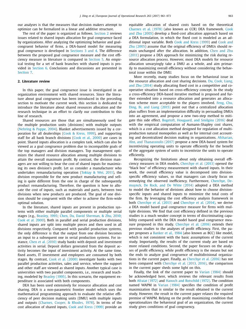
Fig. 3. Division’s production process in a multi-division DMU.
P
l
t
v
b
c
t
l
1
p
s
t
p
a
m
i
t
D
w
o
t
0
a
i
o
c
i
e
P
P
a
p
b
a
t
3
d
p
s
1
p
o
p
∑
f
1
S
c
i
i
2
t
W
h
C
d
s
S
t
i
o
f
e
T
T
g
R∑
f
f
s
o
D
w
D
o
1
∑
4
t
s
H
m
d
d
a
o
t
g
s
t
c
i
i
e
r
a
roof. See the Appendix.
Note that The condition named WAPM from Varian (1984) says
iterally there exist a conical production set Y that p -rationalizes
he data is equivalent to 0 = p i y i ≥ p i y j (for all i, j = 1,…, n ). This is
ery similar to Theorem 1 . However, the result in Varian (1984) is
ased on the definition of p i y i ≥ p i y j (for all i, j = 1,…, n ) and the
onical production set assumption, while Theorem 1 is based on
he premise that dπ ≤ 0 and DMU 0 under examination possesses
ocally CRS and a convex production set. In other words, Theorem
requires the production bundle of DMU 0 can be adjusted pro-
ortionately locally and the shape of the production possibility
et including DMU 0 and other DMUs is some convex set no mat-
er it is a cone or not. Therefore, Theorem 1 relaxes the required
remise in using WAPM. Now we proceed to define an optimiz-
ble operation of DMU 0 . Since attaining maximum profit is the pri-
ary organization-level goal, DMU 0 is optimizable if its operation
n terms of inputs and outputs is consistent with profit maximiza-
ion, which is stated in detail in Definition 1 .
efinition 1. For all the production units DM U j ( j = 1 , 2 , . . . , n )
ith inputs-outputs combinations ( x j , y j ) , we say that DMU 0 is
ptimizable if it can achieve maximum profit, in other words
here exists a price vector ( R x 0 , C y 0 ) , that satisfies R x 0 x 0 − C y 0 y 0 = , R x 0 x j − C y 0 y j ≥ 0( j � = 0) , R x 0 ≥ 0 , C y 0 ≥ 0 .
In the literature, the CCR DEA model for DMU 0 is represented
s max z =
μy 0 ω x 0
, s.t. μy j ω x j
≤ 1 , j = 1 , 2 , . . . , n , where (μ, ω) ≥ 0 . Then,
t is easy to see that the condition for the operation of a DMU to be
ptimizable is equal to the condition for the DMU to be CCR effi-
ient. It is worthy of noting that hereafter the “CCR efficient” qual-
fication means the Farrell efficiency. It is also known as “weakly
fficient”.
roposition 1. An optimizable DM U 0 is CCR efficient, vice versa.
roof. See the Appendix.
In summary, we conclude that DMU 0 is optimizable if it can
chieve profit maximization, and if DMU 0 achieves the maximal
rofit, DMU 0 is CCR efficient or efficient in short. If a DMU cannot
e optimized, it is inefficient in production. Proposition 1 provides
new perspective to the understanding of the CCR efficiency in
he literature.
.3. Multi-division firm
In multi-division firms, D distinct divisions consume both
ivision-specific inputs and shared inputs to produce multiple out-
uts for the company. In turn, the cost of shared inputs, of course,
hould be shared among all divisions.
An example of multi-output production process is shown in Fig.
. For the purpose of illustration, we use Fig. 3 where only the
roduction process of one SDMU is shown. SDM U dj (d = 1 , 2 , . . . , D )
f DM U j consumes both division-specific inputs x dj and shared in-
uts X s j
to produce outputs y dj . However, the cost of shared inputs
D d=1
V s dj
X s j
has to be allocated among all divisions, which is dif-
erent from the single division case. Here V s dj
= (V d 1 j
, V d 2 j
, . . . , V d l j )(d =
, 2 , . . . , D ) with
∑
D d=1
V s dj
= V s j
are the division-specific prices that
DM U dj of DM U j would like to pay for the shared inputs. The total
ost all SDMUs willing to pay equals to the market price of shared
nputs from our modeling perspective. It should be noted that this
mplicit condition will be tested empirically in Section 4 .
V s dj
(d = 1 , 2 , . . . , D ) is also called implicit prices ( Cherchye et al.,
013 ), which represents the fraction of the aggregated prices of
he shared inputs that are borne by different production divisions.
hen consuming shared inputs, however, DMUs generally do not
ave the complete knowledge about the usage among divisions.
onsequently, a mechanism is needed to split shared inputs across
ivisions. In this research, we use a ratio βdj
= (βd 1 j
, βd 2 j
, . . . , βd l j ) in-
tead of V s dj
, where V s dj
= βdj V s j , to represent the partial price that
DM U dj of DM U j would like to pay for the shared input. The ra-
io is more flexible in a sense that when the quantity of a shared
nput, say X s j , is of interest, we can apply allocation ratios to X s
j to
btain the quantity that a SDMU consumes.
Assuming the profit function of a multi-division DMU takes the
orm π =
∑
D d=1
R d ( u dj , x dj , X s j ) − ∑
D d=1
C d ( v dj , V s
dj , y dj ) , and is differ-
ntiable with respect to x dj , X s j , y dj given u dj , v dj , and V s
dj , we have
heorem 2 below by following the same logic of Theorem 1 .
heorem 2. With the regular conditions hold true, DM U 0
ains the maximum profit, if and only if there exist R X s 0
≥ 0 ,
x d0 ≥ 0 , C y d0
≥ 0(d = 1 , 2 , . . . , D ) such that ∑
D d=1
R x d0 x d0 + R X s
0 X s
0 −
D d=1
C y d0 y d0 = 0 , and
∑
D d=1
R x d0 x dj + R X s
0 X s
j − ∑
D d=1
C y d0 y dj ≥ 0 hold
or all ( x dj , X s j , y dj ) belonging to the production possibility set.
Here, R X s 0 , R x d0
, and C y d0 are first partial derivatives of the profit
unction with respect to X s 0 , x d0 , and y d0 respectively. On the ba-
is of Theorem 2 , we extend Definition 1 to a new definition of
ptimizable operation for a multi-division firm as follows.
efinition 2. For all the production units DM U j ( j = 1 , 2 , . . . , n )
ith inputs-outputs combinations ( x dj , X s j , y dj )(d = 1 , 2 , . . . , D ) ,
MU 0 is optimizable if it can achieve maximum profit. In
ther words, there exists a price vector ( R x d0 , R X s
0 , C y d0
)(d = , 2 , . . . , D ) that satisfies
∑
D d=1
R x d0 x d0 + R X s
0 X s
0 − ∑
D d=1
C y d0 y d0 = 0 ,
D d=1
R x d0 x dj + R X s
0 X s
j − ∑
D d=1
C y d0 y dj ≥ 0( j � = 0) .
. Measure of goal congruence
Suppose that the top management of a firm only cares about
he maximum profit gained from the investment of shared re-
ources, shared resources are allocated committing to this goal.
owever, due to divergence of interests between the top manage-
ent and division managers and the fact that the benefits that a
ivision derived from shared inputs is the private information of
ivision managers, the allocation plan preferred by the top man-
gement might be in conflict with division managers’ optimizable
peration. In other words, goal incongruence may be present be-
ween the top management and division managers.
To complete the task of testing quantitatively whether
oal congruence between top management and divi-
ion managers exists, our logic is to hypothesize that
he division managers and top management are goal
ongruent in the first place. An implication of this hypothesis
s that division managers are willing to accept any allocation plan
n the best interest of the overall firm. Then, based on empirical
vidence, we shall decide whether the congruence hypothesis is
ejected or not. The definition of goal congruence between a DMU
nd its SDMUs is provided in Definition 3 .
966 J. Ding et al. / European Journal of Operational Research 263 (2017) 961–973
S
t
l
(
a
i
t
m
r
C
i
ω
w
(
ω
o
r
c
a
v
L
i
P
n
1
a
i
t
t
P
b
a
t
a
o
e
c
t
a
b
D
fi
e
s
Definition 3. If a focal DMU and its SDMUs can achieve max-
imum profit at the same time, then they are goal congru-
ent. SDMU d 0 with inputs-outputs combinations ( x d0 , X s 0 , y d0 )(d =
1 , 2 , . . . , D ) of DMU 0 is optimizable if it can achieve maxi-
mum profit in the following sense: there exists a price vector
( R x d0 , R X s
0 , C y d0
) and βd0
= (βd 10
, βd 20
, . . . , βd l0
)(d = 1 , 2 , . . . , D ) , such
that R x d0 x d0 + βd0 R X s
0 X s
0 − C y d0
y d0 = 0 , R x d0 x dj + βd0 R X s
0 X s
j − C y d0
y dj ≥0( j � = 0) ,
∑
D d=1
βd0 = 1 , βd0 ≥ 0 , for d = 1 , 2 , . . . , D . Here, βd0 R X s 0 X s
j
indicates the partial cost that SDMU d 0 of DM U j pay for the shared
input.
Note that in the conditions of Definition 3 , SDM U d0 of DMU 0
only compares with the corresponding SDM U dj ( j � = 0) of other
DM U j ( j � = 0) . If the DMU and SDMUs are not goal congruent, there
are two causes that prevent the DMU and SDMUs becoming opti-
mizable simultaneously. The first is that the operations of SDMUs
are not optimizable themselves (denoted Cause 1 for latter refer-
ence). This is because they are inefficient in production. This ex-
planation is the same as that in the single division setting. The
other is that if the SDMUs can be optimizable except for the over-
all DMU, and then there exist differences in input and output pri-
orities and shared resources usage among the SDMUs and DMU
(denoted Cause 2 for latter reference). We now proceed to propose
models to capture quantitatively the magnitude of goal incongru-
ence embodying those two causes.
Beasley (1995) proposes a DEA model assuming CRS for max-
imizing the overall efficiency, which can determine the joint effi-
ciency of all production processes (see model ( 1 )). Note that the
term ‘overall efficiency’ here emphasizes it is the efficiency of the
entire DMU consisting of many DMUs, while the term ‘joint effi-
ciency’ highlights that the overall efficiency can be interpreted as
the aggregation of SDMU efficiencies (i.e., the weighted average
of SDMU efficiencies) . Below, we explore the implication of this
model for measuring the degree of goal congruence, which has not
yet been discussed in the literature.
max z =
∑
D d=1
μd0 y d0
ω 0 X
s 0
+
∑
D d=1
ω d0 x d0
s.t. μ10 y 1 j
β10 ω 0 X
s j + ω 10 x 1 j
≤ 1 , j = 1 , 2 , . . . , n
μ20 y 2 j
β20 ω 0 X
s j + ω 20 x 2 j
≤ 1 , j = 1 , 2 , . . . , n
. . .
μD 0 y D j
βD 0 ω 0 X
s j + ω D 0 x D j
≤ 1 , j = 1 , 2 , . . . , n
∑
D d=1 βd0 = 1
ω 0 ≥ 0 , βd0 ≥ 0 , μd0 ≥ 0 , ω d0 ≥ 0 , d = 1 , 2 , . . . , D, j = 1 , 2 , . . . , n
(1)
In model ( 1 ), each DMU is evaluated in its most favor-
able light. Hence, each DMU is allowed to choose a set of
( βd0 , ω 0 , ω d0 , μd0 ) to maximize its efficiency score. The objec-
tive function of model ( 1 ) is an overall efficiency measure of
DMU 0 , The efficiency for each SDMU of DMU 0 is measured byμd0 y d0
βd0 ω 0 X s 0 + ω d0 x d0
(d = 1 , 2 , . . . , D ) . In other words, SDMU’s efficiency is
defined based on a specific allocation of shared inputs among SD-
MUs. One should be cautious in understanding the phrase “SDMU’s
efficiency”. As the realistic consumption data of shared inputs can-
not be observed, it is difficult to evaluate the performance of a
SDMU. Here, the efficiency of a SDMU is defined as a ratio of
weighted outputs to weighted inputs. However, these weights are
given aiming at putting the DMU as a whole, rather than the
DMU, in the best possible light. This is not quite consistent with
he conventional definition of efficiency of a DMU in the DEA
iterature. Consequently, we refer to the objective value of model
1 ) as the overall efficiency of a DMU and the efficiency of a SDMU
s the divisional efficiency of a SDMU. The use of overall efficiency
nstead of ‘CCR efficiency’ or efficiency in the multi-division case is
o highlight the difference between model ( 1 ) and the classic CCR
odel. A DMU or SDMU will be overall or divisional efficient if the
espective efficiency achieves 1.
By adopting “Charnes-Cooper” transformation ( Charnes &
ooper, 1962 ), the objective function of model ( 1 ) can be expressed
n a non-ratio form. In addition, we make the change of variables
d 0 = βd0 ω 0 (d = 1 , 2 , . . . , D ) , in which ω
d 0 has the same dimension
ith ω 0 , and then model ( 1 ) is transformed into a linear model
2 ).
max z =
∑
D d=1 μd0 y d0
s.t. μ10 y 1 j − ω
1 0 X
s j − ω 10 x 1 j ≤ 0 , j = 1 , 2 , . . . , n
μ20 y 2 j − ω
2 0 X
s j − ω 20 x 2 j ≤ 0 , j = 1 , 2 , . . . , n
. . .
μD 0 y D j − ω
D 0 X
s j − ω D 0 x D j ≤ 0 , j = 1 , 2 , . . . , n
∑
D d=1 ω
d 0 = ω 0
ω 0 X
s 0 +
∑
D d=1 ω d0 x d0 = 1
0 ≥ 0 , ω
d 0 ≥ 0 , μd0 ≥ 0 , ω d0 ≥ 0 , d = 1 , 2 , . . . , D, j = 1 , 2 , . . . , n
(2)
In model ( 2 ), it is clear that there are differences in input and
utput priorities and shared resources usage for the SDMUs (rep-
esented in inputs and outputs weights) if the DMU and SDMUs
annot be optimizable at the same time. The relationship between
DMU’s overall efficiency and SDMUs’ divisional efficiencies is re-
ealed in Lemma 1 .
emma 1. A necessary condition for DMU 0 to be overall efficient
s that all SDMU d 0 of DMU 0 are divisional efficient.
roof. See Appendix.
Lemma 1 supports the Cause 1 why the DMU and SDMUs can-
ot be optimizable at the same time. The necessity of Lemma
shows that SDMUs are not efficient in production when the over-
ll DMU is not optimizable. A single division DMU is optimizable
f it is CCR efficient according to Proposition 1 . However, an addi-
ional condition is required for multi-division firms. We summarize
he condition in Proposition 2 .
roposition 2. The sufficient and necessary condition for DMU 0 to
e overall efficient is that it is optimizable and multiple divisions
re goal-congruent with it.
The non-sufficiency of Lemma 1 and Proposition 2 verify that
here are conflicts in determination of input and output priorities
nd the shared resources usage (represented by the inputs and
utputs weights in model ( 2 )) even though the two SDMUs are
fficient, which supports the Cause 2 why the DMU and SDMUs
annot be optimizable at the same time. Therefore, if a DMU is op-
imizable and its SDMUs are goal-congruent with it, both the DMU
nd all its SDMUs are able to attain their maximum profit. Then
oth the DMU and all its SDMUs are overall efficient. In turn, if a
MU is overall efficient, and then all its SDMUs are divisional ef-
cient. Furthermore, the DMU and its SDMUs are congruent with
ach other. Hence, DMU’s overall efficiency is a good indicator to
how whether its SDMUs are goal-congruent with it.

J. Ding et al. / European Journal of Operational Research 263 (2017) 961–973 967
e
i
e
a
l
I
c
l
o
β
b
i
e
m
i
b
f
u
S
i
q
t
fi
w
o
1
b
o
5
e
a
(
i
i
t
r
b
i
a
t
f
5
w
D
D
1
(
(
x
d
p
y
t
f
D
i
t
�
t
a
i
P
e
P
w
u
w
v
5
D
c
e
a
t
(
(
p
p
o
a ∑
t
s
d
v
D
s
fi
(
c
m
m
fi
F
a
T
c
e
t
o
a
m
In addition to serving as an indicator of whether goal congru-
nce is achieved, a DMU’s overall efficiency measure by model ( 1 )
s a measure of the degree of goal congruence. As a DMU’s overall
fficiency is a weighted average of each SDMU’s efficiency (under
specific shared input allocation scheme) ( Beasley, 1995 ), SDMUs’
ow efficiency level will lead to a smaller overall efficiency score.
n this case, it is obviously that SDMUs and the DMU are goal in-
ongruent. Furthermore, the lower the efficiencies of SDMUs, the
ower the degree of congruence is.
The overall efficiency proposed here sheds light on the source
f goal incongruence. For example, in model ( 1 ), the variables
d0 (d = 1 , 2 , . . . , D ) are treated as DMU-specific variables. It will
e at the discretion of the DMU under evaluation to allocate shared
nputs among its divisions. However, as long as one SDMU is not
fficient under DMU’s allocation scheme for achieving the profit
aximization goal, the overall DMU cannot be efficient. If there
s no allocation scheme available to reconcile the profit optimizing
ehaviors of both SDMUs and DMU as a whole, goal in-congruence
ollows.
If SDMUs are to adjust their inputs in goal incongruent sit-
ation to achieve a goal congruent state, the extent to which a
DMU needs to make adjustment in order to be overall efficient
s reflected in model ( 1 ). Treating the overall DMU efficiency as a
uantitative measure for goal congruence constitutes a contribu-
ion of this research. The goal congruence measure, other than ef-
ciency measure, offers a new insight to the optimal value of the
eighted ratio efficiency in model ( 1 ). In the course of maximizing
verall efficiency of a DMU, a set of optimal βdj (d = 1 , 2 , . . . , D ; j = , 2 , . . . , n ) is obtained. As a result, a measure of goal congruence
etween the DMUs and their SDMUs is provided, together with an
ptimal allocation scheme of the shared resources.
. Relationship between goal congruence measure and cost
fficiency
The allocation of shared inputs among divisions of a DMU has
lready been studied by Cherchye et al. (2013) and Cherchye et al.
2014) . They propose a structural DEA approach to model cost min-
mizing behavior at the overall firm level when allocating shared
nputs among divisions. A notion of cost efficiency is developed in
hese two studies. Adopting the notations in the current paper, we
e-write the cost efficiency definition as Definitions 4 and 5 for
oth the single division firms and multi-division firms. Cost min-
mization and cost efficiency is an important topic of budgeting
nd management control as well. Hence, the difference between
he overall efficiency indicated in model ( 1 ) and cost efficiency is
urther discussed in this section.
.1. Single-division firm
Based on the cost efficiency defined by Cherchye et al. (2013) ,
e have the following cost efficiency definition.
efinition 4. Let v 0 be the prices for y 0 and x 0 respectively.
MU 0 with a single division is cost efficient among all DM U j ( j = , 2 , . . . , n ) if and only if there exists prices v 0 that satisfy:
1) x j ∈ I( y j ) , j = 1 , 2 , . . . , n ;
2) v 0 x 0 = min
j∈ �0
v 0 x j , where j ∈ �0 = { i | y i ≥ y 0 } .
In this definition, the first constraint guarantees that the inputs
j can effectively produce the outputs y j under price v 0 , which in-
icates technology feasibility. v 0 x 0 = min v 0 x j ensures that DMU 0
roduce y 0 at a minimal cost under price v 0 . For these DM U j with
j < y 0 , by definition, the cost v 0 x j incurred to produce y j is less
han or equal to v 0 x 0 for producing y 0 , otherwise more inputs
or DM U j indicates inefficiency. Both of these two cases infer that
MUs with y j < y 0 are meaningless for comparison purpose. Such
s also in line with the free output disposability of production func-
ions that less output never requires more input. Therefore, the set
0 = { i | y i ≥ y 0 } is built to capture those DM U j that produce at least
he output y 0 . We know that an optimizable DMU is CCR efficient
ccording to Proposition 1 . Furthermore, if a DMU is CCR efficient,
t follows the Proposition 3 below.
roposition 3. If DM U 0 is CCR efficient, and then DMU 0 is cost
fficient.
roof. See the Appendix.
However, if DMU 0 is cost efficient, CCR efficiency cannot al-
ays be inferred. For those DM U j having y j ≥ y 0 , by setting a small
0 ( u 0 ≥ 0) , which satisfies u 0 y j − u 0 y 0 ≤ ( min v 0 x j ) − v 0 x 0 ( j ∈ �) ,
e have v 0 x 0 − u 0 y 0 ≤ v 0 x j − u 0 y j . There is no evidence that
0 x 0 − u 0 y 0 = 0 . Therefore, DMU 0 is CCR efficient cannot hold.
.2. Multiple-division firm
efinition 5. For a multiple-division DMU 0 with inputs-outputs
ombinations ( x d0 , X s 0 , y d0 )(d = 1 , 2 , . . . , D ) , it is multi-output cost
fficient among all DM U j ( j = 1 , 2 , . . . , n ) if and only if there exist
set of prices ( v dj , V s j ) and βd0 = (βd
10 , βd
20 , . . . , βd
l0 )(d = 1 , 2 , . . . , D )
hat satisfy:
1) ( x d0 , X s 0 ) ∈ I( y d0 )
2) v d0 x d0 + βd0 V s 0
X s 0
= min
j∈ �d 0 ( v d0 x dj + βd0 V
s 0
X s j ) ,
∑
D d=1
βd0 = 1 ,
where j ∈ �d 0
= { i | y di ≥ y d0 } , d = 1 , 2 , . . . , D .
In this definition, the first constraint guarantees that the in-
uts ( x d0 , X s 0 ) can effectively produce the outputs y d0 under the
rice ( v d0 , βd0 V s 0 ) , which indicates technology feasibility. The sec-
nd constraint ensures that every SDM U d0 of DMU 0 produce y d0
t a minimal cost under the price ( v d0 , βd0 V s 0 ) . The constraint
D d=1
βd0 = 1 confines the money paid for shared inputs to meet
he total price requirement. Same as that in Definition 4 , the
et �d 0
= { i | y di ≥ y d0 } indicates that only these SDM U dj that pro-
uce at least y d0 are compared with SDMU d 0 . Note that each di-
ision SDMU d 0 of DMU 0 should satisfies the second constraint of
efinition 5 . Thus there are actually D sub-constraints within the
econd constraint. If all SDMUs of DMU 0 are measured as cost ef-
cient, it is obviously that DMU 0 is cost efficient.
The cost efficiency measure proposed in Cherchye et al.
2013) is shown as follows.
C E 0 = max
∑
D d=1
c d 0
V
s 0
X
s 0
+
∑
D d=1
v d0 x d0
d 0 ≤ v d0 x dj + βd0 V
s 0 X
s j , j ∈ �d
0 = { i | y di ≥ y d0 } , d = 1 , 2 , · · ·, D
∑
D d=1 βd0 = 1
(3)
Note that parameters c d 0 (d = 1 , 2 , . . . , D ) in model ( 3 ) represent
in
j∈ �d 0 ( v d0 x dj + βd0 V
s 0
X s j ) . It is easy to verify that cost efficiency
easurement for a DMU in model ( 3 ) is equivalent to the cost ef-
cient definition in Definition 5 when the DMU is cost efficient.
irst, if a DMU 0 is cost efficient as defined in Definition 5 , then
ll its SDMUs are cost efficient, and we get c d 0 = v d0 x d0 + βd0 V
s 0
X s 0 .
hus the objective function of model ( 3 ) equals to one, and all
onstraints of model ( 3 ) are satisfied. Second, if CE 0 of model ( 3 )
quals to one, and then
∑
D d=1
c d 0 =
∑
D d=1
v d0 x d0 + βd0 V s 0
X s 0 . Suppose
here exists one c p 0
for SDM U p0 equal to v p0 x pk + βp0 V s 0
X s k (k ∈ S
p 0 )
ther than v p0 x p0 + βp0 V s 0
X s 0 . It follows that c
p 0
< v p0 x p0 + βp0 V s 0
X s 0 ,
nd
∑
D d=1
c d 0 <
∑
D d=1
v d0 x d0 + βd0 V s 0
X s 0 , which contradicts that CE 0 of
odel ( 3 ) equals to one Through the contradiction, we know that
968 J. Ding et al. / European Journal of Operational Research 263 (2017) 961–973
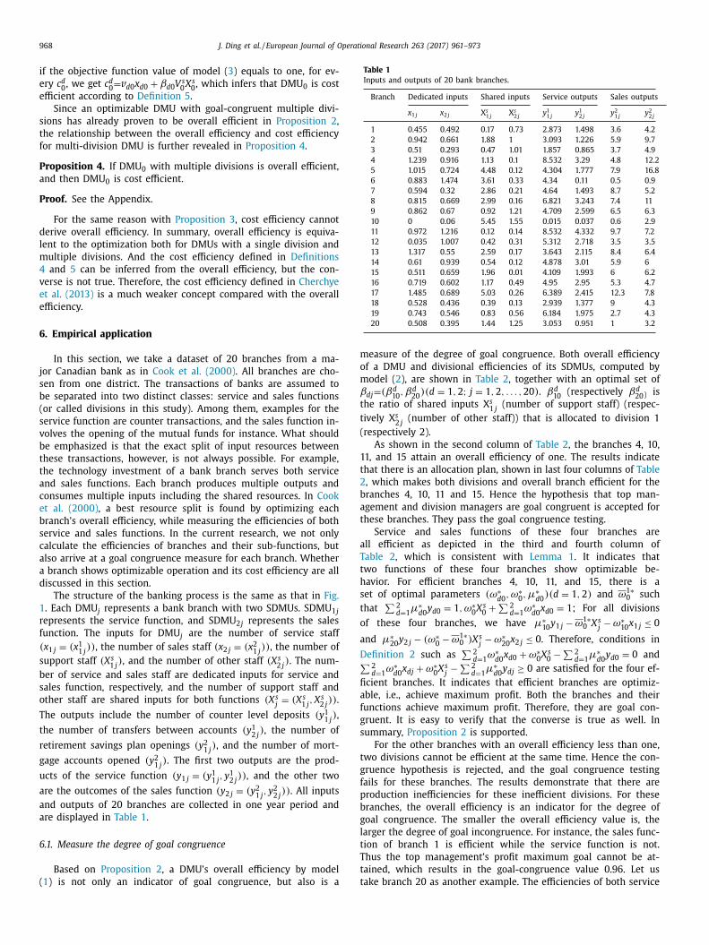
Table 1
Inputs and outputs of 20 bank branches.
Branch Dedicated inputs Shared inputs Service outputs Sales outputs
x 1 j x 2 j X s 1 j
X s 2 j
y 1 1 j
y 1 2 j
y 2 1 j
y 2 2 j
1 0.455 0.492 0.17 0.73 2.873 1.498 3.6 4.2
2 0.942 0.661 1.88 1 3.093 1.226 5.9 9.7
3 0.51 0.293 0.47 1.01 1.857 0.865 3.7 4.9
4 1.239 0.916 1.13 0.1 8.532 3.29 4.8 12.2
5 1.015 0.724 4.48 0.12 4.304 1.777 7.9 16.8
6 0.883 1.474 3.61 0.33 4.34 0.11 0.5 0.9
7 0.594 0.32 2.86 0.21 4.64 1.493 8.7 5.2
8 0.815 0.669 2.99 0.16 6.821 3.243 7.4 11
9 0.862 0.67 0.92 1.21 4.709 2.599 6.5 6.3
10 0 0.06 5.45 1.55 0.015 0.037 0.6 2.9
11 0.972 1.216 0.12 0.14 8.532 4.332 9.7 7.2
12 0.035 1.007 0.42 0.31 5.312 2.718 3.5 3.5
13 1.317 0.55 2.59 0.17 3.643 2.115 8.4 6.4
14 0.61 0.939 0.54 0.12 4.878 3.01 5.9 6
15 0.511 0.659 1.96 0.01 4.109 1.993 6 6.2
16 0.719 0.602 1.17 0.49 4.95 2.95 5.3 4.7
17 1.485 0.689 5.03 0.26 6.389 2.415 12.3 7.8
18 0.528 0.436 0.39 0.13 2.939 1.377 9 4.3
19 0.743 0.546 0.83 0.56 6.184 1.975 2.7 4.3
20 0.508 0.395 1.44 1.25 3.053 0.951 1 3.2
m
o
m
β
t
t
(
1
t
2
b
a
t
a
T
t
h
s
t
o
a
D ∑
fi
a
f
g
s
t
g
f
p
b
g
l
t
T
t
t
if the objective function value of model ( 3 ) equals to one, for ev-
ery c d 0
, we get c d 0 = v d0 x d0 + βd0 V
s 0
X s 0 , which infers that DMU 0 is cost
efficient according to Definition 5 .
Since an optimizable DMU with goal-congruent multiple divi-
sions has already proven to be overall efficient in Proposition 2 ,
the relationship between the overall efficiency and cost efficiency
for multi-division DMU is further revealed in Proposition 4 .
Proposition 4. If DMU 0 with multiple divisions is overall efficient,
and then DMU 0 is cost efficient.
Proof. See the Appendix.
For the same reason with Proposition 3 , cost efficiency cannot
derive overall efficiency. In summary, overall efficiency is equiva-
lent to the optimization both for DMUs with a single division and
multiple divisions. And the cost efficiency defined in Definitions
4 and 5 can be inferred from the overall efficiency, but the con-
verse is not true. Therefore, the cost efficiency defined in Cherchye
et al. (2013) is a much weaker concept compared with the overall
efficiency.
6. Empirical application
In this section, we take a dataset of 20 branches from a ma-
jor Canadian bank as in Cook et al. (20 0 0) . All branches are cho-
sen from one district. The transactions of banks are assumed to
be separated into two distinct classes: service and sales functions
(or called divisions in this study). Among them, examples for the
service function are counter transactions, and the sales function in-
volves the opening of the mutual funds for instance. What should
be emphasized is that the exact split of input resources between
these transactions, however, is not always possible. For example,
the technology investment of a bank branch serves both service
and sales functions. Each branch produces multiple outputs and
consumes multiple inputs including the shared resources. In Cook
et al. (20 0 0) , a best resource split is found by optimizing each
branch’s overall efficiency, while measuring the efficiencies of both
service and sales functions. In the current research, we not only
calculate the efficiencies of branches and their sub-functions, but
also arrive at a goal congruence measure for each branch. Whether
a branch shows optimizable operation and its cost efficiency are all
discussed in this section.
The structure of the banking process is the same as that in Fig.
1 . Each DMU j represents a bank branch with two SDMUs. SDMU 1 j
represents the service function, and SDMU 2 j represents the sales
function. The inputs for DMU j are the number of service staff
( x 1 j = (x 1 1 j
)) , the number of sales staff ( x 2 j = (x 2 1 j
)) , the number of
support staff (X s 1 j
) , and the number of other staff (X s 2 j
) . The num-
ber of service and sales staff are dedicated inputs for service and
sales function, respectively, and the number of support staff and
other staff are shared inputs for both functions (X s j = (X s
1 j , X s
2 j )) .
The outputs include the number of counter level deposits (y 1 1 j
) ,
the number of transfers between accounts (y 1 2 j
) , the number of
retirement savings plan openings (y 2 1 j
) , and the number of mort-
gage accounts opened (y 2 1 j
) . The first two outputs are the prod-
ucts of the service function ( y 1 j = (y 1 1 j
, y 1 2 j
)) , and the other two
are the outcomes of the sales function ( y 2 j = (y 2 1 j
, y 2 2 j
)) . All inputs
and outputs of 20 branches are collected in one year period and
are displayed in Table 1 .
6.1. Measure the degree of goal congruence
Based on Proposition 2 , a DMU’s overall efficiency by model
( 1 ) is not only an indicator of goal congruence, but also is a
easure of the degree of goal congruence. Both overall efficiency
f a DMU and divisional efficiencies of its SDMUs, computed by
odel ( 2 ), are shown in Table 2 , together with an optimal set of
dj = (βd 10
, βd 20
)(d = 1 , 2 ; j = 1 , 2 , . . . , 20) . βd 10
(respectively βd 20 )
is
he ratio of shared inputs X
s 1 j
(number of support staff) (respec-
ively X
s 2 j
(number of other staff)) that is allocated to division 1
respectively 2).
As shown in the second column of Table 2 , the branches 4, 10,
1, and 15 attain an overall efficiency of one. The results indicate
hat there is an allocation plan, shown in last four columns of Table
, which makes both divisions and overall branch efficient for the
ranches 4, 10, 11 and 15. Hence the hypothesis that top man-
gement and division managers are goal congruent is accepted for
hese branches. They pass the goal congruence testing.
Service and sales functions of these four branches are
ll efficient as depicted in the third and fourth column of
able 2 , which is consistent with Lemma 1 . It indicates that
wo functions of these four branches show optimizable be-
avior. For efficient branches 4, 10, 11, and 15, there is a
et of optimal parameters (ω
∗d0
, ω
∗0 , μ
∗d0
)(d = 1 , 2) and ω
1 ∗0 such
hat ∑
2 d=1
μ∗d0
y d0 = 1 , ω
∗0 X
s 0
+
∑
2 d=1
ω
∗d0
x d0 = 1 ; For all divisions
f these four branches, we have μ∗10
y 1 j − ω
1 ∗0 X s
j − ω
∗10
x 1 j ≤ 0
nd μ∗20 y 2 j − (ω
∗0 − ω
1 ∗0 ) X
s j − ω
∗20 x 2 j ≤ 0 . Therefore, conditions in
efinition 2 such as ∑
2 d=1
ω
∗d0
x d0 + ω
∗0 X
s 0
− ∑
2 d=1
μ∗d0
y d0 = 0 and
2 d=1
ω
∗d0
x dj + ω
∗0 X s
j − ∑
2 d=1
μ∗d0
y dj ≥ 0 are satisfied for the four ef-
cient branches. It indicates that efficient branches are optimiz-
ble, i.e., achieve maximum profit. Both the branches and their
unctions achieve maximum profit. Therefore, they are goal con-
ruent. It is easy to verify that the converse is true as well. In
ummary, Proposition 2 is supported.
For the other branches with an overall efficiency less than one,
wo divisions cannot be efficient at the same time. Hence the con-
ruence hypothesis is rejected, and the goal congruence testing
ails for these branches. The results demonstrate that there are
roduction inefficiencies for these inefficient divisions. For these
ranches, the overall efficiency is an indicator for the degree of
oal congruence. The smaller the overall efficiency value is, the
arger the degree of goal incongruence. For instance, the sales func-
ion of branch 1 is efficient while the service function is not.
hus the top management’s profit maximum goal cannot be at-
ained, which results in the goal-congruence value 0.96. Let us
ake branch 20 as another example. The efficiencies of both service
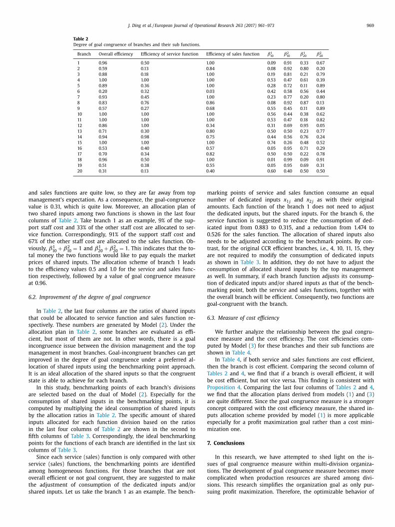
J. Ding et al. / European Journal of Operational Research 263 (2017) 961–973 969
Table 2
Degree of goal congruence of branches and their sub functions.
Branch Overall efficiency Efficiency of service function Efficiency of sales function β1 10 β2
10 β1 20 β2
20
1 0.96 0.50 1.00 0.09 0.91 0.33 0.67
2 0.59 0.13 0.84 0.08 0.92 0.80 0.20
3 0.88 0.18 1.00 0.19 0.81 0.21 0.79
4 1.00 1.00 1.00 0.53 0.47 0.61 0.39
5 0.89 0.36 1.00 0.28 0.72 0.11 0.89
6 0.20 0.32 0.03 0.42 0.58 0.56 0.44
7 0.93 0.45 1.00 0.23 0.77 0.20 0.80
8 0.83 0.76 0.86 0.08 0.92 0.87 0.13
9 0.57 0.27 0.68 0.55 0.45 0.11 0.89
10 1.00 1.00 1.00 0.56 0.44 0.38 0.62
11 1.00 1.00 1.00 0.53 0.47 0.18 0.82
12 0.86 1.00 0.34 0.31 0.69 0.95 0.05
13 0.71 0.30 0.80 0.50 0.50 0.23 0.77
14 0.94 0.98 0.75 0.44 0.56 0.76 0.24
15 1.00 1.00 1.00 0.74 0.26 0.48 0.52
16 0.53 0.40 0.57 0.05 0.95 0.71 0.29
17 0.70 0.34 0.82 0.50 0.50 0.22 0.78
18 0.96 0.50 1.00 0.01 0.99 0.09 0.91
19 0.51 0.38 0.55 0.05 0.95 0.69 0.31
20 0.31 0.13 0.40 0.60 0.40 0.50 0.50
a
m
v
t
c
p
v
6
v
t
p
t
t
a
6
t
s
a
c
i
m
i
l
I
s
a
c
c
b
i
i
fi
p
c
s
a
o
t
s
m
n
a
t
s
i
0
n
t
a
a
c
a
t
m
t
g
6
e
p
s
t
T
b
P
w
a
c
p
e
m
7
s
t
c
s
s
nd sales functions are quite low, so they are far away from top
anagement’s expectation. As a consequence, the goal-congruence
alue is 0.31, which is quite low. Moreover, an allocation plan of
wo shared inputs among two functions is shown in the last four
olumns of Table 2 . Take branch 1 as an example, 9% of the sup-
ort staff cost and 33% of the other staff cost are allocated to ser-
ice function. Correspondingly, 91% of the support staff cost and
7% of the other staff cost are allocated to the sales function. Ob-
iously, β1 10
+ β2 10
= 1 and β1 20
+ β2 20
= 1 . This indicates that the to-
al money the two functions would like to pay equals the market
rices of shared inputs. The allocation scheme of branch 1 leads
o the efficiency values 0.5 and 1.0 for the service and sales func-
ion respectively, followed by a value of goal congruence measure
t 0.96.
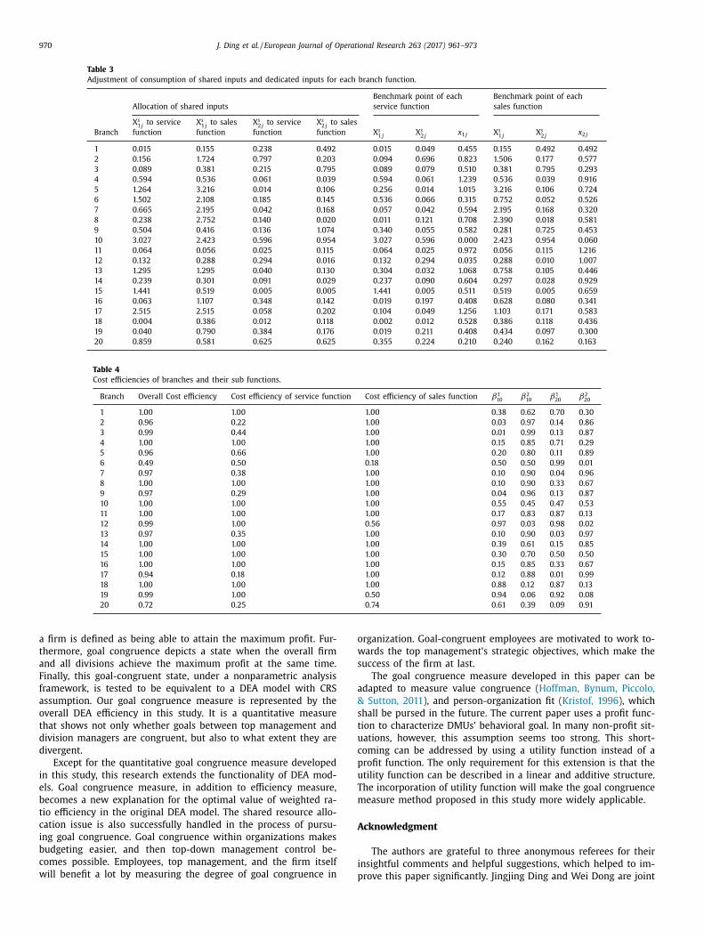
.2. Improvement of the degree of goal congruence
In Table 2 , the last four columns are the ratios of shared inputs
hat could be allocated to service function and sales function re-
pectively. These numbers are generated by Model ( 2 ). Under the
llocation plan in Table 2 , some branches are evaluated as effi-
ient, but most of them are not. In other words, there is a goal
ncongruence issue between the division management and the top
anagement in most branches. Goal-incongruent branches can get
mproved in the degree of goal congruence under a preferred al-
ocation of shared inputs using the benchmarking point approach.
t is an ideal allocation of the shared inputs so that the congruent
tate is able to achieve for each branch.
In this study, benchmarking points of each branch’s divisions
re selected based on the dual of Model ( 2 ). Especially for the
onsumption of shared inputs in the benchmarking points, it is
omputed by multiplying the ideal consumption of shared inputs
y the allocation ratios in Table 2 . The specific amount of shared
nputs allocated for each function division based on the ratios
n the last four columns of Table 2 are shown in the second to
fth columns of Table 3 . Correspondingly, the ideal benchmarking
oints for the functions of each branch are identified in the last six
olumns of Table 3 .
Since each service (sales) function is only compared with other
ervice (sales) functions, the benchmarking points are identified
mong homogeneous functions. For those branches that are not
verall efficient or not goal congruent, they are suggested to make
he adjustment of consumption of the dedicated inputs and/or
hared inputs. Let us take the branch 1 as an example. The bench-
arking points of service and sales function consume an equal
umber of dedicated inputs x 1 j and x 2 j as with their original
mounts. Each function of the branch 1 does not need to adjust
he dedicated inputs, but the shared inputs. For the branch 6, the
ervice function is suggested to reduce the consumption of ded-
cated input from 0.883 to 0.315, and a reduction from 1.474 to
.526 for the sales function. The allocation of shared inputs also
eeds to be adjusted according to the benchmark points. By con-
rast, for the original CCR efficient branches, i.e., 4, 10, 11, 15, they
re not required to modify the consumption of dedicated inputs
s shown in Table 3 . In addition, they do not have to adjust the
onsumption of allocated shared inputs by the top management
s well. In summary, if each branch function adjusts its consump-
ion of dedicated inputs and/or shared inputs as that of the bench-
arking point, both the service and sales functions, together with
he overall branch will be efficient. Consequently, two functions are
oal-congruent with the branch.
.3. Measure of cost efficiency
We further analyze the relationship between the goal congru-
nce measure and the cost efficiency. The cost efficiencies com-
uted by Model ( 3 ) for these branches and their sub functions are
hown in Table 4 .
In Table 4 , if both service and sales functions are cost efficient,
hen the branch is cost efficient. Comparing the second column of
ables 2 and 4 , we find that if a branch is overall efficient, it will
e cost efficient, but not vice versa. This finding is consistent with
roposition 4 . Comparing the last four columns of Tables 2 and 4 ,
e find that the allocation plans derived from models ( 1 ) and ( 3 )
re quite different. Since the goal congruence measure is a stronger
oncept compared with the cost efficiency measure, the shared in-
uts allocation scheme provided by model ( 1 ) is more applicable
specially for a profit maximization goal rather than a cost mini-
ization one.
. Conclusions
In this research, we have attempted to shed light on the is-
ues of goal congruence measure within multi-division organiza-
ions. The development of goal congruence measure becomes more
omplicated when production resources are shared among divi-
ions. This research simplifies the organization goal as only pur-
uing profit maximization. Therefore, the optimizable behavior of
970 J. Ding et al. / European Journal of Operational Research 263 (2017) 961–973
Table 3
Adjustment of consumption of shared inputs and dedicated inputs for each branch function.
Allocation of shared inputs
Benchmark point of each
service function
Benchmark point of each
sales function
Branch
X s 1 j
to service
function
X s 1 j
to sales
function
X s 2 j
to service
function
X s 2 j
to sales
function X s 1 j
X s 2 j
x 1 j X s 1 j
X s 2 j
x 2 j
1 0.015 0.155 0.238 0.492 0.015 0.049 0.455 0.155 0.492 0.492
2 0.156 1.724 0.797 0.203 0.094 0.696 0.823 1.506 0.177 0.577
3 0.089 0.381 0.215 0.795 0.089 0.079 0.510 0.381 0.795 0.293
4 0.594 0.536 0.061 0.039 0.594 0.061 1.239 0.536 0.039 0.916
5 1.264 3.216 0.014 0.106 0.256 0.014 1.015 3.216 0.106 0.724
6 1.502 2.108 0.185 0.145 0.536 0.066 0.315 0.752 0.052 0.526
7 0.665 2.195 0.042 0.168 0.057 0.042 0.594 2.195 0.168 0.320
8 0.238 2.752 0.140 0.020 0.011 0.121 0.708 2.390 0.018 0.581
9 0.504 0.416 0.136 1.074 0.340 0.055 0.582 0.281 0.725 0.453
10 3.027 2.423 0.596 0.954 3.027 0.596 0.0 0 0 2.423 0.954 0.060
11 0.064 0.056 0.025 0.115 0.064 0.025 0.972 0.056 0.115 1.216
12 0.132 0.288 0.294 0.016 0.132 0.294 0.035 0.288 0.010 1.007
13 1.295 1.295 0.040 0.130 0.304 0.032 1.068 0.758 0.105 0.446
14 0.239 0.301 0.091 0.029 0.237 0.090 0.604 0.297 0.028 0.929
15 1.441 0.519 0.005 0.005 1.441 0.005 0.511 0.519 0.005 0.659
16 0.063 1.107 0.348 0.142 0.019 0.197 0.408 0.628 0.080 0.341
17 2.515 2.515 0.058 0.202 0.104 0.049 1.256 1.103 0.171 0.583
18 0.004 0.386 0.012 0.118 0.002 0.012 0.528 0.386 0.118 0.436
19 0.040 0.790 0.384 0.176 0.019 0.211 0.408 0.434 0.097 0.300
20 0.859 0.581 0.625 0.625 0.355 0.224 0.210 0.240 0.162 0.163
Table 4
Cost efficiencies of branches and their sub functions.
Branch Overall Cost efficiency Cost efficiency of service function Cost efficiency of sales function β1 10 β2
10 β1 20 β2
20
1 1.00 1.00 1.00 0.38 0.62 0.70 0.30
2 0.96 0.22 1.00 0.03 0.97 0.14 0.86
3 0.99 0.44 1.00 0.01 0.99 0.13 0.87
4 1.00 1.00 1.00 0.15 0.85 0.71 0.29
5 0.96 0.66 1.00 0.20 0.80 0.11 0.89
6 0.49 0.50 0.18 0.50 0.50 0.99 0.01
7 0.97 0.38 1.00 0.10 0.90 0.04 0.96
8 1.00 1.00 1.00 0.10 0.90 0.33 0.67
9 0.97 0.29 1.00 0.04 0.96 0.13 0.87
10 1.00 1.00 1.00 0.55 0.45 0.47 0.53
11 1.00 1.00 1.00 0.17 0.83 0.87 0.13
12 0.99 1.00 0.56 0.97 0.03 0.98 0.02
13 0.97 0.35 1.00 0.10 0.90 0.03 0.97
14 1.00 1.00 1.00 0.39 0.61 0.15 0.85
15 1.00 1.00 1.00 0.30 0.70 0.50 0.50
16 1.00 1.00 1.00 0.15 0.85 0.33 0.67
17 0.94 0.18 1.00 0.12 0.88 0.01 0.99
18 1.00 1.00 1.00 0.88 0.12 0.87 0.13
19 0.99 1.00 0.50 0.94 0.06 0.92 0.08
20 0.72 0.25 0.74 0.61 0.39 0.09 0.91
o
w
s
a
&
s
t
u
c
p
u
T
m
A
i
a firm is defined as being able to attain the maximum profit. Fur-
thermore, goal congruence depicts a state when the overall firm
and all divisions achieve the maximum profit at the same time.
Finally, this goal-congruent state, under a nonparametric analysis
framework, is tested to be equivalent to a DEA model with CRS
assumption. Our goal congruence measure is represented by the
overall DEA efficiency in this study. It is a quantitative measure
that shows not only whether goals between top management and
division managers are congruent, but also to what extent they are
divergent.
Except for the quantitative goal congruence measure developed
in this study, this research extends the functionality of DEA mod-
els. Goal congruence measure, in addition to efficiency measure,
becomes a new explanation for the optimal value of weighted ra-
tio efficiency in the original DEA model. The shared resource allo-
cation issue is also successfully handled in the process of pursu-
ing goal congruence. Goal congruence within organizations makes
budgeting easier, and then top-down management control be-
comes possible. Employees, top management, and the firm itself
will benefit a lot by measuring the degree of goal congruence in
prganization. Goal-congruent employees are motivated to work to-
ards the top management’s strategic objectives, which make the
uccess of the firm at last.
The goal congruence measure developed in this paper can be
dapted to measure value congruence ( Hoffman, Bynum, Piccolo,
Sutton, 2011 ), and person-organization fit ( Kristof, 1996 ), which
hall be pursed in the future. The current paper uses a profit func-
ion to characterize DMUs’ behavioral goal. In many non-profit sit-
ations, however, this assumption seems too strong. This short-
oming can be addressed by using a utility function instead of a
rofit function. The only requirement for this extension is that the
tility function can be described in a linear and additive structure.
he incorporation of utility function will make the goal congruence
easure method proposed in this study more widely applicable.
cknowledgment
The authors are grateful to three anonymous referees for their
nsightful comments and helpful suggestions, which helped to im-
rove this paper significantly. Jingjing Ding and Wei Dong are joint

J. Ding et al. / European Journal of Operational Research 263 (2017) 961–973 971
fi
e
t
A
A
P
(
(
(
(
A
P
a
0
o
D
c
t
μ
R
0
D
o
A
P
m
o
c
w
i
γ
W
w
S
z
s
o
c
o
a
A
P
c
h
R
D
a
R
d
D
∑
i
I
t
1∑
s
g
f
∑∑
0
a
e
o
rst authors. This research is supported by National Natural Sci-
nce Funds of China (No. 71301155, 71601067, 71471053), the na-
ional Key R&D Program of China (No. 2016YFC0803203).
ppendix
.1. Proof of Theorem 1
roof. [Sufficiency]
1) If DMU 0 shows locally DRS, i.e., (d x, d y ) = δ( x, y )(δ ∈ (−ε, 0) , ɛis a small positive quantity), is a possible direction, then R x 0 x −C y 0 y ≥ 0 . (In this case, if R x 0 x − C y 0 y � = 0 , then R x 0 d x − C y 0 d y >
0 ); If DMU shows locally IRS, i.e., (d x, d y ) = δ( x, y )(δ ∈ (0 , ε))
is a possible direction, then R x 0 x − C y 0 y ≤ 0 . (In this case, if
R x 0 x − C y 0 y � = 0 , then R x 0 d x − C y 0 d y < 0 ). To sum up, if DMU 0
gains locally maximum profit, and the production technology
of DMU 0 exhibit CRS locally according to the regular condition,
then there exist a feasible adjusting direction (d x, d y ) that is
proportional to (x, y ) . Therefore, it follows R x 0 x 0 − C y 0 y 0 = 0 for
DMU 0 .
2) By the convexity of the production possibility set, any ( x j , y j )
of DM U j ( j � = 0) and ( x 0 , y 0 ) of DMU 0 can be connected by
a line consisting of feasible points. This property implies that
any observational datum ( x j , y j ) is equal to k( d x , d y ) + ( x 0 , y 0 ) ,
where k > 0 and ( d x , d y ) is a feasible changing direction at point
( x 0 , y 0 ) . Hence, R x 0 x j − C y 0 y j = R x 0 (k d x + x 0 ) − C y 0 (k d y + y 0 ) =k( R x 0 d x − C y 0 d y ) + ( R x 0 x 0 − C y 0 y 0 ) = k( R x 0 d x − C y 0 d y ) ≤ 0 . Note
that for any feasible input and output bundle (x, y ) , (d x, 0) and
(0 , d y ) are feasible adjusting direction due to locally strong dis-
posability where d x ≥ 0 and d y ≤ 0 according to the regular
condition. Hence, if DMU 0 gains the locally maximum profit,
i.e., R x 0 d x − C y 0 d y ≤ 0 , then for all (d x, d y ) we have R x 0 = −R x 0 ≤ 0 , C y 0 = − C y 0 ≤ 0 satisfying R x 0 d x − C y 0 d y ≤ 0 . Therefore,
it follows that there exist R x 0 , C y 0 ≤ 0 such that R x 0 x j − C y 0 y j ≤0 . This is equivalent to claim that there exist R x 0 = −R x 0 ≥0 , C y 0 = − C y 0 ≥ 0 such that R x 0 x j − C y 0 y j ≥ 0 .
[Necessity]
1) If the production technology of DM U 0 exhibit locally CRS ac-
cording to the regular condition, then (d x, d y ) is proportional
to ( x 0 , y 0 ) , which means (d x, d y ) = δ( x 0 , y 0 )(δ ∈ (−ε , ε ) , ɛ is a
small positive quantity), is a possible direction. Since R x 0 x 0 −C y 0 y 0 = 0 for DMU 0 , it follows that R x 0 d x − C y 0 d y = 0 .
2) Suppose ( d x , d y ) is any feasible changing direction at point
( x 0 , y 0 ) of DMU 0 , we obtain that any ( x j , y j ) of DM U j ( j � =0) equal to k( d x , d y ) + ( x 0 , y 0 ) , where k > 0, on the basis of
convexity assumption of the production possibility set. Hence
R x 0 x j − C y 0 y j = k( R x 0 d x − C y 0 d y ) . Since R x 0 x j − C y 0 y j ≥ 0 when
R x 0 , C y 0 ≥ 0 , it is equivalent that there exist R x 0 = − R x 0 ≤0 , C y 0 = − C y 0 ≤ 0 such that R x 0 x j − C y 0 y j ≤ 0 . Thus there exist
R x 0 , C y 0 ≤ 0 , such that R x 0 dx − C y 0 dy ≤ 0 . On summary, we de-
rive that DMU 0 gains the locally maximum profit. �
.2. Proof of Proposition 1
roof. ( 1 ) [Optimizable ⇒ CCR efficient] If DMU 0 is optimizable,
ccording to Definition 1 , we have R x 0 x 0 − C y 0 y 0 = 0 , R x 0 x j − C y 0 y j ≥( j � = 0) , R x 0 ≥ 0 , C y 0 ≥ 0 . Then it is obviously that ( C y 0 , R x 0 ) is the
ptimal solution for ( μ∗, ω
∗) in CCR DEA model, and z ∗ = 1 . Hence,
MU 0 is CCR efficient.
( 2 ) [CCR efficient ⇒ optimizable] If DMU 0 is CCR effi-
ient among all DMUs, then there exists ( μ∗, ω
∗) ≥ 0 such
hat we have max z =
μ∗y 0 ω ∗x 0
= 1 , s.t. μ∗y j ω ∗x j
≤ 1 , j = 1 , 2 , · · ·, n . Hence,
∗y 0 − ω
∗x 0 = 0 , and μ∗y j − ω
∗x j ≤ 0 . Therefore, there exists
x 0 = ω
∗ and C y 0 = μ∗, so that R x 0 x 0 − C y 0 y 0 = 0 , R x 0 x j − C y 0 y j ≥( j � = 0) , R x 0 ≥ 0 , C y 0 ≥ 0 . According to Theorem 1 , we know that
MU 0 gets the maximum profit. In other words, DMU 0 is
ptimizable. �
.3. Proof of Lemma 1
roof. The objective function of model ( 1 ) is
ax z =
∑ D d=1
μd0 y d0
ω 0 X s 0 + ∑ D
d=1 ω d0 x d0
for maximizing the overall efficiency
f DMU 0 . When maximizing the overall efficiency of DMU 0 , effi-
iencies of individual SDMU d 0 is measured by z d =
μd0 y d0 βd0 ω 0 X
s 0 + ω d0 x d0
,
here βd0 ω 0 X s 0
+ ω d0 x d0 > 0 , d = 1 , 2 , . . . , D . According to find-
ngs of Beasley (1995) , we have z =
∑
D d=1
γd z d , where γd =
βd0 ω 0 X s 0 + ω d0 x d0
ω 0 X s 0 + ∑ D
d=1 ω d0 x d0
and
∑
D d=1
γd = 1 . Since βd0 ω 0 X s 0
+ ω d0 x d0 > 0 , all
d > 0 for d = 1 , 2 , . . . , D . Obviously, min
d=1 , 2 , ···,D z d ≤ z ∗ ≤ max
d=1 , 2 , ···,D z d .
e have a simple conclusion that the overall efficiency can al-
ays realize maximization, being equal to the higher one of the
DMUs’ efficiencies, through controlling the values of γd . Suppose
j = max d=1 , 2 , ···,D
z d , if we want z ∗ = z j , then there are two sets of
olutions of γd . One is that γ j = 1 , and γd = 0(d � = j) . The other
ne is that all γd = 1 /D when all z d are equal to z j . In the former
ase is impossible due to γd > 0 for d = 1 , 2 , . . . , D . In other words,
nly the later solutions of γd are acceptable. In this case, if z ∗ = 1 ,
ll SDMU d 0 obtain z d = 1(d = 1 , 2 , . . . , D ) . �
.4. Proof of Proposition 2
roof. ( 1 ) [Optimizable DMU + goal congruent ⇒ Overall effi-
ient] If DMU 0 is optimizable, according to Definition 2 , we
ave ∑
D d=1
R x d0 x d0 + R X s
0 X s
0 − ∑
D d=1
C y d0 y d0 = 0 ,
∑
D d=1
R x d0 x dj +
X s 0 X s
j − ∑
D d=1
C y d0 y dj ≥ 0( j � = 0) , R x d0
≥ 0 , R X s 0
≥ 0 , C y d0 ≥ 0 . Since
MU 0 and its SDMUs are goal congruent, i.e., SDMUs are
lso optimizable, we also get R x d0 x d0 + βd0 R X s
0 X s
0 − C y d0
y d0 = 0 ,
x d0 x dj + βd0 R X s
0 X s
j − C y d0
y dj ≥ 0( j � = 0) , ∑
D d=1
βd0 = 1 , βd0 ≥ 0 , for
= 1 , 2 , . . . , D under a same price vector ( R x d0 , R X s
0 , C y d0
) based on
efinition 3 . Hence,
∑ D d=1
C y d0 y d0
R X s 0
X s 0 + ∑ D
d=1 R x d0
x d0 = 1 , and
C y d0 y dj
βd0 R X s 0
X s j + R x d0
x dj ≤ 1 ,
D d=1
βd0 = 1 for d = 1 , 2 , . . . , D, j = 1 , 2 , . . . , n . It is obviously that
( βd0 , C y d0 , R X s
0 , R x d0
) is the optimal solution for (β∗d0
, u ∗d0
, ω
∗0 , ω
∗d0
)
n model ( 1 ), and we have z ∗ = 1 . Hence, DMU 0 is overall efficient.
( 2 ) [Overall efficient ⇒ optimizable DMU + goal congruent]
f DMU 0 is overall efficient among all DMUs, then there exists
( βd0 , μd0 , ω 0 , ω d0 ) ≥ 0(d = 1 , 2 , . . . , D ) and
∑
D d=1
βd0 = 1 such
hat we have max z =
∑ D d=1
μd0 y d0
ω 0 X s 0 + ∑ D
d=1 ω d0 x d0
= 1 , s.t. μd0 y dj
βd0 ω 0 X s j + ω d0 x dj
≤ , d = 1 , 2 , . . . , D, j = 1 , 2 , . . . , n . Hence,
∑
D d=1
μd0 y d0 − ω 0 X s 0
−
D d=1
ω d0 x d0 = 0 , and μd0 y dj − βd0 ω 0 X s j − ω d0 x dj ≤ 0 . If the
econd constraints are summarized over all SDMU d , we
et ∑
D d=1
μd +
∑
D d=1
μd0 y dj − ω 0 X s j − ∑
D d=1
ω d0 x dj ≤ 0 . There-
ore, there exists C y d0 = μd0 , R x s
0 = ω 0 , and R x d0
= ω d0 , so that
D d=1
R x d0 x d0 + R x s
0 X s
0 − ∑
D d=1
C y d0 y d0 = 0 ,
∑
D d=1
R x d0 x dj + R x s
0 X s
j −
D d=1
C y d0 y dj ≥ 0( j � = 0) , together with R x d0
x dj + βd0 R x s 0 X s
j − C y d0
y dj ≥(d = 1 , 2 , . . . , D ) . In other words, the overall DMU 0 is optimiz-
ble. In addition, SDM U d0 (d = 1 , 2 , . . . , D ) of DMU 0 are all CRS
fficient according to Lemma 1 . It follows that C y d0
y d0
βd0 R X s 0
X s 0 + R x d0
x d0 = 1
r R x d0 x d0 + βd0 R X s X
s 0
− C y d0 y d0 = 0(d = 1 , 2 , . . . , D ) . Combined
0
972 J. Ding et al. / European Journal of Operational Research 263 (2017) 961–973
C
C
C
D
F
F
F
H
H
H
M
M
M
N
R
S
S
T
with R x d0 x dj + βd0 R X s
0 X s
j − C y d0
y dj ≥ 0(d = 1 , 2 , . . . , D ) , all SDMUs of
DMU 0 are optimizable. It is obviously that DMU 0 and its SDMUs
are goal congruent. �
A.5. Proof of Proposition 3
Proof. If DMU 0 is CCR efficient, then there exists ( μ∗, ω
∗) ≥ 0
such that we have max z =
μ∗y 0 ω ∗x 0
= 1 , s.t. μ∗y j ω ∗x j
≤ 1 , j = 1 , 2 , . . . , n . Put
it differently, μ∗y j − ω
∗x j ≤ μ∗y 0 − ω
∗x 0 ( j � = 0) or ω
∗x 0 − ω
∗x j ≤μ∗y 0 − μ∗y j . Besides, for j ∈ � = { i | y i ≥ y 0 } we have μ∗y 0 ≤ μ∗y j or μ∗y 0 − μ∗y j ≤ 0 . Hence ω
∗x 0 − ω
∗x j ≤ 0 for these j ∈ �. Thus
these exits v 0 = ω
∗ and u 0 = μ∗ such that ( x 0 , y 0 ) = arg min
j∈ �v 0 x j ,
where j ∈ �, which means DMU 0 is cost efficient. �
A.6. Proof of Proposition 4
Proof. Based on Lemma 1 , we know that if DMU 0 is CCR effi-
cient, and then all SDMU d 0 of DMU 0 are CCR efficient. Accord-
ing to model ( 1 ), we have ω 0 X s 0
+
∑
D d=1
ω d0 x d0 −∑
D d=1
μd0 y d0 =0 , and βd0 ω 0 X
s 0
+ ω d0 x d0 − μd0 y d0 = 0 for all SDMU d 0 of DMU 0 .
The constraints of model ( 1 ) are βd0 ω 0 X s j + ω d0 x dj − μd0 y dj ≥ 0 for
all d = 1 , 2 , . . . , D , and j = 1 , 2 , . . . , n , where ∑
D d=1
βd0 = 1 . For any
d ∈ { 1 , 2 , . . . , D } , we have βd0 ω 0 X s j + ω d0 x dj − μd0 y dj ≥ βd0 ω 0 X
s 0
+ω d0 x d0 − μd0 y d0 . For those j ∈ �d
0 = { i | y di ≥ y d0 } , μd0 y dj ≥ μd0 y d0
for any μd0 . There must exist a set of prices ( v d0 , V S 0 , u d0 ) replacing
( ω d0 , ω 0 , μd0 ) such that ( βd0 V S 0
X s j + v d0 x dj ) − ( βd0 V
S 0
X s 0 + v d0 x d0 ) ≥
u d0 ( y dj − y d0 ) ≥ 0 , d = 1 , 2 , . . . , D . In summary, if DMU 0 is CCR ef-
ficient, we have βd0 V S 0
X s 0
+ v d0 x d0 = min( βd0 V S 0
X s j + v d0 x dj ) for those
j ∈ �d 0
= { i | y di ≥ y d0 } under a specification of ( v d0 , V S 0 , u d0 ) , d =
1 , 2 , . . . , D . Thus all SDMUs of DMU 0 are cost efficient and then fol-
lowed with a cost efficient DMU 0 . �
References
Afriat, S. N. (1972). Efficiency estimation of production function. International Eco-nomic Review, 13 (3), 568–598 .
Afsharian, M. , Ahn, H. , & Thanassoulis, E. (2017). A DEA-based incentives system
for centrally managed multi-unit organisations. European Journal of OperationalResearch, 259 (2), 587–598 .
Atkinson, A. A. , Kaplan, R. S. , Matsumura, E. M. , & Young, S. M. (2012). Manage-ment accounting: information for decision-making and strategy execution (6th ed,
p. 350). Pearson Education . Ayers, R. S. (2015). Aligning individual and organizational performance: Goal align-
ment in Federal Government Agency Performance Appraisal Programs. Public
Personnel Management, 44 (2), 169–191 . Baiman, S. , & Rajan, M. V. (2002). Incentive issues in inter-firm relationships. Ac-
counting Organizations and Society, 27 (3), 213–238 . Banker, R. D. , Charnes, A. , & Cooper, W. W. (1984). Some models for estimating tech-
nical and scale inefficiencies in data envelopment analysis. Management Science,30 (9), 1078–1092 .
Beasley, J. E. (1995). Determining teaching and research efficiencies. The Journal of
the Operational Research Society., 46 (4), 441–452 . Beattie, B. R. , Taylor, C. R. , & Watts, M. J. (1985). The economics of production . New
York: Wiley . Bogetoft, P. , Hougaard, J. L. , & Smilgins, A. (2016). Applied cost allocation:
The DEA–Aumann–Shapley approach. European Journal of Operational Research,254 (2), 667–678 .
Brown, J. L. , Fisher, J. G. , Sooy, M. , & Sprinkle, G. B. (2014). The effect of rank-
ings on honesty in budget reporting. Accounting Organizations and Society, 39 (4),237–246 .
Charnes, A. , & Cooper, W. W. (1962). Programming with linear fractional functionals.Naval Research Logistics Quarterly., 9 (3-4), 181–186 .
Charnes, A. , Cooper, W. W. , & Rhodes, E. (1978). Measuring the efficiency of decisionmaking units. European Journal of Operational Research, 2 (6), 429–4 4 4 .
Chen, C.-M. , & Zhu, J. (2011). Efficient resource allocation via efficiency bootstraps:An application to R&D project budgeting. Operations Research, 59 (3), 729–741 .
Chen, Y. , Du, J. , David Sherman, H. , & Zhu, J. (2010). DEA model with shared re-
sources and efficiency decomposition. European Journal of Operational Research,207 (1), 339–349 .
Cherchye, L. , Demuynck, T. , De Rock, B. , & De Witte, K. (2014). Non-parametricanalysis of multi-output production with joint inputs. The Economic Journal,
124 (577), 735–775 .
herchye, L. , Rock, B. D. , Dierynck, B. , Roodhooft, F. , & Sabbe, J. (2013). Opening the“Black Box” of efficiency measurement: Input allocation in multioutput settings.
Operations Research, 61 (5), 1148–1165 . Cherchye, L. , De Rock, B. , & Walheer, B. (2016). Multi-output profit efficiency and
directional distance functions. Omega, 61 , 100–109 . olbert, A. E. , Kristof-Brown, A. L. , Bradley, B. H. , & Barrick, M. R. (2008). Ceo trans-
formational leadership: The role of goal importance congruence in top manage-ment teams. The Academy of Management Journal, 51 (1), 81–96 .
Cook, W. , Hababou, M. , & Tuenter, H. H. (20 0 0). Multicomponent efficiency mea-
surement and shared inputs in data envelopment analysis: An application tosales and service performance in bank branches. Journal of Productivity Analysis,
14 (3), 209–224 . ook, W. D. , & Kress, M. (1999). Characterizing an equitable allocation of shared
costs: A DEA approach. European Journal of Operational Research, 119 (3),652–661 .
Cook, W. D. , & Zhu, J. (2005). Allocation of shared costs among decision making
units: A DEA approach. Computers & Operations Research, 32 (8), 2171–2178 . Ding, J. , Feng, C. , Bi, G. , Liang, L. , & Khan, M. R. (2014). Cone ratio models with
shared resources and nontransparent allocation parameters in network DEA.Journal of Productivity Analysis, 44 (2), 1–19 .
Douthit, J. D. , & Stevens, D. E. (2015). The robustness of honesty effects on bud-get proposals when the superior has rejection authority. The Accounting Review,
90 (2), 467–493 .
u, J. , Cook, W. D. , Liang, L. , & Zhu, J. (2014). Fixed cost and resource allocationbased on DEA cross-efficiency. European Journal of Operational Research, 235 (1),
206–214 . Edwards, J. R. (1994). The study of congruence in organizational behavior research:
Critique and a proposed alternative. Organizational Behavior and Human DecisionProcesses, 58 (1), 51–100 .
Feltham, G. A. , & Xie, J. (1994). Performance measure congruity and diversity in
multi-task principal/agent relations. The Accounting Review, 69 (3), 429–453 . Feng, C. , Chu, F. , Ding, J. , Bi, G. , & Liang, L. (2015). Carbon Emissions Abate-
ment (CEA) allocation and compensation schemes based on DEA. Omega, 53 (1),78–89 .
isher, J. G. , Maines, L. A. , Peffer, S. A. , & Sprinkle, G. B. (2002). Using budgets forperformance evaluation: Effects of resource allocation and horizontal informa-
tion asymmetry on budget proposals, budget slack, and performance. The Ac-
counting Review, 77 (4), 847–865 . lamholtz, E. , Das, T. , & Tsui, A. (1985). Toward an integrative framework of organi-
zational control. Accounting Organizations and Society, 10 (1), 35–50 . ruitticher, L. , Stroud, N. , Laster, J. , & Yakhou, M. (2005). Budget practices case stud-
ies. Managerial Auditing Journal, 20 (2), 171–178 . anoch, G. , & Rothschild, M. (1972). Testing the assumptions of production theory:
A nonparametric approach. Journal of Political Economic, 80 (2), 256–275 .
Harris, M. , Kriebel, C. H. , & Raviv, A. (1982). Asymmetric information, incentives andintrafirm resource allocation. Management Science, 28 (6), 604–620 .
einle, M. S. , Ross, N. , & Saouma, R. E. (2014). A theory of participative budgeting.The Accounting Review, 89 (3), 1025–1050 .
Hoffman, B. J. , Bynum, B. H. , Piccolo, R. F. , & Sutton, A. W. (2011). Person-organi-zation value congruence: How transformational leaders influence work group
effectiveness. Academy of Management Journal, 54 (4), 779–796 . uman, L. J. , Dirks, M. A . , Delongis, A . , & Chen, E. (2016). Congruence and incon-
gruence in adolescents’ and parents’ perceptions of the family: Using response
surface analysis to examine links with adolescents’ psychological adjustment.Journal of Youth and Adolescent, 45 (10), 1–14 .
Itami, H. (1975). Evaluation measures and goal congruence under uncertainty. Jour-nal of Accounting Research, 13 (1), 73–96 .
Johnson, N. B. , Pfeiffer, T. , & Schneider, G. (2013). Multistage capital budgeting forshared investments. Management Science, 59 (5), 1213–1228 .
Kristof, A. L. (1996). Person-organization fit: An integrative review of its conceptu-
alizations, measurement, and implications. Personnel Psychology, 49 (1), 1–49 . Malmi, T. , & Brown, D. A. (2008). Management control systems as a package—oppor-
tunities, challenges and research directions. Management Accounting Research,19 (4), 287–300 .
cFadden, D. (1978). Cost, revenue, and profit functions. In M. Fuss, & D. McFadden(Eds.). Production economics: a dual approach to theory and applications, Chapter
I.1 : Vol. 1. North-Holland Publishing Company .
cKelvey, B. , & Kilmann, R. H. (1975). Organization design: A participative multi-variate approach. Administrative Science Quarterly, 20 (1), 24–36 .
eyers, M. K. , Riccucci, N. M. , & Lurie, I. (2001). Achieving goal congruence in com-plex environments: The case of welfare reform. Journal of Public Administration
Research and Theory., 11 (2), 165 . ehring, K. , & Puppe, C. (2004). Modelling cost complementarities in terms of joint
production. Journal of Economic Theory, 118 (2), 252–264 .
ajan, M. V. , & Reichelstein, S. (2004). Anniversary article: A Perspective on “asym-metric information, incentives and intrafirm resource allocation. Management
Science, 50 (12), 1615–1623 . chaffer, B. S. (2007). The nature of goal congruence in organizations. Supervision,
68 (8), 13–17 . cott, J. E. , & Gable, G. (1997). Goal congruence, trust, and organizational culture:
Strengthening knowledge links. In Proceedings of the eighteenth international
conference on Information systems (pp. 107–119). Atlanta, Georgia . afvelin, S. , Schwarz, U. V. T. , & Hasson, H. (2017). In agreement? leader-team per-
ceptual distance in organizational learning affects work performance. Journal ofBusiness Research, 75 , 1–7 .

J. Ding et al. / European Journal of Operational Research 263 (2017) 961–973 973
T
V
V
V
V
W
Y
Z
oktay, L. B. , & Wei, D. (2011). Cost allocation in manufacturing–remanufacturingoperations. Production and Operations Management, 20 (6), 841–847 .
an der Stede, W. A. (2011). Management accounting research in the wake of thecrisis: Some reflections. European Accounting Review, 20 (4), 605–623 .
ancouver, J. B. , Milisap, R. E. , & Peters, P. A. (1994). Multilevel analysis of organiza-tional goal congruence. Journal of Applied Psychology, 79 (5), 666–679 .
ancouver, J. B. , & Schmitt, N. W. (1991). An exploratory examination of person--organization fit: Organizational goal congruence. Personnel Psychology, 44 (2),
333–352 .
arian, H. R. (1984). The nonparametric approach to production analysis. Economet-rica, 52 (52), 579–597 .
itt, L. A. (1998). Enhancing organizational goal congruence: A solution to organi-zational politics. Journal of Applied Psychology, 83 (4), 666–674 .
amoah, E. E. (2014). Relevance of goal congruence and its implications to man-agers. European Journal of Business and Management., 6 (12), 82–83 .
hang, Z. , Wang, M. , & Shi, J. (2012). Leader-follower congruence in proactive per-sonality and work outcomes: The mediating role of leader-member exchange.
Academy of Management Journal, 55 (1), 111–130 .