Embed Size (px)
Citation preview

E U R O P E A N C E N T R A L B A N K
WO R K I N G PA P E R S E R I E S
EC
B
EZ
B
EK
T
BC
E
EK
P
WORKING PAPER NO. 258
INTEREST RATE REACTIONFUNCTIONS AND THE TAYLOR
RULE IN THE EURO AREA
BY PETRA GERLACH-KRISTEN
SEPTEMBER 2003

1 I would like to thank Vítor Gaspar, Stefan Gerlach, Sergio Nicoletti-Altimari, Frank Smets and an anonymous referee for helpful comments and seminar participants at the ECB foruseful discussions. I am grateful to Dieter Gerdesmeier, Jérôme Henry, Barbara Roffia and Matthew Yiu for help with the data. The opinion expressed herein are those of theauthor(s) and do not necessarily reflect those of the European Central Bank. This paper can be downloaded without charge from http://www.ecb.int or from the Social ScienceResearch Network electronic library at http://ssrn.com/abstract_id=457526.
2 WWZ, University of Basel, Petersgraben 51, CH-4003 Basel, Switzerland, email: [email protected].
WORKING PAPER NO. 258
INTEREST RATE REACTIONFUNCTIONS AND THE TAYLOR
RULE IN THE EURO AREA1
BY PETRA GERLACH-KRISTEN2
SEPTEMBER 2003
E U R O P E A N C E N T R A L B A N K
WO R K I N G PA P E R S E R I E S

© European Central Bank, 2003
Address Kaiserstrasse 29
D-60311 Frankfurt am Main
Germany
Postal address Postfach 16 03 19
D-60066 Frankfurt am Main
Germany
Telephone +49 69 1344 0
Internet http://www.ecb.int
Fax +49 69 1344 6000
Telex 411 144 ecb d
All rights reserved.
Reproduction for educational and non-commercial purposes is permitted provided that the source is acknowledged.
The views expressed in this paper do not necessarily reflect those of the European Central Bank.
ISSN 1561-0810 (print)
ISSN 1725-2806 (online)

ECB • Work ing Pape r No 258 • Sep tember 2003 3
Contents
Abstract 4
Non-technical summary 5
1 Introduction 6
2 Data 7
3 The traditional Taylor rule 10
4 A cointegration approach to the Taylor rule 124.1 The number of cointegrating vectors 124.2 Estimating the cointegrating vector 134.3 Interpreting the cointegrating vector 154.4 The I(1) specification of the TR 17
5 Comparison of the models 205.1 Diagnostic tests 205.2 Simulations 225.3 Forecasts 25
6 Interpreting the long rate 27
7 Conclusions 30
References 32
European Central Bank working paper series 35

Abstract
Traditional Taylor rules, which are estimated using a level specification linkingthe short-term interest rate to inflation and the output gap, are unstable whenestimated on euro area data and forecast poorly out of sample. We present analternative reaction function which takes the non-stationarity of the data into account.The estimated interest rate rule is stable and forecasts well. In contrast to thetraditional Taylor rule, we find a significant role for the long rate, which we arguereflects shifts in the public’s perception of the long-run inflation objective.
Keywords: ECB, Taylor rule, cointegration.
JEL Classification: C22, E52
ECB • Work ing Pape r No 258 • Sep tember 20034

Non-technical summary
“Interest rate reaction functions and the Taylor rule in the euro area”
This paper studies the behaviour of short-term interest rates in the euro area, which is an
important issue both from a central bank and an academic perspective. For central bank
purposes, empirical reaction functions illustrate how, given economic conditions, interest
rates were set in the past, which may provide background information for future policy
decisions. From an academic perspective, reaction functions are attractive because they
capture the main considerations underlying a central bank’s interest rate setting.
Previous work suggests that a so-called Taylor rule, which relates the short-term interest rate
to its past values, inflation and the output gap, fits euro area data surprisingly well. However,
that work has ignored the non-stationarity of the data. We show that traditional Taylor rules
display signs of instability and appear mis-specified for euro area data over the period 1988 to
2002.
This paper estimates interest rate reaction functions under the hypothesis that interest rates,
inflation and the output gap have a unit root. We account for this non-stationarity by using a
cointegration approach to capture the movements of short-term nominal interest rates. In a
first specification, the cointegrating vector links the nominal short interest rate to inflation, the
output gap and the long interest rate. In a second specification, we impose a unit coefficient
on inflation, so that in the long run the real short-term rate responds to the output gap and the
long rate.
The main finding is that interest rate reaction functions estimated using the cointegration
approach are, in contrast to traditional Taylor rules, stable in sample and forecast better out of
sample. This model thus provides a superior description of the time series properties of the
data and may yield more reliable forecasts. Interestingly, the specification using the real
instead of the nominal short rate in the long-run relationship performs best.
A result of subsidiary interest is that the data suggest that short-term interest rates respond to
long rates. We show that long rates capture shifts in long-run inflation expectations and argue
that, in this sense, interest rate setting in the euro area has been forward-looking.
ECB • Work ing Pape r No 258 • Sep tember 2003 5

1 Introduction
Since the publication of John Taylor’s seminal paper on the interest rate setting by the
Federal Reserve (Taylor [31]), it has become common practice to describe monetary policy
using reaction functions which link the level of the nominal short-term interest rate to
inflation and economic activity (see e.g. Clarida, Gali and Gertler [7], Levin, Wieland and
Williams [22] and Orphanides [25]). Such Taylor rules (TRs) are of interest both from
a central bank and an academic perspective. For central bank purposes, TRs illustrate
how, given economic conditions, interest rates would have been set in the past, which may
provide background information for policy decisions. From an academic perspective, TRs
are attractive because they provide an extremely simple model that captures the main
considerations underlying central banks’ interest rate setting.
The aim of this paper is to study how best to model the behaviour of short-term interest
rates in the euro area. Previous work by Gerlach and Schnabel [15] and Gerdesmeier and
Roffia [14] suggests that a specification of the TR relating the short-term interest rate
to its own lagged value, inflation and the output gap fits euro area data surprisingly
well.1 However, these studies ignore the non-stationarity of the data, as is common in the
empirical literature on reaction functions. We explore the econometric properties of this
traditional model of TR using euro area data over the period 1988 to 2002 and find signs
of instability and mis-specification. This paper therefore employs an alternative approach
which takes the unit root behaviour of the variables into account. The main finding is
that interest rate rules estimated using the cointegration approach are, in contrast to
the traditional TR, stable in sample and forecast better out of sample. Thus, our model
provides a superior description of the time series properties of the data than the traditional
specification of the TR.
A result of subsidiary interest is that the data suggest that policymakers react to
the long interest rate. We show that this variable captures shifts in long-run inflation
1Estimates of reaction functions for the euro area are also available in Breuss [5], Clausen and Hayo
[8] and Peersman and Smets [26]. See Alesina, Blanchard, Gali, Giavazzi and Uhlig [1] and Begg, Canova,
De Grauwe, Fatas and Lane [3] for comparisons of actual euro area interest rates with those implied by
simulated reaction functions.
ECB • Work ing Pape r No 258 • Sep tember 20036

expectations, which implies that the interest rate setting in the euro area appears to be
forward-looking.
The rest of the paper is structured as follows. Section 2 discusses the time series used
in the estimation and presents evidence of the non-stationarity of the data. Section 3
estimates the traditional level specification of the TR. Section 4 argues that unit roots
render the inference drawn from this traditional formulation unreliable and suggests that
the TR should be estimated using a cointegration approach. We establish that there
is evidence of one cointegrating vector linking the short and long-term interest rate,
inflation and the output gap and fit it using Hamilton’s [18] single-equation approach.
We then study alternative interpretations of the estimated vector and proceed to estimate
the remaining coefficients of the error-correction model for the short-term interest rate.
Section 5 shows that the cointegration specification appears, in contrast to the traditional
TR, stable. In particular, it passes a number of standard diagnostic tests and forecasts
well. Section 6 shows why the long interest rate can be used as a proxy for the market
perception of the long-run inflation objective, and Section 7 concludes.
2 Data
We analyse the interest rate setting in the euro area using quarterly data spanning 1988:1
to 2002:2.2 Since there was no single policy interest rate before 1999, we use a weighted
average of national three-month money market rates, rt, as measure of the stance of
monetary policy.3 The short-term interest rate, the long-term rate, lt, which is measured
by the yield on ten-year government bonds, inflation, πt, and the output gap, yt, are taken
or computed using time series for the euro area available from the ECB data base. Inflation
is calculated as the change over four quarters of the seasonally adjusted harmonised index
of consumer prices and the output gap is measured by the residuals of a regression of the
2While data before 1988 are available, we focus on the period after the European disinflation.3This variable is also used in Brand and Cassola [4], Coenen and Wieland [10], Fagan, Henry and
Mestre [12] and Gerdesmeier and Roffia [14].
logarithm of GDP on a third-order polynomial in time.4
ECB • Work ing Pape r No 258 • Sep tember 2003 7

Figure 1: Data (in percentage points)
-4
0
4
8
12
88 90 92 94 96 98 00
Short-term interest rateLong-term interest rateInflationOutput gap
As a first step of the analysis it is useful to briefly review the data. Figure 1 shows
that inflation and interest rates move closely together in the period under consideration.
This suggests the presence of one nominal trend. The inflation rate rose at the end of the
1980s, declined continuously from 1990 to 1998 and increased from 1999 to 2000 before
falling again. Both the short and long-term interest rate move in similar ways, with the
exception of a peak in 1994/95 that followed a tightening of monetary policy in the US in
the spring of 1994. The output gap shows major declines at the time of the ERM crisis
in 1992/1993 and from 2001 onwards.
A number of authors have argued that interest rate setting is forward-looking (see e.g.
Clarida, Gali and Gertler [7], Faust, Roger and Wright [13] and Taylor [32]). Goodfriend
[17] suggests that forward-looking monetary policy ought to react to movements in the
4As is well known there are several methods to estimate the output gap. The main reason for using this
polynomial in time is that it generates somewhat more significant parameter estimates than alternative
measures in the analysis below.
ECB • Work ing Pape r No 258 • Sep tember 20038

long-term interest rate since this variable is an indicator for ”inflation scares”.5 We
provide an analysis of the information contained in the long rate in Section 6; for the time
being we assume that lt can be used as a proxy for long-run inflation expectations.
Given that the time series properties of the data will play an important role in the
discussion below, it is worth noting that all series display unit root characteristics. Table
1 shows Phillips-Perron test statistics for the level and the change of rt, lt , πt and yt (the
table also shows the test statistics for π(t)∞ , which we define in Section 6). The unit root
hypothesis is rejected for the first differences of these variables, but not for their levels,
whether or not we include a time trend. While interest rates, inflation and the output gap
are likely to be stationary in large samples, the results in Table 1 suggest that, in order
to draw correct statistical inference, it is desirable to treat them as non-stationary in the
relatively short sample studied here. Since it seems plausible that the evidence of unit
roots may disappear as more data for the euro area are accumulated, this study therefore
ought to be considered in its historical context.
Table 1: Phillips-Perron tests
without time trend
rt lt πt yt π(t)∞
level -0.626 -0.784 -1.354 -1.925 -1.552
change -4.327∗∗∗ -4.091∗∗∗ -7.822∗∗∗ -5.433∗∗∗ -5.008∗∗∗
with time trend
rt lt πt yt π(t)∞
level -2.510 -2.460 -2.252 -1.751 -2.398
change -4.400∗∗∗ -4.070∗∗ -7.792∗∗∗ -5.624∗∗∗ -5.011∗∗∗
Note: Phillips-Perron tests, including a constant and a truncation lag of three, for the sample
period 1988:1-2002:2 (1994:1-2002:2 for π(t)∞ ). ∗/∗∗/∗∗∗ denotes significance at the ten / five /one percent level.
5See, however, Woodford [33] for a discussion of self-fulfilling expectations.
ECB • Work ing Pape r No 258 • Sep tember 2003 9

3 The traditional Taylor rule
Having reviewed the data, we next turn to the traditional TR. The original specification
of the TR takes the form
rt = ρ+ π∗ + kπ(πt − π∗) + kyyt, (1)
where ρ denotes the (by assumption constant) real interest rate and π∗ the central bank’s
inflation objective. Taylor [31] suggested that the coefficients ρ = 2, π∗ = 2, kπ = 1.5 and
ky = 0.5 captured the interest rate setting of the FOMC over the period 1987 to 1992
quite well.
Typically, empirical studies assume that the inflation objective is constant. However,
the public’s perception of π∗ may vary, and policymakers might wish to react to the
market perception of the long-run inflation objective. Goodfriend [17] discusses episodes
in which the Federal Reserve raised interest rates in a reaction to such ”inflation scares”.
We allow for shifts in long-run inflation expectations in Section 4 below by including the
long interest rate in the reaction function and discuss the link between lt and the inflation
objective in Section 6.
Svensson [30] shows that the traditional TR is the optimal reaction function for a
central bank which targets inflation in a simple backward-looking two-equation model
of the economy, with the coefficients kπ and ky being convolutions of policymakers’
preferences and the parameters in the IS and the Phillips curves. One interesting finding
of this model is that policymakers react to the output gap even if they are strict inflation
targeters since y is useful in forecasting future π. A second result is that monetary policy
responds to forecasted values of inflation and the output gap if future expectations of these
variables enter in the IS and Phillips curves. A third characteristic, which is regarded as
critical for empirical specifications of the TR, is that kπ > 1. This condition, known as
the ”Taylor principle”, implies that the nominal interest rate is moved in response to an
increase in inflation sufficiently to raise the real interest rate (see e.g. Taylor [32]). In
other words, the real interest rate is assumed to be increased whenever inflation or the
output gap rise.
ECB • Work ing Pape r No 258 • Sep tember 200310
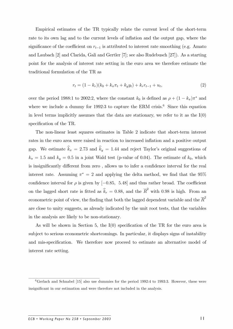
rate to its own lag and to the current levels of inflation and the output gap, where the
significance of the coefficient on rt−1 is attributed to interest rate smoothing (e.g. Amato
and Laubach [2] and Clarida, Gali and Gertler [7]; see also Rudebusch [27]). As a starting
point for the analysis of interest rate setting in the euro area we therefore estimate the
traditional formulation of the TR as
rt = (1− kr)(k0 + kππt + kyyt) + krrt−1 + ut, (2)
over the period 1988:1 to 2002:2, where the constant k0 is defined as ρ+ (1− kπ)π∗ andwhere we include a dummy for 1992:3 to capture the ERM crisis.6 Since this equation
in level terms implicitly assumes that the data are stationary, we refer to it as the I(0)
specification of the TR.
The non-linear least squares estimates in Table 2 indicate that short-term interest
rates in the euro area were raised in reaction to increased inflation and a positive output
gap. We estimate bkπ = 2.73 and bky = 1.44 and reject Taylor’s original suggestions of
kπ = 1.5 and ky = 0.5 in a joint Wald test (p-value of 0.04). The estimate of k0, which
is insignificantly different from zero , allows us to infer a confidence interval for the real
interest rate. Assuming π∗ = 2 and applying the delta method, we find that the 95%
confidence interval for ρ is given by [−0.85, 5.48] and thus rather broad. The coefficienton the lagged short rate is fitted as bkr = 0.88, and the R
2with 0.98 is high. From an
econometric point of view, the finding that both the lagged dependent variable and the R2
are close to unity suggests, as already indicated by the unit root tests, that the variables
in the analysis are likely to be non-stationary.
As will be shown in Section 5, the I(0) specification of the TR for the euro area is
subject to serious econometric shortcomings. In particular, it displays signs of instability
and mis-specification. We therefore now proceed to estimate an alternative model of
interest rate setting.
6Gerlach and Schnabel [15] also use dummies for the period 1992:4 to 1993:3. However, these were
insignificant in our estimation and were therefore not included in the analysis.
Empirical estimates of the TR typically relate the current level of the short-term
ECB • Work ing Pape r No 258 • Sep tember 2003 11

Table 2: The traditional I(0) specification of the TR
rt = (1− kr)(k0 + kππt + kyyt) + krrt−1 + et
k0-1.228
(1.593)
kπ2.733∗∗∗
(0.546)
ky1.443∗
(0.759)
kr0.884∗∗∗
(0.043)
R2
0.976
Note: Non-linear least squares estimates, sample period 1988:1-2002:2. Dummy for 1992:3
included but not reported here, standard errors in parentheses (), ∗/∗∗/∗∗∗ denotes significanceat the ten / five / one percent level.
4 A cointegration approach to the Taylor rule
We next present a formulation of the TR which takes the non-stationarity of the data
into account and which thereby captures the dynamics of the interest rates, inflation and
the output gap better.7 As a first step, we test for the number of cointegrating vectors in
the data.
4.1 The number of cointegrating vectors
In order to assess the number n of cointegrating vectors linking the short and long-term
interest rates, inflation and the output gap, we perform Johansen cointegration tests
on a system with a lag length of four.8 Table 3 shows the trace and the maximum
7In related work (Gerlach-Kristen [16]), an I(1) specification of the TR results from a
general-to-specific modelling strategy.8We started out with a model of six lags and then reduced the number of lags one by one using F-tests
to assess the validity of the restrictions. The first test to reject was that comparing a system of four lags
to one of three.
ECB • Work ing Pape r No 258 • Sep tember 200312

eigenvalue statistics for the hypotheses that n = 0 and n ≤ 1 to 3. Using the large samplecritical values, we reject the hypothesis of no cointegrating relationship, but accept that
of n ≤ 1.9 ,10 This indicates that there appears to be only one level relationship betweenrt, lt, πt and yt, which we interpret below as an interest rate reaction function.
Table 3: Johansen tests for the number of cointegrating vectors
trace statistics max. eigenvalue statistics
test statistics
(small sample)
95% critical
value
test statistics
(small sample)
95% critical
value
n = 029.8∗∗
(20.1)27.1
49.8∗∗
(35.0)47.2
n ≤ 1 13.3
(9.4)21.0
20.0
(14.0)29.7
n ≤ 2 6.0
(4.2)14.1
6.7
(4.7)15.4
n ≤ 3 0.6
(0.4)3.8
0.6
(0.5)3.8
Note: Johansen tests for n cointegrating vectors, 1989:1 - 2002:2. ∗∗ denotes significance at thefive percent level.
It is worth noting that the discussion in Section 6 implies that we would expect a
second cointegrating vector which links the long interest rate and long-run inflation. Our
failure to find evidence of this second cointegrating relationship, however, may not be
surprising given the short sample period. Johansen tests rely on asymptotics, which
implies that the test results in Table 3 should not be over-interpreted.
4.2 Estimating the cointegrating vector
Usually, the next step in the analysis would be to estimate the full vector error-correction
model. This system would in our case consist of four equations, each describing the
9As usual in the literature we also report the small sample test statistics, even though the merits of
this correction are unclear (see Doornik and Hendry [11]).10Johansen tests including only rt, πt and yt detect no evidence of any cointegrating vector. It thus
appears that the long rate plays a crucial role in the analysis.
ECB • Work ing Pape r No 258 • Sep tember 2003 13

reaction of ∆rt, ∆lt, ∆πt and ∆yt, respectively, to deviations from the cointegrating
relationship. However, the number of parameters to be fitted under this approach is
too large given the short data sample. In particular, if we were to estimate a vector
error-correction model with four lags, we would be required to estimate 75 coefficients on
58 data points.11 We therefore instead follow the single-equation approach discussed by
Hamilton [18] to estimate the cointegrating vector. This approach allows us to focus on
one variable, which in our case is the short-term interest rate, and thereby reduces the
number of parameters to be estimated drastically. Moreover, and in contrast to standard
OLS based estimates of the cointegrating vector, this technique does not require the
right-hand side variables to be weakly exogenous.
The cointegrating vector is given by
r = bll + bππ + byy, (3)
where the normalisation has been chosen such that the coefficient on the short-term
interest rate is unity. Note that equation (3) coincides with the original TR if bl = 0,
bπ = 1.5 and by = 0.5.
Since any of the four variables might adjust to disequilibria in the cointegrating vector,
a correction for the potential endogeneity bias which arises in the estimation of bl, bπ and
by is necessary.12 Hamilton suggests estimating equation (3) by including the current,
past and future changes of the right-hand side variables. We then fit
rt = a+ bllt + bππt + byyt +1X
p=−1(alp∆lt+p + aπp∆πt+p + ayp∆yt+p) + vt. (4)
Hamilton argues that the residuals vt are likely to be serially correlated and proposes
applying a GLS technique originally due to Stock and Watson [29] to correct the standard
errors. We assume an AR(1) structure for vt to arrive at the estimates presented in Table
4.13 For brevity, we only present the estimates of the b coefficients and not of the auxiliary
11Of these parameters, four are constants, 64 describe the reaction of ∆rt, ∆lt, ∆πt and ∆yt to their
lagged values, three capture the cointegrating vector and another four are the feedback coefficients.12See Maddala and Kim [24] for alternative approaches to correct this bias.13Estimations assuming an AR(2) process for vt lead to very similar results. We set p = −1 to 1
since preliminary estimations with two lags and leads yielded insignificant coefficient estimates for the
variables with p = −2 and 2.
a parameters.
ECB • Work ing Pape r No 258 • Sep tember 200314

Table 4: Estimation of the cointegrating vector
rt = a+ bllt + bππt + byyt +P1
p=−1 (alp∆lt+p + aπp∆πt+p + ayp∆yt+p) + vt
and
ρt = ea+ebllt +ebyyt +P1p=−1 (ealp∆lt+p + eayp∆yt+p) + evt
equation (4) equation (5)
bl0.827∗∗∗
(0.174)ebl 0.771∗∗∗
(0.146)
bπ0.900∗∗
(0.365)ebπ 1.000
(restricted)
by0.358∗
(0.207)eby 0.437∗∗
(0.209)
R2
0.648 R2
0.460
Note: GLS estimates, sample 1988:3-2002:1. Standard errors in parentheses (), ∗/∗∗/∗∗∗
denotes significance at the ten / five / one percent level. Estimates of auxiliary coefficients a
and ea not reported.Interestingly, the coefficient estimate on the output gap is with 0.36 close to the value
of 0.5 originally suggested by Taylor, while the sum of the parameters fitted for lt and πt
(0.83 + 0.90 = 1.73) is close to the coefficient of 1.5 proposed for inflation. We define the
error-correction term as ecrt = rt−0.83lt− 0.90πt− 0.36yt and will use it in Section 4.4 toassess how ∆rt adapts to disequilibria. First, however, we study the cointegrating vector
more carefully.
4.3 Interpreting the cointegrating vector
In the estimation of equation (3) we obtain coefficients on the inflation rate and the output
gap which are close to those originally suggested by Taylor. A Wald test does not reject
Hypothesis 1 : bπ = 1.5, by = 0.5
ECB • Work ing Pape r No 258 • Sep tember 2003 15

and yields a p-value of 0.20 (see Table 5). However, interpreting the cointegrating vector
as the original TR would imply ignoring the role of the long-term interest rate.
Table 5: Hypothesis tests for the cointegrating vector
r = bll + bππ + byy
Hypothesis p-value
1: bπ = 1.5, by = 0.5 0.198
2: bπ = 1.0 0.785
3: bπ = 1, bl = by = 0.5 0.164
Note: Coefficient on rt is normalised to unity.
We argue in Section 6 that movements in lt capture shifts in the public’s perception of
the long-run inflation objective. If this is the case, equation (3) represents a forward-looking
version of the TR since the short-term rate tends to be raised in reaction to expected
future long-run inflation. It seems natural to ask why both the current rate of inflation
and the public’s long-run expectation of it should enter the reaction function. One possible
explanation is that policymakers set rt such that the real short-term nominal interest rate
responds to long-run inflation expectations and the output gap. We therefore next test
whether πt can be restricted to have a unit coefficient in the cointegrating vector, i.e.
whether
Hypothesis 2 : bπ = 1.0,
and obtain a p-value of 0.78. This results leads us to consider as restricted I(1) specification
of the TR the model for which the error-correction term is obtained from
ρt = ea+ebllt +ebyyt + 1Xp=−1
(ealp∆lt+p + eayp∆yt+p) + evt. (5)
The second column of Table 4 shows that ebl is somewhat smaller than bl in equation (4)and that eby is larger than by.14 We define the error-correction term resulting from this
specification of the TR as ecρt = ρt − 0.77lt − 0.44yt.
14However, a test of the joint hypothesis ebl = bl and eby = by does not reject (p-value of 0.89).
ECB • Work ing Pape r No 258 • Sep tember 200316
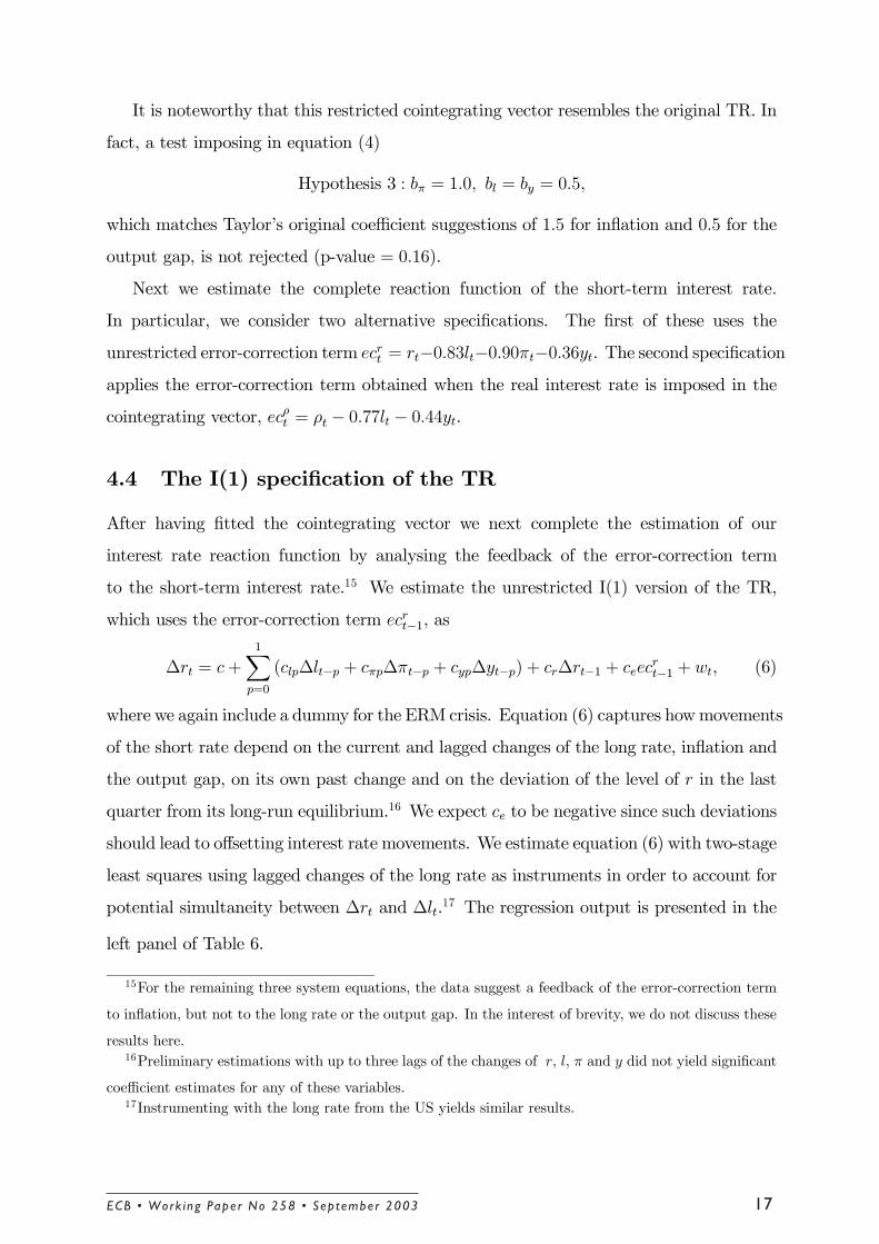
It is noteworthy that this restricted cointegrating vector resembles the original TR. In
fact, a test imposing in equation (4)
Hypothesis 3 : bπ = 1.0, bl = by = 0.5,
which matches Taylor’s original coefficient suggestions of 1.5 for inflation and 0.5 for the
output gap, is not rejected (p-value = 0.16).
Next we estimate the complete reaction function of the short-term interest rate.
In particular, we consider two alternative specifications. The first of these uses the
unrestricted error-correction term ecrt = rt−0.83lt−0.90πt−0.36yt. The second specificationapplies the error-correction term obtained when the real interest rate is imposed in the
cointegrating vector, ecρt = ρt − 0.77lt − 0.44yt.
4.4 The I(1) specification of the TR
After having fitted the cointegrating vector we next complete the estimation of our
interest rate reaction function by analysing the feedback of the error-correction term
to the short-term interest rate.15 We estimate the unrestricted I(1) version of the TR,
which uses the error-correction term ecrt−1, as
∆rt = c+1Xp=0
(clp∆lt−p + cπp∆πt−p + cyp∆yt−p) + cr∆rt−1 + ceecrt−1 + wt, (6)
where we again include a dummy for the ERM crisis. Equation (6) captures howmovements
of the short rate depend on the current and lagged changes of the long rate, inflation and
the output gap, on its own past change and on the deviation of the level of r in the last
quarter from its long-run equilibrium.16 We expect ce to be negative since such deviations
should lead to offsetting interest rate movements. We estimate equation (6) with two-stage
least squares using lagged changes of the long rate as instruments in order to account for
potential simultaneity between ∆rt and ∆lt.17 The regression output is presented in the
15For the remaining three system equations, the data suggest a feedback of the error-correction term
to inflation, but not to the long rate or the output gap. In the interest of brevity, we do not discuss these
results here.16Preliminary estimations with up to three lags of the changes of r, l, π and y did not yield significant
coefficient estimates for any of these variables.17Instrumenting with the long rate from the US yields similar results.
left panel of Table 6.
ECB • Work ing Pape r No 258 • Sep tember 2003 17

The restricted I(1) specification of the TR, which uses ecρt−1 instead of ecrt−1, is given
by
∆rt = ec+ 1Xp=0
(eclp∆lt−p + ecπp∆πt−p + ecyp∆yt−p) + ecr∆rt−1 + eceecρt−1 + wt. (7)
The regression results are shown in the right panel of the table. Next we drop insignificant
variables and obtain the final specifications
∆rt = c+ cπ0∆πt + cy0∆yt + cr∆rt−1 + ceecrt−1 + wt (8)
and
∆rt = ec+ ecπ0∆πt + ecy0∆yt + ecr∆rt−1 + eceecρt−1 + wt, (9)
the regression output for which also is reported in Table 6. The constants in equations
(8) and (9) are negative, which suggests that interest rates in the euro area tended to
decline between 1988 and 2002. This might capture the convergence of European interest
rates. Furthermore, changes in the interest rate seem to be autocorrelated and to react
to movements of inflation and the output gap as well as to the error-correction term.
As expected, a deviation of the level of the short-term interest rate from its long-run
equilibrium appears to cause offsetting future interest rate changes.
It is notable that the current change of the long rate does not seem to impact on
∆rt. However, this is compatible with the interpretation of lt as a proxy for the market
perception of the long-run inflation objective. As we show in Section 6, a better measure of
this perception, which is available only for a short sample period, is effectively uncorrelated
with changes in the short-term rate.
Lastly, Table 6 indicates that the restricted I(1) specification of the TR, which explores
the possibility that short-term interest rates respond to the real rate and which therefore
uses ecρt , fits the data virtually as well as its unrestricted counterpart, which applies
ecrt . Having estimated two versions of the TR using the cointegration approach, we next
demonstrate that these I(1) specifications capture the interest rate setting in the euro
area better than the traditional model.
ECB • Work ing Pape r No 258 • Sep tember 200318

Table 6: Cointegration specification of the TR
unrestricted I(1) restricted I(1)
equation (6) equation (8) equation (7) equation (9)
TSLS OLS TSLS OLS
c-0.377∗∗∗
(0.105)
-0.418∗∗∗
(0.104)ec -0.342∗∗∗
(0.098)
-0.378∗∗∗
(0.096)
cl00.362
(0.615)- ecl0 0.335
(0.602)-
cl1-0.066
(0.373)- ecl1 -0.043
(0.363)-
cπ00.473
(0.311)
0.628∗∗∗
(0.151)ecπ0 0.486
(0.307)
0.629∗∗∗
(0.151)
cπ10.192
(0.163)- ecπ1 0.187
(0.162)-
cy00.190∗
(0.110)
0.266∗∗∗
(0.089)ecy0 0.203∗
(0.109)
0.278∗∗∗
(0.089)
cy1-0.029
(0.106)- ecy1 -0.030
(0.106)-
cr0.351∗∗
(0.139)
0.370∗∗∗
(0.091)ecr 0.339∗∗
(0.136)
0.361∗∗∗
(0.091)
ce-0.171∗∗∗
(0.051)
-0.189∗∗∗
(0.049)ece -0.165∗∗∗
(0.048)
-0.183∗∗∗
(0.048)
R2
0.617 0.578 R2
0.619 0.576
AIC - 0.755 AIC - 0.758
BIC - 0.972 BIC - 0.975
Note: TSLS and OLS estimates, sample 1988:4-2002:2 and 1988:3-2002:2, respectively.
Instruments are lagged changes of the long rate. Standard errors in parentheses (), ∗/∗∗/∗∗∗
denotes significance at the ten / five / one percent level, AIC the Akaike criterion, BIC the
Schwarz criterion. Dummy for 1992:3 included but not reported here.
ECB • Work ing Pape r No 258 • Sep tember 2003 19

5 Comparison of the models
Section 3 argued that the non-stationarity of interest rates, inflation and the output gap
in the euro area might invalidate the conclusions drawn from the traditionally specified
TR. We here present evidence of the econometric shortcomings of this model and compare
it to the two I(1) specifications derived in Section 4. First, we present the results from
a series of diagnostic tests. Second, we simulate the three versions of the TR in order to
assess the responsiveness of the short-term interest rate to permanent shocks in inflation
and the output gap. Third, we discuss the forecasting ability of the different reaction
functions.
5.1 Diagnostic tests
Table 7 presents the test statistics for a number of standard diagnostic tests. Note that,
while the residuals of the traditional I(0) formulation appear autocorrelated, both I(1)
specifications pass tests for serial correlation in the residuals. This suggests that the
traditionally specified TR fails to capture appropriately the dynamics of the data. We do
not detect evidence of non-normality, ARCH, heteroskedasticity or model mis-specification,
as defined in the reset test, for any of the three models.
Next we turn to the stability of the different models. Given that they are estimated
over a sample which includes the convergence of the national economies before the intro-
duction of the euro, one might expect parameter instability. Figure 2 presents the cusum
and cusum of squares for the three models. While we detect signs of instability for the
traditional specification of the TR, the I(1) models perform well.18
In order to test for structural breaks, we recursively calculate Chow breakpoint tests.
Figure 3 shows that the test statistics for the I(1) specifications of the TR lie above the
ten percent critical value and thus reveal no evidence of a structural break. Interestingly,
there also is no sign of instability in 1999. The introduction of the euro thus does not
seem to have altered interest rate setting significantly.19 For the I(0) formulation, on the
18Recursive coefficient estimates appear stable for all three specifications and are not reported for
brevity.19It could thus be argued that shifting the responsibility for monetary policy to the ECB did not
ECB • Work ing Pape r No 258 • Sep tember 200320

Figure 2: Cusum tests
Cumulated sum of residuals Cumulated sum of squared residuals
traditional I(0)
-40
-30
-20
-10
0
10
20
93 94 95 96 97 98 99 00 01-0.4
0.0
0.4
0.8
1.2
1.6
93 94 95 96 97 98 99 00 01
unrestricted I(1)
-20
-10
0
10
20
93 94 95 96 97 98 99 00 01-0.4
0.0
0.4
0.8
1.2
1.6
93 94 95 96 97 98 99 00 01
restricted I(1)
-20
-10
0
10
20
93 94 95 96 97 98 99 00 01-0.4
0.0
0.4
0.8
1.2
1.6
93 94 95 96 97 98 99 00 01
Note: Cumulated sums of simple and squared residuals with 95% confidence intervals.
ECB • Work ing Pape r No 258 • Sep tember 2003 21

Table 7: F-test statistics of diagnostic tests
Specification of TR
Hypothesis
(test)traditional I(0) unrestricted I(1) restricted I(1)
No AR(1)
(Q-statistics)14.657∗∗ 0.001 0.001
Normality
(Jarque-Bera test)1.297 0.015 0.038
No serial correlation
(F-statistics LM(2))9.334∗∗∗ 0.001 0.002
No ARCH
(F-statistics LM(1))1.726 0.113 0.100
No heteroskedasticity
(F-statistics White test)1.141 0.484 0.557
No mis-specification
(F-statistics reset(1))0.629 1.646 1.880
Note: Sample period for traditional I(0) specification of the TR 1988:2 - 2002:2, for the I(1)
formulations 1988:3 - 2002:2. ∗/∗∗/∗∗∗ denotes significance at the ten / five / one percent level.
other hand, the Chow tests indicate instability. It thus appears that the traditional model
is not stable over the sample period, which suggests that it might forecast poorly.
Overall, these results point to considerable econometric shortcomings of the standard
formulation of the TR. It seems preferable to model interest rate setting in the euro
area using the cointegration approach instead. However, and as mentioned above, the
non-stationarity of the data and the problems arising in the estimation of the I(0) model
may disappear as more observations for the euro area become available.
5.2 Simulations
Next we present the simulated reactions of the short-term interest rate to a permanent
increase in inflation and the output gap, respectively. The purpose of this analysis is to
compare the dynamics implied by the three specifications of the TR. In particular, we
expose interest rate setting in the euro area to the Lucas critique (Lucas [23]).
ECB • Work ing Pape r No 258 • Sep tember 200322

Figure 3: p-values of recursive Chow tests
.0
.1
.2
.3
.4
.5
.6
.7
1994 1995 1996 1997 1998 1999 2000
traditional I(0)unrestricted I(1)restricted I(1)
Note: p-values of recursive estimates of Chow breakpoint tests with 10% critical value.
examine whether the size and speed of interest rate responses are similar for all models
or whether they suggest different degrees of responsiveness of monetary policy.
Figure 4 shows the interest rate reaction to a permanent unit increase in t = 1 of
inflation (upper plot) and of the output gap (lower plot). The policy response under the
traditional specification of the TR implies both for the inflation and the output gap shock
a small immediate increase of the interest rate that is subsequently slowly undone. The
I(1) formulations, by contrast, predict a large immediate response of the interest rate and
a fast return to equilibrium.
The sharp differences in the estimated dynamic responses provide additional evidence
that the traditional specification of the TR fails to capture fully the dynamics in the data.
Moreover, they imply that if past patterns of interest rate setting are used to understand
policy decisions by the ECB, it is important that the non-stationarity of the data be taken
into account. In particular, assume that policy decisions are best described by the I(1)
specification but that the researcher instead uses the traditional TR to forecast interest
ECB • Work ing Pape r No 258 • Sep tember 2003 23

rate changes. In this situation, actual monetary policy is likely to be more activist than
predicted by his model.
Figure 4: Simulated responses of the short-term interest rate
-0.2
0.0
0.2
0.4
0.6
0.8
1.0
2 4 6 8 10 12 14 16 18 20
traditional I(0)unrestricted I(1)restricted I(1)
Reaction to a shock in inflation
-.1
.0
.1
.2
.3
.4
.5
.6
2 4 6 8 10 12 14 16 18 20
traditional I(0)unrestricted I(1)restricted I(1)
Reaction to a shock in the output gap
Note: Responses to a permanent unit increase of inflation at time t = 1 (upper plot)
and of the output gap (lower plot).
ECB • Work ing Pape r No 258 • Sep tember 200324

5.3 Forecasts
As an alternative test for mis-specification we compare the forecasts of the three models.
For this purpose, we re-estimate the three reaction functions up to 1998:4 and use the
remaining observations to evaluate the out-of-sample forecasts. Choosing 1998:4 as end
point of the sample allows us to test whether reaction functions estimated with data up
to the introduction of the euro are able to capture the interest rate setting of the ECB.
Figure 5 shows the static and dynamic forecasts of rt for 1999:1 to 2002:2. The static
forecast calculates the predicted short-term interest rate at time t using the actual lagged
short-term rate, while the dynamic forecast uses past forecasts of rt. Note that we always
use the actual values of lt, πt and yt.
For the I(0) formulation of the TR the actual interest rate lies within the 95% confidence
band of the static forecast, but deviates significantly from the dynamic forecast from 2001
onwards. This casts doubt on the forecasting ability of the traditional specification of
the TR. The same conclusion is reached for the unrestricted I(1) model, the forecasts of
which resemble those of the I(0) specification. By contrast, the restricted I(1) formulation
appears to predict actual policy well. The short-term interest rate lies outside the 95%
confidence interval of the static forecast only once, and it stays within the confidence
region of the dynamic prediction for the entire forecast period. Thus, this specification of
the TR seems to reflect interest rate setting before and after the introduction of the euro
well.
Table 8 shows the root mean squared errors of the different forecasts. The restricted
cointegration model yields the smallest errors for both the static and the dynamic method,
while the traditional I(0) formulation of the TR displays the worst performance in the
static and the unrestricted I(1) specification in the dynamic forecast. Conditional on the
caveat that the non-stationarity of the data series studied here might disappear in the
years to come, it appears that the restricted I(1) model of the TR describes interest rate
setting in the euro area best.
ECB • Work ing Pape r No 258 • Sep tember 2003 25

Figure 5: Interest rate forecasts (in percent)
One-step-ahead static forecast s One-step-ahead dynamic forecasts
traditional I(0)
1
2
3
4
5
6
7
99 00 01 021
2
3
4
5
6
7
8
9
99 00 01 02
unrestricted I(1)
1
2
3
4
5
6
7
99 00 01 021
2
3
4
5
6
7
8
9
10
99 00 01 02
restricted I(1)
1
2
3
4
5
6
7
99 00 01 021
2
3
4
5
6
7
8
9
99 00 01 02
Note: Static and dynamic out-of-sample forecasts. Solid lines show the actual interest rate.
ECB • Work ing Pape r No 258 • Sep tember 200326

Table 8: Root mean squared errors
Specification of the TR static forecast dynamic forecast
traditional I(0) 0.585 1.745
unrestricted I(1) 0.411 1.970
restricted I(1) 0.357 0.841
Note: RMSEs of the static and the dynamic forecasts over the period 1999:1 to 2002:2.
6 Interpreting the long rate
The analysis above rested on the assumption that the long rate is a good proxy for the
public’s perception of long-run inflation. However, this interpretation may be disputed
since the expectations hypothesis (EH) holds that lt is determined by current and expected
future short-term rates and, potentially, a constant term premium.20 Thus, movements
in long interest rates may be largely due to changes in market participants’ expectations
of monetary policy in the near term. Here we provide evidence suggesting that the long
rate does in fact also contain information on long-run inflation expectations and that, if
anything, the impact of near-term expectations on monetary policy is limited.
As a preliminary it is useful to note that the EH is typically rejected by the data,
especially when the hypothesis that the slope of the yield curve predicts future changes
in long rates is tested (see e.g. Hardouvelis [19]).21 While it often is assumed that
time-varying term premia account for this finding, Kozicki and Tinsley [20] and [21]
argue that the EH is rejected because the long rate is critically influenced also by market
participants’ expectations for the short rate in the distant future, which are related to
their perceptions of policymakers’ long-run inflation objective. Hence, shifts in market
participants’ views of the long-run inflation rate (or of the credibility of monetary policy)
may be an important determinant of lt.
Kozicki and Tinsley operationalise this concept by defining an ”endpoint” of the
short-term rate process. This endpoint, which they denote as r(t)∞ (we follow their notation
20Cochrane [9] contains an excellent overview of the EH.21Regressing the change in the long rate on the spread between the long and the short rate (using
compounded rates) yields an insignificant parameter estimate also for the euro area.
ECB • Work ing Pape r No 258 • Sep tember 2003 27

below), need not be closely correlated with the current stance of monetary policy, and is
constructed from the observed term structure as
r(t)∞ =DT lT,t −Dτ lτ ,tDT −Dτ
, (10)
where D denotes the duration and where T and τ are the maturities of two underlying
long-run investments (T > τ).22 It should be noted that r(t)∞ is identical to the implied
forward rate between t + τ and t + T obtained from the coupon-bearing term structure
(see Campbell, Lo and MacKinley [6] p. 408, equation (10.1.20)). Goodfriend [17] argues
that movements of the long end of the term structure, which impact on this forward rate,
are useful in diagnosing ”inflation scares”, implying that policymakers may wish to react
to lt.
Kozicki and Tinsley [20] link r(t)∞ and the market expectation of long-run inflation
using the Fisher equation. They denote the public’s perception of the long-run inflation
objective as π(t)∞ and argue that the endpoint of the short rate process is given by
r(t)∞ = ρ(t)∞ + π(t)∞ ,
where ρ(t)∞ is the endpoint of the short-term real interest rate. Assuming, as in the quote
above, that ρ(t)∞ is constant, it follows that movements in π(t)∞ are directly reflected in r(t)∞ .
We therefore construct π(t)∞ for the euro area with T = ten years and τ = seven years.23
Since the seven-year bond yield for the euro area is available from 1994:1 onwards, we
only have data on π(t)∞ for the period 1994:1 to 2002:2.
We first investigate the correlations between the changes of lt, π(t)∞ and rt and then
present regressions involving lt and π(t)∞ .24 Reporting correlations of first-differenced data,
Table 9 shows that the long rate is correlated both with the short rate and the expected
level of long-run inflation. This indicates that the use of lt as a measure of long-run
inflation may be correct, but also that it is contaminated by the current short rate. By
contrast, π(t)∞ is essentially uncorrelated with rt. We thus reach two important conclusions.
22DT is given by (1−BT )/(1−B) with B ≡ 1/(1 + lT,t).23We calculate r(t)∞ using equation (10) and set π(t)∞ equal to this variable. Given the assumption of a
constant ρ(t)∞ this does not distort the estimates of the parameter on π(t)∞ below.
24We concentrate on changes since all variables appear non-stationary (see Table 1).
ECB • Work ing Pape r No 258 • Sep tember 200328

First, movements in the long rate seem due to two factors, π(t)∞ and rt. Second, the changes
in π(t)∞ and rt appear orthogonal. Thus, there seem to be two distinct sources of movements
in the long rate.
Table 9: Correlations
∆lt ∆π(t)∞
∆π(t)∞ 0.378 1
∆rt 0.215 0.113
Note: Sample period 1994:1-2002:2.
We can test the hypothesis that lt is significant in the cointegrating vector because of
π(t)∞ by replacing the long rate with the endpoint of inflation in equation (4). Due to the
short data sample, we exclude insignificant led and lagged changes from equation (4) and
estimate
rt = a+ b0∞π
(t)∞ + b
0ππt + b
0yyt + a
0∞∆π(t)∞ + a
0π∆πt + a
0y∆yt + v
0t. (11)
For comparison, we also fit
rt = a+ bllt + bππt + byyt + al∆lt + aπ∆πt + ay∆yt + vt. (12)
Table 10 shows the regression output.25 We find that the estimate of b0∞ is smaller than
bl, which seems due to the fact that π(t)∞ is more volatile than lt (the standard deviations
are 3.24 and 1.56, respectively). While therefore R2is smaller for equation (11) as well,
long-run inflation is clearly significant in the cointegrating vector. A further interesting
result is that, while the estimate of b0y is roughly the same as in equation (12), b0π is larger
and has a smaller p-value than bπ. This might be due to multicollinearity between lt and
πt. Those two variables have a correlation of 0.28, while the correlation between π(t)∞ and
πt is -0.04. Using π(t)∞ instead of lt might allow for a more precise identification of the role
of current inflation in the TR. It is striking that we do not reject that b0π equals unity,
which can be interpreted as support for the restricted I(1) model.
Finally, it ought to be noted that the significance of the long rate in this study arguably
depends on the choice of sample period. Monetary policy ought to react to movements25We drop insignificant current changes in order to improve the fit of the remaining parameters.
ECB • Work ing Pape r No 258 • Sep tember 2003 29

Table 10: Sensitivity analysis of the long rate
rt = a+ b0∞π
(t)∞ + b0ππt + b
0yyt + a
0∞∆π
(t)∞ + a0π∆πt + a
0y∆yt + v
0t
and
rt = a+ bllt + bππt + byyt + al∆lt + aπ∆πt + ay∆yt + vt
equation (11) equation (12)
b0∞0.105∗∗
(0.043)bl
0.570∗∗∗
(0.097)
b0π0.760∗∗∗
(0.225)bπ
0.502∗∗
(0.207)
b0y0.230∗
(0.117)by
0.134
(0.117)
R2
0.304 R2
0.775
Note: GLS estimates, sample 1994:1-2002:2. Standard errors in parentheses (), ∗/∗∗/∗∗∗
denotes significance at the ten / five / one percent level. Equation (11) is estimated without
a0∞ and a0y, for equation (12) we drop all current changes.
in the long rate only if they reflect movements in π(t)∞ . If the ECB successfully stabilises
the public’s perception of the long-run inflation objective, the long rate should cease to
be significant in the TR for the euro area.
7 Conclusions
In this paper we compare the traditional formulation of the Taylor rule, which is estimated
on level data, to an interest rate reaction function which takes into account the non-
stationarity of the data. We show that for the euro area the traditional model displays
signs of instability and mis-specification. We estimate the Taylor rule using a cointegration
approach and demonstrate that, by contrast, this yields a stable reaction function. The
cointegrating vector of this unrestricted I(1) model comprises the nominal short and
long-term interest rates, inflation and the output gap. We demonstrate that the long
rate can be seen as a proxy for the public’s perception of long-run inflation, which implies
that interest rate setting in the euro area has in that sense been forward-looking.
ECB • Work ing Pape r No 258 • Sep tember 200330

We also consider a restricted version of the I(1) model of the Taylor rule in which a unit
coefficient on inflation is imposed. Under this specification the real short-term interest
rate is raised in reaction to an increased output gap and if markets seem to expect a higher
future inflation. Thus, monetary policy is set such that the so-called Taylor principle is
met. The resulting reaction function passes the standard specification tests and yields
better out-of-sample forecasts than the traditional Taylor rule and the unrestricted I(1)
model.
ECB • Work ing Pape r No 258 • Sep tember 2003 31

References
[1] Alesina, Alberto, Olivier Blanchard, Jordi Gali, Francesco Giavazzi and Harald
Uhlig (2001), Defining a macroeconomic framework for the euro area: Monitoring
the European Central Bank (3), CEPR, London.
[2] Amato, Jeffery D. and Thomas Laubach (1999), ”The value of interest-rate
smoothing: How the private sector helps the Federal Reserve”, Federal Reserve Bank
of Kansas City Economic Review 84 (3), pp. 47-64.
[3] Begg, David, Fabio Canova, Paul De Grauwe, Antonio Fatas and Philip Lane (2002),
Surviving the slowdown: Monitoring the European Central Bank (4), CEPR, London.
[4] Brand, Claus and Nuno Cassola (2000), ”A money demand system for euro area
M3”, ECB Working Paper 39.
[5] Breuss, Fritz (2002), ”Is ECB’s monetary policy optimal already?”, mimeo, Vienna
University.
[6] Campbell, John Y., AndrewW. Lo and A. Craig MacKinlay (1997), The econometrics
of financial markets, Princeton University Press, Princeton.
[7] Clarida, Richard, Jordi Gali and Mark Gertler (1998), ”Monetary policy rules
in practice: Some international evidence”, European Economic Review 42, pp.
1033-1067.
[8] Clausen, Volker and Bernd Hayo (2002), ”Monetary policy in the euro area — Lessons
from the first years”, ZEI Working Paper B02-09.
[9] Cochrane, John H. (2001), Asset pricing, Princeton University Press, Princeton.
[10] Coenen, Günter and Volker Wieland (2000), ”A small estimated euro area model
with rational expectations and nominal rigidities”, ECB Working Paper 30.
[11] Doornik, Jurgen A. and David F. Hendry (1997), Modelling dynamic systems using
PcFiml 9.0 for Windows, International Thomson Business Press, London.
ECB • Work ing Pape r No 258 • Sep tember 200332

[12] Fagan, Gabriel, Jérôme Henry and Ricardo Mestre (2001), ”An area-wide model
(AWM) for the euro area”, ECB Working Paper 42.
[13] Faust, Jon, John H. Rogers and Jonathan H. Wright (2001), ”An empirical
comparison of Bundesbank and ECB monetary policy rules”, Board of Governors
of the Federal Reserve System International Finance Discussion Paper 705.
[14] Gerdesmeier, Dieter and Barbara Roffia (2003), ”Empirical estimates of reaction
functions for the euro area”, ECB Working Paper 206.
[15] Gerlach, Stefan and Gert Schnabel (2000), ”The Taylor rule and interest rates in the
EMU area”, Economics Letters 67, pp. 165-171.
[16] Gerlach-Kristen, Petra (2002), ”A Taylor rule for the euro area”, working paper,
University of Basel.
[17] Goodfriend, Marvin (1998), ”Using the term structure of interest rates for monetary
policy”, Federal Reserve Bank of Richmond Economic Quarterly 84 (3), pp. 13-30.
[18] Hamilton, James D. (1994), Time series analysis, Princeton University Press,
Princeton.
[19] Hardouvelis, Gikas A. (1994), ”The term structure spread and future changes in
long and short rates in the G7 countries — Is there a puzzle?”, Journal of Monetary
Economics 33, pp. 255-283.
[20] Kozicki, Sharon and P.A. Tinsley (2001), ”Shifting endpoints in the term structure
of interest rates”, Journal of Monetary Economics 47, pp. 613-652.
[21] Kozicki, Sharon and P.A. Tinsley (2001), ”Term structure views of monetary policy
under alternative models of agent expectations”, Journal of Economic Dynamics and
Control 25, pp. 149-184.
[22] Levin, Andrew, Volker Wieland and John C. Williams (1999), ”Robustness of simple
monetary policy rules and model uncertainty”; in: John B. Taylor, ed., Monetary
policy rules, Chicago University Press, Chicago.
ECB • Work ing Pape r No 258 • Sep tember 2003 33

[23] Lucas, Robert E. Jr (1976), ”Econometric policy evaluation: A critique”,
Carnegie-Rochester Conference Series on Public Policy 1, pp. 19-46.
[24] Maddala, G.S. and In-Moo Kim (2000), Unit roots, cointegration, and structural
change, Cambridge University Press, Cambridge.
[25] Orphanides, Athanasios (2000), ”The quest for prosperity without inflation”, ECB
Working Paper 15.
[26] Peersman, Gert and Frank Smets (1999), ”The Taylor rule: A useful monetary
benchmark for the euro area?”, International Finance 2 (1), pp. 85-116.
[27] Rudebusch, Glenn D. (2002), ”Term structure evidence on interest-rate smoothing
and monetary policy inertia”, Journal of Monetary Economics 49, pp. 116-1187
[28] Sack, Brian (1998), ”Uncertainty, learning, and gradual monetary policy”, Federal
Reserve Board Finance and Economics Discussion Series Paper 34.
[29] Stock, James H. and Mark W. Watson (1993), ”A simple estimator of cointegrating
vectors in higher order integrated systems”, Econometrica 61, pp. 783-820.
[30] Svensson, Lars E.O. (1999), ”Inflation targeting: Some extensions,” Scandinavian
Journal of Economics 101 (3), pp. 337-361.
[31] Taylor, John B. (1993), ”Discretion versus policy rules in practice”,
Carnegie-Rochester Conference Series on Public Policy 39, pp. 195-214.
[32] Taylor, John B. (1998), ”The robustness and efficiency of monetary policy rules as
guidelines for interest rate setting by the European Central Bank”, IIES Seminar
Paper 649.
[33] Woodford, Michael (1994), ”Nonstandard indicators for monetary policy: Can their
usefulness be judged from forecasting regressions?”, in: N. Gregory Mankiw, ed.,
Monetary policy, University of Chicago Press and NBER, Chicago.
ECB • Work ing Pape r No 258 • Sep tember 200334

European Central Bank working paper series
For a complete list of Working Papers published by the ECB, please visit the ECB’s website(http://www.ecb.int).
202 “Aggregate loans to the euro area private sector” by A. Calza, M. Manrique and J. Sousa,January 2003.
203 “Myopic loss aversion, disappointment aversion and the equity premium puzzle” byD. Fielding and L. Stracca, January 2003.
204 “Asymmetric dynamics in the correlations of global equity and bond returns” byL. Cappiello, R.F. Engle and K. Sheppard, January 2003.
205 “Real exchange rate in an inter-temporal n-country-model with incomplete markets” byB. Mercereau, January 2003.
206 “Empirical estimates of reaction functions for the euro area” by D. Gerdesmeier andB. Roffia, January 2003.
207 “A comprehensive model on the euro overnight rate” by F. R. Würtz, January 2003.
208 “Do demographic changes affect risk premiums? Evidence from international data” byA. Ang and A. Maddaloni, January 2003.
209 “A framework for collateral risk control determination” by D. Cossin, Z. Huang,D. Aunon-Nerin and F. González, January 2003.
210 “Anticipated Ramsey reforms and the uniform taxation principle: the role of internationalfinancial markets” by S. Schmitt-Grohé and M. Uribe, January 2003.
211 “Self-control and savings” by P. Michel and J.P. Vidal, January 2003.
212 “Modelling the implied probability of stock market movements” by E. Glatzer andM. Scheicher, January 2003.
213 “Aggregation and euro area Phillips curves” by S. Fabiani and J. Morgan, February 2003.
214 “On the selection of forecasting models” by A. Inoue and L. Kilian, February 2003.
215 “Budget institutions and fiscal performance in Central and Eastern European countries” byH. Gleich, February 2003.
216 “The admission of accession countries to an enlarged monetary union: a tentativeassessment” by M. Ca’Zorzi and R. A. De Santis, February 2003.
217 “The role of product market regulations in the process of structural change” by J. Messina,March 2003.
ECB • Work ing Pape r No 258 • Sep tember 2003 35

218 “The zero-interest-rate bound and the role of the exchange rate for monetary policy inJapan” by G. Coenen and V. Wieland, March 2003.
219 “Extra-euro area manufacturing import prices and exchange rate pass-through” byB. Anderton, March 2003.
220 “The allocation of competencies in an international union: a positive analysis” by M. Ruta,April 2003.
221 “Estimating risk premia in money market rates” by A. Durré, S. Evjen and R. Pilegaard,April 2003.
222 “Inflation dynamics and subjective expectations in the United States” by K. Adam andM. Padula, April 2003.
223 “Optimal monetary policy with imperfect common knowledge” by K. Adam, April 2003.
224 “The rise of the yen vis-à-vis the (“synthetic”) euro: is it supported by economicfundamentals?” by C. Osbat, R. Rüffer and B. Schnatz, April 2003.
225 “Productivity and the (“synthetic”) euro-dollar exchange rate” by C. Osbat, F. Vijselaar andB. Schnatz, April 2003.
226 “The central banker as a risk manager: quantifying and forecasting inflation risks” byL. Kilian and S. Manganelli, April 2003.
227 “Monetary policy in a low pass-through environment” by T. Monacelli, April 2003.
228 “Monetary policy shocks – a nonfundamental look at the data” by M. Klaeffing, May 2003.
229 “How does the ECB target inflation?” by P. Surico, May 2003.
230 “The euro area financial system: structure, integration and policy initiatives” byP. Hartmann, A. Maddaloni and S. Manganelli, May 2003.
231 “Price stability and monetary policy effectiveness when nominal interest rates are boundedat zero” by G. Coenen, A. Orphanides and V. Wieland, May 2003.
232 “Describing the Fed’s conduct with Taylor rules: is interest rate smoothing important?” byE. Castelnuovo, May 2003.
233 “The natural real rate of interest in the euro area” by N. Giammarioli and N. Valla,May 2003.
234 “Unemployment, hysteresis and transition” by M. León-Ledesma and P. McAdam,May 2003.
235 “Volatility of interest rates in the euro area: evidence from high frequency data” byN. Cassola and C. Morana, June 2003.
ECB • Work ing Pape r No 258 • Sep tember 200336

236 “Swiss monetary targeting 1974-1996: the role of internal policy analysis” by G. Rich, June2003.
237 “Growth expectations, capital flows and international risk sharing” by O. Castrén, M. Millerand R. Stiegert, June 2003.
238 “The impact of monetary union on trade prices” by R. Anderton, R. E. Baldwin andD. Taglioni, June 2003.
239 “Temporary shocks and unavoidable transitions to a high-unemployment regime” byW. J. Denhaan, June 2003.
240 “Monetary policy transmission in the euro area: any changes after EMU?” by I. Angeloni andM. Ehrmann, July 2003.
241 Maintaining price stability under free-floating: a fearless way out of the corner?” byC. Detken and V. Gaspar, July 2003.
242 “Public sector efficiency: an international comparison” by A. Afonso, L. Schuknecht andV. Tanzi, July 2003.
243 “Pass-through of external shocks to euro area inflation” by E. Hahn, July 2003.
244 “How does the ECB allot liquidity in its weekly main refinancing operations? A look at theempirical evidence” by S. Ejerskov, C. Martin Moss and L. Stracca, July 2003.
245 “Money and payments: a modern perspective” by C. Holthausen and C. Monnet, July 2003.
246 “Public finances and long-term growth in Europe – evidence from a panel data analysis” byD. R. de Ávila Torrijos and R. Strauch, July 2003.
247 “Forecasting euro area inflation: does aggregating forecasts by HICP component improveforecast accuracy?” by K. Hubrich, August 2003.
248 “Exchange rates and fundamentals” by C. Engel and K. D. West, August 2003.
249 “Trade advantages and specialisation dynamics in acceding countries” by A. Zaghini, August2003.
250 “Persistence, the transmission mechanism and robust monetary policy” by I. Angeloni,G. Coenen and F. Smets, August 2003.
251 “Consumption, habit persistence, imperfect information and the lifetime budget constraint” by A. Willman, August 2003.
252 “Interpolation and backdating with a large information set”, by E. Angelini, J. Henry and M. Marcellino, August 2003.
253 “Bond market inflation expectations and longer-term trends in broad monetary growthand inflation in industrial countries, 1880-2001”, by W. G. Dewald, September 2003.
ECB • Work ing Pape r No 258 • Sep tember 2003 37

254 “Forecasting real GDP: what role for narrow money?”, by C. Brand, H.-E. Reimers and F. Seitz, September 2003.
255 “Is the demand for euro area M3 stable?”, by A. Bruggeman, P. Donati and A. Warne,September 2003.
256 “Information acquisition and decision making in committees: a survey”, by K. Gerling, H. P. Grüner, A. Kiel and E. Schulte, September 2003.
ECB • Work ing Pape r No 258 • Sep tember 200338
258 “Interest rate reaction functions and the Taylor rule in the euro area”, by P. Gerlach-Kristen,September 2003.
257 “Macroeconomic modelling of monetary policy”, by M. Klaeffling, September 2003.