Eulerian-on-Lagrangian SimulationYe Fan, Joshua Litven, David I.W. Levin, and Dinesh K. PaiDepartment of Computer Science, University of British Columbia1

We describe an Eulerian-on-Lagrangian solid simulator that reduces oreliminates many of the problems experienced by fully Eulerian methodsbut retains its advantages. Our method does not require the constructionof an explicit object discretization and the fixed nature of the simulationmesh avoids tangling during large deformations. By introducing Lagrangianmodes to the simulation we enable unbounded simulation domains and re-duce the time-step restrictions which can plague Eulerian simulations. Ourmethod features a new solver that can resolve contact between multiple ob-jects while simultaneously distributing motion between the Lagrangian andEulerian modes in a least-squares fashion. Our method successfully bridgesthe gap between Lagrangian and Eulerian simulation methodologies with-out having to abandon either one.

Categories and Subject Descriptors: I.6.8 [Simulation and Modeling]:Types of Simulation

Additional Key Words and Phrases: Deformation, Continuum Mechanics,Rigid Bodies, Eulerian, Contact

1. INTRODUCTION

Eulerian simulations have proven to be indispensable tools in thecomputer graphics field. They are used to produce stunning an-imations of complicated fluids, and more recently, of solids andgranular materials. Because these simulations rely on a fixed spa-tial discretization they avoid many of the perils encountered by La-grangian simulation of highly deformable objects. However, thesemethods suffer from inherent drawbacks stemming from the fixedspatial discretization which is their defining characteristic. Chiefamongst these is the necessary discretization of the entire simula-tion domain, difficulties in computing accurate and dissipation freeadvection, and potential time-step restrictions. Many algorithms at-tempt to avoid these issues by replacing parts, or all of the sim-ulation with Lagrangian methods, but this is done at the peril oflosing the advantages of the Eulerian approach. In this paper wepresent a clean, hybrid technique which allows us to leverage thebenefits of Lagrangian and Eulerian simulators by treating rigid andlow frequency modes of a deformable object as Lagrangian and thehigh frequency deformable modes as Eulerian. We will show thatthis approach alleviates or significantly reduces all of the problemslisted above but still allows us to resolve large deformations con-veniently in an Eulerian context. We also detail a contact-awaresolver for these types of mixed Eulerian-Lagrangian simulations.See Figure 1 for a preview of the results.

2. RELATED WORK

Eulerian simulations have become commonplace in computergraphics, especially in fluids simulation. Eulerian simulations havebeen used to simulate melting solids [Carlson et al. 2002], vis-coelastic fluids [Goktekin et al. 2004; Losasso et al. 2006] and elas-tic or elasto-plastic solids [Sulsky et al. 1994; Trangenstein 1994;Miller and Colella 2001; Tran and Udaykumar 2004; Banks et al.2007; Barton and Drikakis 2010; Kamrin and Nave 2009; Levinet al. 2011; Kamrin et al. 2012]. However, Eulerian simulations suf-

fer from several inherent drawbacks such as spatio-temporal timestep limitations [Osher and Fedkiw 2002], dissipation caused bycertain advection schemes [Stam 1999] and the necessity of defin-ing a computational domain that extends throughout the simulationdomain [Foster and Metaxas 1996]. For Eulerian fluid simulationsthese shortcomings have been addressed by using more compli-cated, conservative advection schemes [Lentine et al. 2011] anddata structures [Wang et al. 2005]. An alternate approach involvesreplacing the Eulerian computational machinery with Lagrangiananalogs [Premoze et al. 2003]. However in theses cases we arefaced with losing the advantages conferred by Eulerian simulation.Methods which maintain Eulerian and Lagrangian characteristicssimultaneously can prove to be useful alternatives to these either-orapproaches. Such methods have been used effectively for simula-tion of constrained, one-dimensional strands [Sueda et al. 2011],dissipation free advection [Zhu and Bridson 2005], robust pressure-projection in particle-based fluid simulations [Narain et al. 2010;Raveendran et al. 2011] and as a means of solid fluid coupling infinite-element simulations [Belytschko and Kennedy 1978]. Ad-ditionally, methods which translate [Shah et al. 2004] or rotateand scale [Poludnenko and Khokhlov 2007] the simulation do-main have been used in fluid simulation. In this paper we will takea different approach from the methods listed above. Instead of as-signing algorithmic steps or discrete points to be Lagrangian or Eu-lerian we will imbue generalized configuration variables with thesecharacteristics via a sequence of mappings. This will allow us toassign Lagrangian and Eulerian behavior to the different modes ofa motion (not just to the nodes of a domain). We will give twospecific examples of Eulerian-on-Lagrangian methods but note thatthe algorithm described allows a completely general decompositionto be applied. As opposed to the Arbitrary-Lagrangian-Eulerianmethod [Belytschko et al. 2000] (ALE) and Lagrangian methodswhich use remeshing to avoid ill-conditioned elements [Bargteilet al. 2007; Wicke et al. 2010], our method describes a princi-pled numerical “glue” that can be used to merge Eulerian and La-grangian Simulations, both described using arbitrary generalizedcoordinates, and inherit the advantages of both schemes.

2.1 Contributions

Our main contribution is an Eulerian-on-Lagrangian simulator fordeformable elastic and elastoplastic solids, which decomposes themotion of objects using both Lagrangian and Eulerian configura-tion variables. Our second contribution is a novel solver that auto-matically resolves the inherent redundancy of this decompositionin an optimal fashion by projecting momentum onto the low di-mensional Lagrangian space while simultaneously resolving con-tact constraints acting on the system. Our third contribution is amethod for simulating plasticity without smoothing of the plasticdeformation in an Eulerian context but that avoids remeshing asis used in previous methods [Bargteil et al. 2007; Wicke et al.2010]. The presented method also features a dynamic time step-ping scheme which maximizes the time step of the Eulerian inte-grator while attempting to guarantee that the stability requirementof the Eulerian advection stage will be met in the presence of con-

ACM Transactions on Graphics, Vol. , No. , Article , Publication date: .

2 •

(a) Eulerian-on-Lagrangian Grids (b) Large Deformation (c) Plasticity (d) Multiple Objects

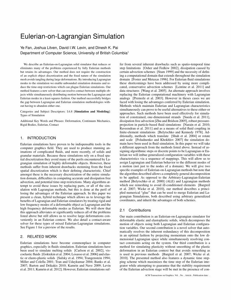
Fig. 1: (a) The Eulerian-on-Lagrangian method embeds an Eulerian solid simulator in a Lagrangian grid. (b) Elastic spheres undergo acollision with large deformations, and return to precise rest shapes. (c) Two plastic cylinders after colliding with a rigid rod. (d) Complexcontact between several Eulerian-on-Lagrangian objects.

tact. The end result is a simulator that can adaptively function as aLagrangian simulator, a fully Eulerian simulator or a combinationof the two.

3. METHODS

For the reader’s convenience we will begin by outlining the nota-tional conventions used in this paper (Table I). With a slight abuseof notation we denote both nodal variables for single elements aswell as entire objects by the same bold face letters, and the mean-ing will be evident from the context. When necessary we denotethe stacked vector of all configuration variables as q.

Table I. : Notation used

Notation Definitionf scalar or 3-vectorf n× 1 vector resulting from stacking all f•f df

dt in spatial domainf df

dt in intermediate domain[f ] cross product matrix: f×

Material(z) Intermediate(y) Spatial(x )

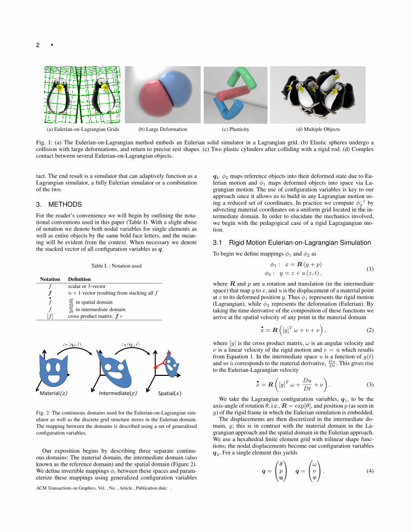
Fig. 2: The continuous domains used for the Eulerian-on-Lagrangian sim-ulator as well as the discrete grid structure stores in the Eulerian domain.The mapping between the domains is described using a set of generalizedconfiguration variables.

Our exposition begins by describing three separate continu-ous domains: The material domain, the intermediate domain (alsoknown as the reference domain) and the spatial domain (Figure 2).We define invertible mappings φi between these spaces and param-eterize these mappings using generalized configuration variables

qi. φ2 maps reference objects into their deformed state due to Eu-lerian motion and φ1 maps deformed objects into space via La-grangian motion. The use of configuration variables is key to ourapproach since it allows us to build in any Lagrangian motion us-ing a reduced set of coordinates. In practice we compute φ−1

2 byadvecting material coordinates on a uniform grid located in the in-termediate domain. In order to elucidate the mechanics involved,we begin with the pedagogical case of a rigid Lagragangian mo-tion.

3.1 Rigid Motion Eulerian-on-Lagrangian Simulation

To begin we define mappings φ1 and φ2 as

φ1 : x = R (y + p)

φ2 : y = z + u (z, t) ,(1)

where R and p are a rotation and translation (in the intermediatespace) that map y to x, and u is the displacement of a material pointat z to its deformed position y. Thus φ1 represents the rigid motion(Lagrangian), while φ2 represents the deformation (Eulerian). Bytaking the time derivative of the composition of these functions wearrive at the spatial velocity of any point in the material domain

•x = R

([y]T ω + v + ν

), (2)

where [y] is the cross product matrix, ω is an angular velocity andν is a linear velocity of the rigid motion and v = u which resultsfrom Equation 1. In the intermediate space u is a function of y(t)and so u corresponds to the material derivative, Du

Dt. This gives rise

to the Eulerian-Lagrangian velocity

•x = R

([y]T ω +

Du

Dt+ ν

). (3)

We take the Lagrangian configuration variables, q1, to be theaxis-angle of rotation θ, i.e., R = exp[θ], and position p (as seen iny) of the rigid frame in which the Eulerian simulation is embedded.

The displacements are then discretized in the intermediate do-main, y; this is in contrast with the material domain in the La-grangian approach and the spatial domain in the Eulerian approach.We use a hexahedral finite element grid with trilinear shape func-tions; the nodal displacements become our configuration variablesq2. For a single element this yields

q =

θpu

q =

ωνv

. (4)

ACM Transactions on Graphics, Vol. , No. , Article , Publication date: .

• 3

Again we note that the total time derivative of the Eulerian veloc-ity implies the application of the material derivative. In our methodthis is computed using an independant advection step (as is usuallydone in fluid mechanics, see Bridson [2008] for a good descrip-tion). Other methods bake this material derivative into the equa-tions of motion (see Sueda et al. [2011] for a depiction of such anapproach).

For the ith element we can define the Lagrangian function of oursystem as

L =1

2qTM iq − V (q) (5)

where

M i =

∫Ωi

ρJ

[y] [y]T [y] [y]N i

[y]T I N i

N iT [y]T N iT N iTN i

dΩi, (6)

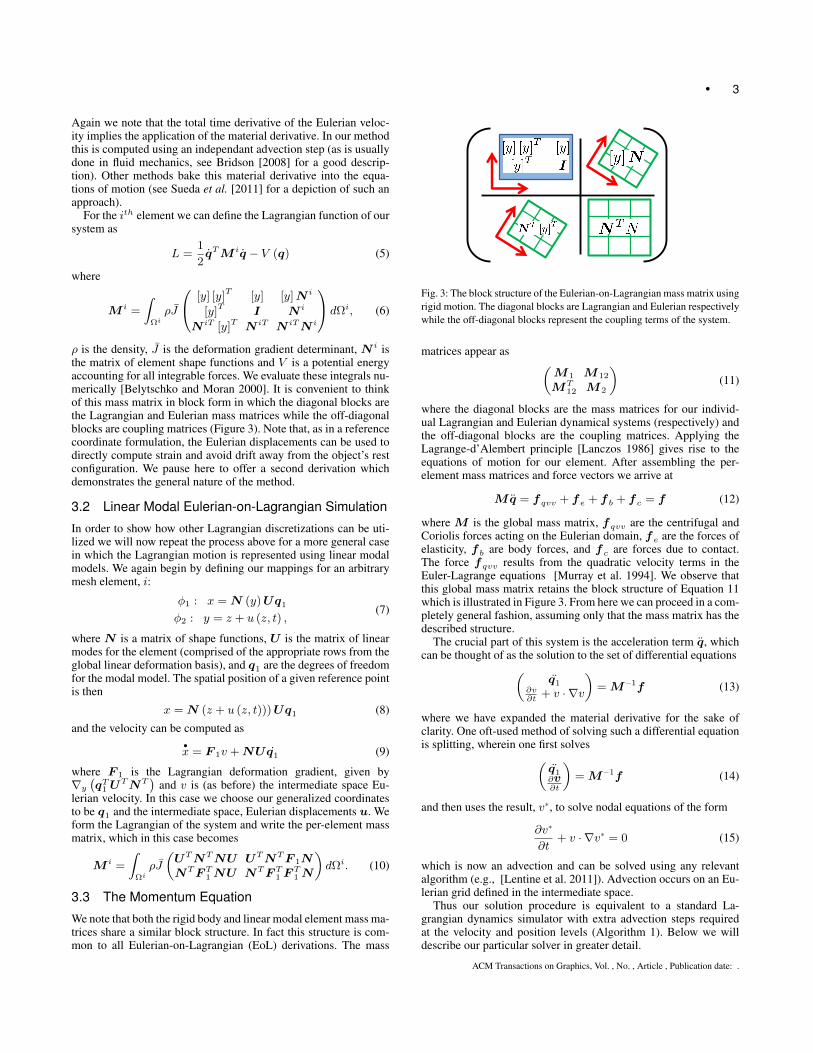
ρ is the density, J is the deformation gradient determinant, N i isthe matrix of element shape functions and V is a potential energyaccounting for all integrable forces. We evaluate these integrals nu-merically [Belytschko and Moran 2000]. It is convenient to thinkof this mass matrix in block form in which the diagonal blocks arethe Lagrangian and Eulerian mass matrices while the off-diagonalblocks are coupling matrices (Figure 3). Note that, as in a referencecoordinate formulation, the Eulerian displacements can be used todirectly compute strain and avoid drift away from the object’s restconfiguration. We pause here to offer a second derivation whichdemonstrates the general nature of the method.

3.2 Linear Modal Eulerian-on-Lagrangian Simulation

In order to show how other Lagrangian discretizations can be uti-lized we will now repeat the process above for a more general casein which the Lagrangian motion is represented using linear modalmodels. We again begin by defining our mappings for an arbitrarymesh element, i:

φ1 : x = N (y)Uq1

φ2 : y = z + u (z, t) ,(7)

where N is a matrix of shape functions, U is the matrix of linearmodes for the element (comprised of the appropriate rows from theglobal linear deformation basis), and q1 are the degrees of freedomfor the modal model. The spatial position of a given reference pointis then

x = N (z + u (z, t)))Uq1 (8)

and the velocity can be computed as•x = F 1v + NUq1 (9)

where F 1 is the Lagrangian deformation gradient, given by∇y(qT1 U

TNT)

and v is (as before) the intermediate space Eu-lerian velocity. In this case we choose our generalized coordinatesto be q1 and the intermediate space, Eulerian displacements u. Weform the Lagrangian of the system and write the per-element massmatrix, which in this case becomes

M i =

∫Ωi

ρJ

(UTNTNU UTNTF 1NNTF T

1 NU NTF T1 F

T1 N

)dΩi. (10)

3.3 The Momentum Equation

We note that both the rigid body and linear modal element mass ma-trices share a similar block structure. In fact this structure is com-mon to all Eulerian-on-Lagrangian (EoL) derivations. The mass

Fig. 3: The block structure of the Eulerian-on-Lagrangian mass matrix usingrigid motion. The diagonal blocks are Lagrangian and Eulerian respectivelywhile the off-diagonal blocks represent the coupling terms of the system.

matrices appear as (M1 M12

MT12 M2

)(11)

where the diagonal blocks are the mass matrices for our individ-ual Lagrangian and Eulerian dynamical systems (respectively) andthe off-diagonal blocks are the coupling matrices. Applying theLagrange-d’Alembert principle [Lanczos 1986] gives rise to theequations of motion for our element. After assembling the per-element mass matrices and force vectors we arrive at

Mq = fqvv + fe + f b + fc = f (12)

where M is the global mass matrix, fqvv are the centrifugal andCoriolis forces acting on the Eulerian domain, fe are the forces ofelasticity, f b are body forces, and fc are forces due to contact.The force fqvv results from the quadratic velocity terms in theEuler-Lagrange equations [Murray et al. 1994]. We observe thatthis global mass matrix retains the block structure of Equation 11which is illustrated in Figure 3. From here we can proceed in a com-pletely general fashion, assuming only that the mass matrix has thedescribed structure.

The crucial part of this system is the acceleration term q, whichcan be thought of as the solution to the set of differential equations(

q1∂v∂t

+ v · ∇v

)= M−1f (13)

where we have expanded the material derivative for the sake ofclarity. One oft-used method of solving such a differential equationis splitting, wherein one first solves(

q1∂v∂t

)= M−1f (14)

and then uses the result, v∗, to solve nodal equations of the form

∂v∗

∂t+ v · ∇v∗ = 0 (15)

which is now an advection and can be solved using any relevantalgorithm (e.g., [Lentine et al. 2011]). Advection occurs on an Eu-lerian grid defined in the intermediate space.

Thus our solution procedure is equivalent to a standard La-grangian dynamics simulator with extra advection steps requiredat the velocity and position levels (Algorithm 1). Below we willdescribe our particular solver in greater detail.

ACM Transactions on Graphics, Vol. , No. , Article , Publication date: .

4 •

Algorithm 1 A high level overview of the Eulerian-on-Lagrangiansolution procedure. Here we explicitly denote the partial timederivatives of Eulerian qualities for clarity.

1: Solve M

(q1∂v∂t

)= f for qt+1

1 and v∗

2: vt+1 = advect(v∗)

3: Solve(q1∂u∂t

)=

(q1t+1

vt+1

)for q1 and u∗

4: u = advect(u∗)

To solve step 1 of Algorithm 1, we discretize the acceleration qand solve at the velocity-impulse level, which gives

Mqt+1 = ∆tf + Mqtdef= pt+1. (16)

Using the block structure of M and suppressing the time step t+ 1for clarity,

M1q1 + M12v∗ = p1 (17a)

MT12q1 + M2v

∗ = p2, (17b)

where M1 is the nonsingular Lagrangian mass matrix, M2 is thenonsingular Eulerian mass matrix, M12 is the coupling matrix be-tween the two modes, p1 is the generalized Lagrangian momentumand p2 is the generalized Eulerian momentum(Figure 3). Becausewe lump the mass to the nodes, M2 is diagonal.

3.4 Exploiting Redundancies

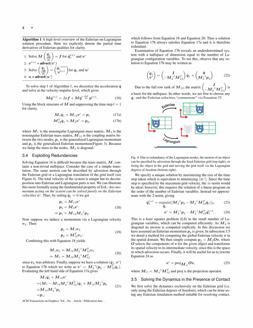
Solving Equation 16 is difficult because the mass matrix, M , con-tains a non-trivial nullspace. Consider the case of a simple trans-lation. The same motion can be described by advection throughthe Eulerian grid or a Lagrangian translation of the grid itself (seeFigure 4). The total velocity of the system is unique but its decom-position into Eulerian and Lagrangian parts is not. We can illustratethis more formally using the fundamental property of EoL: Any mo-mentum acting on the system can be solved purely on the Eulerianvelocities v∗. Thus, by setting q1 = 0 we get

p1 = M12v∗

p2 = M2v∗

⇒ p1 = M12M−12 p2.

(18)

Now suppose we induce a momentum via a Lagrangian velocityvL. Then

p1 = M1vL

p2 = MT12vL.

(19)

Combining this with Equation 18 yields

M1vL = M12M−12 MT

12vL

⇒M1 = M12M−12 MT

12

(20)

since vL was arbitrary. Finally, suppose we have a solution (q1,v∗)

to Equation 17b which we write as v∗ = M−12 (p2 −MT

12q1).Evaluating the left hand side of Equation 17a gives

M1q1 + M12v∗

=(M1 −M12M−12 MT

12)q1 + M12M−12 p2

=M12M−12 p2

=p1,

(21)

which follows from Equation 18 and Equation 20. Thus a solutionto Equation 17b always satisfies Equation 17a and it is thereforeredundant.

Examination of Equation 17b reveals an underdetermined sys-tem with a nullspace of dimension equal to the number of La-grangian configuration variables. To see this, observe that any so-lution to Equation 17b may be written as

(q1

v∗

)=

(I

−M−12 MT

12

)q1 +

(0

M−12 p2

). (22)

Due to the full row rank of M12, the matrix(

I−M−1

2 MT12

)is

a basis for the nullspace. In other words, we are free to choose anyq1 and the Eulerian velocities “compensate” via Equation 22.

Fig. 4: Due to redundancy of the Lagrangian modes, the motion of an objectcan be specified by advection through the fixed Eulerian grid (top right), orfixing the object in the grid and moving the grid itself via the Lagrangiandegrees of freedom (bottom right).

We specify a unique solution by maximizing the size of the timestep taken which is equivalent to minimizing ||v∗||. Since the timestep is specified by the maximum grid velocity, the∞-norm wouldbe ideal; however, this requires the solution of a linear program onthe order of the number of Eulerian variables. Instead we approxi-mate with the 2-norm, giving

qt+11 = argmin

q1

||M−12 p2 −M−1

2 MT12q1||2, (23)

v∗ = M−12 p2 −M−1

2 MT12q

t+11 . (24)

This is a least squares problem (LS) in the small number of La-grangian variables, which can be computed efficiently. As M2 isdiagonal its inverse is computed explicitly. In this discussion wehave assumed an Eulerian momentum p2 is given. In subsection 3.5we detail a method for computing the global Eulerian velocity v inthe spatial domain. We then simply compute p2 = M2Ov, whereO selects the components of v for the given object and transformsits spatial velocity to its intermediate velocity, since this is the spacein which advection occurs. Finally, it will be useful for us to rewriteEquation 24 as

v∗ = projMCOv, (25)

where MC = M−12 MT

12 and proj is the projection operator.

3.5 Solving the Dynamics in the Presence of Contact

We first solve the dynamics exclusively on the Eulerian grid (i.e.only using the Eulerian degrees of freedom), which can be done us-ing any Eulerian simulation method suitable for resolving contact.

ACM Transactions on Graphics, Vol. , No. , Article , Publication date: .

• 5

In our case, we invoke Gauss’ principle of least constraint [Lanczos1986], which gives the constrained optimization problem

minimize1

2aTMa− f

Ta

subject to a ∈ A,(26)

where M is a global mass matrix, a and f are the accelerations andforces defined in the spatial domain, andA is a constraint manifoldimposed on the acceleration; these constraints ensure interpenetra-tion between objects does not occur. Notice that M is assembledfrom the Eulerian mass matrices M2 in Equation 17. First orderdiscretization of the acceleration gives rise to a quadratic program(QP) on the spatial velocities with constraints we now derive. Con-sider a colliding pair of objects A and B with surfaces ΓA and ΓB ,respectively. Due to the discrete time integration there is some vol-ume of intersection Ω. We impose a velocity level constraint spec-ifying that the volume of intersection at the next time step must besmaller than Ω, giving the surface integration constraint∫

ΓA∩Ω

vA · ndΓ +

∫ΓB∩Ω

vB · ndΓ ≤ 0, (27)

where n are surface normals. Spatial velocities are representedon the Eulerian grid by trilinear shape functions. Thus expandingthe velocity terms in Equation 27 yields the constraint

n∑s=1

vAs

∫ΓA∩Ω

Φs · ndΓ + vBs

∫ΓB∩Ω

Φs · ndΓ

= jTv ≤ 0 (28)

where s indexes the nodal velocities and their associated interpo-lating functions given by Φs.

The constraints are assembled into a global constraint matrix Jand the QP solved at each time step is given by

minimize1

2vTMv − pTv

subject to Jv ≤ 0,(29)

where p is a globally assembled momentum vector. In the caseof rigid bodies with externally prescribed motion the formulationchanges slightly as the right hand side is no longer 0.

Collision detection and the computation of the surface integralsin Equation 28 require a representation of each object’s surface inthe spatial domain. Any suitable method could be used, such as thevolumetric method of [Levin et al. 2011] or recent methods basedon ray tracing [Wang et al. 2012]. In our implementation we use thereconstructed surface (see subsection 3.8), with a ray tracing colli-sion detector to produce a collection of intersection rays, barycen-tric coordinates w.r.t. the surface mesh, and normals for every pairof colliding objects. Since spatial velocities are stored in the inter-mediate domain (on the Eulerian grid), we use the barycentric co-ordinates of the intersected rays to find the corresponding positionsy and their associated degrees of freedom, from which the shapefunction values can be computed as well as the nonzero patternof J . Finally, we note that constraints between objects are decom-posed via a collision grid defined on the spatial domain to enhancethe resolution of constraints along deforming surfaces.

Equation 29 is solved via an efficient primal-dual active setmethod [Ito and Kunisch 2008]. Due to the diagonal structure of themass matrix, the complexity of the QP solver isO(m3), wherem isthe number of constraints. Once the spatial velocity v is known, we

can compute the Eulerian momentum p2 of each object. Thus step1 of Algorithm 1 amounts to a QP solve to determine the globalmomentum followed by a LS solve to optimally compute Eulerianand Lagrangian velocities. See Table II for computational runtimes.

3.6 Dynamic Time Step

Crucial to the efficiency of our approach is determining an ap-propriate time step ∆t. Here we follow the approach of [Levinet al. 2011] and extend it to the Eulerian-on-Lagrangian formula-tion. First-order advection has the stability requirement

∆t max(||v∗x||∆x

,||v∗y||∆y

,||v∗z||∆z

)≤ α (30)

for a parameter α < 1. We use a pseudo-implicit method to deter-mine ∆twhich satisfies Equation 30. One can describe the solutionto the QP Equation 29 as

v = v0 + ∆tv1, (31)

where v0 and v1 are basis vectors which can be found by solvingEquation 29 at a given time followed by a linear solve. SubstitutingEquation 31 into Equation 25 yields

v∗ = projMCO(v0 + ∆tv1) (32a)

= projMCOv0 + ∆tprojMC

Ov1 (32b)

= v∗0 + ∆tv∗1 (32c)

where v∗0 and v∗1 can be computed from v0 and v1 by solvingtwo least squares problems. Finally, we combine Equation 32c andEquation 30 to get a quadratic equation in ∆t:

γ1∆t2 + γ0∆t− α = 0, (33)

where γi =(||v∗ix||

∆x+||v∗iy ||

∆y+||v∗iz ||

∆z

). The resultant time step

is optimal in the sense that it minimizes ||v∗|| while obeying thestability criterion.

3.7 Plasticity

One advantage of Eulerian simulations is that we can avoid ma-terial, intermediate and spatial domain remeshing when simulat-ing plastic deformations. Our implementation of elastoplasticity isbased on that of Bargteil et al. [2007] and Wicke et al. [2010]. Themultiplicative plasticity model starts from the following decompo-sition of the total deformation gradient

F total = F eF p, (34)

where F e is the elastic deformation gradient and F p is the plas-tic deformation gradient. The evolution of the plastic deformationgradient is given by

(F −1p )t+1 = (F −1

p )t∆F −1p , (35)

where ∆F −1p is an update applied to F p. This update is computed

using the singular value decomposition (SVD) of the current elasticdeformation gradient:

F e = UΣV T . (36)

The plastic update is then computed as

∆F −1p = V

(Σ

(detΣ)1/3

)−γV T , (37)

ACM Transactions on Graphics, Vol. , No. , Article , Publication date: .

6 •

where γ = ν(‖σ‖−‖σy‖‖σ‖

), 0 ≤ γ ≤ 1 and ‖σy‖ is the plastic yield.

Our approach is distinguished from previous methods [Bargteilet al. 2007; Wicke et al. 2010] by the manner in which the plasticdeformation is stored. Though we allow Eulerian deformation, theavailability of a mapping to z allows us to store the plastic deforma-tion in the material domain. When computing (Equation 34) in thespatial domain, we perform a lookup for F p in z. When evolvingF p, we construct a mapping from the material domain to the spa-tial domain using local meshless interpolation methods. Using thisinterpolated displacement u, F total can be computed as I + ∂u

∂z .Subsequently, F e can be computed, followed by the SVD (Equa-tion 36). We incorporate the Lagrangian displacements into u inorder to ensure proper evolution of F p. Our approach does not re-quire remeshing, and by storing F p in the material domain, theplastic deformation gradient will not smear out during advection.

3.8 Surface Reconstruction

We leverage our Eulerian displacements to perform surface recon-struction directly from the material coordinates z. This imparts aguarantee that the surface mesh will always return to its originalshape when the simulation displacements are zero (something thatcannot be said for advecting mesh vertices in an Eulerian flow).Westore a surface mesh for our object in the material domain. Due tothe use of Lagrangian modes and adaptive time stepping, the Eule-rian displacements stay small over the course of a time step. Thisallows us to perform a search for the intermediate position, in y,for a given vertex of our mesh using the simple, iterative proceduregiven by Algorithm 2. Once this is done we can use the Lagrangiandegrees of freedom to transform the mesh into the spatial domainfor rendering. The availability of a fixed surface representation inz allows us to perform texture mapping with zero drift. In Algo-

Algorithm 2 Search procedure for surface reconstruction.

1: for v ∈ Surface Mesh do2: p = yt−1(v)3: repeat4: e = φ−1

2 (v, t)− φ−12 (p, t)

5: p = p+ F e6: until ||e|| < ε7: end for

rithm 2 v is a vertex in our surface mesh, ε > 0 is a user definedtolerance and F is the Eulerian deformation gradient computed atp. Note that at time t we do not know the intermediate space po-sition of v so we guess that it has not moved since time t − 1. Wecompute a reference space error using the function φ−1

2 (y, t) whichis simply our Eulerian mapping (and is thus always known) and fi-nally an intermediate space correction using F . Upon completionof the algorithm p holds the correct intermediate space position ofv at t. In practice we execute Algorithm 2 in parallel for each meshvertex.

4. RESULTS AND DISCUSSION

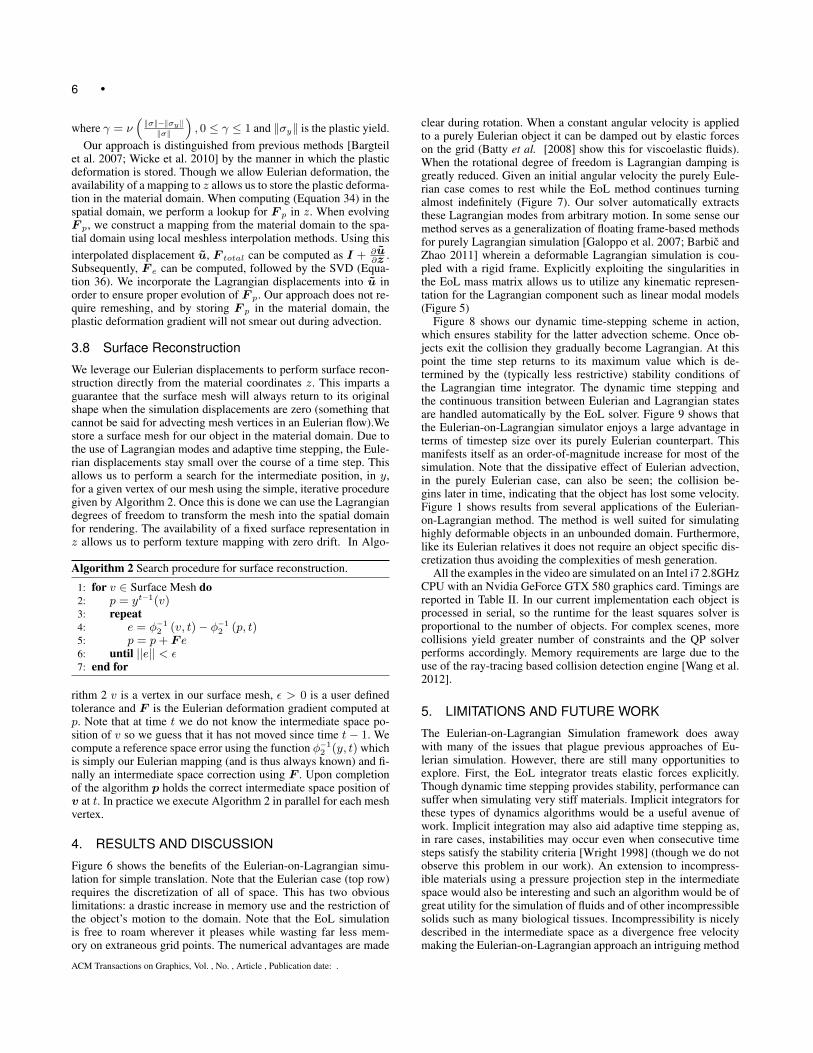
Figure 6 shows the benefits of the Eulerian-on-Lagrangian simu-lation for simple translation. Note that the Eulerian case (top row)requires the discretization of all of space. This has two obviouslimitations: a drastic increase in memory use and the restriction ofthe object’s motion to the domain. Note that the EoL simulationis free to roam wherever it pleases while wasting far less mem-ory on extraneous grid points. The numerical advantages are made

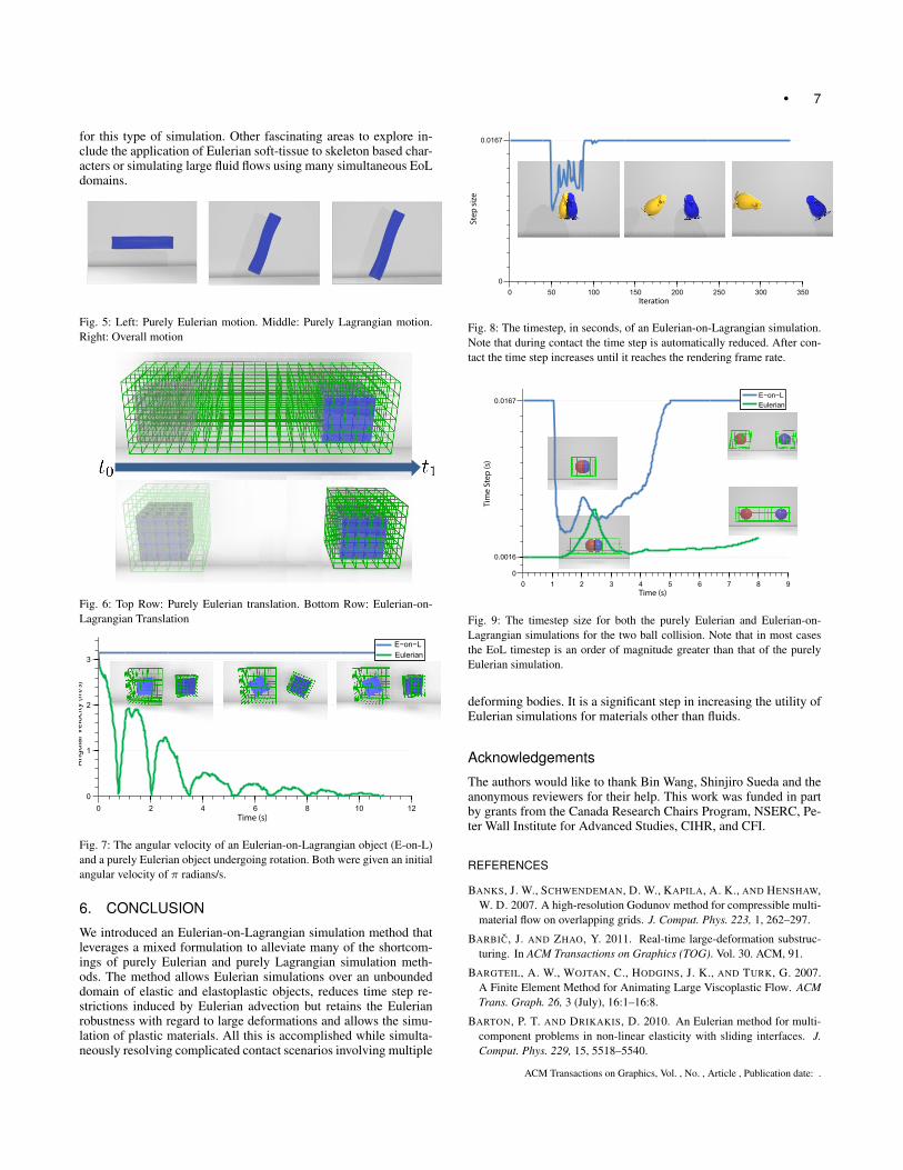
clear during rotation. When a constant angular velocity is appliedto a purely Eulerian object it can be damped out by elastic forceson the grid (Batty et al. [2008] show this for viscoelastic fluids).When the rotational degree of freedom is Lagrangian damping isgreatly reduced. Given an initial angular velocity the purely Eule-rian case comes to rest while the EoL method continues turningalmost indefinitely (Figure 7). Our solver automatically extractsthese Lagrangian modes from arbitrary motion. In some sense ourmethod serves as a generalization of floating frame-based methodsfor purely Lagrangian simulation [Galoppo et al. 2007; Barbic andZhao 2011] wherein a deformable Lagrangian simulation is cou-pled with a rigid frame. Explicitly exploiting the singularities inthe EoL mass matrix allows us to utilize any kinematic represen-tation for the Lagrangian component such as linear modal models(Figure 5)

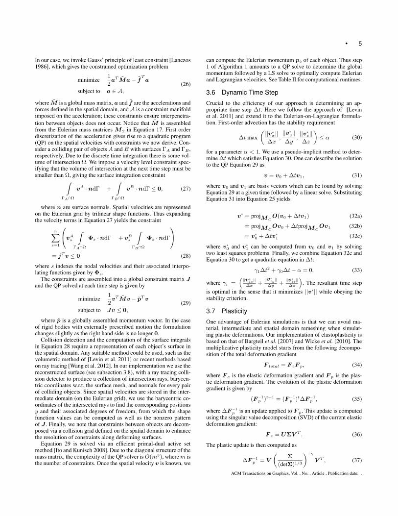
Figure 8 shows our dynamic time-stepping scheme in action,which ensures stability for the latter advection scheme. Once ob-jects exit the collision they gradually become Lagrangian. At thispoint the time step returns to its maximum value which is de-termined by the (typically less restrictive) stability conditions ofthe Lagrangian time integrator. The dynamic time stepping andthe continuous transition between Eulerian and Lagrangian statesare handled automatically by the EoL solver. Figure 9 shows thatthe Eulerian-on-Lagrangian simulator enjoys a large advantage interms of timestep size over its purely Eulerian counterpart. Thismanifests itself as an order-of-magnitude increase for most of thesimulation. Note that the dissipative effect of Eulerian advection,in the purely Eulerian case, can also be seen; the collision be-gins later in time, indicating that the object has lost some velocity.Figure 1 shows results from several applications of the Eulerian-on-Lagrangian method. The method is well suited for simulatinghighly deformable objects in an unbounded domain. Furthermore,like its Eulerian relatives it does not require an object specific dis-cretization thus avoiding the complexities of mesh generation.

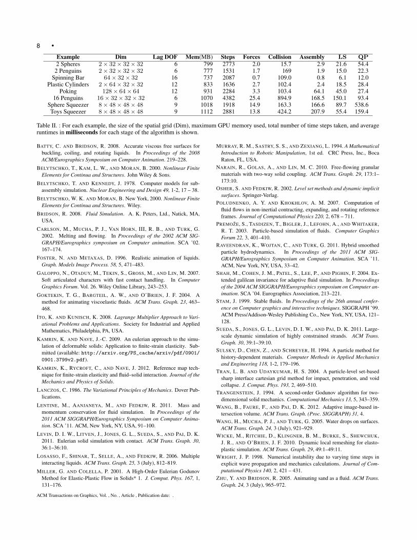
All the examples in the video are simulated on an Intel i7 2.8GHzCPU with an Nvidia GeForce GTX 580 graphics card. Timings arereported in Table II. In our current implementation each object isprocessed in serial, so the runtime for the least squares solver isproportional to the number of objects. For complex scenes, morecollisions yield greater number of constraints and the QP solverperforms accordingly. Memory requirements are large due to theuse of the ray-tracing based collision detection engine [Wang et al.2012].

5. LIMITATIONS AND FUTURE WORK

The Eulerian-on-Lagrangian Simulation framework does awaywith many of the issues that plague previous approaches of Eu-lerian simulation. However, there are still many opportunities toexplore. First, the EoL integrator treats elastic forces explicitly.Though dynamic time stepping provides stability, performance cansuffer when simulating very stiff materials. Implicit integrators forthese types of dynamics algorithms would be a useful avenue ofwork. Implicit integration may also aid adaptive time stepping as,in rare cases, instabilities may occur even when consecutive timesteps satisfy the stability criteria [Wright 1998] (though we do notobserve this problem in our work). An extension to incompress-ible materials using a pressure projection step in the intermediatespace would also be interesting and such an algorithm would be ofgreat utility for the simulation of fluids and of other incompressiblesolids such as many biological tissues. Incompressibility is nicelydescribed in the intermediate space as a divergence free velocitymaking the Eulerian-on-Lagrangian approach an intriguing method

ACM Transactions on Graphics, Vol. , No. , Article , Publication date: .

• 7

for this type of simulation. Other fascinating areas to explore in-clude the application of Eulerian soft-tissue to skeleton based char-acters or simulating large fluid flows using many simultaneous EoLdomains.

Fig. 5: Left: Purely Eulerian motion. Middle: Purely Lagrangian motion.Right: Overall motion

Fig. 6: Top Row: Purely Eulerian translation. Bottom Row: Eulerian-on-Lagrangian Translation

0 2 4 6 8 10 120

1

2

3

Time (s)

Ang

ular

Vel

ocity

(m/s

)

E−on−LEulerian

Fig. 7: The angular velocity of an Eulerian-on-Lagrangian object (E-on-L)and a purely Eulerian object undergoing rotation. Both were given an initialangular velocity of π radians/s.

6. CONCLUSION

We introduced an Eulerian-on-Lagrangian simulation method thatleverages a mixed formulation to alleviate many of the shortcom-ings of purely Eulerian and purely Lagrangian simulation meth-ods. The method allows Eulerian simulations over an unboundeddomain of elastic and elastoplastic objects, reduces time step re-strictions induced by Eulerian advection but retains the Eulerianrobustness with regard to large deformations and allows the simu-lation of plastic materials. All this is accomplished while simulta-neously resolving complicated contact scenarios involving multiple

0 50 100 150 200 250 300 3500

0.0167

Iteration

Step

siz

e

Fig. 8: The timestep, in seconds, of an Eulerian-on-Lagrangian simulation.Note that during contact the time step is automatically reduced. After con-tact the time step increases until it reaches the rendering frame rate.

0 1 2 3 4 5 6 7 8 90

0.0016

0.0167

Time (s)

Tim

e St

ep (s

)

E−on−LEulerian

Fig. 9: The timestep size for both the purely Eulerian and Eulerian-on-Lagrangian simulations for the two ball collision. Note that in most casesthe EoL timestep is an order of magnitude greater than that of the purelyEulerian simulation.

deforming bodies. It is a significant step in increasing the utility ofEulerian simulations for materials other than fluids.

Acknowledgements

The authors would like to thank Bin Wang, Shinjiro Sueda and theanonymous reviewers for their help. This work was funded in partby grants from the Canada Research Chairs Program, NSERC, Pe-ter Wall Institute for Advanced Studies, CIHR, and CFI.

REFERENCES

BANKS, J. W., SCHWENDEMAN, D. W., KAPILA, A. K., AND HENSHAW,W. D. 2007. A high-resolution Godunov method for compressible multi-material flow on overlapping grids. J. Comput. Phys. 223, 1, 262–297.

BARBIC, J. AND ZHAO, Y. 2011. Real-time large-deformation substruc-turing. In ACM Transactions on Graphics (TOG). Vol. 30. ACM, 91.

BARGTEIL, A. W., WOJTAN, C., HODGINS, J. K., AND TURK, G. 2007.A Finite Element Method for Animating Large Viscoplastic Flow. ACMTrans. Graph. 26, 3 (July), 16:1–16:8.

BARTON, P. T. AND DRIKAKIS, D. 2010. An Eulerian method for multi-component problems in non-linear elasticity with sliding interfaces. J.Comput. Phys. 229, 15, 5518–5540.

ACM Transactions on Graphics, Vol. , No. , Article , Publication date: .

8 •

Example Dim Lag DOF Mem(MB) Steps Forces Collision Assembly LS QP2 Spheres 2× 32× 32× 32 6 799 2773 2.0 15.7 2.9 21.6 54.4

2 Penguins 2× 32× 32× 32 6 777 1531 1.7 169 1.9 15.0 22.3Spinning Bar 64× 32× 32 16 737 2087 0.7 109.0 0.8 6.1 12.0

Plastic Cylinders 2× 64× 32× 32 12 833 1636 2.7 102.4 2.4 18.5 28.4Poking 128× 64× 64 12 931 2284 3.3 103.4 64.1 45.0 27.4

16 Penguins 16× 32× 32× 32 6 1070 4382 25.4 894.9 168.5 150.1 93.4Sphere Squeezer 8× 48× 48× 48 9 1018 1918 14.9 163.3 166.6 89.7 538.6Toys Squeezer 8× 48× 48× 48 9 1112 2881 13.8 424.2 207.9 55.4 159.4

Table II. : For each example, the size of the spatial grid (Dim), maximum GPU memory used, total number of time steps taken, and averageruntimes in milliseconds for each stage of the algorithm is shown.

BATTY, C. AND BRIDSON, R. 2008. Accurate viscous free surfaces forbuckling, coiling, and rotating liquids. In Proceedings of the 2008ACM/Eurographics Symposium on Computer Animation. 219–228.

BELYTSCHKO, T., KAM, L. W., AND MORAN, B. 2000. Nonlinear FiniteElements for Continua and Structures. John Wiley & Sons.

BELYTSCHKO, T. AND KENNEDY, J. 1978. Computer models for sub-assembly simulation. Nuclear Engineering and Design 49, 1-2, 17 – 38.

BELYTSCHKO, W. K. AND MORAN, B. New York, 2000. Nonlinear FiniteElements for Continua and Structures. Wiley.

BRIDSON, R. 2008. Fluid Simulation. A. K. Peters, Ltd., Natick, MA,USA.

CARLSON, M., MUCHA, P. J., VAN HORN, III, R. B., AND TURK, G.2002. Melting and flowing. In Proceedings of the 2002 ACM SIG-GRAPH/Eurographics symposium on Computer animation. SCA ’02.167–174.

FOSTER, N. AND METAXAS, D. 1996. Realistic animation of liquids.Graph. Models Image Process. 58, 5, 471–483.

GALOPPO, N., OTADUY, M., TEKIN, S., GROSS, M., AND LIN, M. 2007.Soft articulated characters with fast contact handling. In ComputerGraphics Forum. Vol. 26. Wiley Online Library, 243–253.

GOKTEKIN, T. G., BARGTEIL, A. W., AND O’BRIEN, J. F. 2004. Amethod for animating viscoelastic fluids. ACM Trans. Graph. 23, 463–468.

ITO, K. AND KUNISCH, K. 2008. Lagrange Multiplier Approach to Vari-ational Problems and Applications. Society for Industrial and AppliedMathematics, Philadelphia, PA, USA.

KAMRIN, K. AND NAVE, J.-C. 2009. An eulerian approach to the simu-lation of deformable solids: Application to finite-strain elasticity. Sub-mitted (available: http://arxiv.org/PS_cache/arxiv/pdf/0901/0901.3799v2.pdf).

KAMRIN, K., RYCROFT, C., AND NAVE, J. 2012. Reference map tech-nique for finite-strain elasticity and fluid–solid interaction. Journal of theMechanics and Physics of Solids.

LANCZOS, C. 1986. The Variational Principles of Mechanics. Dover Pub-lications.

LENTINE, M., AANJANEYA, M., AND FEDKIW, R. 2011. Mass andmomentum conservation for fluid simulation. In Proceedings of the2011 ACM SIGGRAPH/Eurographics Symposium on Computer Anima-tion. SCA ’11. ACM, New York, NY, USA, 91–100.

LEVIN, D. I. W., LITVEN, J., JONES, G. L., SUEDA, S., AND PAI, D. K.2011. Eulerian solid simulation with contact. ACM Trans. Graph. 30,36:1–36:10.

LOSASSO, F., SHINAR, T., SELLE, A., AND FEDKIW, R. 2006. Multipleinteracting liquids. ACM Trans. Graph. 25, 3 (July), 812–819.

MILLER, G. AND COLELLA, P. 2001. A High-Order Eulerian GodunovMethod for Elastic-Plastic Flow in Solids* 1. J. Comput. Phys. 167, 1,131–176.

MURRAY, R. M., SASTRY, S. S., AND ZEXIANG, L. 1994. A MathematicalIntroduction to Robotic Manipulation, 1st ed. CRC Press, Inc., BocaRaton, FL, USA.

NARAIN, R., GOLAS, A., AND LIN, M. C. 2010. Free-flowing granularmaterials with two-way solid coupling. ACM Trans. Graph. 29, 173:1–173:10.

OSHER, S. AND FEDKIW, R. 2002. Level set methods and dynamic implicitsurfaces. Springer-Verlag.

POLUDNENKO, A. Y. AND KHOKHLOV, A. M. 2007. Computation offluid flows in non-inertial contracting, expanding, and rotating referenceframes. Journal of Computational Physics 220, 2, 678 – 711.

PREMOZE, S., TASDIZEN, T., BIGLER, J., LEFOHN, A., AND WHITAKER,R. T. 2003. Particle-based simulation of fluids. Computer GraphicsForum 22, 3, 401–410.

RAVEENDRAN, K., WOJTAN, C., AND TURK, G. 2011. Hybrid smoothedparticle hydrodynamics. In Proceedings of the 2011 ACM SIG-GRAPH/Eurographics Symposium on Computer Animation. SCA ’11.ACM, New York, NY, USA, 33–42.

SHAH, M., COHEN, J. M., PATEL, S., LEE, P., AND PIGHIN, F. 2004. Ex-tended galilean invariance for adaptive fluid simulation. In Proceedingsof the 2004 ACM SIGGRAPH/Eurographics symposium on Computer an-imation. SCA ’04. Eurographics Association, 213–221.

STAM, J. 1999. Stable fluids. In Proceedings of the 26th annual confer-ence on Computer graphics and interactive techniques. SIGGRAPH ’99.ACM Press/Addison-Wesley Publishing Co., New York, NY, USA, 121–128.

SUEDA, S., JONES, G. L., LEVIN, D. I. W., AND PAI, D. K. 2011. Large-scale dynamic simulation of highly constrained strands. ACM Trans.Graph. 30, 39:1–39:10.

SULSKY, D., CHEN, Z., AND SCHREYER, H. 1994. A particle method forhistory-dependent materials. Computer Methods in Applied Mechanicsand Engineering 118, 1-2, 179–196.

TRAN, L. B. AND UDAYKUMAR, H. S. 2004. A particle-level set-basedsharp interface cartesian grid method for impact, penetration, and voidcollapse. J. Comput. Phys. 193, 2, 469–510.

TRANGENSTEIN, J. 1994. A second-order Godunov algorithm for two-dimensional solid mechanics. Computational Mechanics 13, 5, 343–359.

WANG, B., FAURE, F., AND PAI, D. K. 2012. Adaptive image-based in-tersection volume. ACM Trans. Graph. (Proc. SIGGRAPH) 31, 4.

WANG, H., MUCHA, P. J., AND TURK, G. 2005. Water drops on surfaces.ACM Trans. Graph. 24, 3 (July), 921–929.

WICKE, M., RITCHIE, D., KLINGNER, B. M., BURKE, S., SHEWCHUK,J. R., AND O’BRIEN, J. F. 2010. Dynamic local remeshing for elasto-plastic simulation. ACM Trans. Graph. 29, 49:1–49:11.

WRIGHT, J. P. 1998. Numerical instability due to varying time steps inexplicit wave propagation and mechanics calculations. Journal of Com-putational Physics 140, 2, 421 – 431.

ZHU, Y. AND BRIDSON, R. 2005. Animating sand as a fluid. ACM Trans.Graph. 24, 3 (July), 965–972.

ACM Transactions on Graphics, Vol. , No. , Article , Publication date: .