Embed Size (px)
Citation preview
*
ETSI ETR 284
TECHNICAL May 1996
REPORT
Source: ETSI TC-SMG Reference: DTR/SMG-020522P
ICS: 33.060.50
Key words: Digital cellular telecommunications system, Global System for Mobile communications (GSM)
Digital cellular telecommunications system (Phase 2);Radio link management in hierarchical networks
(GSM 05.22)
ETSIEuropean Telecommunications Standards Institute
ETSI Secretariat
Postal address: F-06921 Sophia Antipolis CEDEX - FRANCEOffice address: 650 Route des Lucioles - Sophia Antipolis - Valbonne - FRANCEX.400: c=fr, a=atlas, p=etsi, s=secretariat - Internet: [email protected]
Tel.: +33 92 94 42 00 - Fax: +33 93 65 47 16
Copyright Notification: No part may be reproduced except as authorized by written permission. The copyright and theforegoing restriction extend to reproduction in all media.
© European Telecommunications Standards Institute 1996 All rights reserved.
Page 2ETR 284: May 1996 (GSM 05.22 version 4.0.0)
Whilst every care has been taken in the preparation and publication of this document, errors in content,typographical or otherwise, may occur. If you have comments concerning its accuracy, please write to"ETSI Editing and Committee Support Dept." at the address shown on the title page.
Page 3ETR 284: May 1996 (GSM 05.22 version 4.0.0)
Contents
Foreword .......................................................................................................................................................7
1 Scope ..................................................................................................................................................9
2 References..........................................................................................................................................9
3 Abbreviations.......................................................................................................................................9
4 General................................................................................................................................................9
5 Hierarchical networks........................................................................................................................105.1 General ..............................................................................................................................105.2 Cell types ...........................................................................................................................10
5.2.1 Large cells .....................................................................................................105.2.2 Small cells .....................................................................................................105.2.3 Microcells ......................................................................................................10
6 Idle mode procedures .......................................................................................................................11
7 Examples of handover and RF power control algorithms. ................................................................117.1 General ..............................................................................................................................11
Annex A: Example 1 (Siemens AG) .......................................................................................................12
A.1 Introduction........................................................................................................................................12
A.2 Functional requirements....................................................................................................................12
A.3. BSS pre-processing and threshold comparisons ..............................................................................13A.3.1 Measurement averaging process ......................................................................................13A.3.2 Handover threshold comparison process ..........................................................................13
A.4 BSS decision algorithm .....................................................................................................................14
A.5 Additional O&M parameters stored for handover purposes in hierarchical networks .......................14
A.6. Bibliography.......................................................................................................................................15
Annex B: Example 2 (DeTeMobil) ..........................................................................................................16
B.1 Introduction........................................................................................................................................16
B.2 Definitions..........................................................................................................................................16B.2.1 Categories of cells .............................................................................................................16B.2.2 Classification of MS in connected mode............................................................................17
B.2.2.1 Classification in the lower layer .....................................................................17B.2.2.2 Classification in the middle layer or the upper layer ......................................17B.2.2.3 Loss of the "slow MS" or "quasi-stationary MS" status..................................18
B.3 Power Control Algorithm ...................................................................................................................18B.3.1 MS connected over a cell of the lower layer ......................................................................18B.3.2 MS connected over a cell of the middle layer or the upper layer .......................................18
B.4 Handover algorithm in a hierarchical cell structure ...........................................................................18B.4.1 MS connected over a cell of the lower layer ......................................................................18B.4.2 MS connected over a cell of the middle layer or the upper layer .......................................19
Page 4ETR 284: May 1996 (GSM 05.22 version 4.0.0)
B.4.3 Handover at borders of different cell structures ................................................................ 19
B.5 O&M-Parameter ............................................................................................................................... 19
B.6 State diagrams.................................................................................................................................. 20
Annex C: Example 3 (Alcatel) ................................................................................................................ 22
C.1 General description........................................................................................................................... 22C.1.1 Speed discrimination......................................................................................................... 22
C.2 Handover causes.............................................................................................................................. 23C.2.1 Emergency causes............................................................................................................ 23C.2.2 Better cell causes.............................................................................................................. 23
C.3 Dwell time in lower layer cells : ......................................................................................................... 23C.3.1 Serving cell = lower layer cell ............................................................................................ 23C.3.2 Serving cell = upper layer cell ........................................................................................... 23C.3.3 Mechanism of increasing / decreasing tdwell.................................................................... 23
C.4 Speed discrimination process :......................................................................................................... 24C.4.1 Serving cell = upperlayer cell ............................................................................................ 24C.4.2 Serving cell = lower layer cell ............................................................................................ 24
C.5 Representation of handovers............................................................................................................ 25C.5.1 Ideal behaviour : target cells are available ........................................................................ 25C.5.2 Real behaviour : target cells may not be available............................................................ 25
C.6 Emergency handover........................................................................................................................ 26C.6.1 Target cell = upper layer cell ............................................................................................. 26
C.7 Upper layer to lower layer cells handover......................................................................................... 26C.7.1 General principles ............................................................................................................. 26C.7.2 Homogeneity of speed discrimination in lower layer and upper layer cells ....................... 26
C.8 Minicells ............................................................................................................................................ 26C.8.1 Handover diagrams........................................................................................................... 27
C.9 O&M parameters .............................................................................................................................. 28
Annex D: Example 4 (France Telecom/CNET)...................................................................................... 29
D.1 Introduction ....................................................................................................................................... 29
D.2 Descriptions of the algorithm ............................................................................................................ 30
D.3 Handover causes.............................................................................................................................. 30D.3.1 emergency handover causes ............................................................................................ 30D.3.2 mobile speeds estimation causes ..................................................................................... 31
D.4 Mobile speeds estimations ............................................................................................................... 31D.4.1 Estimation of the field strength variations ......................................................................... 31
D.5 BSS decision algorithm :................................................................................................................... 32
D.6 O&M parameters .............................................................................................................................. 32
D.7 Examples.......................................................................................................................................... 33
D.8 State diagrams.................................................................................................................................. 35D.8.1 Case of a three layers hierarchical network ...................................................................... 35D.8.2 Case of a two layers hierarchical network......................................................................... 36
Page 5ETR 284: May 1996 (GSM 05.22 version 4.0.0)
Annex E: Simulation Model for Handover Performance Evaluation in Hierarchical Cell Structures.......38
E.1 Introduction........................................................................................................................................38
E.2 Mobile Environment...........................................................................................................................38
E.3 Radio Network Model ........................................................................................................................38E.3.1 Scenario 1: Hot Spot..........................................................................................................38E.3.2 Scenario 2: Line of Cells ....................................................................................................38E.3.3 Scenario 3: Manhattan Coverage ......................................................................................39
E.4 Propagation Model ............................................................................................................................39E.4.1 Upper Layer Path Loss ......................................................................................................39
E.4.1.1 Macrocells .....................................................................................................39E.4.1.2 Small cells ....................................................................................................40
E.4.2 Lower Layer Path Loss ......................................................................................................41E4.2.1 Line-of-sight Case .........................................................................................41E4.2.2 Non Line-of-sight Case..................................................................................42E.4.2.3 Shape of the level with the proposed path loss model ..................................42
E.4.3 Fading ................................................................................................................................43
E.5 Motion Model.....................................................................................................................................43
E.6 Handover Algorithms.........................................................................................................................43
E.7 Measurement Reporting....................................................................................................................44
E.8 Performance Criteria .........................................................................................................................44
E.9 Open Issues ......................................................................................................................................44
History..........................................................................................................................................................45
Page 6ETR 284: May 1996 (GSM 05.22 version 4.0.0)
Blank page
Page 7ETR 284: May 1996 (GSM 05.22 version 4.0.0)
Foreword
This ETSI Technical Report (ETR) has been produced by the Special Mobile Group (SMG) TechnicalCommittee of the European Telecommunications Standards Institute (ETSI).
This ETSI Technical Report (ETR) gives examples for the Radio sub-system link control to beimplemented in the Base Station System (BSS) and Mobile Switching Centre (MSC) of the GSM and DCS1800 systems in case hierarchical cell structures are employed.
This Draft ETR corresponds to GSM technical specification 05.22 version 4.0.0.
ETRs are informative documents resulting from ETSI studies which are not appropriate for EuropeanTelecommunication Standard (ETS) or Interim European Telecommunication Standard (I-ETS) status. AnETR may be used to publish material which is either of an informative nature, relating to the use or theapplication of ETSs or I-ETSs.

Page 8ETR 284: May 1996 (GSM 05.22 version 4.0.0)
Blank page
Page 9ETR 284: May 1996 (GSM 05.22 version 4.0.0)
1 Scope
This ETSI Technical Report (ETR) gives examples for the Radio sub-system link control to beimplemented in the Base Station System (BSS) and Mobile Switching Centre (MSC) of the GSM and DCS1800 systems in case hierarchical cell structures are employed.
Unless otherwise specified, references to GSM also include DCS 1800, and multiband systems ifoperated by a single operator.
2 References
This ETR incorporates by dated and undated reference, provisions from other publications. Thesereferences are cited at the appropriate places in the text and the publications are listed hereafter. Fordated references, subsequent amendments to or revisions of any of these publications apply to this ETRonly when incorporated in it by amendment or revision. For undated references, the latest edition of thepublication referred to applies.
[1] GSM 03.22 (ETS 300 535): "Digital cellular telecommunication system(Phase 2); Functions related to Mobile Station (MS) in idle mode".
[2] GSM 03.30: "Digital cellular telecommunication system (Phase 2); Radionetwork planning aspects".
[3] GSM 05.08 (ETS 300 578): "Digital cellular telecommunication system(Phase 2); Radio subsystem link control".
[4] GSM 01.04 (ETR 100): "Digital cellular telecommunication system (Phase 2);Abbreviations and acronyms".
3 Abbreviations
Abbreviations used in this ETR are listed in GSM 01.04 [4].
4 General
ETS 300 578 (GSM 05.08 [3]) specifies the radio sub system link control implemented in the MobileStation (MS), Base Station System (BSS) and Mobile Switching Centre (MSC) of the GSM and DCS 1800systems of the European digital cellular telecommunications system (Phase 2).
This ETR gives several examples of how the basic handover and RF power control algorithm as containedin (informative) Annex A to ETS 300 578 [3] can be enhanced to cope with the requirements on the radiosubsystem link control in hierarchical networks.
A hierarchical network is a network consisting of multiple layers of cells, allowing for an increased trafficcapacity and performance compared to a single layer network.
The radio sub-system link control aspects that are addressed are as follows:
- Handover;- RF Power control.
Page 10ETR 284: May 1996 (GSM 05.22 version 4.0.0)
5 Hierarchical networks
5.1 General
In a hierarchical, or microcellular network, traffic is supported on multiple layers of cells. Typically, anetwork operator could implement a layer consisting of microcells as a second layer in his existingnetwork consisting of large or small cells. The addition of this second layer would improve the capacityand coverage of his network.
In this ETR the following naming convention is used for the different layers. For a network consisting ofthree layers the layer using the biggest cells is the "upper layer ", followed by the "middle layer ", and thenthe "lower layer " which has the smallest cells. For a network consisting of two layers, only "upper layer "and "lower layer " are used.
The intention in a hierarchical network is to use the radio link control procedures to handle the majority ofthe traffic in the lower layer, i.e. the smallest cells, as this will limit interference and therefore improve thefrequency reuse.
However, a part of the traffic cannot always efficiently be handled in the lower layer. Examples are caseswhere the MS is moving fast (relative to the cell range), or where the coverage is insufficient, or where acell to make a handover to on the same level may not be available fast enough (going around corners,entering/leaving buildings).
5.2 Cell types
GSM 03.30 [2] distinguishes between three kinds of cells: large cells, small cells and micro cells. Themain difference between these kinds lies in the cell range, the antenna installation site, and thepropagation model applying:
5.2.1 Large cells
In large cells the base station antenna is installed above the maximum height of the surrounding roof tops;the path loss is determined mainly by diffraction and scattering at roof tops in the vicinity of the mobile i.e.the main rays propagate above the roof tops; the cell radius is minimally 1 km and normally exceeds 3 km.Hata's model and its extension up to 2000 MHz (COST231-Hata model) can be used to calculate the pathloss in such cells (GSM 03.30 [2] Annex B).
5.2.2 Small cells
For small cell coverage the antenna is sited above the median but below the maximum height of thesurrounding roof tops and so therefore the path loss is determined by the same mechanisms as stated inclause 5.1.1. However large and small cells differ in terms of maximum range and for small cells themaximum range is typically less than 1-3 km. In the case of small cells with a radius of less than 1 km theHata model cannot be used.
The COST 231-Walfish-Ikegami model (see GSM 03.30 [2] Annex B) gives the best approximation to thepath loss experienced when small cells with a radius of less than 5 km are implemented in urbanenvironments. It can therefore be used to estimate the BTS ERP required in order to provide a particularcell radius (typically in the range 200 m - 3 km).
5.2.3 Microcells
COST 231 defines a microcell as being a cell in which the base station antenna is mounted generallybelow roof top level. Wave propagation is determined by diffraction and scattering around buildings i.e. themain rays propagate in street canyons. COST 231 proposes an experimental model for microcellpropagation when a free line of sight exists in a street canyon (see GSM 03.30 [2]).
The propagation loss in microcells increases sharply as the receiver moves out of line of sight, forexample, around a street corner. This can be taken into account by adding 20 dB to the propagation lossper corner, up to two or three corners (the propagation being more of a guided type in this case). Beyond,the complete COST231-Walfish-Ikegami model as presented in annex B of GSM 03.30 [2] should beused.
Page 11ETR 284: May 1996 (GSM 05.22 version 4.0.0)
Microcells have a radius in the region of 200 to 300 metres and therefore exhibit different usage patternsfrom large and small cells.
6 Idle mode procedures
GSM 03.22 [1] outlines how idle mode operation shall be implemented. Further details are given inTechnical Specifications GSM 04.08 and GSM 05.08 [3].
A useful feature for hierarchical networks is that cell prioritisation, for Phase 2 MS, can be achieved duringcell reselection by the use of the reselection parameters optionally broadcast on the BCCH. Cells arereselected on the basis of a parameter called C2 and the C2 value for each cell is given a positive ornegative offset (CELL_RESELECT_OFFSET) to encourage or discourage MSs to reselect that cell. A fullrange of positive and negative offsets is provided to allow the incorporation of this feature into alreadyoperational networks.
The parameters used to calculate C2 are as follows:
a) CELL_RESELECT_OFFSET;
b) PENALTY_TIME;
When the MS places the cell on the list of the strongest carriers as specified in GSM 05.08 [3], itstarts a timer which expires after the PENALTY_TIME. This timer will be reset when the cell istaken off the list. For the duration of this timer, C2 is given a negative offset. This will tend toprevent fast moving MSs from selecting the cell.
c) TEMPORARY_OFFSET;
This is the amount of the negative offset described in (ii) above. An infinite value can be applied, buta number of finite values are also possible.
The permitted values of these parameters and the way in which they are combined to calculate C2 aredefined in GSM 05.08 [3].
7 Examples of handover and RF power control algorithms.
7.1 General
In the following annexes four examples of handover and power control algorithms are presented. All ofthese are considered sufficient to allow successful implementation in hierarchical or microcellularnetworks. None of these solutions is mandatory.
The "Description of algorithm " of each annex, contains a text as provided by the authors of thealgorithm. Any discussion on the algorithms is contained in a separate clause, "Discussion ofalgorithm" .
Page 12ETR 284: May 1996 (GSM 05.22 version 4.0.0)
Annex A: Example 1 (Siemens AG)
Description of algorithm
Source: Siemens AG
Date: 23.08.95
Subject: Fast Moving Mobiles
A.1 Introduction
This annex specifies an enhanced handover algorithm that may be implemented in GSM or DCS 1800hierarchical networks. In accordance with Clause 5 of this annex a hierarchical network is understood as anetwork utilizing large cells for the upper layer for wide area coverage, and a lower layer structure of smallor micro cells for capacity reasons. For the sake of simplicity the algorithm is described for hierarchicalnetworks consisting of two layers. Nevertheless the algorithm can be extended to a hierarchy comprisingseveral layers.
The algorithm is based upon the basic handover process, as described in GSM 05.08 [3], Annex A. Onlydifferences and supplements to the standard algorithms are explicitly described.
The aim of this annex is to show, how in hierarchical networks useless handovers can be avoided byallocating the mobiles, according to their speed, to the appropriate cell type. This goal is achieved bysteering the fast mobile stations to the upper layer structure (e.g. large cells), while ensuring that slowmobile subscribers are served by the lower layer structure (e.g. small or micro cells). A mobile station isconsidered as fast, if its sojourn time in a cell is short compared to a mean call holding time.
An important aspect of this advanced algorithm is, that there is no implication on the MS type. Theprocedures described in this annex, work in the same manner for Phase 2 as well as Phase 1 MS types.
A more comprehensive description of the advanced algorithm along with some investigation results basedon handover emulations in typical mixed cell scenarios is given in "Mobile Speed Sensitive Handover in aMixed Cell Environment" (see Bibliography).
A.2 Functional requirements
The present algorithm is based on the following additional assumptions:
- The upper layer structure (e.g. large cells) provides a contiguous wide area coverage for all MSpower classes to be supported by the network.
- The lower layer structure (e.g. small or micro cells) is fully embedded in the coverage area of upperlayer structure (e.g. large cells).
- The algorithm is based on both a power budget and absolute level criterion. Therefore both criteriashall be enabled simultaneously, giving a higher priority to the absolute level criterion.
Page 13ETR 284: May 1996 (GSM 05.22 version 4.0.0)
A.3. BSS pre-processing and threshold comparisons
A.3.1 Measurement averaging process
In a mixed cell environment one should take into account the different propagation conditions in large andsmall or micro cells, and the requirement for speeding up the handover decision, when a handover out of asmall cell is pending (especially, with the street corner effect in micro cells), an excessive delay of thehandover detection can cause a loss of the connection. Regarding this, the following items are recommended:
a) Apply different values for the averaging parameters in large and small or micro cells, respectively.
b) Define separate averaging parameters applicable to RXLEV and RXLEV_NCELL(n), respectively.
c) The BSS shall evaluate the Power Budget PBGT(n) using the averaging process defined forRXLEV_NCELL(n).
A.3.2 Handover threshold comparison process
The Handover threshold comparison process is similar to the process described in GSM 05.08 [3], AnnexA, except for section e) in A.3.2.2, which is modified as follows:
e) Comparison of PBGT(n) with the variable hysteresis margin HO_MARGIN_TIME(n). If the processis employed, the action to be taken is as follows:
If PBGT(n) > HO_MARGIN_TIME(n) a handover, cause PBGT(n), might be required.
In a hierarchical network this comparison enables handover into the lower layer structure (e.g. small ormicro cells) to be performed for slow mobile stations, while fast-moving ones remain served by the upperlayer structure (e.g. large cells).
The variable hysteresis margin is defined by:
HO_MARGIN_TIME(n) = HO_MARGIN(n) + HO_STATIC_OFFSET(n) - HO_DYNAMIC_OFFSET(n) * H(T(n) -DELAY_TIME(n)).
In addition to the HO_MARGIN(n) as defined in table A.1 of GSM 05.08 [3] except that the range hasbeen extended to (-24, 24 dB), the variable hysteresis margin comprises:
- a static offset, HO_STATIC_OFFSET(n);
- a dynamic offset, HO_DYNAMIC_OFFSET(n); and
- a delay time interval, DELAY_TIME(n).
The parameters are related to cells of the lower layer structure only.
T(n) is the time that has elapsed since the point at which the mobile station has entered the coverage areaof cell n in the lower layer structure.
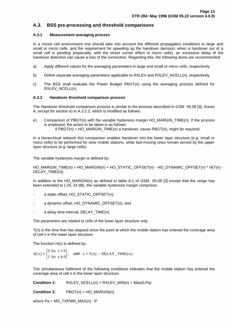
The function H(x) is defined by:
H x for x
for x( ) =
<≥
RST
UVW
0
1
0
0, with x T(n) - DELAY_ TIME(n)= .
The simultaneous fulfilment of the following conditions indicates that the mobile station has entered thecoverage area of cell n in the lower layer structure:
Condition 1: RXLEV_NCELL(n) > RXLEV_MIN(n) + Max(0,Pa)
Condition 2: PBGT(n) > HO_MARGIN(n),
where Pa = MS_TXPWR_MAX(n) - P.
Page 14ETR 284: May 1996 (GSM 05.22 version 4.0.0)
If both conditions are true, a timer T(n) shall be started. If any of these conditions gets false, before thetimer expiry, the timer shall be stopped and reset.
NOTE 1: HO_MARGIN_TIME(n) = HO_MARGIN(n) + HO_STATIC_OFFSET(n) for those cellsof the lower layer structure, whose timer has not yet been started or is still running. Ahigh value of HO_STATIC_OFFSET effectively prevents a handover into therespective cell of the lower layer structure during the run time of the timer for that cell.
NOTE 2: HO_MARGIN_TIME(n) =HO_MARGIN(n) + HO_STATIC_OFFSET(n)
- HO_DYNAMIC_OFFSET(n)
for those cells of the lower layer structure, whose timer has expired. This is the marginfixing the cell borders and replacing the usual HO_MARGIN(n) within the standardhandover of GSM 05.08 [3], Annex A.
On timer expiry the reduced HO_MARGIN_TIME(n) allows for a power budgethandover into a cell of the lower layer structure for a slow moving mobile which isexpected to be still in the coverage area of that cell.
On the contrary, a fast moving mobile is expected to have left the coverage area of anembedded cell of the lower layer structure while the timer for that cell is still runningand therefore Condition 1 or 2 (or both) will be violated, thus preventing a handoverrequest for a fast moving mobile into that cell of the lower layer structure.Consequently, fast moving mobiles are kept on the upper layer structure.
NOTE 3: A fast moving mobile connected to a cell of the lower layer structure (e.g. a phase 1mobile being not able to run the reselection algorithm in idle mode or a mobile havingchanged its speed) is steered to the upper layer structure by requesting for it a rescuehandover based on the absolute level criterion.
NOTE 4: HO_MARGIN(n) defines the location of timer start. Choosing small or even negativevalues results in an early timer start and thereby avoiding cell border displacement andinterference problems. Setting HO_MARGIN(n) to large negative values effectivelycancels Condition 2, and consequently the timer start is triggered only by Condition 1such that the cell borders on the lower layer structure are independent of the cell sitepositions with respect to the cell sites in the upper layer structure.
A.4 BSS decision algorithm
The BSS decision algorithm described in GSM 05.08 [3], Annex A, may be employed after replacingHO_MARGIN(n) by the corresponding HO_MARGIN_TIME(n) in equation (2) of Annex A. In combinationwith suitable parameter settings this results in the mobile speed sensitive handover functionalityreferenced above.
A.5 Additional O&M parameters stored for handover purposes in hierarchicalnetworks
HO_STATIC_OFFSET(n) A parameter used to apply a positive offset to HO_MARGIN(n) in order toprevent a handover request into cell n of the lower layer structure.
Range: 0 - 127 dB)
Step Size: 1 dB.
Admin. for: HO_STATIC_OFFSET(n) for each neighbour cell of the lower layer structure (n = 1 - 32)
Page 15ETR 284: May 1996 (GSM 05.22 version 4.0.0)
HO_DYNAMIC_OFFSET(n) A parameter used to partially or fully compensate the HO_STATIC_OFFSET(n) for cell n of the lower layer structure. This parameter gets active after the time interval DELAY_TIME(n).
Range: 0 - 127 dB)
Step Size: 1 dB.
Admin. for: HO_DYNAMIC_OFFSET(n) for each neighbour cell of the lower layer structure (n = 1 - 32)
DELAY_TIME(n) Time interval used to delay the handover decision into cell n of the lower layer structure to enable differentiation between fast and slow mobile stationsin the handover decision process.
Range: 0 - 255 Tsacch
Step Size: 1 Tsacch
Admin. for: DELAY_TIME(n) for each neighbour cell of the lower layer structure (n = 1 - 32)
NOTE: These parameters apply only for cells of the lower layer structure.
A.6. Bibliography
1) K. Ivanov, G. Spring, "Mobile Speed Sensitive Handover in a Mixed CellEnvironment", in Proc. IEEE 45th Veh. Technol. Conf., VTC 1995, pp. 892-896.
Page 16ETR 284: May 1996 (GSM 05.22 version 4.0.0)
Annex B: Example 2 (DeTeMobil)
Description of algorithm
Source: DeTeMobilDate: 21.08.1995Subject: High speed MS
B.1 Introduction
In order to provide significantly more traffic capacity in GSM networks, the average cell size has tobecome smaller. The reduction in cell size, however, should neither limit the mobility of the MS nor the MSspeed. On the one hand problems will occur if the MS are so fast, that the time they stay in a small cell istoo short for the radio link control procedures to be carried out efficiently and effectively and on the otherhand if it is necessary to handover a MS to predetermined target cells very quickly if the received RFsignal level of a radio connection is changing rapidly in a radio environment of small cells.
To give good performance to all MS, the network has to be built up using cells of different sizes at oneplace, i.e. a hierarchical cell structure. The network provides a multi-coverage. Dependent on the MSspeed, the MS shall be handled by a cell with a suitable size.
The procedures to achieve this for an MS in idle mode are described in GSM 03.22 [1].
The radio link control procedures in the concept of a hierarchical cell structure are independent of theconnections to MSC and BSC.
In the following the procedures to handle MS in connected mode for a hierarchical cell structure are given.
B.2 Definitions
B.2.1 Categories of cells
A hierarchical cell structure is built up from different layers of cells. The structure shall allow at least threelayers: the lower layer, the middle layer and the upper layer(see note). If only two layers are planned, thelower layer and middle layer are used. It is emphasised that the relation to other cells determines theassignment to a layer in the hierarchical cell structure. The absolute size of a cell is not a criterion.
NOTE: An example for the use of middle and upper layer is as follows:
- Middle layer: Layer with sufficient capacity to handle the traffic for fast movingMS.
- Upper layer: ‘Umbrella Cells’ of the middle layer, here only handover traffic shallbe supported, when cells of the middle layer are not available.
The layer to which a cell in a hierarchical cell structure is assigned is set by the O&M-parameterCELL_LEVEL.
Cells that do not belong into a hierarchical structure (single layer) have the CELL_LEVEL 'standard layer'that is the default level if details concerning the CELL_LEVEL are missing.
The parameter CELL_LEVEL has a range from 0 to 15(see note) and is allocated for each radio cell. Thecoding is given in clause B.5. In each radio cell the own level, and the levels for all neighbour cells, as inthe BA(SACCH), are known.
NOTE: Possible reasons to introduce new layers may be: pico cells, specific servicessupported only in one layer, multiband systems etc.
Page 17ETR 284: May 1996 (GSM 05.22 version 4.0.0)
B.2.2 Classification of MS in connected mode
For radio link control purposes in a hierarchical cell structure, an MS in connected mode is classified by aset of at least [eight] status-fields. The set is called MS_STATUS. With one of these fields: MS_SPEED,MS are distinguished between "fast MS", "slow MS" and "quasi-stationary MS". All other fields of the setare for future use (see note)
NOTE: Possible details given in the fields that are for future use are: multiple band, GPRS,EFR etc..
MS_STATUS is used in decisions of the power control process.
At the establishment of an RR-connection MS_SPEED is set to the default value "fast MS", except forPhase 2 MS if establishment is in cells of the lower layer in which the path loss criterion C2 is activated.Then MS_SPEED is set to "slow MS".
The speed classification can be enabled/disabled by the flag EN_MS_SPEED.
If the flag EN_MS_SPEED is set to 0 (disabled) in a cell of the lower layer the classification is omitted, andthe status of the MS in this cell will not be changed. At the establishment of an RR-connection all MS areset to the MS_SPEED default value "fast MS". During handover the MS shall keep the status of theprevious cell.
In cells of the middle layer or the upper layer, all cells of the lower layer with the flag EN_MS_SPEEDdisabled, are excluded from the classification procedure as described in subclause B.2.2.2.
B.2.2.1 Classification in the lower layer
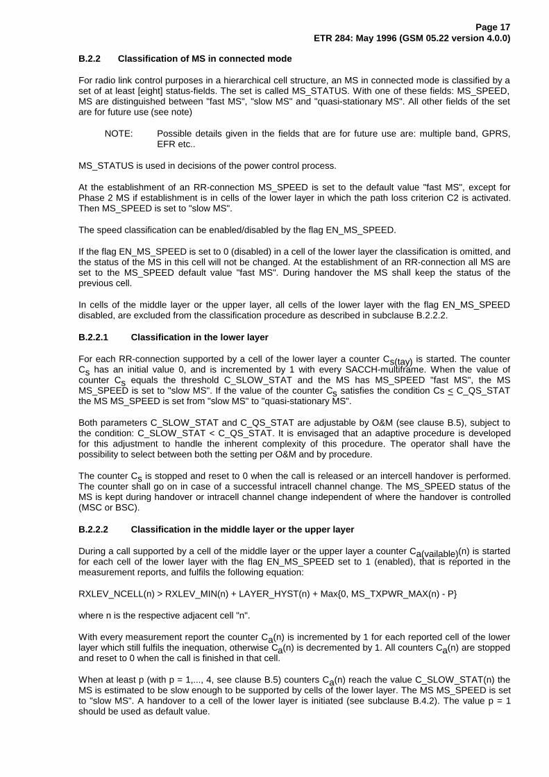
For each RR-connection supported by a cell of the lower layer a counter Cs(tay) is started. The counterCs has an initial value 0, and is incremented by 1 with every SACCH-multiframe. When the value ofcounter Cs equals the threshold C_SLOW_STAT and the MS has MS_SPEED "fast MS", the MSMS_SPEED is set to "slow MS". If the value of the counter Cs satisfies the condition Cs < C_QS_STATthe MS MS_SPEED is set from "slow MS" to "quasi-stationary MS".
Both parameters C_SLOW_STAT and C_QS_STAT are adjustable by O&M (see clause B.5), subject tothe condition: C_SLOW_STAT < C_QS_STAT. It is envisaged that an adaptive procedure is developedfor this adjustment to handle the inherent complexity of this procedure. The operator shall have thepossibility to select between both the setting per O&M and by procedure.
The counter Cs is stopped and reset to 0 when the call is released or an intercell handover is performed.The counter shall go on in case of a successful intracell channel change. The MS_SPEED status of theMS is kept during handover or intracell channel change independent of where the handover is controlled(MSC or BSC).
B.2.2.2 Classification in the middle layer or the upper layer
During a call supported by a cell of the middle layer or the upper layer a counter Ca(vailable)(n) is startedfor each cell of the lower layer with the flag EN_MS_SPEED set to 1 (enabled), that is reported in themeasurement reports, and fulfils the following equation:
RXLEV_NCELL(n) > RXLEV_MIN(n) + LAYER_HYST(n) + Max{0, MS_TXPWR_MAX(n) - P}
where n is the respective adjacent cell "n".
With every measurement report the counter Ca(n) is incremented by 1 for each reported cell of the lowerlayer which still fulfils the inequation, otherwise Ca(n) is decremented by 1. All counters Ca(n) are stoppedand reset to 0 when the call is finished in that cell.
When at least p (with p = 1,..., 4, see clause B.5) counters Ca(n) reach the value C_SLOW_STAT(n) theMS is estimated to be slow enough to be supported by cells of the lower layer. The MS MS_SPEED is setto "slow MS". A handover to a cell of the lower layer is initiated (see subclause B.4.2). The value p = 1should be used as default value.
Page 18ETR 284: May 1996 (GSM 05.22 version 4.0.0)
NOTE: p > 1 gives the possibility in special cases, where information on the velocity of MS isnot reliable, e.g. in the surroundings of traffic lights, to tighten the requirement for thehandover towards the lower layer of MS. p=1 is sufficient in most cases.
B.2.2.3 Loss of the "slow MS" or "quasi-stationary MS" status
During an RR-connection, when a handover from a cell of the lower layer to a cell of the middle layer orthe upper layer is performed, the MS MS_SPEED is set to "fast MS". This happens when a handover withcause RXLEV, RXQUAL or distance occurs before the counter Cs reaches the value C_SLOW_STAT.
Furthermore, in the case that no radio resource is available in one of the higher layers, and the handoveris performed to a cell of the lower layer, the MS MS_SPEED is set to "fast MS".
B.3 Power Control Algorithm
B.3.1 MS connected over a cell of the lower layer
In cells of the lower layer the power control algorithm shall be dependent on the MS MS_SPEED.
For a "fast MS" power control shall be [disabled]. The maximum allowed power level for that cell and forthe class of MS has to be used by MS and BSS.
For MS with MS_SPEED "slow MS" or "quasi-stationary MS" the power control process as described inAnnex A of 05.08 [3] is used, with the following proviso:
In case of a MS with MS_SPEED "quasi-stationary MS" the power control ranges and the averagingperiods are the same as used in the middle layer/upper layer or standard layer.
For MS with MS_SPEED "slow MS" the maximum allowed power in uplink and downlink may be reducedonly by [five] 2 dB steps. For slow MS an separate set of power control parameters, for example forPOW_INCR/RED_STEP_SIZE and P_CON_INTERVAL shall be used.
B.3.2 MS connected over a cell of the middle layer or the upper layer
For all MS connected via the middle- or upper layer the power control process as described in the 05.08[3] are used.
B.4 Handover algorithm in a hierarchical cell structure
B.4.1 MS connected over a cell of the lower layer
After the successful establishment of an RR-connection in a cell of the lower layer, the counter Cs isstarted for this connection. In addition to the classification of MS (see subclause B.2.2), the counter isused to measure the time an MS stays in the cell of the lower layer.
If a handover with cause RXLEV, RXQUAL or distance occurs before Cs has reached the thresholdC_SLOW_STAT, the handover is performed with preference to a cell of the middle layer. Only if no TCHis available in the middle layer, a cell of the upper layer is selected as handover-candidate. In case there isno cell or TCH available in the higher layers, the handover candidate shall be a cell from the lower layer.As long as the value of Cs is smaller than C_SLOW_STAT a handover cause PBGT is not possible.
When Cs is equal or greater than C_SLOW_STAT all handover types are possible to all cells of the lowerlayer regardless of the MS MS_SPEED ("slow MS" or "quasi-stationary MS"). If no cell of the lower layer isavailable for a forced handover, the handover candidate shall be a cell from the middle layer or in case ofunavailability from the upper layer. Only under this condition the MS retains MS_SPEED "slow MS" or"quasi-stationary MS" during a handover from lower layer to either middle layer or upper layer. In case of aPBGT-handover, the handover candidate list may only contain cells from the lower layer.
Page 19ETR 284: May 1996 (GSM 05.22 version 4.0.0)
B.4.2 MS connected over a cell of the middle layer or the upper layer
For RR-connections supported by cells of the middle layer or the upper layer a standard handoverprocedure as specified e.g. in Annex A of 05.08 [3] is used with the additions and restrictions as follows.
The counter Ca(n) that is started for each cell of the lower layer (see subclause B.2.2), is used to trigger ahandover from an actual serving cell of a higher level to a cell of the lower layer.
When at least p counters Ca(n) reach the value C_SLOW_STAT(n) the MS is estimated to be slowenough, so that it can be supported by cells of the lower layer.
As long as the above condition is not fulfilled, the handover from a cell of the middle layer/upper layer to acell of the lower layer is not allowed with the exception for the handover causes RXLEV, RXQUAL orDISTANCE that only the lower layer has free resources.
When Ca(n) reaches the value C_SLOW_STAT(n) for at least p cells of the lower layer, a handover isinitiated towards the lower layer. All available cells of the lower layer are possible handover candidates.The handover shall be performed to that cell of the lower layer which has the best PBGT.
If the p-th counter Ca(n) reaches the value C_SLOW_STAT(n) at the same time that a handover causePBGT is recognised, the PBGT-handover has to be performed.
B.4.3 Handover at borders of different cell structures
A border appears where an area with an hierarchical cell structure adjoins an area consisting of a singlelayer of cells.
For an MS that moves from the area with an hierarchical cell structure into the area with a single layer ofcells, these cells of the standard layer are treated like cells of the middle layer.
In case of an MS moving from the single standard layer towards the hierarchical cell structure, for thepurpose of radio link purposes there is no distinction between the cells of the hierarchical cell structure.This is because no information is available on the hierarchical structure in the standard layer.
B.5 O&M-Parameter
CELL_LEVEL Hierarchy level of serving cellRange: 0 - 15Step size: 1Coding: 0: standardlayer
1: lower layer2: middle layer3: upper layer4 - 15: for future use
Used in: BSCAdmin. for: CELL_LEVEL for each cell
CELL_LEVEL_NC(n) Hierarchy level of n-th neighbour celln: 1 - 32Range: 0 - 15Step size: 1Coding: 0: standardlayer
1: lower layer2: middle layer3: upper layer4 - 15: for future use
Used in: BSCAdmin. for: CELL_LEVEL_NC(n) for each adjacent cell n of a radio cell
EN_MS_SPEED ENable classification of MS regarding SPEEDCoding: 1: enable feature
0: disable featureUsed in: BSCAdmin. for: each cell
Page 20ETR 284: May 1996 (GSM 05.22 version 4.0.0)
C_SLOW_STAT Time an MS has to stay in a cell of the lower layer until MS_SPEED is set to"slow MS"Range: 0 - 255 TSACCHStep Size: 1 TSACCHUsed in: BSCAdmin. for: C_SLOW_STAT for each cell of the lower layerConditions: 1. C_SLOW_STAT < C_QS_STAT
2. C_SLOW_STAT = C_SLOW_STAT(n) related to one cell
C_SLOW_STAT(n) Time neighbour cell n of the lower layer has to be reported as suitable by an MSsupported by the middle layer or upper layer until MS_SPEED is set to "slowMS"Range: 0 - 255 TSACCHStep Size: 1 TSACCHUsed in: BSCAdmin. for: C_SLOW_STAT(n) for each adjacent lower layer cell n of a
middle layer or upper layer cell (n = 1 - 32)Conditions: 1. C_SLOW_STAT < C_QS_STAT
2. C_SLOW_STAT = C_SLOW_STAT(n) related to one cell
C_QS_STAT Time an MS has to stay in a cell of the lower layer until MS_SPEED is set to"Quasi-stationary MS"Range: 0 - 510 TSACCHStep Size: 2 TSACCHUsed in: BSCAdmin. for: each cellCondition: C_QS_STAT > C_SLOW_STAT
LAYER_HYST(n) Hysteresis for handover from the middle layer/upper layer to the lower layerRange: 0 - [31] dBStep Size: 1 dBUsed in: BSCAdmin. for: each neighbour cell
p number of cells that has to fulfil the inequation to estimate an MS as slowRange: 1 - 4Step Size: 1Used in: BSCAdmin. for: each cell of the middle layer or upper layer
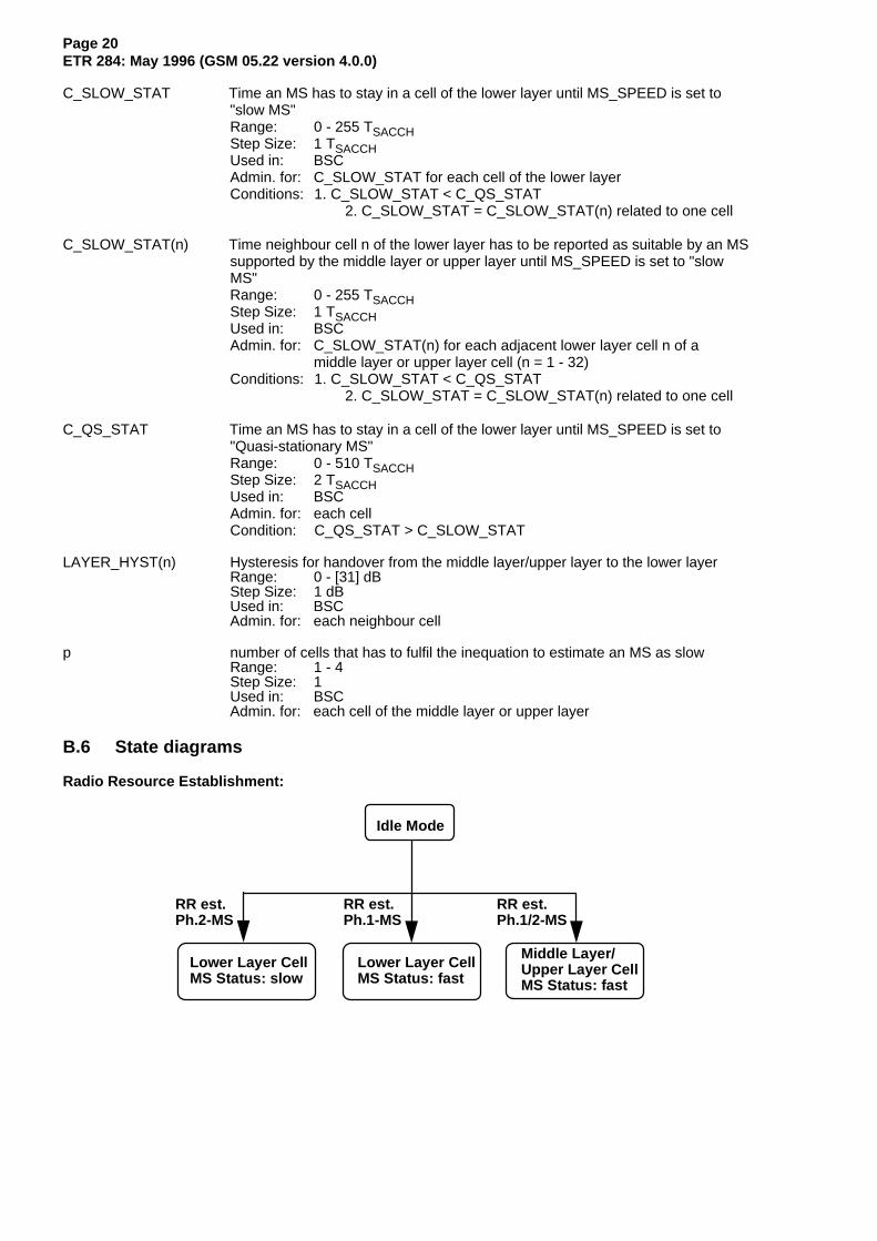
B.6 State diagrams
Radio Resource Establishment:
RR est.Ph.1/2-MS
RR est.Ph.1-MS
RR est.Ph.2-MS
Idle Mode
Middle Layer/Upper Layer CellMS Status: fast
Lower Layer CellMS Status: fast
Lower Layer CellMS Status: slow
Page 21ETR 284: May 1996 (GSM 05.22 version 4.0.0)
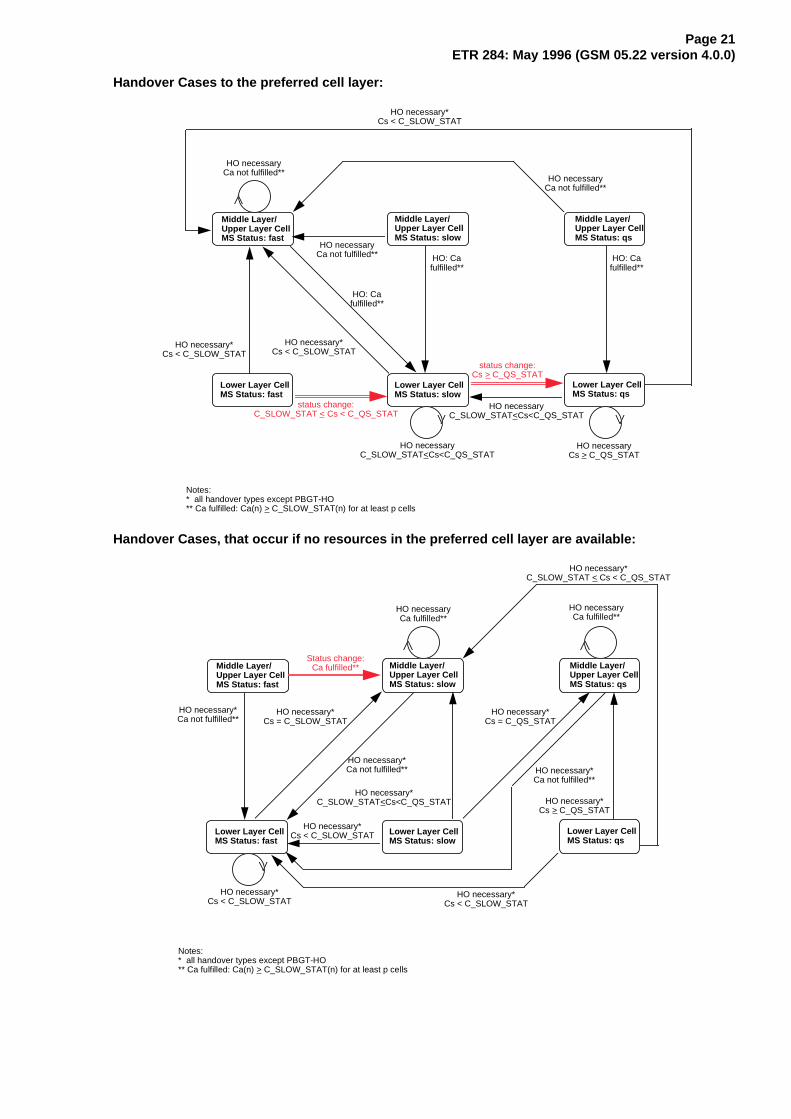
Handover Cases to the preferred cell layer:
HO necessary*Cs < C_SLOW_STAT
HO necessary*Cs < C_SLOW_STAT
HO necessaryC_SLOW_STAT<Cs<C_QS_STAT
status change:C_SLOW_STAT < Cs < C_QS_STAT
HO necessaryCa not fulfilled**
status change:Cs > C_QS_STAT
HO necessary*Cs < C_SLOW_STAT
HO: Cafulfilled**
Lower Layer CellMS Status: slow
Lower Layer CellMS Status: qs
Lower Layer CellMS Status: fast
Middle Layer/Upper Layer CellMS Status: slow
Middle Layer/Upper Layer CellMS Status: fast
Middle Layer/Upper Layer CellMS Status: qs
HO: Cafulfilled**
HO necessaryCa not fulfilled**
HO necessaryC_SLOW_STAT<Cs<C_QS_STAT
HO necessaryCs > C_QS_STAT
HO: Cafulfilled**
HO necessaryCa not fulfilled**
Notes:* all handover types except PBGT-HO** Ca fulfilled: Ca(n) > C_SLOW_STAT(n) for at least p cells
Handover Cases, that occur if no resources in the preferred cell layer are available:
HO necessary*Cs < C_SLOW_STAT
HO necessary*C_SLOW_STAT < Cs < C_QS_STAT
HO necessary*Cs < C_SLOW_STAT
HO necessary*Cs < C_SLOW_STAT
HO necessary*Ca not fulfilled**
Lower Layer CellMS Status: slow
Lower Layer CellMS Status: qs
Lower Layer CellMS Status: fast
Middle Layer/Upper Layer CellMS Status: slow
Middle Layer/Upper Layer CellMS Status: fast
Middle Layer/Upper Layer CellMS Status: qs
HO necessaryCa fulfilled**
HO necessaryCa fulfilled**
HO necessary*Ca not fulfilled**
HO necessary*C_SLOW_STAT<Cs<C_QS_STAT
HO necessary*Cs = C_QS_STAT
HO necessary*Cs = C_SLOW_STAT
HO necessary*Cs > C_QS_STAT
Status change:Ca fulfilled**
Notes:* all handover types except PBGT-HO** Ca fulfilled: Ca(n) > C_SLOW_STAT(n) for at least p cells
HO necessary*Ca not fulfilled**
Page 22ETR 284: May 1996 (GSM 05.22 version 4.0.0)
Annex C: Example 3 (Alcatel)
Description of algorithm
C.1 General description
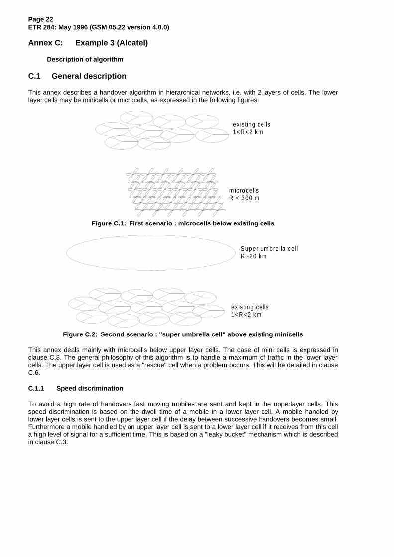
This annex describes a handover algorithm in hierarchical networks, i.e. with 2 layers of cells. The lowerlayer cells may be minicells or microcells, as expressed in the following figures.
ex is ting ce lls1<R <2 km
m icro ce llsR < 3 00 m
Figure C.1: First scenario : microcells below existing cells
S upe r u m bre lla ce llR ~20 km
ex is ting ce lls1<R <2 km
Figure C.2: Second scenario : "super umbrella cell" above existing minicells
This annex deals mainly with microcells below upper layer cells. The case of mini cells is expressed inclause C.8. The general philosophy of this algorithm is to handle a maximum of traffic in the lower layercells. The upper layer cell is used as a "rescue" cell when a problem occurs. This will be detailed in clauseC.6.
C.1.1 Speed discrimination
To avoid a high rate of handovers fast moving mobiles are sent and kept in the upperlayer cells. Thisspeed discrimination is based on the dwell time of a mobile in a lower layer cell. A mobile handled bylower layer cells is sent to the upper layer cell if the delay between successive handovers becomes small.Furthermore a mobile handled by an upper layer cell is sent to a lower layer cell if it receives from this cella high level of signal for a sufficient time. This is based on a "leaky bucket" mechanism which is describedin clause C.3.
Page 23ETR 284: May 1996 (GSM 05.22 version 4.0.0)
C.2 Handover causes
These causes are classified in two classes : emergency causes, which should remain exceptional andrequest a quick and safe reaction, and "better cell " causes.
C.2.1 Emergency causes
An emergency handover is due to a problem in the serving cell and a handover is necessary in a shortdelay in order not to loose the call. Emergency handover causes can be :
- too low quality on either direction (uplink or downlink),
- too low received level in either direction,
- distance too long.
This list is not necessarily exhaustive.
C.2.2 Better cell causes
A "better cell" handover is triggered when the call would be better handled by another cell, to optimiseinterferences, or reduce the signalling load of the network, or separate fast/slow moving mobiles. This listis not necessarily exhaustive.
Traditional "Better cell" causes are :
- PBGT - power budget for neighbour cell greater than a threshold. PBGT is checked only betweencells of the same layer.
- Upper layer to lower layer cell - good received level in neighbour lower layer cell, with slow MS,when the serving cell is an upper layer cell.
The only cause which is described in details in this document is the "upper layer to lower layer" causewhich is new. The other ones are well known (see annex A of GSM 05.08 [3]) and are not described here.
C.3 Dwell time in lower layer cells :
The speed discrimination process is based on the dwell time in a lower layer cell. This time is expressedby tdwell or by cdwell (c for counter) : cdwell = 2 * tdwell.
This relation comes from the fact that tdwell (external parameter) is in seconds when cdwell (internalparameter) is in SACCH frames.
C.3.1 Serving cell = lower layer cell
The observed dwell time is the dwell time in the serving cell : tdwell(s) - s : serving cell, or tdwell(0)
C.3.2 Serving cell = upper layer cell
The dwell time is observed in each of the neighbour lower layer cells : tdwell(n) - 1≤ n ≤ 64
C.3.3 Mechanism of increasing / decreasing tdwell
- tdwell(s)tdwell(s) starts at 0 when the call begins in the cell (after call set-up or intercell handover).Each SACCH period tdwell is incremented by 0.5.tdwell(s) is maintained after an intracell handover.
- tdwell(n) - "Leaky bucket" mechanism
When a channel (SDCCH or TCH) is allocated in an upper layer cell (after call set-up or handover), thefollowing process starts :
Page 24ETR 284: May 1996 (GSM 05.22 version 4.0.0)
A counter tdwell(n) is set to 0 for each neighbour cell n.
Each time a measurement result is received , for each of the declared n neighbour cells :
- If the reported raw received level RXLEV_NCELL(n) of the BTS(n) is above a thresholdL_RXLEV_OCHO(n), the counter tdwell(n) is incremented by 0.5.
- Each time the received level is below this limit or no measurement is received, the counter tdwell(n)is decreased by 0.5 with a minimum value of 0.
C.4 Speed discrimination process :
C.4.1 Serving cell = upperlayer cell
A handover is realised if the dwell time of a mobile in lower layer cell is above a threshold :
tdwell(n) >= MIN_DWELL_TIME
This will forbid a fast moving mobile being sent to lower layer cell as the dwell time for each of the crossedcells never reaches the threshold. The handover is realised toward the lower layer cell which has triggeredthe handover cause.
C.4.2 Serving cell = lower layer cell
- Emergency handover :Whatever the time elapsed in the serving cell, any emergency handover sends the call to the upper layercell which is considered as a "rescue" cell.
- PBGTDepending on the time elapsed in the serving cell, the call is transferred to the lower layer cell or to theupper layer cell.
If the dwell time in the serving cell is high enough (tdwell(0) >= MIN_CONNECT_TIME), the mobile maybe considered as a slow moving mobile and the call is sent to the lower layer cell which has triggered thecause.
If the dwell time is low (below the threshold), the mobile is considered as a fast moving mobile. To avoid ahigh number of handovers, the call is sent preferentially to the upper layer cell.
This test on the dwell time is realised only if there has already been a PBGT handover from another lowerlayer cell. This is to avoid sending a call to the upper layer cell in the following cases
- call initiated at the limit of the lower layer cell,
- call transferred from the upper layer cell to the lower layer cell just before reaching the limit of thelower layer cell,
- after external handover : no information on the precedent cell and on the handover cause. This willbe the case for all interlayer handovers when both layers are provided by different manufacturers.
Page 25ETR 284: May 1996 (GSM 05.22 version 4.0.0)
C.5 Representation of handovers
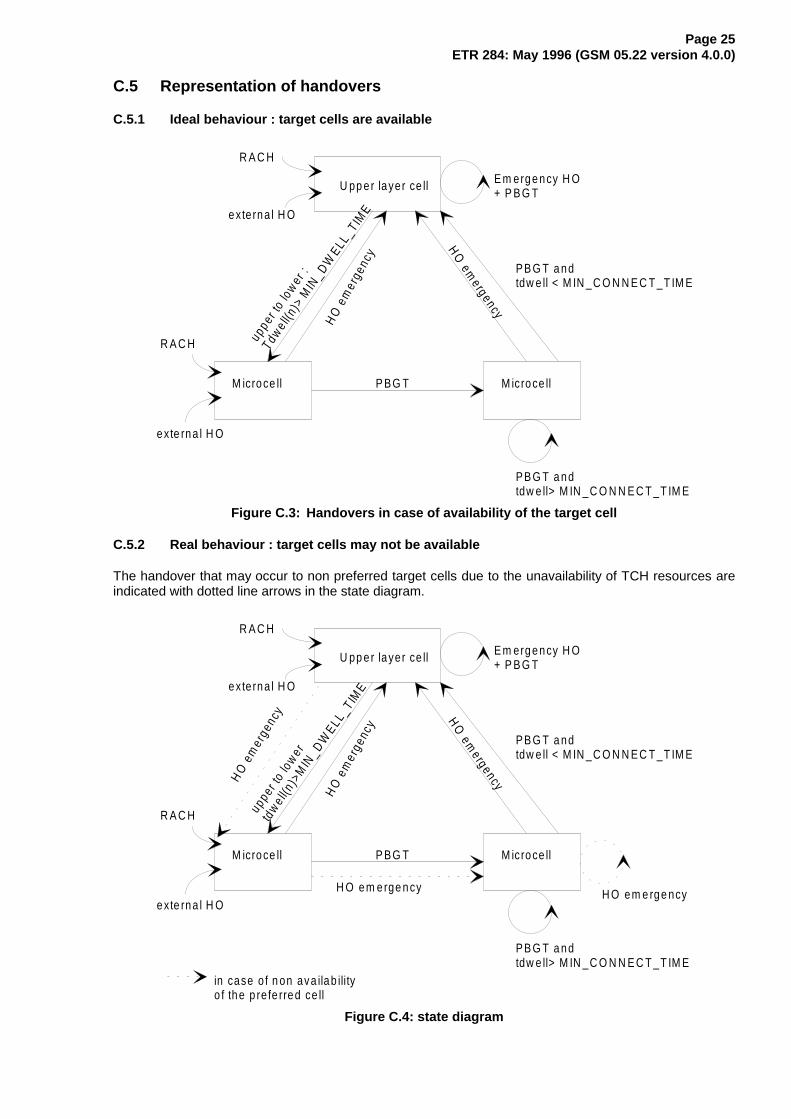
C.5.1 Ideal behaviour : target cells are available
U pp er layer ce ll
M icroce ll M icroce ll
R A C H
R A C H
externa l H O
exte rna l H O
E m ergency H O+ P B G T
uppe
r to
low
er :
T dwe l
l(n)>
MIN
_DW
ELL_T IM
E
HO
emerg ency
PB G T a ndtdw e ll> M IN _C O N N E C T _T IM E
P BG T
PB G T a nd tdw e ll < M IN _C O N N E C T _T IM E
HO
em
e rge
ncy
Figure C.3: Handovers in case of availability of the target cell
C.5.2 Real behaviour : target cells may not be available
The handover that may occur to non preferred target cells due to the unavailability of TCH resources areindicated with dotted line arrows in the state diagram.
U pp e r layer ce ll
M icroce ll M icroce ll
R A C H
R A C H
externa l H O
exte rna l H O
E m ergency H O+ P B G T
uppe
r to
low
er
tdw
e ll(n
)>M
IN_D
WELL
_TIM
E
HO
emerg ency
PB G T a ndtdw e ll> M IN _C O N N E C T _T IM E
P BG T
PB G T a nd tdw e ll < M IN _C O N N E C T _T IM E
HO
em
e rge
ncy
H O em erge ncy H O em e rge ncy
HO
em
erge
n cy
in case o f n on ava ilab ilityo f the p re fe rred ce ll
Figure C.4: state diagram
Page 26ETR 284: May 1996 (GSM 05.22 version 4.0.0)
C.6 Emergency handover
C.6.1 Target cell = upper layer cell
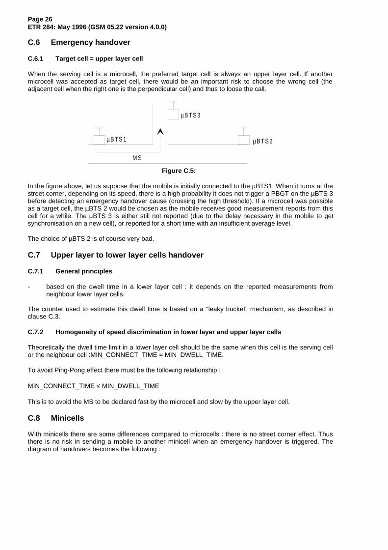
When the serving cell is a microcell, the preferred target cell is always an upper layer cell. If anothermicrocell was accepted as target cell, there would be an important risk to choose the wrong cell (theadjacent cell when the right one is the perpendicular cell) and thus to loose the call.
µ BT S 1 µ B T S 2
µ B T S 3
M S
Figure C.5:
In the figure above, let us suppose that the mobile is initially connected to the µBTS1. When it turns at thestreet corner, depending on its speed, there is a high probability it does not trigger a PBGT on the µBTS 3before detecting an emergency handover cause (crossing the high threshold). If a microcell was possibleas a target cell, the µBTS 2 would be chosen as the mobile receives good measurement reports from thiscell for a while. The µBTS 3 is either still not reported (due to the delay necessary in the mobile to getsynchronisation on a new cell), or reported for a short time with an insufficient average level.
The choice of µBTS 2 is of course very bad.
C.7 Upper layer to lower layer cells handover
C.7.1 General principles
- based on the dwell time in a lower layer cell : it depends on the reported measurements fromneighbour lower layer cells.
The counter used to estimate this dwell time is based on a "leaky bucket" mechanism, as described inclause C.3.
C.7.2 Homogeneity of speed discrimination in lower layer and upper layer cells
Theoretically the dwell time limit in a lower layer cell should be the same when this cell is the serving cellor the neighbour cell :MIN_CONNECT_TIME = MIN_DWELL_TIME.
To avoid Ping-Pong effect there must be the following relationship :
MIN_CONNECT_TIME ≤ MIN_DWELL_TIME
This is to avoid the MS to be declared fast by the microcell and slow by the upper layer cell.
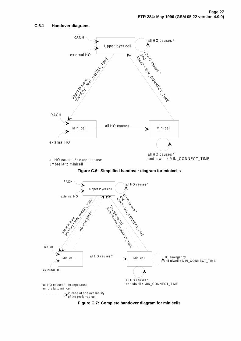
C.8 Minicells
With minicells there are some differences compared to microcells : there is no street corner effect. Thusthere is no risk in sending a mobile to another minicell when an emergency handover is triggered. Thediagram of handovers becomes the following :
Page 27ETR 284: May 1996 (GSM 05.22 version 4.0.0)
C.8.1 Handover diagrams
U pper la yer ce ll
M in i ce ll
R A C H
R A C H
ex te rna l H O
exte rna l H O
uppe
r to
low
er
tdw
e ll(n
) > M
IN_D
WELL
_TIM
E
a ll H O causes * M in i ce ll
a ll H O cau ses *and tdw e ll > M IN _C O N N E C T _T IM E
all HO
cause s *
a nd
tdwell < M
IN_C
ON
NEC
T_ TIME
a ll H O cau ses *
a ll H O ca use s * : except cause um b re lla to m in ice ll
Figure C.6: Simplified handover diagram for minicells
U pper la yer ce ll
M in i cell
RAC H
R ACH
exte rna l H O
ex te rn al H O
uppe
r to
low
e r
tdw
ell(n
) > M
IN_D
WELL
_TIM
E
a ll H O causes * M in i ce ll
a ll H O cau ses *and tdw e ll > M IN _C O N N EC T _T IM E
all HO
causes *
and
tdwell < M
IN_C
ON
NEC
T_TIME
a ll H O cau ses *
a ll H O ca uses * : except cause um b re lla to m in ice ll
HO
em
erge
ncy
H O em ergencya nd tdw e ll < M IN _C O N N EC T_ TIM E
Em
ergency HO
& tdwell>M
IN_C
ON
NEC
T_TIME
in case o f non ava ila bilityo f the p re fe rred ce ll
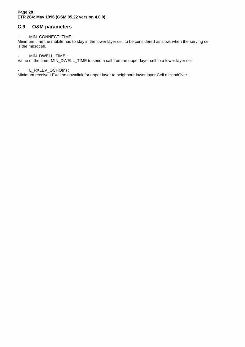
Figure C.7: Complete handover diagram for minicells
Page 28ETR 284: May 1996 (GSM 05.22 version 4.0.0)
C.9 O&M parameters
- MIN_CONNECT_TIME :Minimum time the mobile has to stay in the lower layer cell to be considered as slow, when the serving cellis the microcell.
- MIN_DWELL_TIME :Value of the timer MIN_DWELL_TIME to send a call from an upper layer cell to a lower layer cell.
- L_RXLEV_OCHO(n) :Minimum receive LEVel on downlink for upper layer to neighbour lower layer Cell n HandOver.
Page 29ETR 284: May 1996 (GSM 05.22 version 4.0.0)
Annex D: Example 4 (France Telecom/CNET)
Description of algorithm
Source : France Telecom/CNET
Date : 22.06.95
Subject : Informative Annex for high speed MS
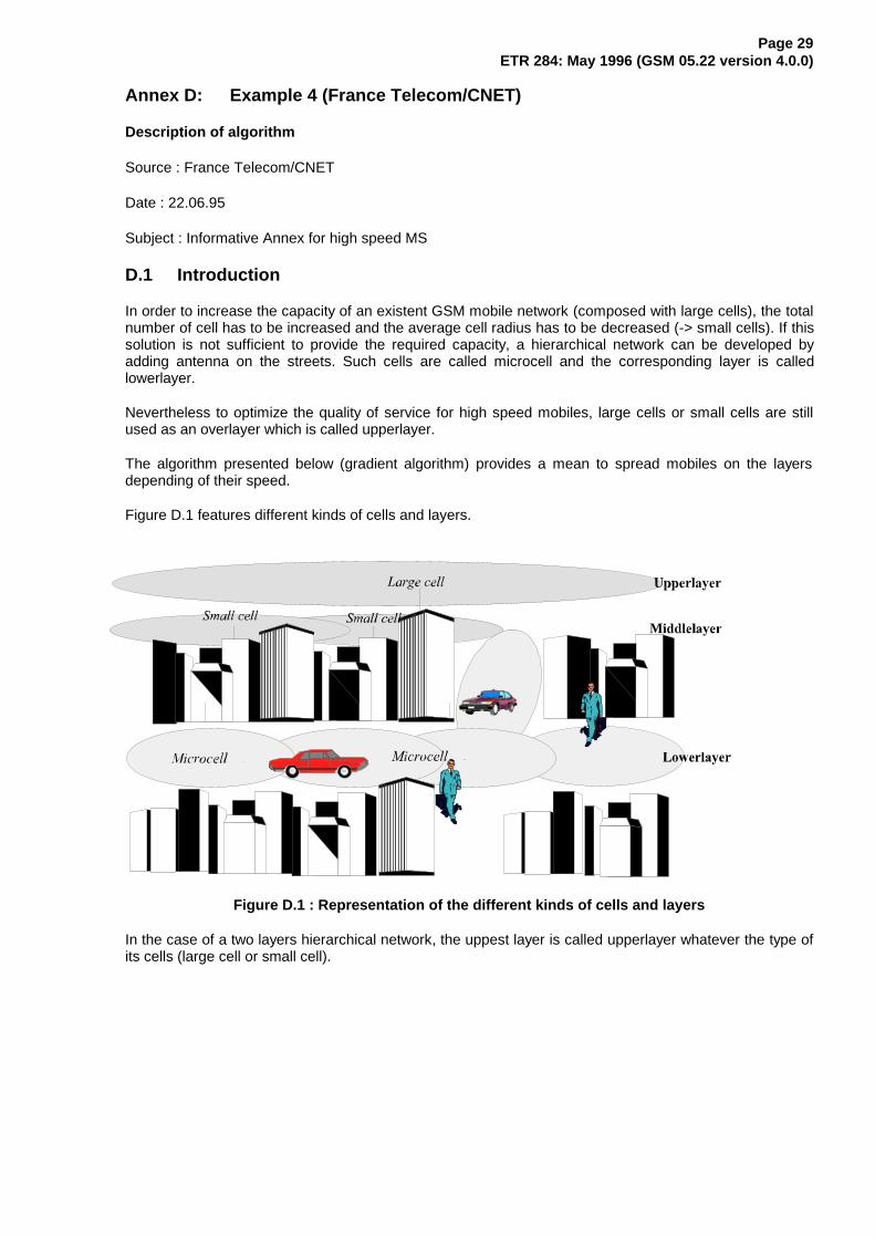
D.1 Introduction
In order to increase the capacity of an existent GSM mobile network (composed with large cells), the totalnumber of cell has to be increased and the average cell radius has to be decreased (-> small cells). If thissolution is not sufficient to provide the required capacity, a hierarchical network can be developed byadding antenna on the streets. Such cells are called microcell and the corresponding layer is calledlowerlayer.
Nevertheless to optimize the quality of service for high speed mobiles, large cells or small cells are stillused as an overlayer which is called upperlayer.
The algorithm presented below (gradient algorithm) provides a mean to spread mobiles on the layersdepending of their speed.
Figure D.1 features different kinds of cells and layers.
Figure D.1 : Representation of the different kinds of cells and layers
In the case of a two layers hierarchical network, the uppest layer is called upperlayer whatever the type ofits cells (large cell or small cell).
Page 30ETR 284: May 1996 (GSM 05.22 version 4.0.0)
D.2 Descriptions of the algorithm
Mobile speed is estimated from the variation of the field strength received by the mobile from the targetcell.
This method of estimation is based on the computation of the gradient between two averages of the fieldstrength received by the mobile from the target cell (see subclause D.4.1 Estimation of the field strengthvariations). This algorithm can be used in any kind of multicellular network (composed with two layers oremore than two layers).
Considering the case of a network composed with three layers.
A "fast" mobile connected to a cell of the lowerlayer must handover towards a cell of the middlelayer.Nevertheless the field strength received from the cell of the middlelayer must be high enough to trigger thehandover.
A "slow" mobile connected to the lowerlayer must handover towards a cell of the same layer.
In both cases the estimation of mobile speeds are based on the field strength received from a cell of thelowerlayer.
A "fast" mobile connected to a cell of the upperlayer must handover towards a cell of the same layer.
A "slow" mobile connected to a cell of the upperlayer must handover to a cell of the middlelayer. In bothcases the estimation of mobile speeds are based on the field strength received from a cell of themiddlelayer.
A "fast" mobile connected to a cell of the middlelayer must handover towards a cell of the upperlayer.Nevertheless the field strength received from the cell of the upperlayer must be high enough to trigger thehandover.
The estimation of mobile speeds are based on the field strength received from a cell of the middlelayer.
A "slow" mobile connected to a cell of the middlelayer must handover towards a cell of the lowerlayer. Theestimation of mobile speeds are based on the field strength received from a cell of the lowerlayer
D.3 Handover causes
Some causes trigger emergency handovers, others trigger computations of the estimation of the mobilespeed.
D.3.1 emergency handover causes
An emergency handover is performed as soon as the quality of service become too low (RXQUAL andRXLEV causes), the handover has to be fast and secured. Target cells are ordinated depending on thevalue of PBGT(n), nevertheless cells of the directly upper layer have priority.
ex : in a hierarchical network composed with two layers, emergency handovers in cells of the lowerlayerare performed in priority towards cells of the upperlayer.
a) Comparison of RXLEV_XX with L_RXLEV_XX_H (XX = DL or UL)
RXLEV_XX < L_RXLEV_HH_H
b) Comparison of RXQUAL_XX with L_RXQUAL_XX_H (XX = DL or UL)
RXQUAL_XX > L_RXQUAL_XX_H
Page 31ETR 284: May 1996 (GSM 05.22 version 4.0.0)
D.3.2 mobile speeds estimation causes
Mobile speeds are estimated as soon as a non emergency handover is required. Two handover causes,whom depend of the target cell type, provide a computation of the estimation of mobile speeds.
A PBGT criteria is used in the case of a target cell of the same layer as the source one.
A CATCH criteria is used in the case of a target cell of a lower layer than the source one.
The PBGT(n) criteria if defined as in the appendix A of recommendation GSM 05.08 [3] i.e. :
1) RXLEV_NCELL(n) > RXLEV_MIN(n) + Max(0,Pa)
where Pa = (MS_TXPWR_MAX(n) -P)
2) PBGT(n) - HO_MARGIN(n1,n2) > 0
where n1 : source celln2 : target cell
The CATCH criteria is defined as follow :
RXLEV_NCELL(0,n) > CATCH(0,n)
where RXLEV_NCELL(0,n) : RXLEV assessed on the BCCH carrier of the cell nCATCH(0,n) : field strength threshold
This comparison enables handover to be performed towards a cell of a lower layer whom received fieldstrength is considered to be high enough.
D.4 Mobile speeds estimations
As soon as one of the two causes described above is triggered (PBGT, CATCH) a process of computationof the estimation of the mobile speed is performed.
The method of estimation of the field strength variations is based on the computation of the gradientbetween two averages of field strengths received by the mobile from the target cell.
D.4.1 Estimation of the field strength variations
The first of the two averages of field strength used in the gradient computation is the one computed frommeasurements received from the target cell which has verified the handover criteria.
The handover cause can be either a PBGT or a CATCH one (see subclause D.3.2 mobile speedsestimation causes).
The second of the two field strength averages used in the gradient computation is the latest one for whichthe gaps between all the previous averages and the straight line passing-by the two averages definedabove is lower than Emax (E < Emax) .
Emax is one of the parameters of the handover algorithm.
The gradient is then computed as follow :
1) GRAD = ((RXLEV_NCELL(n,No) - RXLEV_NCELL(n,No-m))/mwhere:- n is the respective adjacent cell "n"- No is the index of reference of the average for which the handover criteria has been verified- m is the last average for which E < Emax- RXLEV_NCELL(0,n) is the RXLEV assessed on the BCCH carrier of the cell n
Page 32ETR 284: May 1996 (GSM 05.22 version 4.0.0)
In order to ensure an efficiency estimation of the mobile speeds a minimum number of averages (NAmin)are necessary to trigger the computation of the gradient.
To avoid high computed time and high memory size a maximum number of averages (NAmax) has to bekept.
The number of averages to take into account shall verified the following condition :
2) NAmin < N < NAmaxwhere:- NAmin is the minimum number of averages necessary to compute the gradient- NAmax is the maximum number of averages necessary to compute the gradient
If the number of averages is not high enough (N < NAmin) a default handover algorithm is used.
The handover towards an upper layer is performed only if the above conditions are verified and if the fieldstrength received from the target cell verified the following condition :
3) RXLEV > U_RXLEV_NCELL(0,n)where:- -U_RXLEV_NCELL(0,n) is the minimum field strength assessed from the BCCH carrier of
the upper layer target cell to performed a handover towards it.
D.5 BSS decision algorithm :
The BSS decision algorithm is the classical one as described in the appendix A of the recommendationGSM 05.08 [3]. Nevertheless in the case of an emergency handover, cells of the directly upper layer haspriority. If no cell of the directly upper layer is available, cells of the same layer are ordering depending ofthe PBGT(n2) - HO_MARGIN(n1,n2) values.
D.6 O&M parameters
CELL_TYPE : Hierarchy level of serving cellRange 0-7Step size 1Coding 0 : microcell
1 : small cell2 : large cell3-7 : for future use
NCELL_TYPE(n) : Hierarchy level of n-th neighbour celln 1-32Range 0-7Step size 1Coding 0 : microcell
1 : small cell2 : large cell3-7 : for future use
EN_MS_SPEED : Enable/Disable classification of MS regarding SPEEDCoding 0 : disable feature
1 : enable feature
NAmax : Maximum number of averages necessary to compute the gradient.Range 0 - 63 (SACCH)Step size 1
NAmin : Minimum number of averages necessary to compute the gradient.Range 0 - 63 (SACCH)Step size 1
Page 33ETR 284: May 1996 (GSM 05.22 version 4.0.0)
Emax : Maximum gap allowed between a computed average and the straight line considered.Range 0 - 15 (dB)Step size 1
GRAD : Gradient threshold. It depends of the mobile speed threshold. Middlelayers have two Grad thresholds (Gradmin & Gradmax), the upperlayer and the lowerlayer has one threshold (Grad).Range 0 - 255Step size 1
CATCH(n) : Minimum field strength threshold. This is the minimum field strength the mobile has to receive from a cell of the directly lower layer to perform a handover.Range 0 - 63 (dB)Step size 1
U_RXLEV_NCELL(0,n): Field strength threshold. This is the minimum field strength necessary to receive from the upper layer cell to performed a handover towards it.Range 0 - 63Step size 1
D.7 Examples
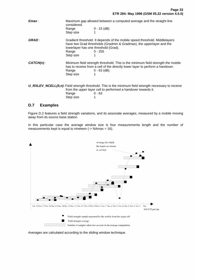
Figure D.2 features a field strength variations, and its associate averages, measured by a mobile movingaway from its source base station.
In this particular case the average window size is four measurements length and the number ofmeasurements kept is equal to nineteen (-> NAmax = 16).
Averages are calculated according to the sliding window technique.
Page 34ETR 284: May 1996 (GSM 05.22 version 4.0.0)
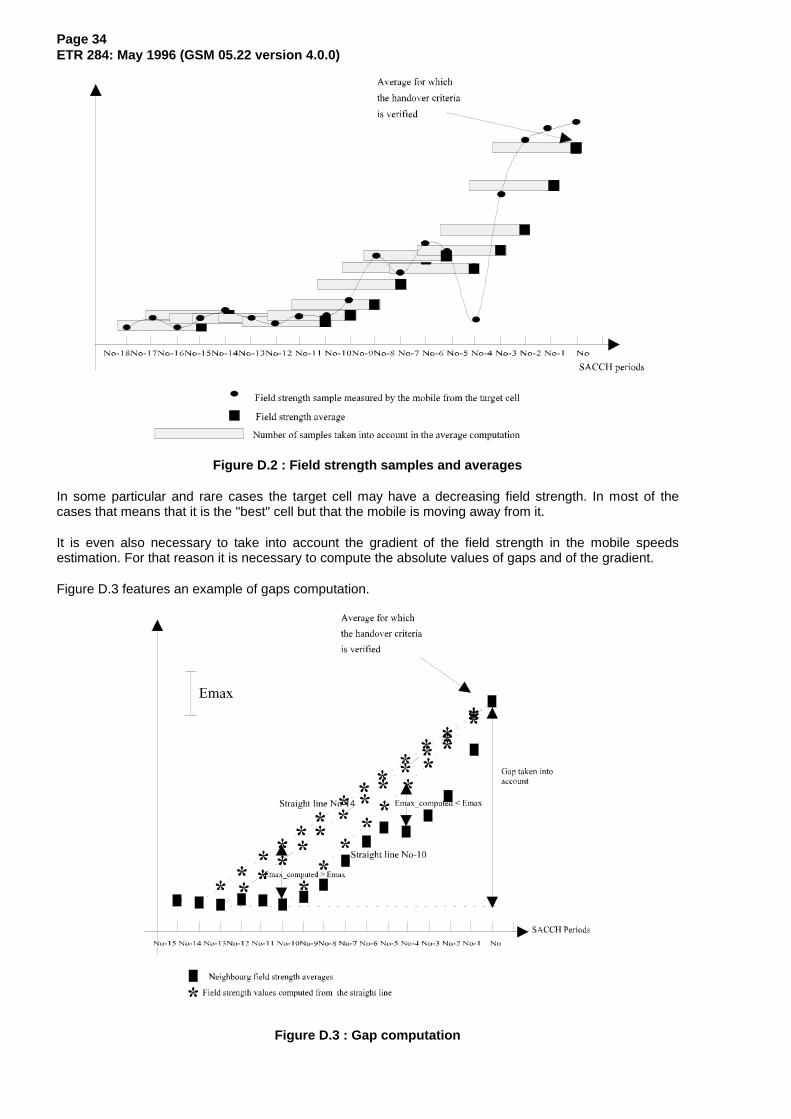
Figure D.2 : Field strength samples and averages
In some particular and rare cases the target cell may have a decreasing field strength. In most of thecases that means that it is the "best" cell but that the mobile is moving away from it.
It is even also necessary to take into account the gradient of the field strength in the mobile speedsestimation. For that reason it is necessary to compute the absolute values of gaps and of the gradient.
Figure D.3 features an example of gaps computation.
Figure D.3 : Gap computation
Page 35ETR 284: May 1996 (GSM 05.22 version 4.0.0)
For each average computed (n), from the latest to the oldest, the algorithm determines the maximum gapwith the corresponding field strength computed from the straight line (*).
Considering the average computed at date N0-10 in the particular case of figure D.3. The maximum gapcomputed Emax_computed , between the nine previous averages (from N0-1 to N0-9) and the straightline N0-10, is lower than the maximum gap allowed Emax .
On the other hand considering the average computed at date N0-14. The gap computed between theaverage on date N0-10 and the straight line N0-14 is higher than the maximum gap allowed Emax.
In this case the last average for which the maximum gap computed is lower than Emax is the onecomputed on date N0-13.
In this case the gradient of the field strength is equal to :
GRAD = (RXLEV_NCELL(n,No) - RXLEV_NCELL(n,No-13))/13
where :
RXLEV_NCELL(n,N 0) : RXLEV assessed on the BCCH carrier of the cell n, which has verified thehandover criteria (date N0).
RXLEV_NCELL(n,N 0-13) : RXLEV assessed on the BCCH carrier of the cell, computed on date N0-13.
In the case of figure D.3, averages are almost constants from date N0-10 to N0-15, it can be the case forexample for a mobile stopped at a traffic light . The parameter Emax avoid to take into account theseaverages in the estimation of the mobile speeds.
D.8 State diagrams
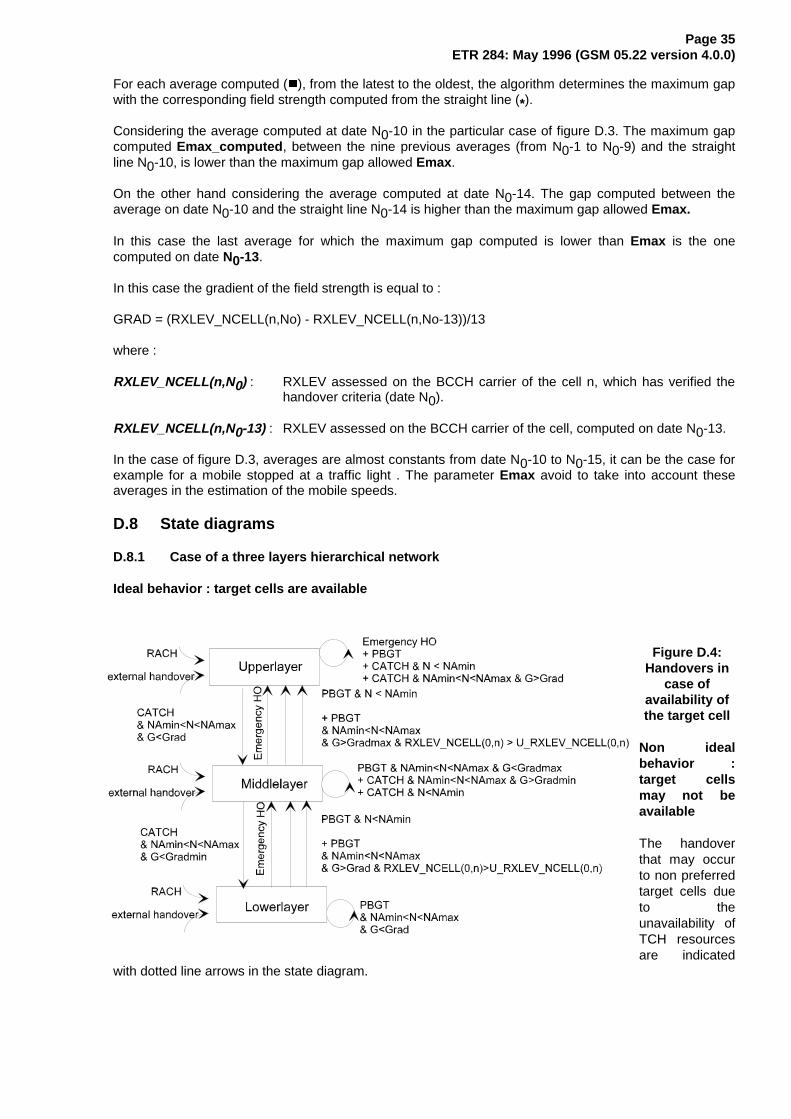
D.8.1 Case of a three layers hierarchical network
Ideal behavior : target cells are available
Figure D.4:Handovers in
case ofavailability ofthe target cell
Non idealbehavior :target cellsmay not beavailable
The handoverthat may occurto non preferredtarget cells dueto theunavailability ofTCH resourcesare indicated
with dotted line arrows in the state diagram.
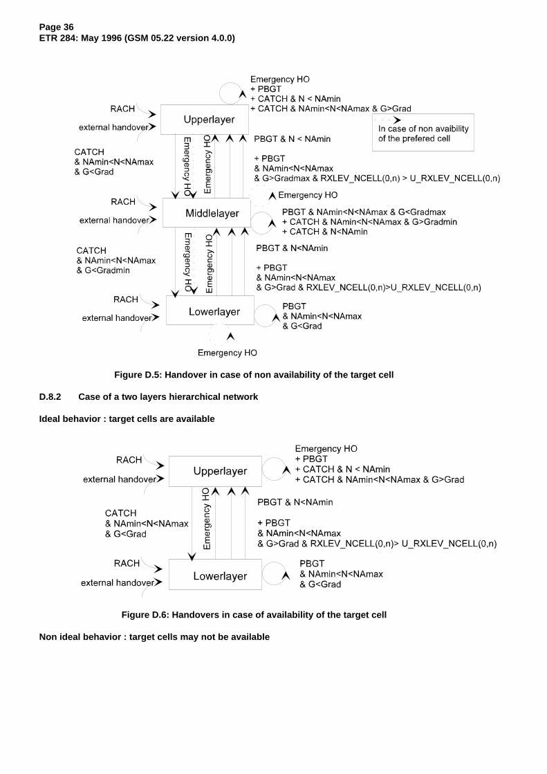
Page 36ETR 284: May 1996 (GSM 05.22 version 4.0.0)
Figure D.5: Handover in case of non availability of the target cell
D.8.2 Case of a two layers hierarchical network
Ideal behavior : target cells are available
Figure D.6: Handovers in case of availability of the target cell
Non ideal behavior : target cells may not be available

Page 37ETR 284: May 1996 (GSM 05.22 version 4.0.0)
The handover that may occur to non preferred target cells due to the unavailability of TCH resources areindicated with dotted line arrows in the state diagram.
Figure D.7: Handover in case of non availability of the target cell
Page 38ETR 284: May 1996 (GSM 05.22 version 4.0.0)
Annex E: Simulation Model for Handover Performance Evaluation inHierarchical Cell Structures
E.1 Introduction
In this Annex, the general requirements of a simulation model for handover performance evaluation inhierarchical cell structures are specified.
The following criteria are considered fundamental for the design of the overall simulation model:
- Mobile environment- Radio network model- Propagation model- Motion model- Handover algorithms- Measurement reporting- Performance criteria.
E.2 Mobile Environment
The single mobile environment is taken to allow relatively simple simulations and easier interpretation ofthe performance results.
In order to simulate the interference that may occur, a detailed frequency allocation pattern and a largenumber of cells are required. In the single mobile environment, the interference situation is not taken intoaccount. Therefore, handovers due to quality are not simulated. However, this enables the very evaluationof the handover algorithm, and not the evaluation of the frequency pattern.
E.3 Radio Network Model
The radio network model represents the network layout. It should allow the definition of the followingparameters:
- Number of layers- Number of cells on each layer- BTS site pattern- BTS separation
Three network model scenarios are proposed.
E.3.1 Scenario 1: Hot Spot
One cell in the upper layer, one cell in the lower layer.
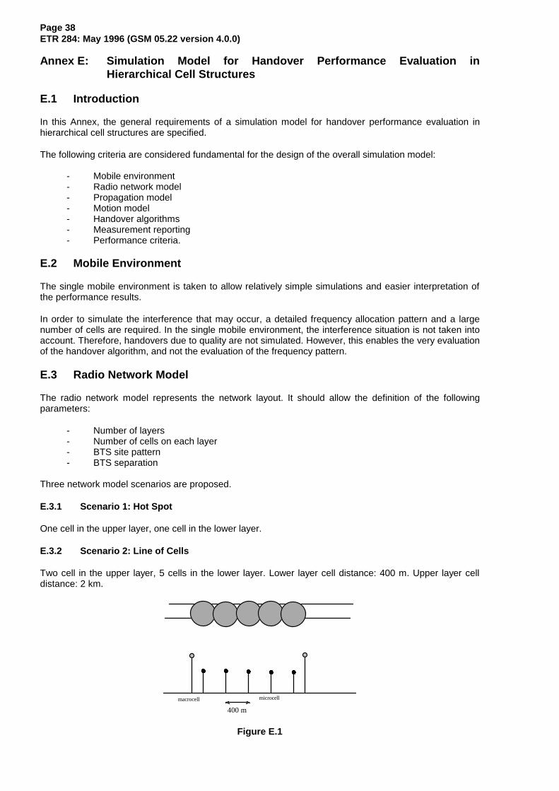
E.3.2 Scenario 2: Line of Cells
Two cell in the upper layer, 5 cells in the lower layer. Lower layer cell distance: 400 m. Upper layer celldistance: 2 km.
lllll
400 m
macrocell microcell
Figure E.1
Page 39ETR 284: May 1996 (GSM 05.22 version 4.0.0)
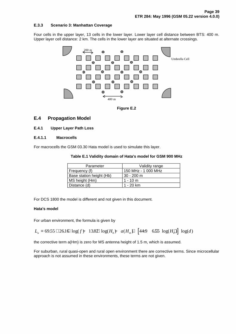
E.3.3 Scenario 3: Manhattan Coverage
Four cells in the upper layer, 13 cells in the lower layer. Lower layer cell distance between BTS: 400 m.Upper layer cell distance: 2 km. The cells in the lower layer are situated at alternate crossings.
Umbrella Cell
200 m
400 m
Figure E.2
E.4 Propagation Model
E.4.1 Upper Layer Path Loss
E.4.1.1 Macrocells
For macrocells the GSM 03.30 Hata model is used to simulate this layer.
Table E.1 Validity domain of Hata's model for GSM 900 MHz
Parameter Validity rangeFrequency (f) 150 MHz - 1 000 MHzBase station height (Hb) 30 - 200 mMS height (Hm) 1 - 10 mDistance (d) 1 - 20 km
For DCS 1800 the model is different and not given in this document.
Hata's model
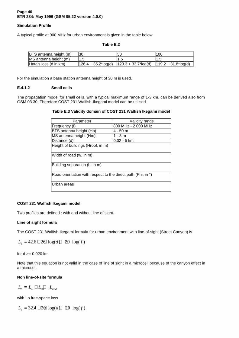
For urban environment, the formula is given by
[ ]L f H a H H du b m b= + ⋅ − ⋅ − + − ⋅ ⋅69 55 2616 1382 44 9 655. . log( ) . log( ) ( ) . . log( ) log( )
the corrective term a(Hm) is zero for MS antenna height of 1.5 m, which is assumed.
For suburban, rural quasi-open and rural open environment there are corrective terms. Since microcellularapproach is not assumed in these environments, these terms are not given.
Page 40ETR 284: May 1996 (GSM 05.22 version 4.0.0)
Simulation Profile
A typical profile at 900 MHz for urban environment is given in the table below
Table E.2
BTS antenna height (m) 30 50 100MS antenna height (m) 1.5 1.5 1.5Hata's loss (d in km) 126.4 + 35.2*log(d) 123.3 + 33.7*log(d) 119.2 + 31.8*log(d)
For the simulation a base station antenna height of 30 m is used.
E.4.1.2 Small cells
The propagation model for small cells, with a typical maximum range of 1-3 km, can be derived also fromGSM 03.30. Therefore COST 231 Walfish-Ikegami model can be utilised.
Table E.3 Validity domain of COST 231 Walfish Ikegami model
Parameter Validity rangeFrequency (f) 800 MHz - 2 000 MHzBTS antenna height (Hb) 4 - 50 mMS antenna height (Hm) 1 - 3 mDistance (d) 0.02 - 5 kmHeight of buildings (Hroof, in m)
Width of road (w, in m)
Building separation (b, in m)
Road orientation with respect to the direct path (Phi, in °)
Urban areas
COST 231 Walfish Ikegami model
Two profiles are defined : with and without line of sight.
Line of sight formula
The COST 231 Walfish-Ikegami formula for urban environment with line-of-sight (Street Canyon) is
L d fb = + ⋅ + ⋅42 6 26 20. log( ) log( )
for d >= 0.020 km
Note that this equation is not valid in the case of line of sight in a microcell because of the canyon effect ina microcell.
Non line-of-site formula
L L L Lb o rts msd= + +
with Lo free-space loss
L d fo = + ⋅ + ⋅32 4 20 20. log( ) log( )
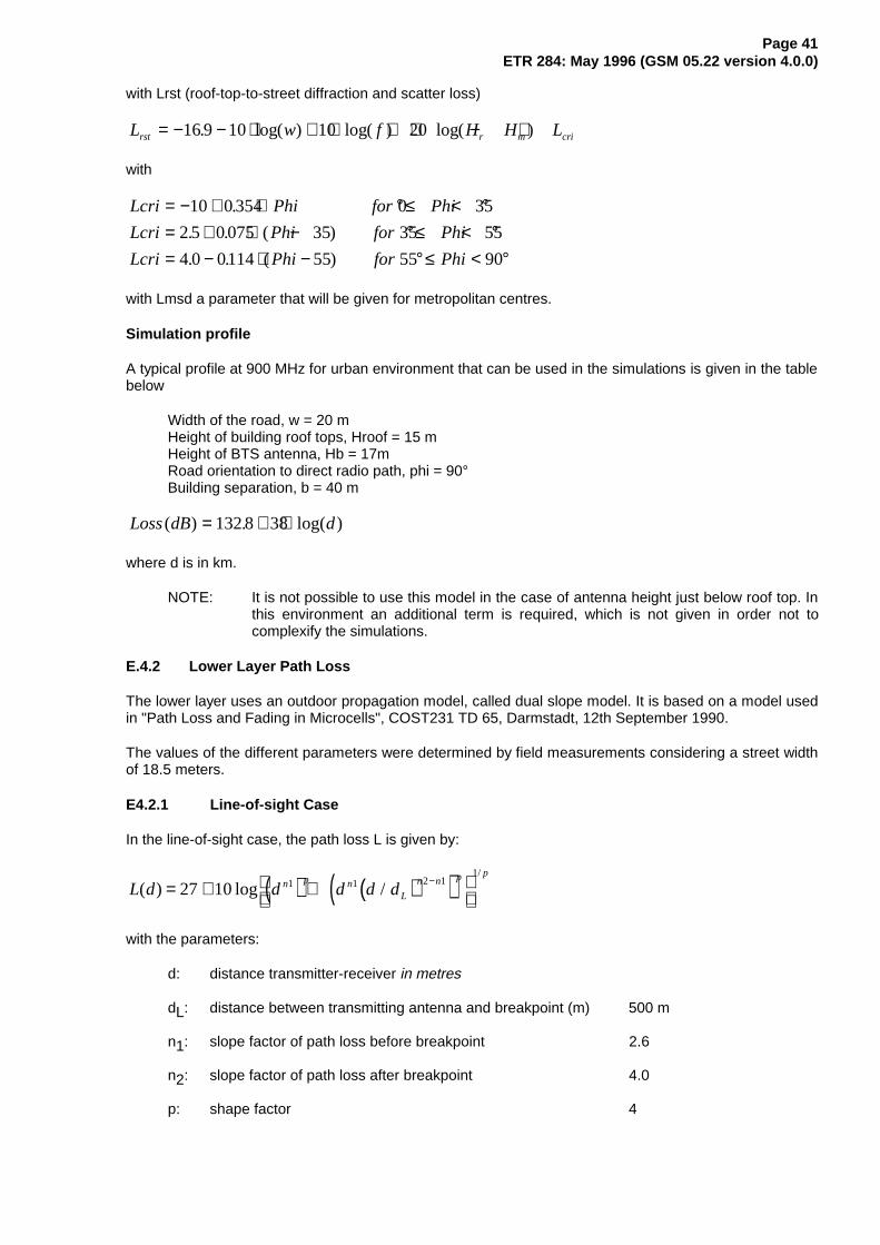
Page 41ETR 284: May 1996 (GSM 05.22 version 4.0.0)
with Lrst (roof-top-to-street diffraction and scatter loss)
L w f H H Lrst r m cri= − − ⋅ + ⋅ + ⋅ − +16 9 10 10 20. log( ) log( ) log( )
with
Lcri Phi for Phi
Lcri Phi for Phi
Lcri Phi for Phi
= − + ⋅ °≤ < °= + ⋅ − °≤ < °= − ⋅ − °≤ < °
10 0 354 0 35
2 5 0 075 35 35 55
4 0 0114 55 55 90
.
. . ( )
. . ( )
with Lmsd a parameter that will be given for metropolitan centres.
Simulation profile
A typical profile at 900 MHz for urban environment that can be used in the simulations is given in the tablebelow
Width of the road, w = 20 mHeight of building roof tops, Hroof = 15 mHeight of BTS antenna, Hb = 17mRoad orientation to direct radio path, phi = 90°Building separation, b = 40 m
Loss dB d( ) . log( )= + ⋅132 8 38
where d is in km.
NOTE: It is not possible to use this model in the case of antenna height just below roof top. Inthis environment an additional term is required, which is not given in order not tocomplexify the simulations.
E.4.2 Lower Layer Path Loss
The lower layer uses an outdoor propagation model, called dual slope model. It is based on a model usedin "Path Loss and Fading in Microcells", COST231 TD 65, Darmstadt, 12th September 1990.
The values of the different parameters were determined by field measurements considering a street widthof 18.5 meters.
E4.2.1 Line-of-sight Case
In the line-of-sight case, the path loss L is given by:
( ) ( )( )L d d d d dn p nL
n n p p
( ) log //
= + +
−27 10 1 1 2 1
1
with the parameters:
d: distance transmitter-receiver in metres
dL: distance between transmitting antenna and breakpoint (m) 500 m
n1: slope factor of path loss before breakpoint 2.6
n2: slope factor of path loss after breakpoint 4.0
p: shape factor 4
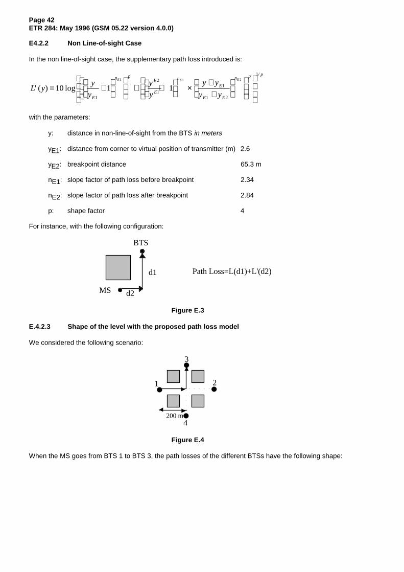
Page 42ETR 284: May 1996 (GSM 05.22 version 4.0.0)
E4.2.2 Non Line-of-sight Case
In the non line-of-sight case, the supplementary path loss introduced is:
L yy
y
y
y
y y
y yE
n pE
E
n
E
E E
n p pE E E
' ( ) log
/
= +
+ +
×
++
10 1 11
2
11
1 2
11 1 2
with the parameters:
y: distance in non-line-of-sight from the BTS in meters
yE1: distance from corner to virtual position of transmitter (m) 2.6
yE2: breakpoint distance 65.3 m
nE1: slope factor of path loss before breakpoint 2.34
nE2: slope factor of path loss after breakpoint 2.84
p: shape factor 4
For instance, with the following configuration:
BTS
MS
d1
d2
Path Loss=L(d1)+L'(d2)
Figure E.3
E.4.2.3 Shape of the level with the proposed path loss model
We considered the following scenario:
1 2
3
4200 m
Figure E.4
When the MS goes from BTS 1 to BTS 3, the path losses of the different BTSs have the following shape:
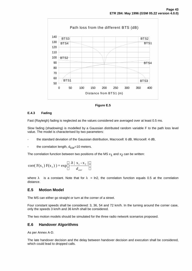
Page 43ETR 284: May 1996 (GSM 05.22 version 4.0.0)
Path loss f rom the dif ferent B T S (dB )
Dis tance from B T S 1 (m)
5060
70
80
90
100
110
120130
140
0 50 100 150 200 250 300 350 400
BT S 1
BT S 2
BT S 3BT S 4 BT S 1
BT S 2
BT S 3
BT S 4
Figure E.5
E.4.3 Fading
Fast (Rayleigh) fading is neglected as the values considered are averaged over at least 0.5 ms.
Slow fading (shadowing) is modelled by a Gaussian distributed random variable F to the path loss levelvalue. The model is characterised by two parameters:
- the standard deviation of the Gaussian distribution, Macrocell: 6 dB, Microcell: 4 dB,
- the correlation length, dcor=10 meters.
The correlation function between two positions of the MS x1 and x2 can be written:
corr( F(x ) F(x ) ) = exp - | x - x |
1 21 2λ
dcorr
where λ is a constant. Note that for λ = ln2, the correlation function equals 0.5 at the correlationdistance.
E.5 Motion Model
The MS can either go straight or turn at the corner of a street.
Four constant speeds shall be considered: 3, 36, 54 and 72 km/h. In the turning around the corner case,only the speeds 3 km/h and 36 km/h shall be considered.
The two motion models should be simulated for the three radio network scenarios proposed.
E.6 Handover Algorithms
As per Annex A-D.
The late handover decision and the delay between handover decision and execution shall be considered,which could lead to dropped calls.
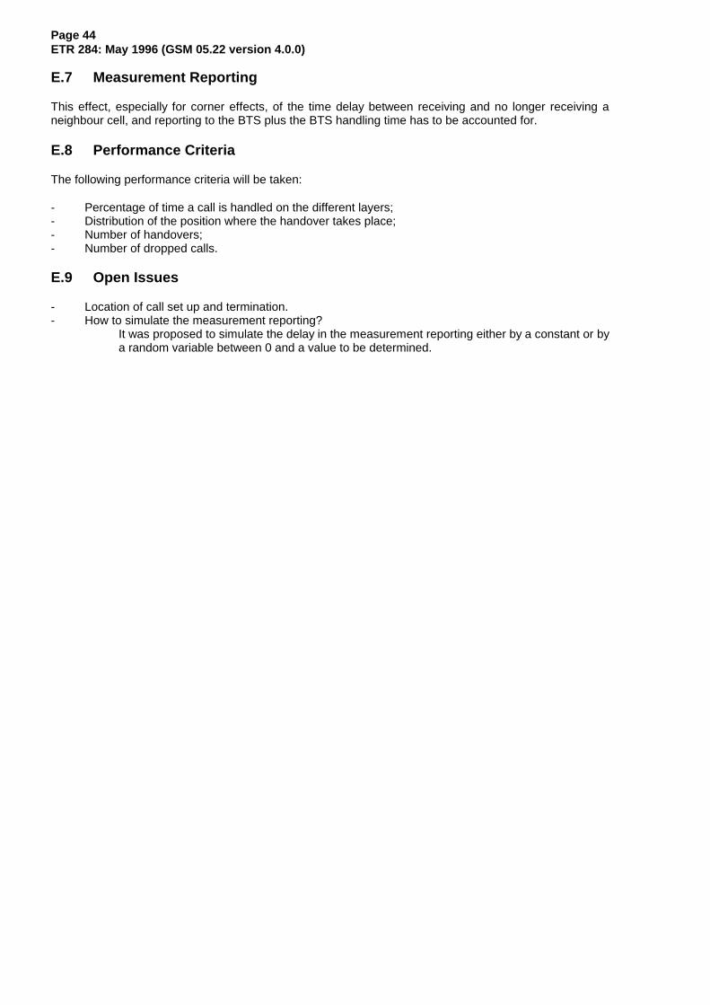
Page 44ETR 284: May 1996 (GSM 05.22 version 4.0.0)
E.7 Measurement Reporting
This effect, especially for corner effects, of the time delay between receiving and no longer receiving aneighbour cell, and reporting to the BTS plus the BTS handling time has to be accounted for.
E.8 Performance Criteria
The following performance criteria will be taken:
- Percentage of time a call is handled on the different layers;- Distribution of the position where the handover takes place;- Number of handovers;- Number of dropped calls.
E.9 Open Issues
- Location of call set up and termination.- How to simulate the measurement reporting?
It was proposed to simulate the delay in the measurement reporting either by a constant or bya random variable between 0 and a value to be determined.
Page 45ETR 284: May 1996 (GSM 05.22 version 4.0.0)
History
Document history
May 1996 First Edition
ISBN 2-7437-0698-8Dépôt légal : Mai 1996