Embed Size (px)
Citation preview
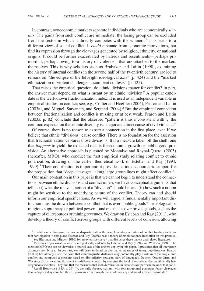
American Economic Review 2012, 102(4): 1310–1342 http://dx.doi.org/10.1257/aer.102.4.1310
1310
Ethnicity and Conflict: An Empirical Study†
By Joan Esteban, Laura Mayoral, and Debraj Ray*
We examine empirically the impact of ethnic divisions on conflict, by using a specification based on Esteban and Ray (2011). That theory links conflict intensity to three indices of ethnic distribution: polar-ization, fractionalization, and the Gini-Greenberg index. The empiri-cal analysis verifies that these distributional measures are significant correlates of conflict. These effects persist as we introduce country-specific measures of group cohesion and of the importance of public goods, and combine them with the distributional measures exactly as described by the theory. (JEL D63, D74, J15, O15, O17)
This paper examines the link between measures of ethnic distribution and social conflict.
The influence of the Marxian paradigm is clearly seen in the traditional view that income or wealth inequality is a major potential cause of conflict. Early empiri-cal studies emphasized indicators of income or wealth distribution as possible cor-relates of conflict (see, e.g., Brockett 1992; Midlarski 1988; Muller and Seligson 1987; Muller et al. 1989; and Nagel 1974, among several others). As the survey article by Lichbach (1989) concludes, however, the results obtained were generally ambiguous, or statistically insignificant.
The emphasis on inequality as a driver of conflict is natural, in the sense that the poor might be reasonably expected to harbor strong antagonisms against the rich. Yet the existence of antagonisms is only part of the story. The prevalence of sus-tained conflict requires those antagonisms to be channeled into organized action, often a tall order when economic strengths are so disparate. The clear economic demarcation across classes is a two-edged sword: while it breeds resentment, the very poverty of the have-nots militates against a successful insurrection, and even then the different skill and occupational niches occupied by capitalist and worker makes effective redistribution across classes a more indirect and difficult prospect.
* Esteban: Instituto de Análisis Económico (CSIC) and Barcelona GSE, 08193 Bellaterra, Barcelona, Spain (e-mail: [email protected]); Mayoral: CSIC and Barcelona GSE, 08193 Bellaterra, Barcelona, Spain (e-mail: [email protected]); Ray: Department of Economics, New York University, New York, NY 10012 (email: [email protected]). We gratefully acknowledge financial support from CICYT project ECO2011-25293 and Recercaixa. Esteban and Mayoral are beneficiaries of a financial contribution from the AXA Research Fund. Ray’s research was funded by National Science Foundation Grant SES-0962124 and a Fulbright-Nehru Fellowship from the Fulbright Foundation. He thanks the Indian Statistical Institute for warm hospitality during a year of leave from NYU. We are very grateful to James Fearon for giving us access to his dataset on ethnic groups, to Ignacio Ortuño-Ortín, who computed linguistic indices for us based on the Ethnologue dataset, and to Michael Ross for his dataset on natural resources. We are grateful to Oeindrila Dube, Kaivan Munshi, Natalija Novta, and Romain Wacziarg for helpful com-ments, to Laura Cozma, Andrew Gianou, and Bo ̌ r ek Vaší ̌ c ek for superb research assistance, and to seminar participants at various venues where this paper was presented. Finally, we acknowledge constructive comments by three anony-mous referees; the final version owes much to them.
† To view additional materials, visit the article page at http://dx.doi.org/10.1257/aer.102.4.1310.
ContentsEthnicity and Conflict: An Empirical Study† 1310
I. Theory 1313II. Empirical Implementation: Data and Conceptual Issues 1315A. Conflict 1315B. Distributional Indices 1316C. Additional Variables 1317III. Baseline Findings 1318A. Specification 1318B. Baseline 1318C. Country Examples and Scatters 1320IV. Extensions and Variations 1322A. Alternative Measures of Conflict 1322B. Alternative Groupings 1324C. Group Distances 1325D. Onset versus Incidence 1328E. Region and Time Effects 1328F. Alternative Estimation Strategies 1329V. Intercountry Variations in Publicness, Privateness, and Cohesion 1331VI. Summary and Conclusions 1335Appendix 1337REFERENCES 1340
1311EsTEBAn ET AL.: EThniciTy And confLicT: An EmpiRicAL sTudyVoL. 102 no. 4
In contrast, noneconomic markers separate individuals who are economically sim-ilar. The gains from such conflict are immediate: the losing group can be excluded from the sector in which it directly competes with the winners.1 This leads to a different view of social conflict. It could emanate from economic motivations, but find its expression through the cleavages generated by religion, ethnicity, or national origins. It could be further exacerbated by hatreds and resentments—perhaps pri-mordial, perhaps owing to a history of violence—that are attached to the markers themselves. This is why scholars such as Brubaker and Laitin (1998), examining the history of internal conflicts in the second half of the twentieth century, are led to remark on “the eclipse of the left-right ideological axis” (p. 424) and the “marked ethnicization of violent challenger-incumbent contests” (p. 425).
That raises the empirical question: do ethnic divisions matter for conflict? In part, the answer must depend on what is meant by an ethnic “division.” A popular candi-date is the well-known fractionalization index. It is used as an independent variable in empirical studies on conflict; see, e.g., Collier and Hoeffler (2004), Fearon and Laitin (2003a), and Miguel, Satyanath, and Sergenti (2004).2 But the empirical connection between fractionalization and conflict is missing or at best weak. Fearon and Laitin (2003a, p. 82) conclude that the observed “pattern is thus inconsistent with … the common expectation that ethnic diversity is a major and direct cause of civil violence.”
Of course, there is no reason to expect a connection in the first place, even if we believe that ethnic “divisions” cause conflict. There is no foundation for the assertion that fractionalization captures those divisions. It is a measure taken off the shelf, one that happens to yield the expected results for economic growth or public good pro-vision. An alternative approach is pursued by Montalvo and Reynal-Querol (2005) (hereafter, MRQ), who conduct the first empirical study relating conflict to ethnic polarization, drawing on the earlier theoretical work of Esteban and Ray (1994, 1999).3 Their contribution is important: it provides serious econometric support for the proposition that “deep cleavages” along large group lines might affect conflict.4
Our main contention in this paper is that we cannot begin to understand the connec-tions between ethnic divisions and conflict unless we have conceptual arguments that tell us (i) what the relevant notion of a “division” should be, and (ii) how such a notion might be sensitive to the underlying nature of the conflict. Theory can and should inform our empirical specifications. As we will argue, a fundamentally important dis-tinction must be drawn between a conflict that is over “public goods”—ideological or religious supremacy, or political power—and one that is over private goods, such as the capture of oil resources or mining revenues. We draw on Esteban and Ray (2011), who develop a theory of conflict across groups with different levels of cohesion, allowing
1 In addition, within-group economic disparities allow the complementary activities of conflict funding and con-flict participation to take place. Esteban and Ray (2008a) base a theory of ethnic salience in conflict on this premise.
2 See Blattman and Miguel (2010) for an extensive survey that discusses these papers and related literature.3 Measures of polarization were developed independently by Esteban and Ray (1994) and Wolfson (1994). The
measure MRQ use can be viewed as a special case of the one we deploy in this paper. It presumes that all intergroup distances are “binary.” In contrast, we will draw in detail on alternative measures of intergroup distances. Fearon (2003a) has already made the point that ethnolinguistic distances may potentially play a role in explaining ethnic conflict and computed a measure based on dissimilarity between pairs of languages. Desmet, Ortuño-Ortín, and Wacziarg (2012) examine this point in a different context, by studying the level of social transfers in ethnically het-erogeneous societies. They find that the measures that include variation in distances outperform the ones that don’t.
4 Recall Horowitz (1985, p. 39): “A centrally focused system [with few groupings] possesses fewer cleavages than a dispersed system, but those it possesses run through the whole society and are of greater magnitude.”
1312 ThE AmERicAn Economic REViEW JunE 2012
for such “public” and “private” prizes as well as different mixes of those prizes. We review their approach briefly in Section I. They show that the equilibrium intensity of conflict is linearly related to just three measures of distribution and no other: polariza-tion (p), fractionalization (f), and a Greenberg-Gini index of ethnic difference (G), all to be formally defined below (see Proposition 1). Moreover, the model tells us that the weight of each of these indices in explaining conflict intensity depends on the particu-lar nature of each conflict. Specifically, ethnic polarization will influence conflict if the prize is public and group cohesion is high, and ethnic fractionalization will influence conflict if the prize is private (and group cohesion, once again, is high). Finally, the Greenberg-Gini difference index becomes relatively important in explaining conflict if group cohesion is low.
The purpose of the current paper is to bring these theoretical predictions to the data. We study 138 countries over 1960–2008. We begin by implementing the idea that the equilibrium level of conflict is linked to the three distributional measures identified above. Across a variety of specifications and robustness checks (described in Tables 1–8), the ethnic polarization measure is highly significant and positive, the effect of fractionalization is equally large and positive, though somewhat less significant, and the Greenberg-Gini, while significant, affects conflict negatively. The fact that polarization is strongly significant suggests that disputes over public goods, broadly defined, is an important feature of social conflicts. Such public goods could be narrowly economic, such as access to a particular trade or a labor market, or they could represent political power or cultural dominance, or plain animosity. The fact that fractionalization is significant as well suggests that divisible pecuniary benefits also play a role in conflict. Finally, the importance of polarization and frac-tionalization, and the fact that G enters negatively, can together be interpreted, using the theory, as an indicator that within-group cohesion in the contribution of conflict resources is particularly high in situations of open conflict.
Recall that the relative importance of p and f in explaining conflict depends on the extent to which payoffs are public rather than private. The previous exercise implicitly assumes that this composition is the same across countries. In the remainder of the paper, we take the analysis a step forward by constructing proxies for country-specific values of relative publicness from ancillary data. To do so, we employ indicators for privateness or publicness of the prize that vary across countries. We capture private-ness by oil reserves, and publicness by different measures of autocracy (see Section V for more details). With these two sets of indicators we construct an index of relative publicness Λ. We use the structure of Proposition 1 to create the variables p × Λ and f × (1 − Λ). These variables test for the ideas that the impact of polarization is heightened by relative publicness Λ, while that of fractionalization is enhanced by relative privateness 1 − Λ. Our second main result is that these assertions (see the first three columns of Table 9) are supported to a remarkable degree.
In the foregoing analysis, we continued to assume that the level of within-group cohesion is the same across the countries in our sample. In a last step that exploits fully the structure of the theory, we use indicators from the World Values survey to estimate group cohesion by country, and then enter all these variables into the regres-sion exactly as specified by the model. This permits sharper tests that rely even more deeply on the structure of the model. Once again, we invoke Proposition 1 to inform the empirical specification, and once again our results are strongly supportive of the
1313EsTEBAn ET AL.: EThniciTy And confLicT: An EmpiRicAL sTudyVoL. 102 no. 4
theory; see the last three columns of Table 9. The three steps imply increasing faith in the logical structure of the model. We do not take a particular stand on this issue, and leave it to the reader to decide which approach (if any) she finds most convincing.
Section I summarizes the theory. Section II describes the data. Baseline empirical results are presented in Section III, while Section IV examines robustness along sev-eral dimensions. Section V extends the analysis to allow for intercountry variations in relative publicness and cohesion. Section VI concludes.
I. Theory
The background for this paper is Esteban and Ray (2011) (hereafter, ER). ER describe a theory of conflict incidence in which distributional measures play a cen-tral role.5 There are m groups engaged in conflict, with ni the number of individuals in group i, and n the total population. The winner enjoys two sorts of prizes: one is private and therefore excludable, and the other is public.
Examples of private payoffs include administrative or political positions, spe-cific tax breaks, bias in the allocation of public expenditure and infrastructures, or access to rents from natural resources. Privateness has two properties. First, the prize is divided among the winning group, so group size matters (Olson 1971). Second, the identity of the winner is irrelevant to the losers.6 Let � be the per capita value of the private prize at stake.
In most conflicts, victory also yields a prize that is public in nature: its enjoyment is independent of the population size. This includes political power, control over policy, cultural values, religious dominance, and so on. The (population-normalized) mag-nitude of such public payoffs—call it π—must depend on the extent to which exist-ing institutions permit the group in power to impose policies or values on the rest of society. In general, other groups will derive payoffs from these choices, depending on “how far” they are from the winner. Say that a member of group i enjoys payoff uij π if the ideal policy of group j is chosen. This induces a notion of “distance” across i and j: dij ≡ uii − uij , so that the per capita loss to i from j ’s ideal policy is just πdij.
Individuals in each group expend resources r (time, effort, risk) to influence the final outcome. Write the income equivalent cost to such expenditure as c(r) and assume that c is increasing, smooth, and strictly convex, with c′ (0) = 0. Add indi-vidual contributions in group i to obtain group contribution Ri. We presume that the probability of success for group i is given by pi = Ri/Rn , where Rn ≡ ∑ i
R i.
7 We denote by ρ ≡ Rn/n the per capita value of the resources expended in conflict.
The payoff, then, to a person in group i who expends resources r is given by
(1) πuii + pi � _ ni
− ∑ j=1
m
p j πdij − c(r),
where ni ≡ ni/n is the population share of group i.
5 It is simply presumed that society is in a state of (greater or lesser) turmoil. For explicit models of the decision to enter into conflict, see Esteban and Ray (2008a, b) and Ray (2009).
6 To be sure, there could be differential degrees of resentment over the identity of the winner. Simply include this component under the public type of the two prizes.
7 If Rn = 0, use an arbitrary allocation of win probabilities.
1314 ThE AmERicAn Economic REViEW JunE 2012
Close the model by presuming that every individual has an “extended utility func-tion” (as in Sen 1966) that places weight 1 on personal payoffs, described in equa-tion (1), and weight α on the aggregate of all payoffs for other group members. As ER observe, the weight α could be altruism, or some measure of the extent to which group monitoring, possibly with promises and threats, overcomes the usual free-rider prob-lem. Indeed, α could exceed 1, the latter being the weight placed on the individual.
The main theoretical proposition to follow is based on three measures of eth-nic divisions that are all based on the same underlying parameters: the population shares ni of each group, as well as the intergroup distances dij just defined. First, we introduce a measure of polarization based on Duclos, Esteban, and Ray (2004) and Esteban and Ray (2011):
p = ∑ i=1
m
∑ j=1
m
n i 2 nj dij .
Next, we define the Greenberg-Gini index as
G = ∑ i=1
m
∑ j=1
m
ni nj dij .
The distinction between p and G is superficial at first sight but it is of great concep-tual importance. The squaring of population shares in p forces group sizes to matter over and above the mere counting of individual heads implicit in G.
Our last measure is ethnic fractionalization, which discards the intergroup dis-tances from the Gini-Greenberg and replaces them with 0–1 variables:
f = ∑ i=1
m
∑ j≠1
m
ni nj = ∑ i=1
m
n i (1 − ni).
We can now state
PROPOSITION 1 (Esteban and Ray 2011): Equilibrium per capita conflict ρ is approximately determined as follows:
(2) σ ≃ α[λp + (1 − λ)f ] + λ(1 − α) G _ n
+ (1 − λ)(1 − α)(m − 1) __ n
,
where σ ≡ c′ (ρ)ρ _ π + � is a measure of the intensity of conflict and λ ≡ π/(π + �) is the
relative publicness of the prize.
The sense in which this result is an “approximation” is discussed in ER, and we omit that discussion here. In what follows, we describe equation (2) more carefully.
First interpret σ. The numerator is the income equivalent cost of the per capita level of resources employed in conflict, evaluated at the “shadow price” of these resources, c′ (ρ) (the marginal rate of substitution of effort for income). In the denominator we have the total per capita value of the stakes. Thus, σ represents the ratio of the value of the waste (or conflict) to the value of the potential benefits from conflict.

1315EsTEBAn ET AL.: EThniciTy And confLicT: An EmpiRicAL sTudyVoL. 102 no. 4
We now describe the right-hand side of equation (2). The equilibrium level of con-flict intensity depends on the exogenous data of the model: individual preferences, group size, nature and size of the prize, and level of group cohesion. Equation (2) tells us that all this information must be combined in a special way. In particular, it suffices to aggregate all the information on preferences and group sizes into just three indices—p, f, and G/n—with the weights on the three distributional measures depending on the composition of the prize and on the level of group commitment. The publicness of the prize reinforces the effect of polarization, the privateness of the prize reinforces the effect of fractionalization, while high group cohesion enhances both measures and simultaneously diminishes the effect of G/n. ER discuss these effects in detail.
II. Empirical Implementation: Data and Conceptual Issues
We study 138 countries over 1960–2008. The time period is divided into 5-year subperiods for a total of 1,125 observations (in most cases).8 We start by considering several indicators for the intensity of conflict and then we deal with the measurement of group size and intergroup distances needed to compute the distributional indices. The discussion of the measurement of the degree of publicness of the prize and of the level of group commitment is postponed to Section V, when they will play a role in our analysis. The Appendix contains detailed descriptions of all the variables employed in the empirical analysis, as well as summary statistics pertaining to them.
A. conflict
We measure intensity of conflict on the basis of the death toll. We use data on battle deaths from the UCDP/PRIO dataset.9 Ideally we would like to have informa-tion on the total number of deaths per year as a proper indicator for the intensity of conflict as captured in the ER model presented in Section I. Unfortunately, available information is quite limited and unreliable. This has led to the convention of mea-suring conflict by a binary variable. The PRIO dataset offers a yearly binary indica-tor of whether there is conflict or peace based on three threshold levels depending on the number of deaths: “low” (prio25), “intermediate” (priocw), and “war” (prio1000).10 In the current exercise, a country is recorded as having experienced a conflict incidence at some level in a given period if, in any of the years within that period, the corresponding threshold condition has been met.11
We take as our baseline prio25, which reports all conflicts with 25 or more battle deaths in a year. Higher thresholds remove the small—and intermediate—conflict
8 The last subdivision, 2005–2008, contains only four years.9 This is a joint dataset of the Uppsala Conflict Data Program (UCDP) at the Department of Peace and Conflict
Research, Uppsala University, and the Centre for the Study of Civil War at the International Peace Research Institute, Oslo (PRIO). It is available at http://www.prio.no/Data/. See Gleditsch et al. (2002) for a presentation of the dataset and the relevant definitions. Correlates of War (COW) is an alternative dataset. It has been used by Doyle and Sambanis (2003), Collier and Hoefller (2002), and Fearon and Laitin (2003a).
10 PRIO considers a country to be in a state of conflict when one of the warring parties is the incumbent govern-ment and the number of battle-related casualties goes beyond a threshold, as described in the main text.
11 We note with some misgivings that the PRIO thresholds are not normalized by the population of the country in question, which undoubtedly biases civil wars in favor of large countries. The population control in our exercises should take care of this problem.
1316 ThE AmERicAn Economic REViEW JunE 2012
events that the model also seeks to explain. At the same time, we are aware of the need for alternative definitions, and report results on them. These include not just the higher-threshold definitions used by PRIO, but also nonbinary alternatives based both on PRIO and on other data sources. See Section IVA, in which these alterna-tives are introduced.
So far, we’ve discussed measures of conflict incidence. Conflict onset is a sepa-rate notion: it describes the start of a “fresh episode” of war or violence. Our theory does not comfortably fit this particular concept as it is constructed to explain the intensity of conflict and not the decision of triggering it. Nevertheless, in the inter-est of robustness, we provide results in Section IVD for various definitions of onset provided by PRIO.
B. distributional indices
Our core independent variables are the indices G, f, and p. In line with Proposition 1, the index G enters the regression divided by total population, n, expressed in millions. In order to compute these indices we need the relevant groups for every country and a proxy for the “distance” in preferences across groups.
Groups.—Our analysis is based on data generously furnished by James Fearon. This dataset is an update of the one in Fearon (2003b), which identifies over 800 “ethnic and ethnoreligious” groups in 160 countries.12 Fearon compares his groupings with other similar efforts; see Atlas narodov mira (1964), Gurr (1996), and Alesina et al. (2003). While recognizing that many “ethnic” classifications today are an inescapable product of history, he notes: “If there are multiple plausible ways of listing a coun-try’s ‘ethnic groups,’ we must be careful that we do not, in effect, choose the coding that best supports our theory, after the fact” (Fearon 2003a, p. 198). Throughout, there is a conscious effort to get at a classification that is deeply rooted in everyday recognition of existing groupings, yet not guided in any way by the existence of inter-group antagonisms. In our opinion, this is one of the most careful attempts to describe ethnic divisions, with no particular focus on ethnic conflict in the description.
We adopt the Fearon classification with no changes, though with some natural res-ervations. We test the robustness of our findings in Section IVB by using raw infor-mation on the size of different linguistic groups—and linguistic distances across those groups—provided by Ethnologue (Lewis 2009).
preferences and distances.—Next comes the construction of intergroup dis-tances. Ideally, as discussed in Section I, we would like to have distances induced by preferences over public goods. But there is no data on such preferences, and if there were, they would necessarily be plagued by endogeneity. A history of conflict presumably contributes to sizable intergroup “distances” in attitudes. In an attempt to avoid such problems, we follow Greenberg (1956); Fearon and
12 Attention is restricted to groups that account for over one percent of country population. The average number of ethnic groups per country is around five, with half the countries housing three to five groups, though the African average exceeds eight. About 70 percent of countries have a single ethnic group that is a majority, though in most cases the largest minority is pretty large: only around 20 percent of all countries have a single group that accounts for over 90 percent of the population.

1317EsTEBAn ET AL.: EThniciTy And confLicT: An EmpiRicAL sTudyVoL. 102 no. 4
Laitin (1999, 2000); Laitin (2000); Fearon (2003a); Desmet, Ortuño-Ortín, and Weber (2009); and Desmet, Ortuño-Ortín, and Wacziarg (2012), and employ the linguistic distance between two groups13 as an appropriate indicator for their differ-ence in preferences over public goods.
The different languages spoken can be organized in a language tree capturing their genealogy. All Indo-European languages, for instance, will belong to a com-mon subtree. Subsequent splits create further “subsubtrees,” down to the current language map.14 Ethnologue reports a maximum of 15 steps of branching, though of course, not all modern language families hit this upper bound along their own evolutionary branches.15 The distance between two “cultures” can be approximated by lack of proximity on the language tree. Specifically, define the similarity between two languages, i and j, sij , as the ratio of the number of common branches to the max-imum possible number—15 for the entire tree.16 Then, following Fearon (2003a) and Desmet, Ortuño-Ortín, and Wacziarg (2012), we define the distance between the two languages, κij , as κij = 1 − s ij
δ , for some parameter δ > 0.Fearon computes distances using δ = 0.5 and Desmet, Ortuño-Ortín, and Weber
(2009) and Desmet, Ortuño-Ortín, and Wacziarg (2012) use δ = 0.05. We shall take as a baseline the value δ = 0.05, for reasons that are discussed in greater detail in Section IVC.
C. Additional Variables
The literature uses a variety of controls, to a large extent depending on the specific hypothesis being tested. We take as our baseline the set of controls used by MRQ, that is: log population (pop); log GDP per capita (gdppc); a dummy for oil/diamond production (oil/diam); percentage of mountainous terrain (mount); noncontiguity of country territory (ncontig); and democracy (democ). In all the specifications, the controls are measured in the first year of each period. As a robustness check, we also use fewer controls in some specifications and additional controls in others, such as governance variables from Polity IV and Freedom House.17 The online Appendix also replicates our exercise with controls used in Fearon and Laitin (2003a) and Collier, Hoeffler, and Rohner (2009). We also construct estimates of group concern from the World Values survey, as well as indices of relative publicness of the prize, based on data from Polity IV and Freedom House, and of privateness of the prize, using data on oil
13 Because of the way they are constructed, Fearon’s groups may contain subgroups speaking different lan-guages. In this case, we follow him in taking the language spoken by the dominant subgroup as representative of the entire group.
14 For instance, Spanish and Basque diverge at the first branch, since they come from structurally unrelated lan-guage families. By contrast, the Spanish and Catalan branches share their first seven nodes: Indo-European, Italic, Romance, Italo-Western, Western, Gallo-Iberian, and Ibero-Romance languages.
15 The interested reader can find a detailed discussion of the language tree in Desmet, Ortuño-Ortín, and Wacziarg (2012).
16 If two groups speak the same language, sij is set to 1.17 More specifically, we consider the lack of executive constraints (excons) and the level of autocracy (autocr),
both from Polity IV, and the extent of suppression of civil liberties (civlib) and political rights (polrights) from Freedom House. Following Besley and Persson (2010), we use time-invariant versions of these variables, since short-run changes are likely to be correlated with the incidence of conflict. See Section V and the Appendix for more details on the construction of these variables.
1318 ThE AmERicAn Economic REViEW JunE 2012
reserves from Haber and Menaldo (2011). These variables will serve as essential ingre-dients for the analysis of Section V that exploits the structure of the model more deeply.
A more detailed definition of the control variables is included in the Appendix.
III. Baseline Findings
A. specification
The goal of our exercise is to take equation (2) to the data as follows:
(3) σ it = X 1it β 1 + X 2it β 2 + ε it ; i = 1, … , c, t = 1, … , T,
where X 1it are the relevant distributional variables in the model, X 2it is a collection of controls, ε it is an innovation, and c and T are the number of countries and time periods, respectively. But we don’t observe the dependent variable as written. Instead we will consider intensity of conflict as a latent variable that we infer from the realizations of the PRIO binary variables, presuming that
(4) p(prioit = 1 | Xit) = p(σit > W * | Xit) = h(Xit β − W * ),
where X it = ( X 1it , X 2it ), W * is a threshold that becomes an intercept in h, β is the vector of coefficients of interest, and h is the cumulative distribution function of ε it with symmetric probability density function (pdf).18 To begin with, the variables X 1it are the different distributional indices p, f, and G/n. This is our baseline specification, which effectively presumes that cohesion and the importance of public goods are the same across countries. Later, in Section V, we relax this restriction.
B. Baseline
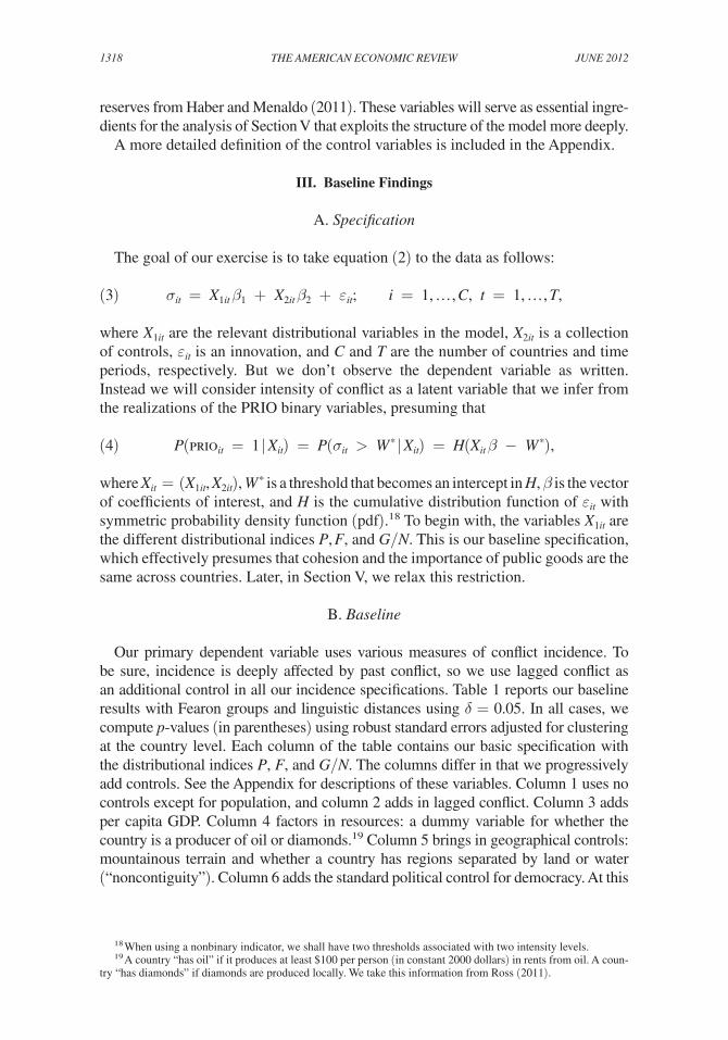
Our primary dependent variable uses various measures of conflict incidence. To be sure, incidence is deeply affected by past conflict, so we use lagged conflict as an additional control in all our incidence specifications. Table 1 reports our baseline results with Fearon groups and linguistic distances using δ = 0.05. In all cases, we compute p-values (in parentheses) using robust standard errors adjusted for clustering at the country level. Each column of the table contains our basic specification with the distributional indices p, f, and G/n. The columns differ in that we progressively add controls. See the Appendix for descriptions of these variables. Column 1 uses no controls except for population, and column 2 adds in lagged conflict. Column 3 adds per capita GDP. Column 4 factors in resources: a dummy variable for whether the country is a producer of oil or diamonds.19 Column 5 brings in geographical controls: mountainous terrain and whether a country has regions separated by land or water (“noncontiguity”). Column 6 adds the standard political control for democracy. At this
18 When using a nonbinary indicator, we shall have two thresholds associated with two intensity levels.19 A country “has oil” if it produces at least $100 per person (in constant 2000 dollars) in rents from oil. A coun-
try “has diamonds” if diamonds are produced locally. We take this information from Ross (2011).
1319EsTEBAn ET AL.: EThniciTy And confLicT: An EmpiRicAL sTudyVoL. 102 no. 4
stage, the set of controls we use is in line with MRQ, and we use this as our baseline control set. Column 7 adds in more political and governance controls.
Throughout, p, f, and G/n are significant. p has the expected positive coefficient and is highly significant. The coefficient associated with f is also positive; G/n, while also significant, has negative sign; we interpret this below. Moreover, lagged conflict is highly significant and, in line with a common result in all the literature on conflict with cross-country data, per capita income is significantly and negatively correlated with conflict.20 Finally, we do not see a direct effect of natural resources,
20 We have also examined the effect of income inequality. Using the Gini of personal incomes as a regressor has no effect either on the value of the coefficient corresponding to p or on its significance.
Table 1—Baseline Specification with prio25, Fearon Groupings
Variable (1) (2) (3) (4) (5) (6) (7)
p 7.73***(0.005)
6.07***(0.002)
6.90***(0.000)
6.96***(0.001)
7.38***(0.001)
7.39***(0.001)
6.50***(0.004)
f 2.59***(0.000)
1.86***(0.000)
1.13**(0.029)
1.09**(0.042)
1.30**(0.012)
1.30**(0.012)
1.25**(0.020)
G/n −6.95*(0.067)
−5.47**(0.011)
−4.37*(0.077)
−4.45*(0.071)
−4.77*(0.072)
−4.80*(0.068)
−5.09*(0.074)
pop 0.30***(0.009)
0.19**(0.014)
0.23**(0.012)
0.22**(0.012)
0.13(0.141)
0.13(0.141)
0.14(0.131)
gdppc — — −0.40***(0.001)
−0.41***(0.002)
−0.47***(0.001)
−0.47***(0.001)
−0.38**(0.011)
oil/diam — — — 0.06(0.777)
0.04(0.858)
0.04(0.870)
−0.10(0.643)
mount — — — — 0.01(0.134)
0.01(0.136)
0.01(0.145)
ncont — — — — 0.84**(0.019)
0.85**(0.018)
0.90**(0.011)
democ — — — — — −0.02(0.944)
0.02(0.944)
excons — — — — — — −0.13(0.741)
autocr — — — — — — 0.14(0.609)
polrights — — — — — — 0.17(0.614)
civlib — — — — — — 0.16(0.666)
lag — 2.91***(0.000)
2.81***(0.000)
2.80***(0.000)
2.73***(0.000)
2.73***(0.000)
2.79***(0.000)
const −7.28***(0.000)
−6.20***(0.000)
−3.33**(0.023)
−3.20**(0.028)
−1.47(0.326)
−1.49(0.322)
−2.42(0.147)
Pseudo-R2 0.13 0.37 0.38 0.38 0.39 0.39 0.40Observations 1,289 1,149 1,125 1,125 1,125 1,125 1,013c 141 141 138 138 138 138 137
notes: p-values are reported in parentheses. Robust standard errors adjusted for clustering have been employed to compute z-statistics.
*** Significant at the 1 percent level. ** Significant at the 5 percent level. * Significant at the 10 percent level.
1320 ThE AmERicAn Economic REViEW JunE 2012
though when this is used to construct a measure of relative publicness and interacted with distributional measures in the way suggested by the theory, it will have a highly significant impact (see Table 9).
Using the theory summarized in Proposition 1 and the assumption that α and λ are constant across countries, it is possible to provide an interpretation for the estimated parameters. First, the fact that p is highly significant suggests that both the publicness of the prize (λ) as well as the degree of group cohesion (α) are significant. Moreover, our results for G/n suggest that α is close to or perhaps even larger than 1, indicating that models of free-riding are perhaps less relevant than we make them out to be, at least in the cases of civil conflict in the data.21 One obvious possibility is selection: observed conflicts must have been successful in resolving the collective action prob-lem, so that such conflicts must be associated with a high value of group cohesion.
As for the public component, whether it is economic (control of a labor or housing market, or a trade), cultural (the establishment of some notion of ideological or reli-gious superiority), or political (control of the state) is something we cannot identify. All we can say is that it is central to conflict. At the same time, the significance of f suggests that private components, such as the existence of natural resources, are also important. While natural resources in and of themselves are not significant in our regressions, we shall see in Section V that they come fully into their own when interacted with the distributional variables as directed by the theory.
Our interpretation—that both public and private goods matter for conflict—is relevant to the discussion on greed versus grievance as motivations for ethnic conflict introduced by Collier and Hoeffler.22 While we are not sure of the utility of this distinction, one possible interpretation is that “greed” corresponds to con-flict over private goods, while “grievance” would come under the rubric of public goods (political rights and freedoms, or religious dominance). Our exercise points to the importance of both motives, and this will be enhanced further as we exploit the model structure even more in Section V.
Finally, we point to the quantitative importance of polarization and fractional-ization in conflict. Consider the baseline set of controls (Table 1, column 6). Our estimated coefficients imply that if we move from the 20th percentile of polariza-tion to the 80th percentile, holding all other variables at their means, the prob-ability of conflict rises from approximately 13 percent to 29 percent. Performing the same exercise for f takes us from 12 percent to 25 percent. These are similar (and strong) effects.
C. country Examples and scatters
Here are some country-specific examples to accompany the main findings of Table 1. This is an interesting task, as both polarization and fractionalization are positively related to conflict, but they are related to each other in a nonmonotonic way. Our strategy, then, is to work off the marginals (polarization controlling for fractionalization, and vice versa).
21 The observation that α > 1 means that individuals might effectively be placing more weight on the group than they do on themselves.
22 See Collier and Hoeffler (2004) and, more recently, Collier, Hoeffler, and Rohner (2009).
1321EsTEBAn ET AL.: EThniciTy And confLicT: An EmpiRicAL sTudyVoL. 102 no. 4
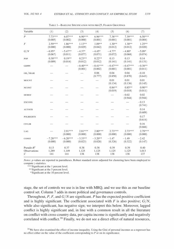
Chile exhibits the median fractionalization in our country set. If we focus on countries in the 45–55th percentiles of f and rank these countries in increasing order of polarization, we obtain the list in Table 2, panel A. Similarly, Taiwan exhibits the median polarization in the sample. Once again, if we restrict attention to countries in the 45–55th percentiles of p and rank them in increasing order of fractionaliza-tion, we obtain the list in Table 2, panel B. In each case, the first numerical column lists the intensity of conflict (at the worst point during 1960–2008): 0 when deaths fall below the prio25 threshold, 1 when that threshold is crossed but not the higher prio1000 mark, and 2 when the latter threshold is exceeded. The second numeri-cal column records the number of years of conflict incidence in the period 1960–2008: it could well exceed the total number of years in the sample (as in the case of Myanmar) if there are multiple conflicts.
Even with no other controls in this table, it is fair to say that the results are sup-portive of the econometric findings in Table 1 and in the tables to follow. Controlling for fractionalization, higher polarization goes with higher conflict, and the same is true of fractionalization once we control for polarization.
To be sure, it is too much to assert that every conflict in our dataset is ethnic in nature, and that our ethnic variables capture them fully.23 Consider China, or Haiti, or undivided Korea, which have experienced conflict and yet have low polarization and fractionalization. All conflict is not ethnic. What is remarkable is that many of them are.
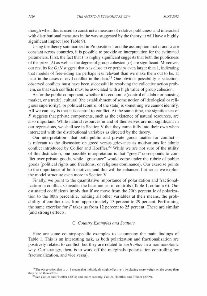
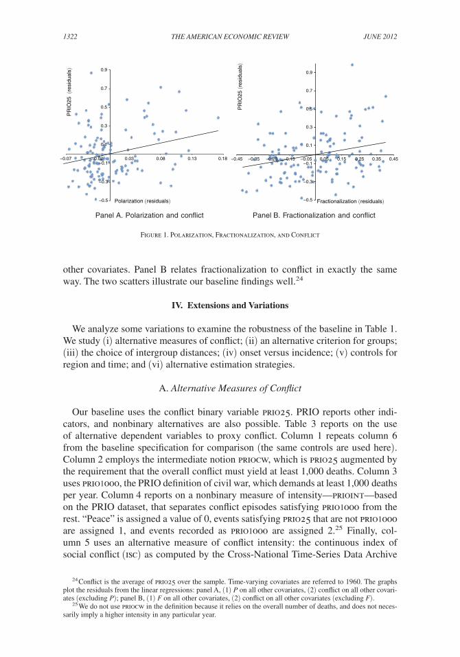
We end this section by illustrating our baseline regression with scatter plots that capture the marginal effects of polarization and fractionalization on conflict. Figure 1 does this. Panel A shows how polarization is related to conflict, conditioning by
23 To explore whether our results are driven by a particular group of observations, we have employed several tools to detect the influential observations in the sample. There are 78, 43, and 117 influential observations accord-ing to the Pearson residual, deviance residual, and Pregibon leverage statistics, respectively. The online Appendix reproduces column 6 in Table 1 once influential observations have been removed from the sample. The significance of p and f remains unaffected.
Table 2—Distribution and Conflict with Country Examples
Panel A Intensity Years Panel B Intensity Years
Dom. Rep. 1 1 Germany 0 0Morocco 1 15 Armenia 0 0US 0 0 Austria 0 0Serbia-Mont. 2 2 Taiwan 0 0Spain 1 5 Algeria 2 22Macedonia 1 1 Zimbabwe 2 9 Chile 1 1 Belgium 0 0Panama 1 1 US 0 0Nepal 2 14 Morocco 1 15Canada 0 0 Serbia-Mont. 2 2Myanmar 2 117 Latvia 0 0Kyrgystan 0 0 Trin. Tob. 1 1Sri Lanka 2 26 Guinea-Bissau 1 13Estonia 0 0 Sierra Leone 2 10Guatemala 1 30 Mozambique 2 27
notes: Panel A ranks the median fractionalization decile in increasing order of polarization. Panel B ranks the median polarization decile in increasing order of fractionalization.
1322 ThE AmERicAn Economic REViEW JunE 2012
other covariates. Panel B relates fractionalization to conflict in exactly the same way. The two scatters illustrate our baseline findings well.24
IV. Extensions and Variations
We analyze some variations to examine the robustness of the baseline in Table 1. We study (i) alternative measures of conflict; (ii) an alternative criterion for groups; (iii) the choice of intergroup distances; (iv) onset versus incidence; (v) controls for region and time; and (vi) alternative estimation strategies.
A. Alternative measures of conflict
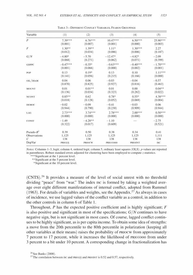
Our baseline uses the conflict binary variable prio25. PRIO reports other indi-cators, and nonbinary alternatives are also possible. Table 3 reports on the use of alternative dependent variables to proxy conflict. Column 1 repeats column 6 from the baseline specification for comparison (the same controls are used here). Column 2 employs the intermediate notion priocw, which is prio25 augmented by the requirement that the overall conflict must yield at least 1,000 deaths. Column 3 uses prio1000, the PRIO definition of civil war, which demands at least 1,000 deaths per year. Column 4 reports on a nonbinary measure of intensity—prioint—based on the PRIO dataset, that separates conflict episodes satisfying prio1000 from the rest. “Peace” is assigned a value of 0, events satisfying prio25 that are not prio1000 are assigned 1, and events recorded as prio1000 are assigned 2.25 Finally, col-umn 5 uses an alternative measure of conflict intensity: the continuous index of social conflict (isc) as computed by the Cross-National Time-Series Data Archive
24 Conflict is the average of prio25 over the sample. Time-varying covariates are referred to 1960. The graphs plot the residuals from the linear regressions: panel A, (1) p on all other covariates, (2) conflict on all other covari-ates (excluding p); panel B, (1) f on all other covariates, (2) conflict on all other covariates (excluding f).
25 We do not use priocw in the definition because it relies on the overall number of deaths, and does not neces-sarily imply a higher intensity in any particular year.
−0.5
−0.3
−0.1
0.1
0.3
0.5
0.7
0.9
0.9
−0.07 −0.02 0.03 0.08 0.13 0.18
PR
IO25
(re
sidu
als)
Polarization (residuals)
Panel A. Polarization and con�ict
−0.5
−0.3
−0.1
0.1
0.3
0.5
0.7
0.9
−0.45 −0.35 −0.25 −0.15 −0.05 0.05 0.15 0.25 0.35 0.45
PR
IO25
(res
idua
ls)
Fractionalization (residuals)
Panel B. Fractionalization and con�ict
Figure 1. Polarization, Fractionalization, and Conflict
1323EsTEBAn ET AL.: EThniciTy And confLicT: An EmpiRicAL sTudyVoL. 102 no. 4
(CNTS).26 It provides a measure of the level of social unrest with no threshold dividing “peace” from “war.” The index isc is formed by taking a weighted aver-age over eight different manifestations of internal conflict, adopted from Rummel (1963). For details of variables and weights, see the Appendix.27 As always in cases of incidence, we use lagged values of the conflict variable as a control, in addition to the other controls in column 6 of Table 1.
Throughout, p has the expected positive coefficient and is highly significant; f is also positive and significant in most of the specifications; G/n continues to have negative sign, but is not significant in most cases. Of course, lagged conflict contin-ues to be highly significant, as is per capita income. To obtain some idea of strengths: a move from the 20th percentile to the 80th percentile in polarization (keeping all other variables at their means) raises the probability of priocw from approximately 7 percent to 17 percent, while it increases the likelihood of prio1000 from under 3 percent to a bit under 10 percent. A corresponding change in fractionalization has
26 See Banks (2008).27 The correlation between isc and prio25 and prioint is 0.52 and 0.57, respectively.
Table 3—Different Conflict Variables, Fearon Groupings
Variable (1) (2) (3) (4) (5)
p 7.39***(0.001)
6.76***(0.007)
10.47***(0.001)
6.50***(0.000)
25.90***(0.003)
f 1.30**(0.012)
1.39**(0.034)
1.11*(0.086)
1.30***(0.006)
2.27(0.187)
G/n −4.80*(0.068)
−5.70(0.271)
−12.47*(0.062)
−4.82*(0.071)
−2.09(0.399)
gdppc −0.47***(0.001)
−0.35*(0.066)
−0.63***(0.000)
−0.40***(0.002)
−1.70***(0.001)
pop 0.13(0.141)
0.19*(0.056)
0.13(0.215)
0.10(0.166)
1.11***(0.000)
oil/diam 0.04(0.870)
0.06(0.825)
−0.03(0.927)
−0.04(0.816)
−0.57(0.463)
mount 0.01(0.136)
0.01**(0.034)
0.01(0.323)
0.00(0.282)
0.04**(0.022)
ncont 0.85**(0.018)
0.62(0.128)
0.78*(0.052)
0.55*(0.069)
4.38***(0.004)
democ −0.02(0.944)
−0.09(0.790)
−0.41(0.230)
−0.03(0.909)
0.06(0.944)
lag 2.73***(0.000)
3.74***(0.000)
2.78***(0.000)
2.00***(0.000)
0.50***(0.000)
const −1.49(0.322)
−4.28**(0.017)
−1.10(0.609)
— −2.75(0.521)
Pseudo-R2 0.39 0.50 0.38 0.34 0.41Observations 1,125 1,125 1,125 1,125 1,111c 138 138 138 138 138DepVar prio25 priocw prio1000 prioint isc
notes: Columns 1–3, logit; column 4, ordered logit; column 5, ordinary least squares (OLS). p-values are reported in parentheses. Robust standard errors adjusted for clustering have been employed to compute z-statistics.
*** Significant at the 1 percent level. ** Significant at the 5 percent level. * Significant at the 10 percent level.

1324 ThE AmERicAn Economic REViEW JunE 2012
similar effects: priocw goes from under 7 percent to 16 percent, while prio1000 increases from approximately 3 percent to 6 percent.
While our results are generally robust to the choice of other dependent variables, we record our own preferences. The variable prio25 is generally useful, because it serves as a repository of all conflicts. In contrast, prio1000 will fail to register conflicts that run into hundreds of deaths per year. To be sure, the choice will depend on the questions being asked, but there is no way in which our theory allows us to eliminate (as examples) the Palestinian or Guatemalan conflicts, neither of which receive a coding in any year of the PRIO dataset (up to 2008) as a prio1000 conflict. Moreover, the cumulative deaths in all these cases are sizable.28 This motivates our strong preference for PRIO’s own baseline definition of conflict using prio25, and in what follows, we will not emphasize prio1000 any longer.
Another option, and one that we have a distinct preference for, is the use of prioint, which places larger weight on prio1000 conflicts as described above. We use prio25 only because it is standard, but prioint performs just as well in every one of the regressions displayed for prio25. The online Appendix contains a full set of estimations using prioint.
B. Alternative Groupings
We have already discussed the classification of ethnic groups in Fearon (2003a). It is one that we use with some confidence, because of the deep recognition of endo-geneity in his discussion and the careful attempts made to avoid such issues. Yet, at some level, the ethnic groupings do reflect contemporary relevance. The cases of Rwanda, Burundi, or Somalia, in which there is full homogeneity in language, or of Papua, where no linguistic group reaches one percent of the population, clearly suggest that the definition of the “relevant” ethnic groups often involves careful but active intervention by the researcher.
In the interests of robustness, then, we use entirely ungrouped raw information on the size of different linguistic groups—and linguistic groups alone—provided by Ethnologue.29 The Ethnologue project lists 6,912 known living languages and gives the population sizes that use each language in each country.30 Speaking a different language certainly sets a barrier with one’s neighbor and can be considered a sound though distant base for differences in preferences for public goods. While it is ludi-crous to suggest that modern-day conflicts take place across the groups recorded in Ethnologue, it is reasonable to expect that such language distinctions could form the basis of cultural and social differences. The econometric advantage of that connec-tion is obvious: it permits a more adequate defense of exogeneity, possibly at the expense of direct causality. This is a standard trade-off.31
28 There are many other examples. To choose a current one, the Indian government has described the ongoing Maoist conflict in tribal areas as the greatest internal security threat to the country. Yet, while the conflict has been severe, with many killings, the annual numbers have been in the hundreds, but below the prio1000 threshold, as of 2010.
29 The information from Ethnologue has already been used for the analysis of conflict by Alesina et al. (2009); Desmet, Ortuño-Ortín, and Weber (2009); and Desmet, Ortuño-Ortín, and Wacziarg (2012).
30 For instance, in the case of Mexico, Ethnologue reports 291 living languages. In contrast, the number of ethnic groups for this country in Fearon’s dataset is four (Mestizo, Amerindian, White, and Mayan).
31 An alternative approach, which we have examined with equal success for p, is to instrument for the distribu-tional measures obtained from Fearon groupings using their counterparts from the Ethnologue classification. The
1325EsTEBAn ET AL.: EThniciTy And confLicT: An EmpiRicAL sTudyVoL. 102 no. 4
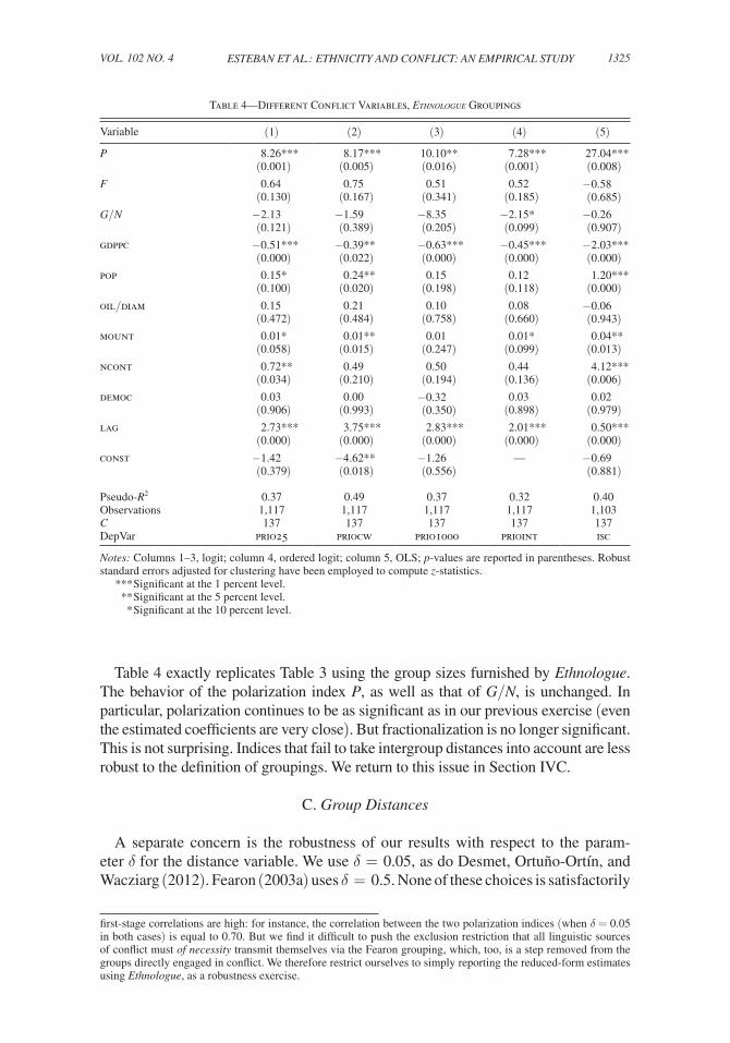
Table 4 exactly replicates Table 3 using the group sizes furnished by Ethnologue. The behavior of the polarization index p, as well as that of G/n, is unchanged. In particular, polarization continues to be as significant as in our previous exercise (even the estimated coefficients are very close). But fractionalization is no longer significant. This is not surprising. Indices that fail to take intergroup distances into account are less robust to the definition of groupings. We return to this issue in Section IVC.
C. Group distances
A separate concern is the robustness of our results with respect to the param-eter δ for the distance variable. We use δ = 0.05, as do Desmet, Ortuño-Ortín, and Wacziarg (2012). Fearon (2003a) uses δ = 0.5. None of these choices is satisfactorily
first-stage correlations are high: for instance, the correlation between the two polarization indices (when δ = 0.05 in both cases) is equal to 0.70. But we find it difficult to push the exclusion restriction that all linguistic sources of conflict must of necessity transmit themselves via the Fearon grouping, which, too, is a step removed from the groups directly engaged in conflict. We therefore restrict ourselves to simply reporting the reduced-form estimates using Ethnologue, as a robustness exercise.
Table 4—Different Conflict Variables, EthnologuE Groupings
Variable (1) (2) (3) (4) (5)
p 8.26***(0.001)
8.17***(0.005)
10.10**(0.016)
7.28***(0.001)
27.04***(0.008)
f 0.64(0.130)
0.75(0.167)
0.51(0.341)
0.52(0.185)
−0.58(0.685)
G/n −2.13(0.121)
−1.59(0.389)
−8.35(0.205)
−2.15*(0.099)
−0.26(0.907)
gdppc −0.51***(0.000)
−0.39**(0.022)
−0.63***(0.000)
−0.45***(0.000)
−2.03***(0.000)
pop 0.15*(0.100)
0.24**(0.020)
0.15(0.198)
0.12(0.118)
1.20***(0.000)
oil/diam 0.15(0.472)
0.21(0.484)
0.10(0.758)
0.08(0.660)
−0.06(0.943)
mount 0.01*(0.058)
0.01**(0.015)
0.01(0.247)
0.01*(0.099)
0.04**(0.013)
ncont 0.72**(0.034)
0.49(0.210)
0.50(0.194)
0.44(0.136)
4.12***(0.006)
democ 0.03(0.906)
0.00(0.993)
−0.32(0.350)
0.03(0.898)
0.02(0.979)
lag 2.73***(0.000)
3.75***(0.000)
2.83***(0.000)
2.01***(0.000)
0.50***(0.000)
const −1.42(0.379)
−4.62**(0.018)
−1.26(0.556)
— −0.69(0.881)
Pseudo-R2 0.37 0.49 0.37 0.32 0.40Observations 1,117 1,117 1,117 1,117 1,103c 137 137 137 137 137DepVar prio25 priocw prio1000 prioint isc
notes: Columns 1–3, logit; column 4, ordered logit; column 5, OLS; p-values are reported in parentheses. Robust standard errors adjusted for clustering have been employed to compute z-statistics.
*** Significant at the 1 percent level. ** Significant at the 5 percent level. * Significant at the 10 percent level.
1326 ThE AmERicAn Economic REViEW JunE 2012
motivated. Yet the choice is important because it implicitly selects the levels of lin-guistic (dis)similarity to be emphasized. Low values of δ will essentially separate the languages that have very few branches in common from the rest. As we pro-gressively increase δ, small differences acquire greater salience while the bigger differences play a less than proportional role. In the limit as δ → ∞, the smallest difference is identified as a complete difference, indistinguishable from deeper lin-guistic cleavages. The polarization measure that corresponds to this limit would only use binary 0–1 “distances,” and is at the heart of MRQ’s empirical study:
R = ∑ i=1
m
∑ j≠i
m
n i n j = ∑ i=1
m
n i 2 (1 − n i ).
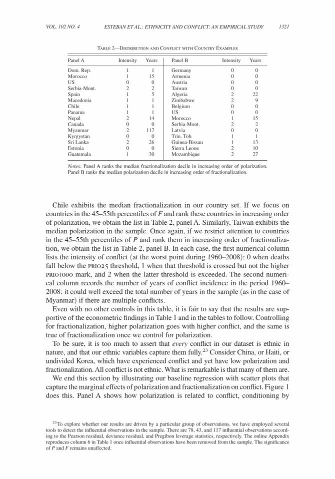
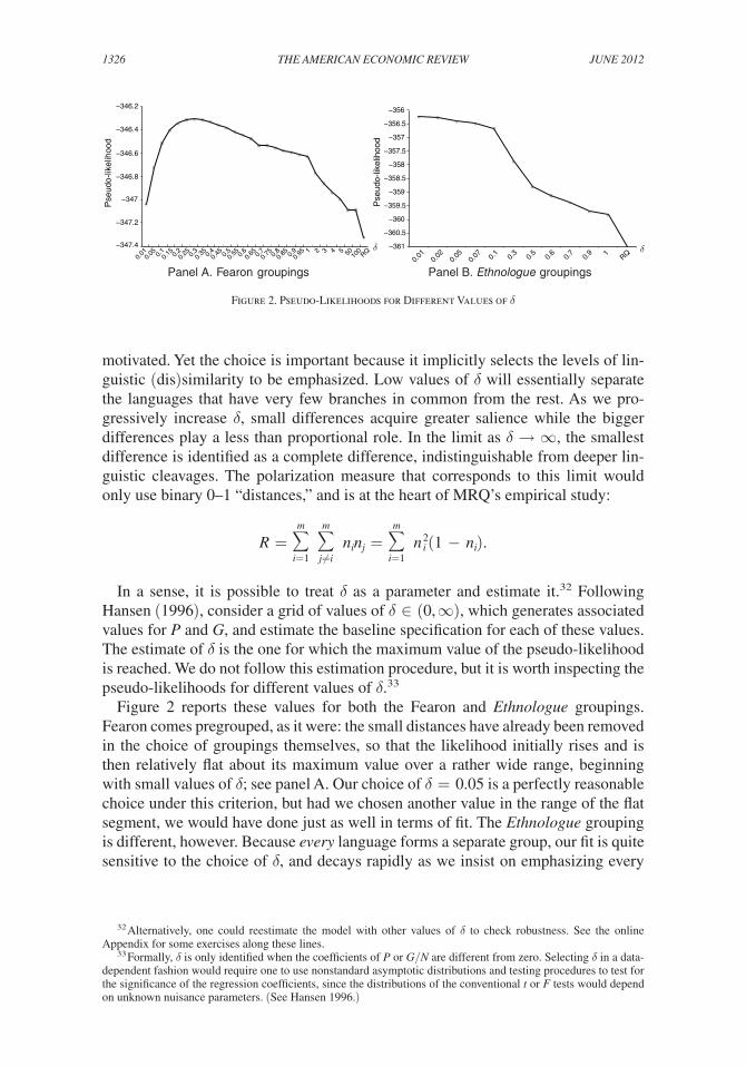
In a sense, it is possible to treat δ as a parameter and estimate it.32 Following Hansen (1996), consider a grid of values of δ ∈ (0, ∞), which generates associated values for p and G, and estimate the baseline specification for each of these values. The estimate of δ is the one for which the maximum value of the pseudo-likelihood is reached. We do not follow this estimation procedure, but it is worth inspecting the pseudo-likelihoods for different values of δ.33
Figure 2 reports these values for both the Fearon and Ethnologue groupings. Fearon comes pregrouped, as it were: the small distances have already been removed in the choice of groupings themselves, so that the likelihood initially rises and is then relatively flat about its maximum value over a rather wide range, beginning with small values of δ; see panel A. Our choice of δ = 0.05 is a perfectly reasonable choice under this criterion, but had we chosen another value in the range of the flat segment, we would have done just as well in terms of fit. The Ethnologue grouping is different, however. Because every language forms a separate group, our fit is quite sensitive to the choice of δ, and decays rapidly as we insist on emphasizing every
32 Alternatively, one could reestimate the model with other values of δ to check robustness. See the online Appendix for some exercises along these lines.
33 Formally, δ is only identified when the coefficients of p or G/n are different from zero. Selecting δ in a data-dependent fashion would require one to use nonstandard asymptotic distributions and testing procedures to test for the significance of the regression coefficients, since the distributions of the conventional t or f tests would depend on unknown nuisance parameters. (See Hansen 1996.)
Figure 2. Pseudo-Likelihoods for Different Values of δ
−347.4
−347.2
−347
−346.8
−346.6
−346.4
−346.2P
seud
o-lik
elih
ood
Panel A. Fearon groupings
−361
−360.5
−360
−359.5
−359
−358.5
−358
−357.5
−357
−356.5
−356
0.01
0.
02
0.05
0.
07
0.1
0.3
0.5
0.6
0.7
0.9 1
RQ
Pse
udo-
likel
ihoo
d
Panel B. Ethnologue groupings
δ δ0.
01 0.
05 0.
1 0.
15 0.
2 0.
25 0.
3 0.
35 0.
4 0.
45 0.
5 0.
55 0.
6 0.
65 0.
7 0.
75 0.
8 0.
85 0.
9 0.
95 1 2 3 4 5 50
10
0 RQ

1327EsTEBAn ET AL.: EThniciTy And confLicT: An EmpiRicAL sTudyVoL. 102 no. 4
language difference as important; i.e., as we raise the value of δ; see panel B and note that the axes in panels A and B have very different scales.
We illustrate this argument in the special case of the “binary” polarization mea-sure R which, as we’ve noted, effectively sets δ = ∞. The correlation between p (with δ = 0.05) and R is 0.45; see the online Appendix for the scatter plot. In Table 5, column 1 reproduces the baseline estimates for prio25 from column 6 of Table 1, using the Fearon groupings. Column 2 replaces p with the binary index R. The parallels between the two are evident: R simply takes over from p. This column can be viewed as a replication of the basic equation in MRQ. Column 3 of the table puts together both p and R along with the other distributional equations into a single equation. The comparison continues to yield symmetric outcomes: now p and R are both significant, and on very similar terms. Thus, while p is a powerful explanatory variable, so, it seems, is R.
There is a striking difference, however, once we employ classifications based on completely ungrouped linguistic criteria. Now it is imperative to carry a
Table 5—P (with δ = 0.05) versus R, Fearon and EthnologuE Groupings
Variable (1) (2) (3) (4) (5) (6)
p 7.39***(0.001)
— 5.87***(0.009)
8.26***(0.001)
— 9.02***(0.000)
f 1.30**(0.012)
0.45(0.493)
0.56(0.388)
0.64(0.130)
0.63(0.192)
0.79(0.108)
R — 7.13***(0.004)
5.12**(0.046)
— 1.09(0.560)
−1.52(0.418)
G/n −4.80*(0.068)
− 0.90(0.562)
−4.38*(0.080)
−2.13(0.121)
0.05(0.953)
−2.29*(0.100)
gdppc −0.47***(0.001)
−0.56***(0.000)
−0.57***(0.000)
−0.51***(0.000)
−0.45***(0.001)
−0.48***(0.000)
pop 0.13(0.141)
0.23***(0.005)
0.15*(0.078)
0.15*(0.100)
0.20***(0.030)
0.15(0.105)
oil/diam 0.04(0.870)
0.07(0.739)
0.08(0.712)
0.15(0.472)
0.11(0.598)
0.13(0.544)
mount 0.01(0.136)
0.01(0.162)
0.00(0.344)
0.01*(0.058)
0.01**(0.025)
0.01**(0.048)
ncont 0.85**(0.018)
0.82**(0.015)
0.93***(0.010)
0.72**(0.034)
0.51(0.116)
0.72**(0.033)
democ −0.02(0.944)
0.04(0.883)
−0.01(0.977)
0.03(0.906)
0.10(0.703)
0.01(0.977)
lag 2.73***(0.000)
2.74***(0.000)
2.70***(0.000)
2.73***(0.000)
2.80***(0.000)
2.73***(0.000)
const −1.49(0.322)
−2.75*(0.053)
−1.31(0.393)
−1.42(0.379)
−2.54(0.107)
−1.50(0.345)
Pseudo-R2 0.39 0.38 0.39 0.37 0.36 0.37Observations 1,125 1,125 1,125 1,117 1,117 1,117c 138 138 138 137 137 137Groups Fearon Fearon Fearon Eth Eth Eth
notes: Dependent variable is prio25. p-values are reported in parentheses. Robust standard errors adjusted for clus-tering have been employed to compute z-statistics.
*** Significant at the 1 percent level. ** Significant at the 5 percent level. * Significant at the 10 percent level.
1328 ThE AmERicAn Economic REViEW JunE 2012
notion of distance, otherwise every pair of groups will appear equally distinct. To see this, consider our specification using Ethnologue; we’ve reproduced col-umn 1 from Table 4 as column 4 here. Once again, p is highly significant. But this time the replacement of p by R in column 5 is not met with equal success, or indeed with any success at all; R is entirely insignificant. Finally, the horse race between p and R in column 6 is resolved unambiguously in favor of p: R plays no role at all.
The reason why R might be problematic is simple. Ethnologue groupings are fully linguistic in nature. It is reasonable to presume that conflict in society did not follow every such linguistic division. Allowing this outcome to be tempered by a consid-eration of intergroup distances (even the linguistic “distances” that we adopt in the interest of exogeneity) helps enormously. Binary measures of polarization are too coarse to achieve this modulation in any meaningful way. The data fully support such an assertion.
D. onset versus incidence
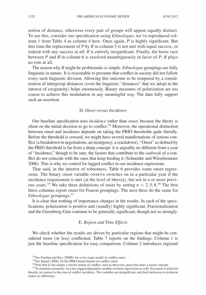
Our baseline specification uses incidence rather than onset, because the theory is silent on the initial decision to go to conflict.34 Moreover, the operational distinction between onset and incidence depends on taking the PRIO thresholds quite literally. Before the threshold is crossed, we might have several manifestations of serious con-flict (a breakdown in negotiations, an insurgency, a crackdown). “Onset” as defined by the PRIO threshold is far from a sharp concept: it is arguably no different from a year of “incidence,” though to be sure, the factors that contribute to the outbreak of a con-flict do not coincide with the ones that keep feeding it (Schneider and Wiesehomeier 2006). This is why we control for lagged conflict in our incidence regressions.
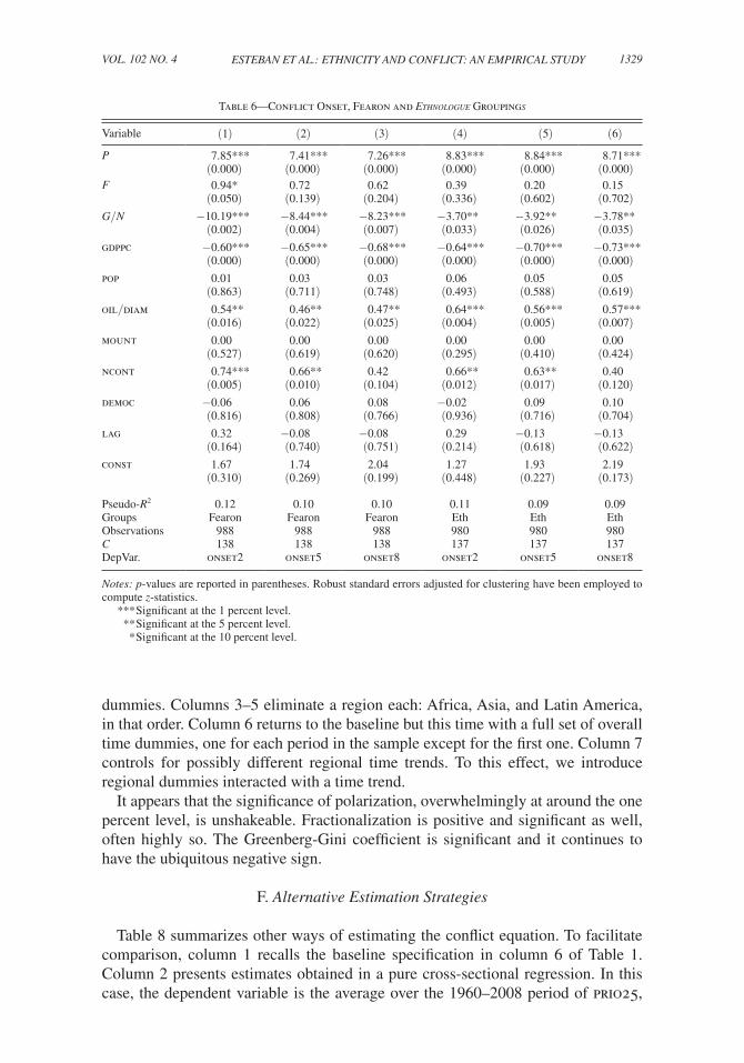
That said, in the interest of robustness, Table 6 provides some onset regres-sions. The binary onset variable onset n switches on in a particular year if the incidence requirement is met (at the level of prio25), but not in n or more previ-ous years.35 We take three definitions of onset by setting n = 2, 5, 8.36 The first three columns report onset for Fearon groupings. The next three do the same for Ethnologue groupings.37
It is clear that nothing of importance changes in the results. In each of the speci-fications, polarization is positive and (usually) highly significant. Fractionalization and the Greenberg-Gini continue to be generally significant, though not as strongly.
E. Region and Time Effects
We check whether the results are driven by particular regions that might be con-sidered more (or less) conflictual. Table 7 reports on the findings. Column 1 is just the baseline specification for easy comparison. Column 2 introduces regional
34 See Esteban and Ray (2008b) for a two-stage model of conflict onset.35 See Strand (2006) for the PRIO-based dataset on conflict onset.36 Note that if one adopts a stricter notion of conflict, such as prio1000, peace becomes a looser concept.37 To maintain symmetry, we carry lagged dependent variables in these regressions as well. Not much is achieved
thereby, in contrast to the case of conflict incidence. The variables are insignificant, and their inclusion or exclusion makes no difference.
1329EsTEBAn ET AL.: EThniciTy And confLicT: An EmpiRicAL sTudyVoL. 102 no. 4
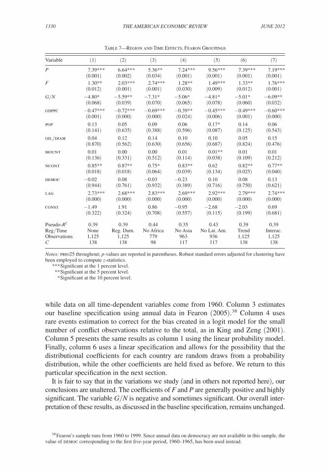
dummies. Columns 3–5 eliminate a region each: Africa, Asia, and Latin America, in that order. Column 6 returns to the baseline but this time with a full set of overall time dummies, one for each period in the sample except for the first one. Column 7 controls for possibly different regional time trends. To this effect, we introduce regional dummies interacted with a time trend.
It appears that the significance of polarization, overwhelmingly at around the one percent level, is unshakeable. Fractionalization is positive and significant as well, often highly so. The Greenberg-Gini coefficient is significant and it continues to have the ubiquitous negative sign.
F. Alternative Estimation strategies
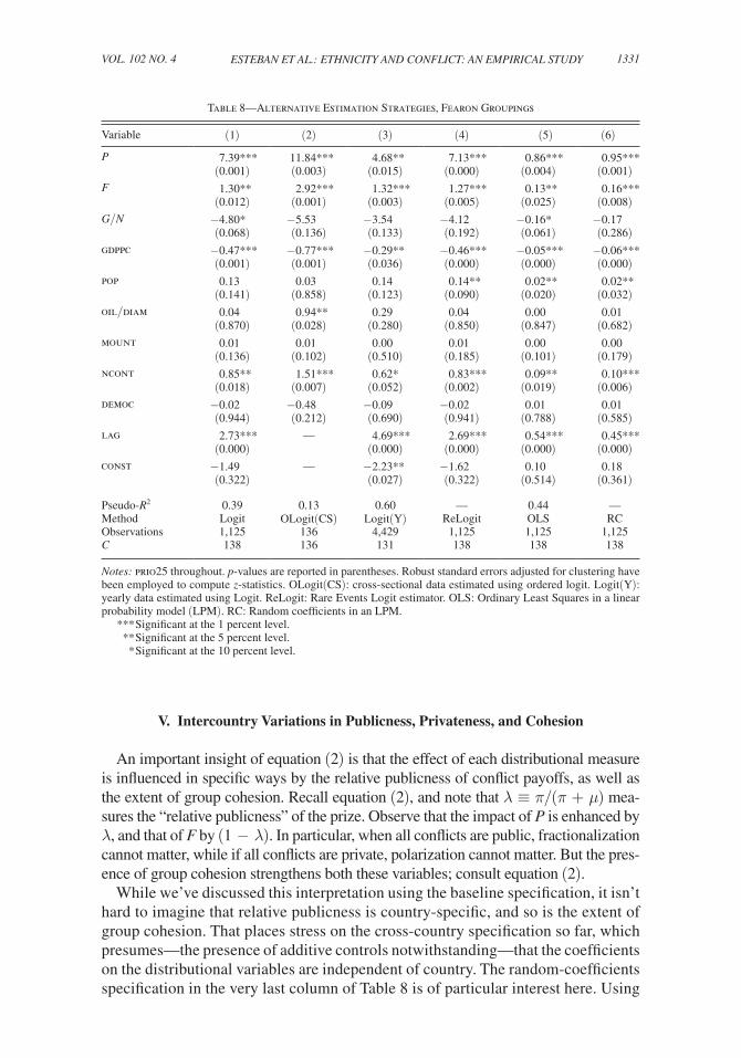
Table 8 summarizes other ways of estimating the conflict equation. To facilitate comparison, column 1 recalls the baseline specification in column 6 of Table 1. Column 2 presents estimates obtained in a pure cross-sectional regression. In this case, the dependent variable is the average over the 1960–2008 period of prio25,
Table 6—Conflict Onset, Fearon and EthnologuE Groupings
Variable (1) (2) (3) (4) (5) (6)
p 7.85***(0.000)
7.41***(0.000)
7.26***(0.000)
8.83***(0.000)
8.84***(0.000)
8.71***(0.000)
f 0.94*(0.050)
0.72(0.139)
0.62(0.204)
0.39(0.336)
0.20(0.602)
0.15(0.702)
G/n −10.19***(0.002)
−8.44***(0.004)
−8.23***(0.007)
−3.70**(0.033)
−3.92**(0.026)
−3.78**(0.035)
gdppc −0.60***(0.000)
−0.65***(0.000)
−0.68***(0.000)
−0.64***(0.000)
−0.70***(0.000)
−0.73***(0.000)
pop 0.01(0.863)
0.03(0.711)
0.03(0.748)
0.06(0.493)
0.05(0.588)
0.05(0.619)
oil/diam 0.54**(0.016)
0.46**(0.022)
0.47**(0.025)
0.64***(0.004)
0.56***(0.005)
0.57***(0.007)
mount 0.00(0.527)
0.00(0.619)
0.00(0.620)
0.00(0.295)
0.00(0.410)
0.00(0.424)
ncont 0.74***(0.005)
0.66**(0.010)
0.42(0.104)
0.66**(0.012)
0.63**(0.017)
0.40(0.120)
democ −0.06(0.816)
0.06(0.808)
0.08(0.766)
−0.02(0.936)
0.09(0.716)
0.10(0.704)
lag 0.32(0.164)
−0.08(0.740)
−0.08(0.751)
0.29(0.214)
−0.13(0.618)
−0.13(0.622)
const 1.67(0.310)
1.74(0.269)
2.04(0.199)
1.27(0.448)
1.93(0.227)
2.19(0.173)
Pseudo-R2 0.12 0.10 0.10 0.11 0.09 0.09Groups Fearon Fearon Fearon Eth Eth EthObservations 988 988 988 980 980 980c 138 138 138 137 137 137DepVar. onset2 onset5 onset8 onset2 onset5 onset8
notes: p-values are reported in parentheses. Robust standard errors adjusted for clustering have been employed to compute z-statistics.
*** Significant at the 1 percent level. ** Significant at the 5 percent level. * Significant at the 10 percent level.
1330 ThE AmERicAn Economic REViEW JunE 2012
while data on all time-dependent variables come from 1960. Column 3 estimates our baseline specification using annual data in Fearon (2005).38 Column 4 uses rare events estimation to correct for the bias created in a logit model for the small number of conflict observations relative to the total, as in King and Zeng (2001). Column 5 presents the same results as column 1 using the linear probability model. Finally, column 6 uses a linear specification and allows for the possibility that the distributional coefficients for each country are random draws from a probability distribution, while the other coefficients are held fixed as before. We return to this particular specification in the next section.
It is fair to say that in the variations we study (and in others not reported here), our conclusions are unaltered. The coefficients of f and p are generally positive and highly significant. The variable G/n is negative and sometimes significant. Our overall inter-pretation of these results, as discussed in the baseline specification, remains unchanged.
38 Fearon’s sample runs from 1960 to 1999. Since annual data on democracy are not available in this sample, the value of democ corresponding to the first five-year period, 1960–1965, has been used instead.
Table 7—Region and Time Effects, Fearon Groupings
Variable (1) (2) (3) (4) (5) (6) (7)
p 7.39***(0.001)
6.64***(0.002)
5.36**(0.034)
7.24***(0.001)
9.56***(0.001)
7.39***(0.001)
7.19***(0.001)
f 1.30**(0.012)
2.03***(0.001)
2.74***(0.001)
1.28**(0.030)
1.49***(0.009)
1.33**(0.012)
1.76***(0.001)
G/n −4.80*(0.068)
−5.59**(0.039)
−7.31*(0.070)
−5.06*(0.065)
−4.81*(0.078)
−5.01*(0.060)
−6.09**(0.032)
gdppc −0.47***(0.001)
−0.72***(0.000)
−0.69***(0.000)
−0.39**(0.024)
−0.45***(0.006)
−0.49***(0.001)
−0.60***(0.000)
pop 0.13(0.141)
0.05(0.635)
0.09(0.388)
0.06(0.596)
0.17*(0.087)
0.14(0.125)
0.06(0.543)
oil/diam 0.04(0.870)
0.12(0.562)
0.14(0.630)
0.10(0.656)
0.10(0.687)
0.05(0.824)
0.15(0.476)
mount 0.01(0.136)
0.00(0.331)
0.00(0.512)
0.01(0.114)
0.01**(0.038)
0.01(0.109)
0.01(0.212)
ncont 0.85**(0.018)
0.87**(0.018)
0.75*(0.064)
0.83**(0.039)
0.62(0.134)
0.82**(0.025)
0.77**(0.040)
democ −0.02(0.944)
0.08(0.761)
−0.03(0.932)
−0.23(0.389)
0.10(0.716)
0.08(0.750)
0.13(0.621)
lag 2.73***(0.000)
2.68***(0.000)
2.83***(0.000)
2.69***(0.000)
2.92***(0.000)
2.79***(0.000)
2.74***(0.000)
const −1.49(0.322)
1.91(0.324)
0.86(0.708)
−0.95(0.557)
−2.68(0.115)
−2.03(0.199)
0.69(0.681)
Pseudo-R2 0.39 0.39 0.44 0.35 0.43 0.39 0.39Reg/Time None Reg. Dum. No Africa No Asia No Lat. Am. Trend Interac.Observations 1,125 1,125 779 963 936 1,125 1,125c 138 138 98 117 117 138 138
notes: prio25 throughout; p-values are reported in parentheses. Robust standard errors adjusted for clustering have been employed to compute z-statistics.
*** Significant at the 1 percent level. ** Significant at the 5 percent level. * Significant at the 10 percent level.
1331EsTEBAn ET AL.: EThniciTy And confLicT: An EmpiRicAL sTudyVoL. 102 no. 4
V. Intercountry Variations in Publicness, Privateness, and Cohesion
An important insight of equation (2) is that the effect of each distributional measure is influenced in specific ways by the relative publicness of conflict payoffs, as well as the extent of group cohesion. Recall equation (2), and note that λ ≡ π/(π + �) mea-sures the “relative publicness” of the prize. Observe that the impact of p is enhanced by λ, and that of f by (1 − λ). In particular, when all conflicts are public, fractionalization cannot matter, while if all conflicts are private, polarization cannot matter. But the pres-ence of group cohesion strengthens both these variables; consult equation (2).
While we’ve discussed this interpretation using the baseline specification, it isn’t hard to imagine that relative publicness is country-specific, and so is the extent of group cohesion. That places stress on the cross-country specification so far, which presumes—the presence of additive controls notwithstanding—that the coefficients on the distributional variables are independent of country. The random-coefficients specification in the very last column of Table 8 is of particular interest here. Using
Table 8—Alternative Estimation Strategies, Fearon Groupings
Variable (1) (2) (3) (4) (5) (6)
p 7.39***(0.001)
11.84***(0.003)
4.68**(0.015)
7.13***(0.000)
0.86***(0.004)
0.95***(0.001)
f 1.30**(0.012)
2.92***(0.001)
1.32***(0.003)
1.27***(0.005)
0.13**(0.025)
0.16***(0.008)
G/n −4.80*(0.068)
−5.53(0.136)
−3.54(0.133)
−4.12(0.192)
−0.16*(0.061)
−0.17(0.286)
gdppc −0.47***(0.001)
−0.77***(0.001)
−0.29**(0.036)
−0.46***(0.000)
−0.05***(0.000)
−0.06***(0.000)
pop 0.13(0.141)
0.03(0.858)
0.14(0.123)
0.14**(0.090)
0.02**(0.020)
0.02**(0.032)
oil/diam 0.04(0.870)
0.94**(0.028)
0.29(0.280)
0.04(0.850)
0.00(0.847)
0.01(0.682)
mount 0.01(0.136)
0.01(0.102)
0.00(0.510)
0.01(0.185)
0.00(0.101)
0.00(0.179)
ncont 0.85**(0.018)
1.51***(0.007)
0.62*(0.052)
0.83***(0.002)
0.09**(0.019)
0.10***(0.006)
democ −0.02(0.944)
−0.48(0.212)
−0.09(0.690)
−0.02(0.941)
0.01(0.788)
0.01(0.585)
lag 2.73***(0.000)
— 4.69***(0.000)
2.69***(0.000)
0.54***(0.000)
0.45***(0.000)
const −1.49(0.322)
— −2.23**(0.027)
−1.62(0.322)
0.10(0.514)
0.18(0.361)
Pseudo-R2 0.39 0.13 0.60 — 0.44 —Method Logit OLogit(CS) Logit(Y) ReLogit OLS RCObservations 1,125 136 4,429 1,125 1,125 1,125c 138 136 131 138 138 138
notes: prio25 throughout. p-values are reported in parentheses. Robust standard errors adjusted for clustering have been employed to compute z-statistics. OLogit(CS): cross-sectional data estimated using ordered logit. Logit(Y): yearly data estimated using Logit. ReLogit: Rare Events Logit estimator. OLS: Ordinary Least Squares in a linear probability model (LPM). RC: Random coefficients in an LPM.
*** Significant at the 1 percent level. ** Significant at the 5 percent level. * Significant at the 10 percent level.
1332 ThE AmERicAn Economic REViEW JunE 2012
a likelihood ratio test, we can indeed reject the hypothesis of constant coefficients. Statistically, this is no surprise, as such a specification across countries is often rejected anyway, though we return to this test below.39 Despite this, it is of interest that the estimates of the coefficients in the OLS-LPM and RC specifications (see columns 5 and 6 of Table 8) are very similar—these coefficients are compa-rable since they’ve both been estimated in a linear specification. That suggests that the qualitative and quantitative conclusions of the first part of the paper hold when the assumption of constancy of the coefficients is dropped.
The goal of this section, then, is to construct and use country-by-country proxies for relative publicness and cohesion.
We first construct indicators for π and �, and use these to define a proxy for the relative publicness of the prize. Begin with the indicator for the private payoff �. It seems natural to associate � with rents that are easily appropriable. Because appropriability is closely connected to the presence of resources, we approximate the degree of “privateness” in the prize by asking if the country is rich in natural resources. We proxy the abundance of natural resources by the per capita value of oil reserves (oilresv).40 Next, we create an index of “publicness” (pub) by ask-ing different questions about the degree of power afforded to those who run the country, “more democratic” being regarded as correlated with “less power” and consequently a lower valuation of the public payoff to conflict. We use four differ-ent proxies to construct the index:41 (i) the lack of executive constraints (excons); (ii) the level of autocracy (autocr); (iii) the degree to which political rights are flouted (polrights); and (iv) the extent of suppression of civil liberties (civlib). Our variable pub is constructed by looking at binary versions of these outcomes and then averaging the indicators. Details are in the Appendix. The results are robust to different modes of construction and indeed to the choice of a subset of these mea-sures; see the online Appendix for some variants.
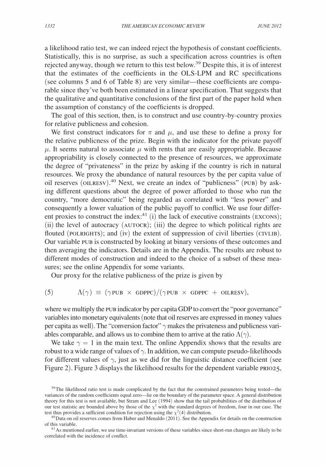
Our proxy for the relative publicness of the prize is given by
(5) Λ(γ ) ≡ (γ pub × gdppc)/(γ pub × gdppc + oilresv),
where we multiply the pub indicator by per capita GDP to convert the “poor governance” variables into monetary equivalents (note that oil reserves are expressed in money values per capita as well). The “conversion factor” γ makes the privateness and publicness vari-ables comparable, and allows us to combine them to arrive at the ratio Λ(γ).
We take γ = 1 in the main text. The online Appendix shows that the results are robust to a wide range of values of γ. In addition, we can compute pseudo-likelihoods for different values of γ, just as we did for the linguistic distance coefficient (see Figure 2). Figure 3 displays the likelihood results for the dependent variable prio25,
39 The likelihood ratio test is made complicated by the fact that the constrained parameters being tested—the variances of the random coefficients equal zero—lie on the boundary of the parameter space. A general distribution theory for this test is not available, but Stram and Lee (1994) show that the tail probabilities of the distribution of our test statistic are bounded above by those of the χ2 with the standard degrees of freedom, four in our case. The test thus provides a sufficient condition for rejection using the χ2 (4) distribution.
40 Data on oil reserves comes from Haber and Menaldo (2011). See the Appendix for details on the construction of this variable.
41 As mentioned earlier, we use time-invariant versions of these variables since short-run changes are likely to be correlated with the incidence of conflict.

1333EsTEBAn ET AL.: EThniciTy And confLicT: An EmpiRicAL sTudyVoL. 102 no. 4
and for the two empirical specifications in Table 9 that use prio25. Clearly, γ = 1 is a good choice under this criterion.
Table 9, columns 1–3, provides a variety of different specifications using the binary variable prio25 as well as the multivalued indicators prioint and isc. Group cohe-sion is held constant, and our main independent variables are p × Λ, f × (1 − Λ), and G/n × Λ, where Λ ≡ Λ(1). This allows us to test whether the interacted indi-ces of ethnic inequality, fractionalization, and polarization are significant. We also include the noninteracted indices in order to examine whether their significance truly comes from the interaction term.42 Polarization interacted with Λ is positive and generally significant, and the same is true of fractionalization interacted with 1 − Λ. (The interacted Greenberg-Gini is not significant.)
The level terms p, f, and G are now no longer significant. Conditional on hav-ing the true values of λ, this is precisely what the model would predict. After all, the influence of polarization (say) should be zero when there are no public goods, broadly defined to include primordial goals, at stake. The fact that our estimate Λ happens to achieve the same goal is of interest, and possibly suggests that factors such as pure primordialism have little to do with ethnic conflict.
We remark on the interpretation of interactions in nonlinear regressions (such as the logit). It is well known that any significance of an interaction term cannot be attributed fully to the true effect of that interaction term on the dependent variable (see, e.g., Ai and Norton 2003).43 It does imply, however, that the effect on the underlying latent variable—the cost of conflict, as proxied by the number of deaths—is indeed as esti-mated. And this is what we are interested in from the viewpoint of the theory.
Next, we allow group cohesion to vary across countries. We estimate a proxy A for the level of group cohesion α by exploiting the answers to a certain set of questions asked in the 2005 wave of the World Values survey. We use the latest wave available because it covers the largest number of countries. One could argue that the answers might be conditioned by the existence of previous or contemporary conflict. The
42 We do not include the level of Λ—there is nothing to suggest that it will have a level effect—but rather the components of Λ, which are the oilresv indicator and the variable pub × gdppc constructed from the governance variables.
43 A linear probability model, though problematic on other grounds, would not exhibit this problem.
Figure 3. Pseudo-Likelihoods for Different Values of γ
0.15
0.
25 0.
5 0.
75 1
1.25
1.
5 1.
75 2
2.5 3
3.5 4
4.5 5
5.5 6 7 8 9 10
15
20
30
Pse
uodo
-like
lihoo
d
Panel A. Without group cohesion0.
15 0.
25 0.
5 0.
75 1
1.25
1.
5 1.
75 2
2.5 3
3.5 4
4.5 5
5.5 6 7 8 9 10
15
20
30
Pse
udo-
likel
ihoo
d
Panel B. With group cohesion
γ γ

1334 ThE AmERicAn Economic REViEW JunE 2012
questions we have selected, described in detail in the Appendix, do not ask about specific groups, but address issues like adherence to social norms, identification with the local community, the importance of helping others, and so on.44 We con-struct a summary proxy for α—call it A—from the scores on these questions.
44 To be sure, even such a procedure is vulnerable to charges of endogeneity, but hopefully less so.
Table 9—Relative Publicness and Cohesion, Fearon Groupings
Variable (1) (2) (3) (4) (5) (6)
p −3.31(0.424)
−1.93(0.538)
−9.21(0.561)
−3.01(0.478)
−1.65(0.630)
−13.04(0.584)
f 0.73(0.209)
0.75(0.157)
−2.27(0.249)
1.48(0.131)
1.51(0.108)
−6.65**(0.047)
G/n −5.07(0.346)
−4.61(0.352)
0.78(0.789)
−3.78(0.767)
3.31(0.742)
−71.03(0.214)
pΛ 17.38***(0.001)
13.53***(0.001)
60.23***(0.005)
— — —
f(1 − Λ) 2.53***(0.003)
1.92***(0.003)
11.87***(0.000)
— — —
(G/n)Λ −0.72*(0.912)
−1.37(0.823)
−9.57(0.298)
— — —
pΛA — — — 23.25**(0.021)
19.16**(0.019)
72.22*(0.083)
f(1 − Λ)A — — — 4.02**(0.013)
2.92***(0.003)
26.03***(0.000)
(G/n)Λ(1 − A) — — — −2.31(0.981)
−68.42(0.358)
579.24*(0.089)
gdppc −0.62***(0.000)
−0.50***(0.000)
−2.36***(0.000)
−0.65***(0.000)
−0.53***(0.003)
−3.68***(0.000)
pop 0.10(0.267)
0.09(0.243)
0.99***(0.000)
0.08(0.622)
0.09(0.448)
0.33(0.565)
oilresv 0.00(0.986)
0.00(0.860)
0.00(0.277)
0.00**(0.017)
0.00***(0.006)
0.00(0.234)
mount 0.01*(0.059)
0.00(0.169)
0.04**(0.012)
0.02***(0.009)
0.01**(0.015)
0.06**(0.032)
ncont 0.87**(0.015)
0.41(0.173)
4.21***(0.005)
1.31***(0.002)
0.93***(0.007)
4.98***(0.008)
pubgdppc 0.00(0.397)
0.00(0.847)
0.00**(0.014)
0.00**(0.024)
0.00*(0.074)
0.00(0.214)
lag 2.62***(0.000)
1.93***(0.000)
0.47***(0.000)
2.40***(0.000)
1.79***(0.000)
0.42***(0.000)
const −0.01(0.995)
— −5.27(0.354)
−0.43(0.900)
— 28.33*(0.072)
Pseudo-R2 0.40 0.34 0.42 0.48 0.39 0.41Observations 1,104 1,104 1,090 447 447 443c 138 138 138 53 53 53DepVar. prio25 prio-int isc prio25 prio-int isc
notes: Columns 1 and 4, logit; columns 2 and 5, ordered logit; columns 3 and 6, OLS; p-values are reported in parentheses. Robust standard errors adjusted for clustering have been employed to compute z-statistics.
*** Significant at the 1 percent level. ** Significant at the 5 percent level. * Significant at the 10 percent level.
1335EsTEBAn ET AL.: EThniciTy And confLicT: An EmpiRicAL sTudyVoL. 102 no. 4
Unfortunately, a significant shortcoming of this approach is that the sample of countries even in the 2005 World Values survey is limited. We are therefore restricted to only 447 observations, corresponding to 53 countries.
Columns 4–6 of Table 9 examine this variant. In this specification the independent variables are exactly the ones posited by the model. We use precisely the combina-tions asked for by the theory: polarization is weighted both by Λ and by A, fraction-alization by (1 − Λ) and by A again, and so on. We continue to employ the direct terms p, f, and G, as well as the controls.45 The results continue to be quite striking. The composite terms for polarization and fractionalization are significant. The lev-els continue to be insignificant.
Finally, we test the hypothesis that now, with the interacted effects in place, the estimated coefficients can be taken to be common across countries. We reestimate the regressions in Table 9 by allowing for random coefficients in the interacted and noninteracted indices. This time, invoking the Stram-Lee test once again, we are unable to reject the hypothesis of constant coefficients for columns 3 to 6.46 This is by no means conclusive, but it suggests that a fair amount of intercountry variation is indeed being picked up by the new specifications of Table 9.
We remind the reader that we have reported our results using the conversion factor γ = 1 to aggregate public and private prizes in equation (5). The online Appendix reports on several versions of Table 9, for different values of γ, and shows that our results are robust to these variations.
VI. Summary and Conclusions
In a monumental treatise, Horowitz (1985, p. 92) observes of the second half of the twentieth century that “[i]n much of Asia and Africa, it is only modest hyperbole to assert that the Marxian prophecy has had an ethnic fulfillment.”
This is a remarkable assertion. The fundamental question of interest is whether ethnic “divisions” do matter for social conflict. We’ve argued that such a question cannot be addressed properly unless we have theory to guide us on the empirical construction of an “ethnic division.” As Esteban and Ray (2011) show, the appropri-ate choice of division depends on the nature of the conflict—whether it is over pub-lic or private goods—and the extent of cohesion within the groups that are engaged in conflict. In particular, that paper links ethnic conflict to a linear combination of ethnic polarization, ethnic fractionalization, and the Greenberg-Gini index of inter-group differences. As we have discussed in some detail in the paper, the weights in that linear combination correspond to the relative importance of public and pri-vate goods in the conflict prize. Specifically, the impact of polarization increases with conflict over public goods, while the impact of fractionalization increases with the private component of conflict. The Esteban-Ray framework also tells us that the importance of the three indices depends on the extent of within-group cohe-sion present in intergroup conflict. (In particular, when there is no cohesion at all, the well-known free-rider problem dominates and all conflict vanishes when the
45 We feel no particular compunction to include all possible level effects. Terms such as p × Λ × A can be viewed as composite variables that the model predicts will matter, and not as interactions of (in this instance) three variables.
46 See Table 15 in the online Appendix and the discussion there.

1336 ThE AmERicAn Economic REViEW JunE 2012
population is large.) The theoretical structure therefore both disciplines our empiri-cal specification and allows for interpretation of the estimated coefficients.
The first task of this paper is to implement the above measures; specifically, those that employ intergroup “distances.” We do so using linguistic differences across groups, in the spirit of Fearon (2003a) and Desmet, Ortuño-Ortín, and Wacziarg (2012). Linguistic distance—as constructed by the cardinality of intervening nodes on the language tree—is plausibly exogenous to conflict, while at the same time they can be expected to drive—or at least influence—antagonisms across groups.47
We then proceed to an empirical analysis that closely parallels the theory. Our main result is that ethnic polarization has a large and highly significant impact on conflict across a number of different specifications. By and large, though with somewhat lesser consistency, this is also true of fractionalization. These two findings suggest that public and private components of conflict are generally both present, and that within-group cohesion is strong during conflict.48 The numerical effects of the two measures are large and quite similar. For instance, moving polarization from the 20th percentile to the 80th percentile, holding all other variables at their means, approximately doubles the chances of conflict, and the same is true of fractionalization.
Our results concerning polarization (and to a lesser degree, fractionalization) are highly robust. They extend to a variety of different measures of conflicts (including different binary measures of conflict incidence, as well as continuous indices), to alter-native ways of calculating language distances, to different choices of groups (as long as language is principally used in defining them), to the use of different regional dum-mies or selections, and to the inclusion of overall or regional time trends.
A limitation of our cross-sectional approach is that the importance of public and private components of conflict, as well as the extent of group cohesion, are presumed not to vary over countries. We therefore pursue refinements of our specification by constructing country-specific measures of “relative publicness” of the prize, using data on natural resources (as a proxy for private payoffs) and data on autocracy (as a proxy for public payoff to holding power). We combine these measures to create an index of “relative publicness” of conflict payoffs, one that varies across countries. When our measures are interacted with this index in exactly the way suggested by the theory, the resulting coefficients are significant across a variety of specifications, and are strongly supportive of the conceptual framework.
The exercise can be augmented still further by using a measure for within-group cohesion, one that we construct by using information from the World Values survey. We can then directly address the model by imposing even more structure, by con-structing variables that conform precisely to those predicted by the theory. The result-ing outcomes, both for polarization and fractionalization, are highly significant.
This paper takes a step toward the establishment of a strong empirical relation-ship between conflict and certain indicators of ethnic group distribution, one that is
47 Another possibility, infeasible at present, is to use measures of genetic distance across groups. This is not hard to do across countries, but at this time there is too little within-country variation. In those cases in which more disag-gregated data is available (see Cavalli-Sforza, Menozzi, and Piazza 1994), it has been prohibitively difficult to obtain group share data. Perhaps in the near future, with more detailed genetic datasets, this approach will become feasible.
48 The Greenberg-Gini index (normalized by population, as required by the theory) is also significant in several of the specifications, but usually with a negative sign. This finding supports our conclusion that group cohesion is extremely important and present to a significant degree in times of conflict. Presumably, the very fact that a conflict is observed implies that free-rider problems have been overcome to a large extent.
1337EsTEBAn ET AL.: EThniciTy And confLicT: An EmpiRicAL sTudyVoL. 102 no. 4
firmly grounded in theory. Observe that in no case do we use income-based groups or income-based measures, and in this sense our study is perfectly orthogonal to those that attempt to find a relationship between economic inequality and conflict. At the same time, as we have argued in this paper, this is not to say that conflict is fundamentally noneconomic. It could be. But there is an equal possibility that the economics of conflict finds expression across groups that are demarcated on other grounds: religion, caste, geography, or language. Such markers can profitably be exploited for economic and political ends, even when the markers themselves have nothing to do with economics. A more nuanced study of the relative importance of economic versus primordial antagonisms must await future research, however.
Appendix
We provide definitions of all major variables used in the paper, beginning with the different measures of conflict.
prio25. “Armed conflict” from PRIO: a contested incompatibility that concerns government and/or territory where the use of armed force between two parties, of which at least one is the government of a state, results in at least 25 battle-related deaths per year and per incompatibility. We consider only types 3 and 4 from the database; these refer to internal armed conflict. If a country has experienced a prio25 conflict according to the PRIO dataset in any of the years of our five-year period, this variable takes a value equal to 1.
priocw. “Intermediate armed conflict” from PRIO: includes all prio25 conflicts that result in a minimum of 1,000 deaths over the course of the conflict. We consider only types 3 and 4 (internal armed conflict). If a country has experienced a priocw conflict according to the PRIO dataset in any of the years of our five-year period, this variable takes a value equal to 1.
prio1000. “War” from PRIO: same definition as prio25 with a threshold of battle-related deaths of at least 1,000 per year and per incompatibility. We consider only types 3 and 4 (internal armed conflict). If a country has experienced a prio1000 conflict according to the PRIO dataset in any of the years of our five-year period, this variable takes a value equal to 1.
prioint. “Conflict intensity” from PRIO: we assign a value of 0 if there is peace in a given year, a value of 1 if there are events satisfying prio25 that are not prio1000, and a value of 2 if there are events recorded as prio1000. The value of prioint is the maximum conflict level experienced within the five-year period.
isc. Index of social conflict. The Cross-National Time-Series Data Archive (CNTS) computes the isc index as the weighted average of eight variables related to social unrest.49
49 These variables are (weights are provided in brackets): Assassinations (domestic1) [25]: Any politically moti-vated murder or attempted murder of a high government official or politician. General Strikes (domestic2) [20]: Any strike of 1,000 or more industrial or service workers that involves more than one employer and that is aimed at national government policies or authority. Guerrilla Warfare (domestic3) [100]: Any armed activity, sabotage, or bombings carried on by independent bands of citizens or irregular forces and aimed at the overthrow of the pres-ent regime. Major Government Crises (domestic4) [20]: Any rapidly developing situation that threatens to bring the downfall of the present regime, excluding situations of revolt aimed at such overthrow. Purges (domestic5) [20]: Any systematic elimination by jailing or execution of political opposition within the ranks of the regime or the opposition. Riots (domestic6) [25]: Any violent demonstration or clash of more than 100 citizens involving

1338 ThE AmERicAn Economic REViEW JunE 2012
Next, we define the three main distributional measures that we use.f. Fractionalization, defined as f = ∑ i=1
m n i (1 − n i ), where n i is the population
share of group i and m is the number of groups. Data on group shares has been obtained from Fearon (2003b) and the Ethnologue project (http://www.ethnolgue.com).
p. Polarization, computed as p = ∑ i=1 m ∑ j=1
m n i 2 n j κ ij , where κ ij = 1 − s ij 0.05 and
s ij is the degree of similarity between two languages i and j, given by the ratio of the number of common branches to the maximum possible number—15 for the entire tree.50 Group shares are constructed as above, for f; data on language and linguistic distances come from Ethnologue.
G. Greenberg-Gini index, defined as G = ∑ i=1 m ∑ j=1
m n i n j κ ij . We use the same
data sources as for p.R. Binary-distance polarization measure, defined as R = ∑ i=1
m n i 2 (1 − n i ). We
use the same data sources as for f.Finally, we record the other variables and controls in alphabetical order.A. A variable for group cohesion, constructed from the 2005 wave of the World
Values survey. For each individual, we compute the simple average of the scores to a set of questions related to group commitment and adhesion to social norms.51 The country estimate is the average of the individual averages.
autocr. Institutionalized autocracy. The data source is Polity IV (2011) and takes values on a 0–10 scale, with 10 signifying extreme autocracy. We transform this variable into a time-invariant dummy in the following way: first, the percentage of years in the sample for which a country received a score lower than five was calcu-lated. Then, if this percentage was lower than 40 percent, a country received a time-invariant 1 for this nonautocracy dummy and 0 otherwise.
civlib. (Lack of) civil liberties. Data source is Freedom House (2011), which con-siders a 1–7 scale (1 indicates highest level of liberties). We transform this variable into a time-invariant dummy in the following way: first, the percentage of years in the sample for which a country received a score smaller than four was calculated. Then, if this percentage was smaller than 40 percent, a country received a value of 1 in all the sample.
democ. Institutionalized democracy. Data source is Polity IV (2011). Democracy ranges from 0 (low) to 10 (high). As in MRQ, democ takes a value equal to 1 if the score is higher than or equal to 4 and 0 otherwise.
excons. (Lack of) executive constraints. It is defined on a 1–7 scale (1 indicates minimum constraints); source is Polity IV (2011). We transform this variable into
the use of physical force. Revolutions (domestic7) [150]: Any illegal or forced change in the top government elite, any attempt at such a change, or any successful or unsuccessful armed rebellion whose aim is independence from the central government. Antigovernment Demonstrations (domestic8) [10]: Any peaceful public gathering of at least 100 people for the primary purpose of displaying or voicing their opposition to government policies or authority, excluding demonstrations of a distinctly antiforeign nature. The calculation of the isc is performed as follows: weighted sum of occurrences of each event divided by the number of types of variables, 8.
50 If two groups speak the same language, s ij is set to 1.51 These questions are: V84: “It is important to this person to help the people nearby; to care for their well-
being.” V87: “It is important to this person to always behave properly; to avoid doing anything people would say is wrong.” V89: “Tradition is important to this person; to follow the customs handed down by one’s religion or fam-ily.” V7: “For each of the following, indicate how important it is in your life. Would you say it is: Politics.” V9: “For each of the following, indicate how important it is in your life: Religion.” V211: “People have different views about themselves and how they relate to the world. Using this card, would you tell me how strongly you agree or disagree with each of the following statements about how you see yourself?: I see myself as part of my local community.” All variables are normalized to a 1–4 scale.

1339EsTEBAn ET AL.: EThniciTy And confLicT: An EmpiRicAL sTudyVoL. 102 no. 4
a time-invariant dummy in the following way: first, the percentage of years in the sample for which a country received a score greater than four is computed. Then, if this percentage is smaller than 0.4, a country received a value of excons equal to 1 in all the sample.
gdppc. Log of real GDP per capita corresponding to the first year of each five-year period. Source: Maddison (2008).
mount. Percent mountainous terrain. The data source is Fearon and Laitin (2003b), who use the codings of geographer A. J. Gerard.
n. Population, in millions. Source: Maddison (2011).ncont. Noncontiguous states, referring to countries with territory holding at least
10,000 people and separated from the land area containing the capital city either by land or by 100 kilometers of water. Source: Fearon and Laitin (2003b).
oil/diam. Oil/Diamond dummy, which takes the value 1 if the country is “rich in oil” or produces (any positive quantity of) diamonds. A country is “rich in oil” if the average value of its oil production in a period is larger than 100 US dollars in 2000 constant dollars. Source: Ross (2011).
oilresv. Per capita value of oil reserves at the beginning of the period. Data for oil reserves comes from Haber and Menaldo (2011). To convert quantities into dol-lars, we use the oil price data in Ross (2006), where prices are referred to the same year as reserves. Finally, we divide by population to obtain a per capita measure.
Table 10—Summary Statistics
Conflict variables Mean SD
prio25 0.231 0.422priocw 0.156 0.363prio1000 0.090 0.286prioint 0.321 0.631isc 9.317 14.436
Ethnolinguistic indices Mean SD p δ=0.05 (Fearon) 0.046 0.054G/ n δ=0.05 Fearon 0.044 0.129f (Fearon) 0.417 0.245R (Fearon) 0.123 0.063 p δ=0.05 (ETH) 0.043 0.048G/ n δ=0.05 (ETH) 0.110 0.365f (ETH) 0.451 0.319R (ETH) 0.107 0.066
Other variables Mean SDgdppc 7.985 1.111pop 15.721 1.807mount 15.518 19.853ncont 0.146 0.353dem 0.472 0.499oil/Diam 0.316 0.465oilresv 23,960.400 170,898.700pub 0.446 0.445excons 0.536 0.498autocr 0.371 0.483polrights 0.459 0.499civlib 0.475 0.500Λ 0.565 0.408A 0.729 0.073
1340 ThE AmERicAn Economic REViEW JunE 2012
polrights. (Lack of) political rights. The data source is Freedom House (2011), which considers a 1–7 scale (1 indicates most free). We transform this variable into a time-invariant dummy in the following way: first, the percentage of years in the sample for which a country received a score smaller than four was calculated. Then, if this percentage was smaller than 40 percent, a country received a value of 1 in all the sample.
pop. Log of population in the first year of each five-year period. Source: Maddison (2008).
pub. Publicness index. It is defined as the simple average of excons, autocr, polrights, and civlib.
Λ. Relative publicness of the prize, defined as Λ = pub/(pub + oilresv/gdp). It corresponds to Λ(γ) in the text when the conversion factor γ is set equal to 1.
Table 10 presents the mean and the standard deviation of all the variables employed in the empirical analysis.
REFERENCES
Ai, Chunrong, and Edward C. Norton. 2003. “Interaction Terms in Logit and Probit Models.” Econom-ics Letters 80 (1): 123–29.
Alesina, Alberto, Arnaud Devleeschauwer, William Easterly, Sergio Kurlat, and Romain Wacziarg. 2003. “Fractionalization.” Journal of Economic Growth 8 (2): 155–94.
Atlas Narodov Mira. 1964. Miklukho-Maklai Ethnological Institute at the Department of Geodesy and Cartography of the State Geological Committee of the Soviet Union: Moscow.
Banks, Arthur S. 2008. “Cross-National Time-Series Data Archive (CNTS) 1815–2007.” Databanks International, Jerusalem, Israel (accessed October 1, 2010).
Besley, Timothy, and Torsten Persson. 2010. “State Capacity, Conflict, and Development.” Economet-rica 78 (1): 1–34.
Blattman, Christopher, and Edward Miguel. 2010. “Civil War.” Journal of Economic Literature 48 (1): 3–57.
Brockett, Charles D. 1992. “Measuring Political Violence and Land Inequality in Central America.” American political science Review 86 (1): 169–76.
Brubaker, Rogers, and David D. Laitin. 1998. “Ethnic and Nationalist Violence.” Annual Review of sociology 24: 423–52.
Cavalli-Sforza, L. Luca, Paolo Menozzi, and Alberto Piazza. 1994. The history and Geography of human Genes. Princeton, NJ: Princeton University Press.
Collier, Paul, and Anke Hoeffler. 2002. “On the Incidence of Civil War in Africa.” Journal of conflict Resolution 46 (1): 13–28.
Collier, Paul, and Anke Hoeffler. 2004. “Greed and Grievance in Civil War.” oxford Economic papers 56 (4): 563–95.
Collier, Paul, Anke Hoeffler, and Dominic Rohner. 2009. “Beyond Greed and Grievance: Feasibility and Civil War.” oxford Economic papers 61 (1): 1–27.
Desmet, Klaus, Ignacio Ortuño-Ortín, and Shlomo Weber. 2009. “Linguistic Diversity and Redistribu-tion.” Journal of the European Economic Association 7 (6): 1291–318.
Desmet, Klaus, Ignacio Ortuño-Ortín, and Romain Wacziarg. 2012. “The Political Economy of Eth-nolinguistic Cleavages.” Journal of development Economics 97 (1): 322–32.
Doyle, Michael W., and Nicholas Sambanis. 2003. “International Peacebuilding: A Theoretical and Quantitative Analysis.” American political science Review 94 (4): 779–801.
Duclos, Jean-Yves, Joan Esteban, and Debraj Ray. 2004. “Polarization: Concepts, Measurements, Estimation.” Econometrica 72 (6): 1737–72.
Esteban, Joan, and Debraj Ray. 1994. “On the Measurement of Polarization.” Econometrica 62 (4): 819–51.
Esteban, Joan, and Debraj Ray. 1999. “Conflict and Distribution.” Journal of Economic Theory 87 (2): 379–415.
Esteban, Joan, and Debraj Ray. 2008a. “On the Salience of Ethnic Conflict.” American Economic Review 98 (5): 2185–202.
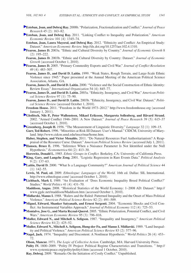
1341EsTEBAn ET AL.: EThniciTy And confLicT: An EmpiRicAL sTudyVoL. 102 no. 4
Esteban, Joan, and Debraj Ray. 2008b. “Polarization, Fractionalization and Conflict.” Journal of peace Research 45 (2): 163–82.
Esteban, Joan, and Debraj Ray. 2011. “Linking Conflict to Inequality and Polarization.” American Economic Review 101 (4): 1345–74.
Esteban, Joan, Laura Mayoral, and Debraj Ray. 2012. “Ethnicity and Conflict: An Empirical Study: Dataset.” American Economic Review. http://dx.doi.org/10.1257/aer.102.4.1310.
Fearon, James D. 2003a. “Ethnic and Cultural Diversity by Country.” Journal of Economic Growth 8 (2): 195–222.
Fearon, James D. 2003b. “Ethnic and Cultural Diversity by Country: Dataset.” Journal of Economic Growth (accessed October 1, 2010).
Fearon, James D. 2005. “Primary Commodity Exports and Civil War.” Journal of conflict Resolution 49 (4): 483–507.
Fearon, James D., and David D. Laitin. 1999. “Weak States, Rough Terrain, and Large-Scale Ethnic Violence since 1945.” Paper presented at the Annual Meeting of the American Political Science Association, Atlanta, GA.
Fearon, James D., and David D. Laitin. 2000. “Violence and the Social Construction of Ethnic Identity: Review Essay.” international organization 54 (4): 845–77.
Fearon, James D., and David D. Laitin. 2003a. “Ethnicity, Insurgency, and Civil War.” American politi-cal science Review 97 (1): 75–90.
Fearon, James D., and David D. Laitin. 2003b. “Ethnicity, Insurgency, and Civil War: Dataset.” politi-cal science Review (accessed October 1, 2010).
Freedom House. 2011. “Freedom in the World 1973–2012.” http://www.freedomhouse.org (accessed January 1, 2011).
Gleditsch, Nils P., Peter Wallensteen, Mikael Eriksson, Margareta Sollenberg, and Håvard Strand. 2002. “Armed Conflict 1946–2001: A New Dataset.” Journal of peace Research 39 (5): 615–37 (accessed October 1, 2010).
Greenberg, Joseph H. 1956. “The Measurement of Linguistic Diversity.” Language 32 (1): 109–15.Gurr, Ted Robert. 1996. “Minorities at Risk III Dataset: User’s Manual.” CIDCM, University of Mary-
land. http://www.cidcm.umd.edu/inscr/mar/home.htm.Haber, Stephen, and Victor Menaldo. 2011. “Do Natural Resources Fuel Authoritarianism? A Reap-
praisal of the Resource Curse: Dataset.” American political science Review (accessed July 1, 2011). Hansen, Bruce E. 1996. “Inference When a Nuisance Parameter Is Not Identified under the Null
Hypothesis.” Econometrica 64 (2): 413–30.Horowitz, Donald L. 1985. Ethnic Groups in conflict. Berkeley, CA: University of California Press.King, Gary, and Langche Zeng. 2001. “Logistic Regression in Rare Events Data.” political Analysis
9 (2): 137–63.Laitin, David D. 2000. “What Is a Language Community?” American Journal of political science 44
(1): 142–55.Lewis, M. Paul, ed. 2009. Ethnologue: Languages of the World. 16th ed. Dallas: SIL International.
http://www.ethnologue.com/ (accessed October 1, 2010).Lichbach, Mark I. 1989. “An Evaluation of ‘Does Economic Inequality Breed Political Conflict?’
Studies.” World politics 41 (4): 431–70.Maddison, Angus. 2008. “Historical Statistics of the World Economy: 1–2008 AD: Dataset.” http://
www.ggdc.net/maddison/Maddison.htm (accessed October 1, 2010).Midlarski, Manus I. 1988. “Rulers and the Ruled: Patterned Inequality and the Onset of Mass Political
Violence.” American political science Review 82 (2): 491–509.Miguel, Edward, Shanker Satyanath, and Ernest Sergenti. 2004. “Economic Shocks and Civil Con-
flict: An Instrumental Variables Approach.” Journal of political Economy 112 (4): 725–53.Montalvo, Jose G., and Marta Reynal-Querol. 2005. “Ethnic Polarization, Potential Conflict, and Civil
Wars.” American Economic Review 95 (3): 796–816.Muller, Edward N., and Mitchell A. Seligson. 1987. “Inequality and Insurgency.” American political
science Review 81(2): 425–52.Muller, Edward N., Mitchell A. Seligson, Hung-der Fu, and Manus I. Midlarski. 1989. “Land Inequal-
ity and Political Violence.” American political science Review 83 (2): 577–96.Nagel, Jack. 1974. “Inequality and Discontent: A Nonlinear Hypothesis.” World politics 26 (4): 453–
72.Olson, Mancur. 1971. The Logic of collective Action. Cambridge, MA: Harvard University Press.Polity IV. 1800–2009. “Polity IV Project: Political Regime Characteristics and Transitions. ” http://
www.systemicpeace.org/polity/polity4.htm (accessed 1 October, 2010).Ray, Debraj. 2009. “Remarks On the Initiation of Costly Conflict.” Unpublished.
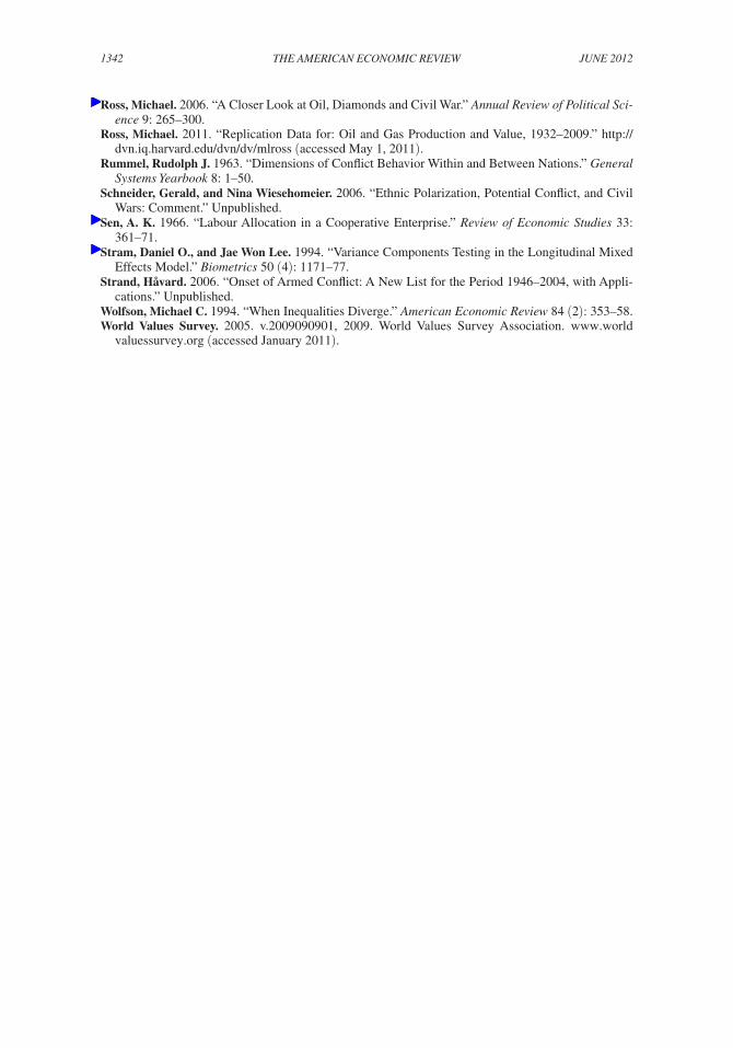
1342 ThE AmERicAn Economic REViEW JunE 2012
Ross, Michael. 2006. “A Closer Look at Oil, Diamonds and Civil War.” Annual Review of political sci-ence 9: 265–300.
Ross, Michael. 2011. “Replication Data for: Oil and Gas Production and Value, 1932–2009.” http://dvn.iq.harvard.edu/dvn/dv/mlross (accessed May 1, 2011).
Rummel, Rudolph J. 1963. “Dimensions of Conflict Behavior Within and Between Nations.” General systems yearbook 8: 1–50.
Schneider, Gerald, and Nina Wiesehomeier. 2006. “Ethnic Polarization, Potential Conflict, and Civil Wars: Comment.” Unpublished.
Sen, A. K. 1966. “Labour Allocation in a Cooperative Enterprise.” Review of Economic studies 33: 361–71.
Stram, Daniel O., and Jae Won Lee. 1994. “Variance Components Testing in the Longitudinal Mixed Effects Model.” Biometrics 50 (4): 1171–77.
Strand, Håvard. 2006. “Onset of Armed Conflict: A New List for the Period 1946–2004, with Appli-cations.” Unpublished.
Wolfson, Michael C. 1994. “When Inequalities Diverge.” American Economic Review 84 (2): 353–58.World Values Survey. 2005. v.2009090901, 2009. World Values Survey Association. www.world
valuessurvey.org (accessed January 2011).