Embed Size (px)
Citation preview
ETACE Virtual ApplianceUser Manual
Gregor Bohl, Philipp Harting, Sander van der Hoog, Bielefeld UniversityChair for Economic Theory and Computational Economics (ETACE)February 21, 2017
Contents
1 Purpose and Overview . . . . . . . . . . . . . . . . . . . . . . . . . . . . . . . . . 22 Programmes, Documentation and the Eurace@Unibi Model . . . . . . . . . . . . 23 Performance and the Linux system . . . . . . . . . . . . . . . . . . . . . . . . . . 24 Quick Starter Guide . . . . . . . . . . . . . . . . . . . . . . . . . . . . . . . . . . 35 How to use the Simulation GUI for customized Simulation Experiments . . . . . 56 Flame Modeling Environment . . . . . . . . . . . . . . . . . . . . . . . . . . . . . 237 Licensing . . . . . . . . . . . . . . . . . . . . . . . . . . . . . . . . . . . . . . . . 25
1
1 Purpose and Overview 2
1 Purpose and Overview
This User Manual for the ETACE Virtual Appliance describes how to conduct economic analy-ses with the Eurace@Unibi model using the programmes available on the VA and its respectivetools, with regard to the general workflow of the Flexible Large-scale Agent-based ModellingEnvironment (FLAME1).
The virtual appliance has been created at ETACE, the Chair for Economic Theory andComputational Economics, at Bielefeld University. The intention behind this software collectionis to make every step related to the initialization, execution, modification and analysis of theEurace@Unibi agent-based simulation model as easy as possible. We hence address here theissue of reproducibility of simulation-based research (Stodden, 2010).
2 Programmes, Documentation and the Eurace@Unibi Model
This software package is based on the SliTaz distribution of free software, that includes theLinux kernel. The coresponding documentation is included in the software.
Programs provided in the Virtual Appliance (including their dependencies):
Xparser GUI : Parser for FLAME models.GNU GCC compiler : C compiler for model + framework code.Flame Editor : Generate model.xml file, XML description of model.Population GUI : Generates initialization files, population description.Simulation GUI : Settings for simulation experiments and data analysis.
Apart from standard dependencies such as GNU GCC, the relevant documentation to theseprogrammes can be found in the Documentation folder on the Desktop.
The following versions of the Eurace@Unibi model are included and can be found in theModels folder on the Desktop:
Dawid et al., 2011 : full source code of Eurace@Unibi 1.0Dawid and Gemkow, 2013 : main, model.xml, 0.pop & 0.xml for reproductionDawid et al., 2014b : full source code of the model used for the paperDawid et al., 2014a : full source code of the model used for the paper
For the following papers, a pre-configured ready-to-run experiment can be found in the./Preconfigured Experiments folder:
Dawid et al., 2014a : ./Preconfigured Experiments/WP Dawid Harting Neugart 2014/
3 Performance and the Linux system
The virtual appliance is set up with a minimum performance configuration. You can increasethe performance of the VA especially by increasing the number of processors and the size of theallocated memory. However, the performance is limited by the configuration of the host system.To change these:
1 http://www.flame.ac.uk/
4 Quick Starter Guide 3
• Enable hardware virtualization support in your own system’s BIOS to run in multi-core mode (normally under menu ”CPU” in BIOS).
• In the settings of the virtual machine itself (i.e. in the client of Oracle’s VirtualBox butnot inside this virtual appliance), you can change the number of assigned CPU cores andRAM memory.
The default memory size allocated to the VA might not be sufficient for the post-processing of large simulations with big data bases. In this case, in order to suc-cessfully finish the R processes that read the data and generate the plots of thesimulations, it can be necessary to increase the size of the allocated memory.
To get root access in a terminal, type su with password root. The Super User is likewiseroot with password root. All the relevant files have been placed on the Desktop (/home/eurace/Desktop), whereas additional libraries (Libmboard, R, Python, GSL) have been installed directlyinto the system.
There is also the possibility to mount a shared folder in order to facilitate the exchange offiles between the VA and the host system. A separate instruction how to mount a shared foldercan be found on the dedicated webpage of the VA.
4 Quick Starter Guide
The Desktop
After launching, you should see the desktop of the VA. The desktop contains folders and programlaunchers. The folders are• Documentation; this folder contains the licenses of the ETACE
Virtual Appliance, as well as manuals for GUIs and applicationsused in the VA. Furthermore, it contains a description of the Eu-race@Unibi model together with several research papers based onthe model.
• src; this folder contains source files of applications.
• Models; this folder hosts source code and executables of differentversions of the Eurace@Unibi model.
• exper; this is an empty folder for storing new simulation experi-ments of the user.
• Preconfigured Experiments; this folder contains ready-to-run simu-lation setups for exact paper reproduction.
The launchers can be used to launch different GUIs:
• PopulationGUI; to create an initial state as input of a simulation.
4 Quick Starter Guide 4
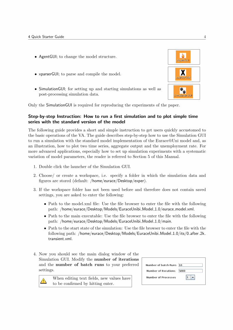
• AgentGUI; to change the model structure.
• xparserGUI; to parse and compile the model.
• SimulationGUI; for setting up and starting simulations as well aspost-processing simulation data.
Only the SimulationGUI is required for reproducing the experiments of the paper.
Step-by-step Instruction: How to run a first simulation and to plot simple timeseries with the standard version of the model
The following guide provides a short and simple instruction to get users quickly accustomed tothe basic operations of the VA. The guide describes step-by-step how to use the Simulation GUIto run a simulation with the standard model implementation of the Eurace@Uni model and, asan illustration, how to plot two time series, aggregate output and the unemployment rate. Formore advanced applications, especially how to set up simulation experiments with a systematicvariation of model parameters, the reader is referred to Section 5 of this Manual.
1. Double click the launcher of the Simulation GUI.
2. Choose/ or create a workspace, i.e. specify a folder in which the simulation data andfigures are stored (default: /home/eurace/Desktop/exper).
3. If the workspace folder has not been used before and therefore does not contain savedsettings, you are asked to enter the following:
• Path to the model.xml file: Use the file browser to enter the file with the followingpath: /home/eurace/Desktop/Models/EuraceUnibi Model 1.0/eurace model.xml.
• Path to the main executable: Use the file browser to enter the file with the followingpath: /home/eurace/Desktop/Models/EuraceUnibi Model 1.0/main.
• Path to the start state of the simulation: Use the file browser to enter the file with thefollowing path: /home/eurace/Desktop/Models/EuraceUnibi Model 1.0/its/0 after 2ktransient.xml.
4. Now you should see the main dialog window of theSimulation GUI. Modify the number of iterationsand the number of batch runs to your preferredsettings.
When editing text fields, new values haveto be confirmed by hitting enter.
5 How to use the Simulation GUI for customized Simulation Experiments 5
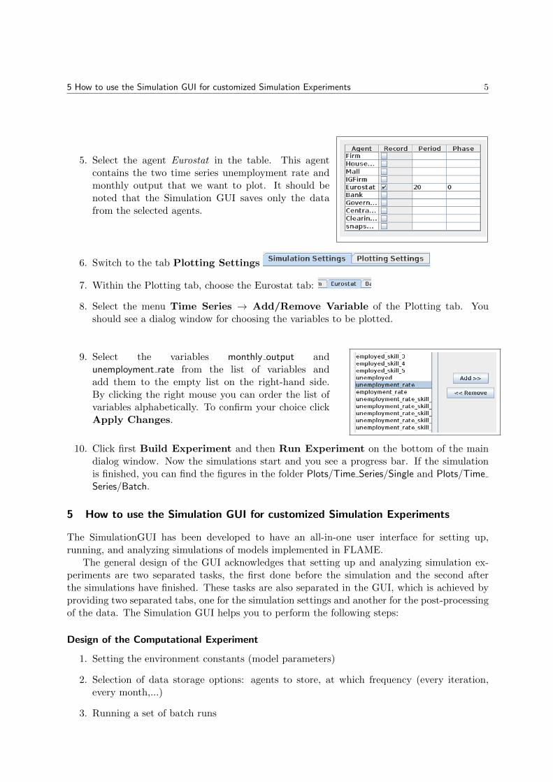
5. Select the agent Eurostat in the table. This agentcontains the two time series unemployment rate andmonthly output that we want to plot. It should benoted that the Simulation GUI saves only the datafrom the selected agents.
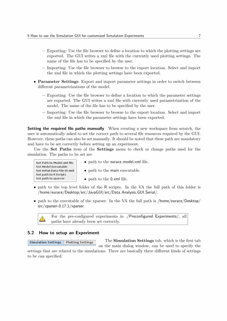
6. Switch to the tab Plotting Settings
7. Within the Plotting tab, choose the Eurostat tab:
8. Select the menu Time Series → Add/Remove Variable of the Plotting tab. Youshould see a dialog window for choosing the variables to be plotted.
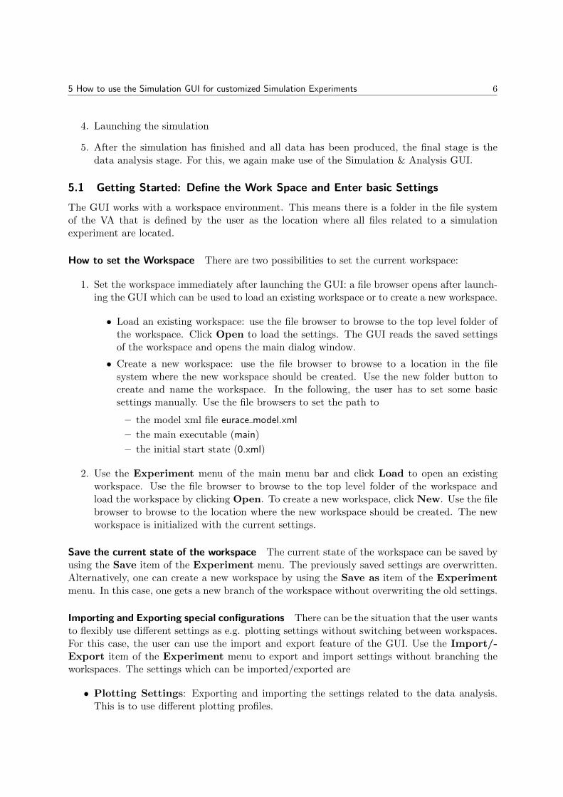
9. Select the variables monthly output andunemployment rate from the list of variables andadd them to the empty list on the right-hand side.By clicking the right mouse you can order the list ofvariables alphabetically. To confirm your choice clickApply Changes.
10. Click first Build Experiment and then Run Experiment on the bottom of the maindialog window. Now the simulations start and you see a progress bar. If the simulationis finished, you can find the figures in the folder Plots/Time Series/Single and Plots/TimeSeries/Batch.
5 How to use the Simulation GUI for customized Simulation Experiments
The SimulationGUI has been developed to have an all-in-one user interface for setting up,running, and analyzing simulations of models implemented in FLAME.
The general design of the GUI acknowledges that setting up and analyzing simulation ex-periments are two separated tasks, the first done before the simulation and the second afterthe simulations have finished. These tasks are also separated in the GUI, which is achieved byproviding two separated tabs, one for the simulation settings and another for the post-processingof the data. The Simulation GUI helps you to perform the following steps:
Design of the Computational Experiment
1. Setting the environment constants (model parameters)
2. Selection of data storage options: agents to store, at which frequency (every iteration,every month,...)
3. Running a set of batch runs
5 How to use the Simulation GUI for customized Simulation Experiments 6
4. Launching the simulation
5. After the simulation has finished and all data has been produced, the final stage is thedata analysis stage. For this, we again make use of the Simulation & Analysis GUI.
5.1 Getting Started: Define the Work Space and Enter basic Settings
The GUI works with a workspace environment. This means there is a folder in the file systemof the VA that is defined by the user as the location where all files related to a simulationexperiment are located.
How to set the Workspace There are two possibilities to set the current workspace:
1. Set the workspace immediately after launching the GUI: a file browser opens after launch-ing the GUI which can be used to load an existing workspace or to create a new workspace.
• Load an existing workspace: use the file browser to browse to the top level folder ofthe workspace. Click Open to load the settings. The GUI reads the saved settingsof the workspace and opens the main dialog window.
• Create a new workspace: use the file browser to browse to a location in the filesystem where the new workspace should be created. Use the new folder button tocreate and name the workspace. In the following, the user has to set some basicsettings manually. Use the file browsers to set the path to
– the model xml file eurace model.xml
– the main executable (main)
– the initial start state (0.xml)
2. Use the Experiment menu of the main menu bar and click Load to open an existingworkspace. Use the file browser to browse to the top level folder of the workspace andload the workspace by clicking Open. To create a new workspace, click New. Use the filebrowser to browse to the location where the new workspace should be created. The newworkspace is initialized with the current settings.
Save the current state of the workspace The current state of the workspace can be saved byusing the Save item of the Experiment menu. The previously saved settings are overwritten.Alternatively, one can create a new workspace by using the Save as item of the Experimentmenu. In this case, one gets a new branch of the workspace without overwriting the old settings.
Importing and Exporting special configurations There can be the situation that the user wantsto flexibly use different settings as e.g. plotting settings without switching between workspaces.For this case, the user can use the import and export feature of the GUI. Use the Import/-Export item of the Experiment menu to export and import settings without branching theworkspaces. The settings which can be imported/exported are
• Plotting Settings: Exporting and importing the settings related to the data analysis.This is to use different plotting profiles.
5 How to use the Simulation GUI for customized Simulation Experiments 7
– Exporting: Use the file browser to define a location to which the plotting settings areexported. The GUI writes a xml file with the currently used plotting settings. Thename of the file has to be specified by the user.
– Importing: Use the file browser to browse to the export location. Select and importthe xml file in which the plotting settings have been exported.
• Parameter Settings: Export and import parameter settings in order to switch betweendifferent parametrizations of the model.
– Exporting: Use the file browser to define a location to which the parameter settingsare exported. The GUI writes a xml file with currently used parametrization of themodel. The name of the file has to be specified by the user.
– Importing: Use the file browser to browse to the export location. Select and importthe xml file in which the parameter settings have been exported.
Setting the required file paths manually When creating a new workspace from scratch, theuser is automatically asked to set the correct path to several file resources required by the GUI.However, these paths can also be set manually. It should be noted that these path are mandatoryand have to be set correctly before setting up an experiment.
Use the Set Paths item of the Settings menu to check or change paths used for thesimulation. The paths to be set are
• path to the eurace model.xml file.
• path to the main executable.
• path to the 0.xml file.
• path to the top level folder of the R scripts. In the VA the full path of this folder is/home/eurace/Desktop/src/JavaGUI/src/Data Analysis GUI Serial/.
• path to the executable of the xparser. In the VA the full path is /home/eurace/Desktop/src/xparser-0.17.1/xparser.
For the pre-configured experiments in ./Preconfigured Experiments/, allpaths have already been set correctly.
5.2 How to setup an Experiment
The Simulation Settings tab, which is the first tabon the main dialog window, can be used to specify the
settings that are related to the simulations. There are basically three different kinds of settingsto be can specified:
5 How to use the Simulation GUI for customized Simulation Experiments 8
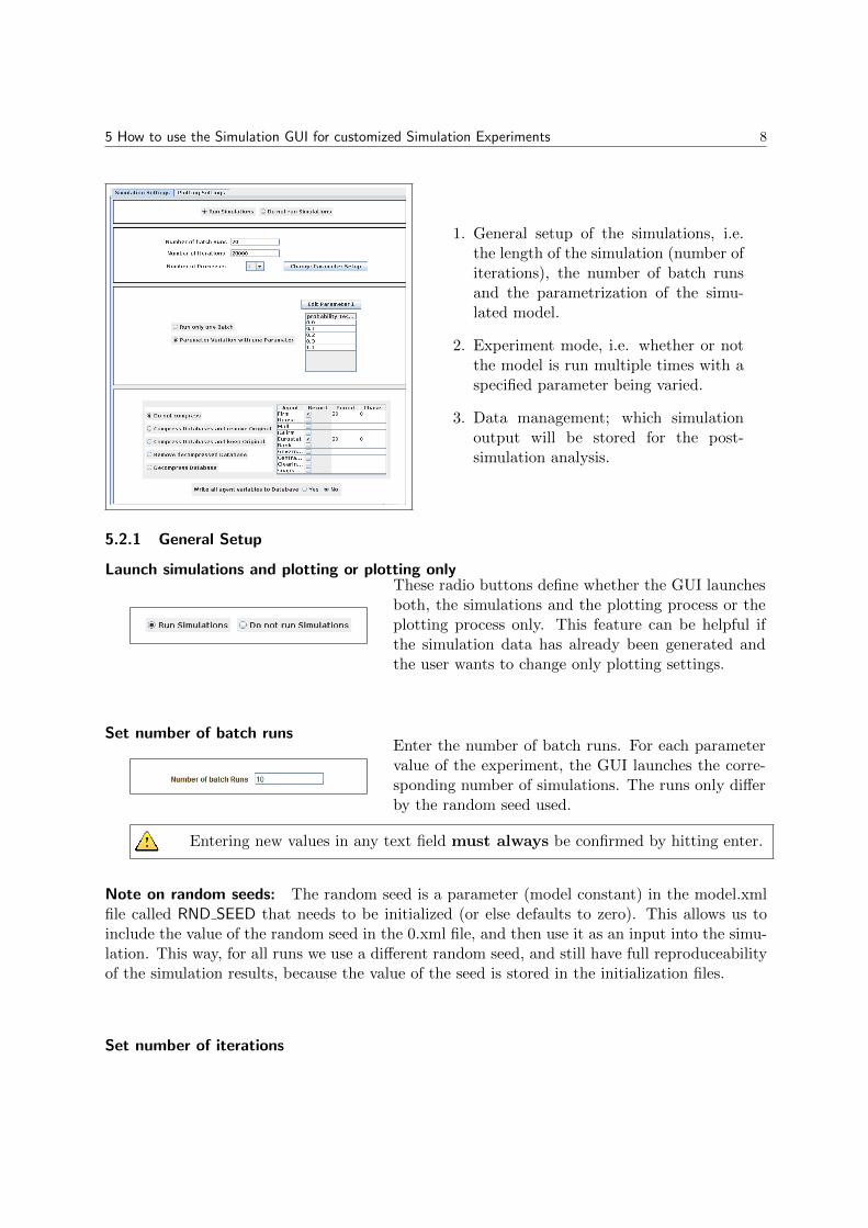
1. General setup of the simulations, i.e.the length of the simulation (number ofiterations), the number of batch runsand the parametrization of the simu-lated model.
2. Experiment mode, i.e. whether or notthe model is run multiple times with aspecified parameter being varied.
3. Data management; which simulationoutput will be stored for the post-simulation analysis.
5.2.1 General Setup
Launch simulations and plotting or plotting onlyThese radio buttons define whether the GUI launchesboth, the simulations and the plotting process or theplotting process only. This feature can be helpful ifthe simulation data has already been generated andthe user wants to change only plotting settings.
Set number of batch runsEnter the number of batch runs. For each parametervalue of the experiment, the GUI launches the corre-sponding number of simulations. The runs only differby the random seed used.
Entering new values in any text field must always be confirmed by hitting enter.
Note on random seeds: The random seed is a parameter (model constant) in the model.xmlfile called RND SEED that needs to be initialized (or else defaults to zero). This allows us toinclude the value of the random seed in the 0.xml file, and then use it as an input into the simu-lation. This way, for all runs we use a different random seed, and still have full reproduceabilityof the simulation results, because the value of the seed is stored in the initialization files.
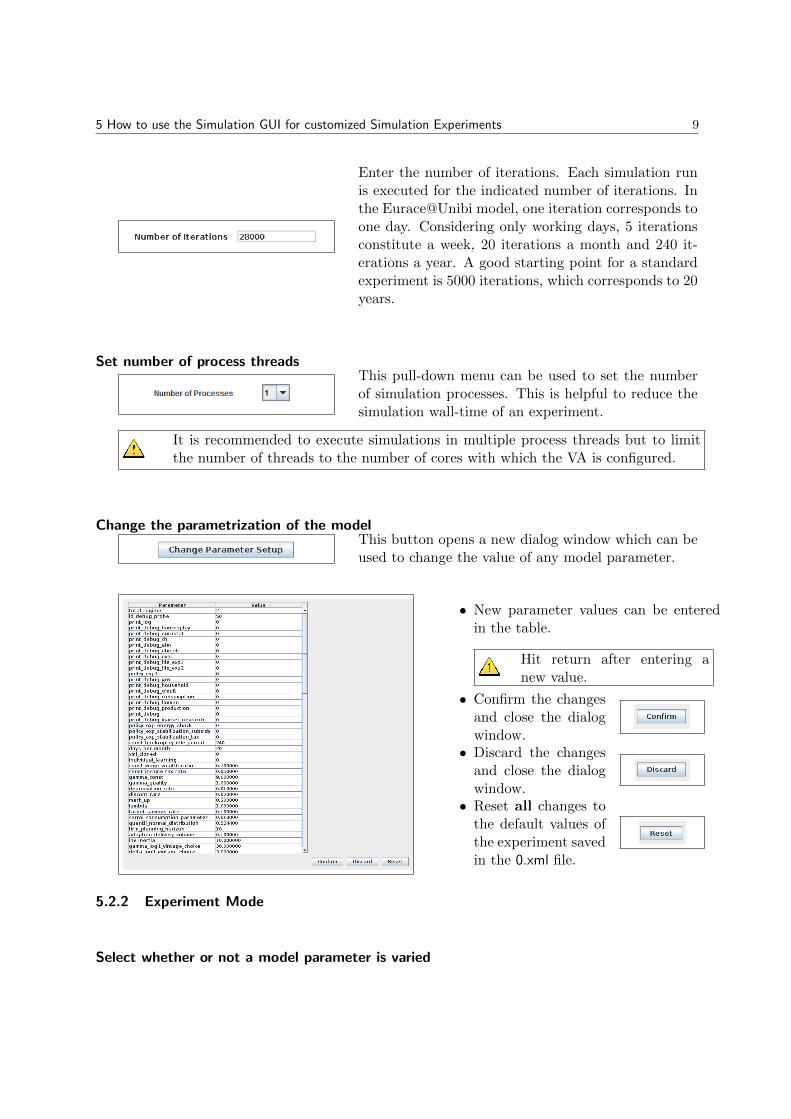
Set number of iterations
5 How to use the Simulation GUI for customized Simulation Experiments 9
Enter the number of iterations. Each simulation runis executed for the indicated number of iterations. Inthe Eurace@Unibi model, one iteration corresponds toone day. Considering only working days, 5 iterationsconstitute a week, 20 iterations a month and 240 it-erations a year. A good starting point for a standardexperiment is 5000 iterations, which corresponds to 20years.
Set number of process threadsThis pull-down menu can be used to set the numberof simulation processes. This is helpful to reduce thesimulation wall-time of an experiment.
It is recommended to execute simulations in multiple process threads but to limitthe number of threads to the number of cores with which the VA is configured.
Change the parametrization of the modelThis button opens a new dialog window which can beused to change the value of any model parameter.
• New parameter values can be enteredin the table.
Hit return after entering anew value.
• Confirm the changesand close the dialogwindow.• Discard the changes
and close the dialogwindow.• Reset all changes to
the default values ofthe experiment savedin the 0.xml file.
5.2.2 Experiment Mode
Select whether or not a model parameter is varied
5 How to use the Simulation GUI for customized Simulation Experiments 10
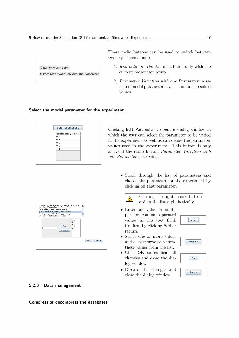
These radio buttons can be used to switch betweentwo experiment modes:
1. Run only one Batch: run a batch only with thecurrent parameter setup.
2. Parameter Variation with one Parameter : a se-lected model parameter is varied among specifiedvalues
Select the model parameter for the experiment
Clicking Edit Parameter 1 opens a dialog window inwhich the user can select the parameter to be variedin the experiment as well as can define the parametervalues used in the experiment. This button is onlyactive if the radio button Parameter Variation withone Parameter is selected.
• Scroll through the list of parameters andchoose the parameter for the experiment byclicking on that parameter.
Clicking the right mouse buttonorders the list alphabetically.
• Enter one value or multi-ple, by comma separatedvalues in the text field.Confirm by clicking Add orreturn.• Select one or more values
and click remove to removethese values from the list.• Click OK to confirm all
changes and close the dia-log window.
• Discard the changes andclose the dialog window.
5.2.3 Data management
Compress or decompress the databases
5 How to use the Simulation GUI for customized Simulation Experiments 11
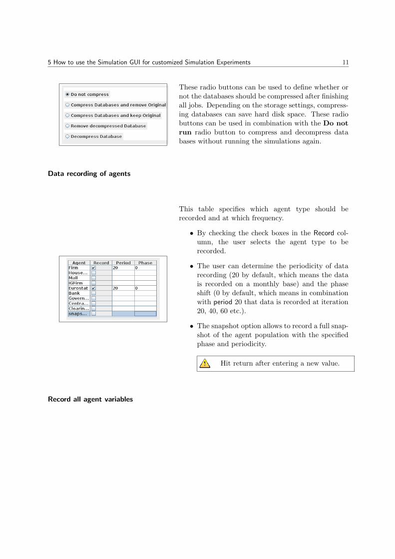
These radio buttons can be used to define whether ornot the databases should be compressed after finishingall jobs. Depending on the storage settings, compress-ing databases can save hard disk space. These radiobuttons can be used in combination with the Do notrun radio button to compress and decompress databases without running the simulations again.
Data recording of agents
This table specifies which agent type should berecorded and at which frequency.
• By checking the check boxes in the Record col-umn, the user selects the agent type to berecorded.
• The user can determine the periodicity of datarecording (20 by default, which means the datais recorded on a monthly base) and the phaseshift (0 by default, which means in combinationwith period 20 that data is recorded at iteration20, 40, 60 etc.).
• The snapshot option allows to record a full snap-shot of the agent population with the specifiedphase and periodicity.
Hit return after entering a new value.
Record all agent variables
5 How to use the Simulation GUI for customized Simulation Experiments 12
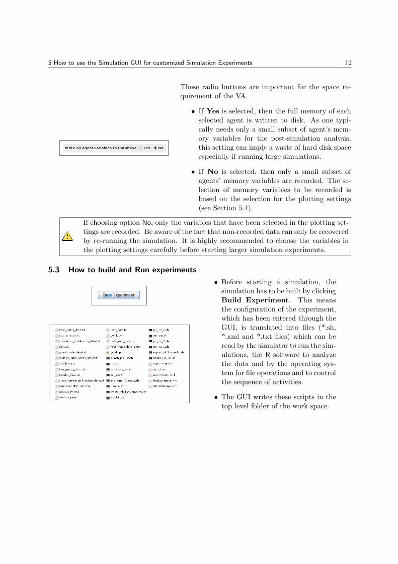
These radio buttons are important for the space re-quirement of the VA.
• If Yes is selected, then the full memory of eachselected agent is written to disk. As one typi-cally needs only a small subset of agent’s mem-ory variables for the post-simulation analysis,this setting can imply a waste of hard disk spaceespecially if running large simulations.
• If No is selected, then only a small subset ofagents’ memory variables are recorded. The se-lection of memory variables to be recorded isbased on the selection for the plotting settings(see Section 5.4).
If choosing option No, only the variables that have been selected in the plotting set-tings are recorded. Be aware of the fact that non-recorded data can only be recoveredby re-running the simulation. It is highly recommended to choose the variables inthe plotting settings carefully before starting larger simulation experiments.
5.3 How to build and Run experiments
• Before starting a simulation, thesimulation has to be built by clickingBuild Experiment. This meansthe configuration of the experiment,which has been entered through theGUI, is translated into files (*.sh,*.xml and *.txt files) which can beread by the simulator to run the sim-ulations, the R software to analyzethe data and by the operating sys-tem for file operations and to controlthe sequence of activities.
• The GUI writes these scripts in thetop level folder of the work space.
5 How to use the Simulation GUI for customized Simulation Experiments 13
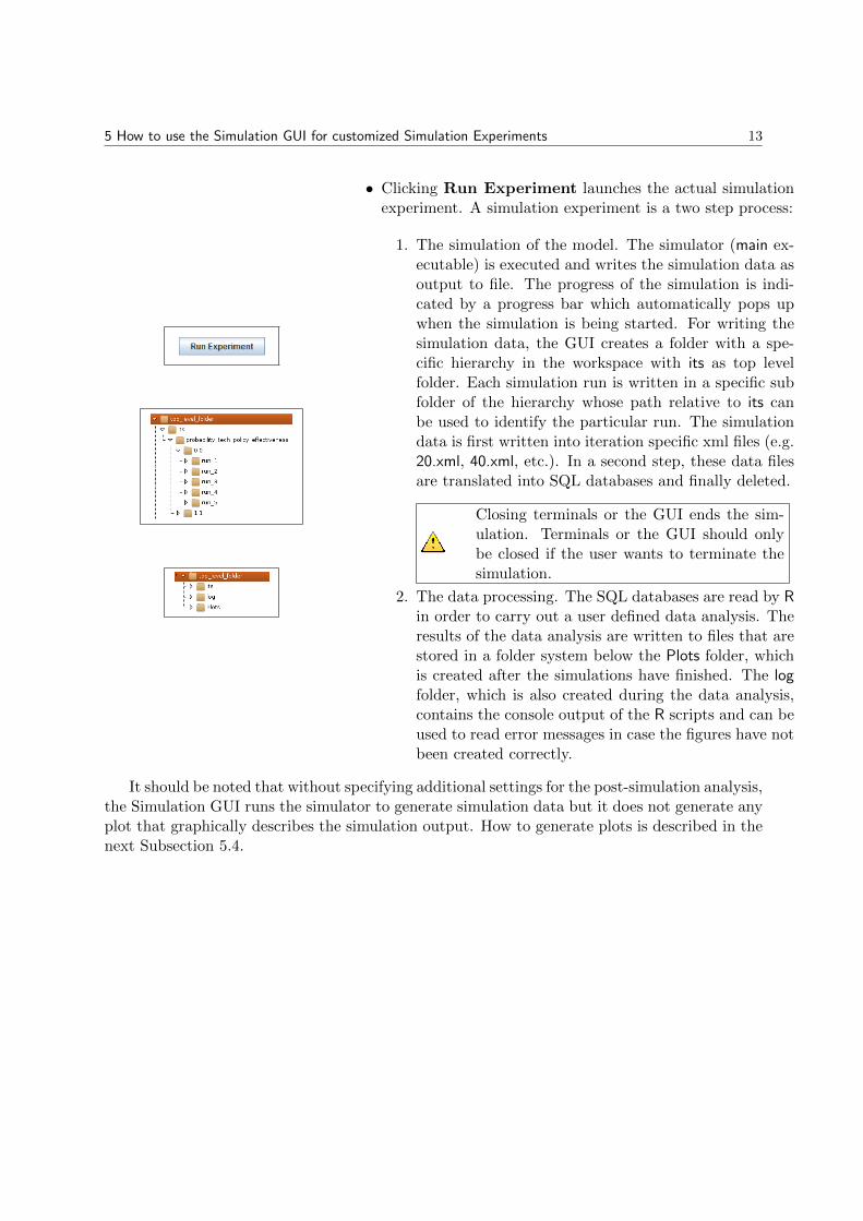
• Clicking Run Experiment launches the actual simulationexperiment. A simulation experiment is a two step process:
1. The simulation of the model. The simulator (main ex-ecutable) is executed and writes the simulation data asoutput to file. The progress of the simulation is indi-cated by a progress bar which automatically pops upwhen the simulation is being started. For writing thesimulation data, the GUI creates a folder with a spe-cific hierarchy in the workspace with its as top levelfolder. Each simulation run is written in a specific subfolder of the hierarchy whose path relative to its canbe used to identify the particular run. The simulationdata is first written into iteration specific xml files (e.g.20.xml, 40.xml, etc.). In a second step, these data filesare translated into SQL databases and finally deleted.
Closing terminals or the GUI ends the sim-ulation. Terminals or the GUI should onlybe closed if the user wants to terminate thesimulation.
2. The data processing. The SQL databases are read by Rin order to carry out a user defined data analysis. Theresults of the data analysis are written to files that arestored in a folder system below the Plots folder, whichis created after the simulations have finished. The logfolder, which is also created during the data analysis,contains the console output of the R scripts and can beused to read error messages in case the figures have notbeen created correctly.
It should be noted that without specifying additional settings for the post-simulation analysis,the Simulation GUI runs the simulator to generate simulation data but it does not generate anyplot that graphically describes the simulation output. How to generate plots is described in thenext Subsection 5.4.
5 How to use the Simulation GUI for customized Simulation Experiments 14
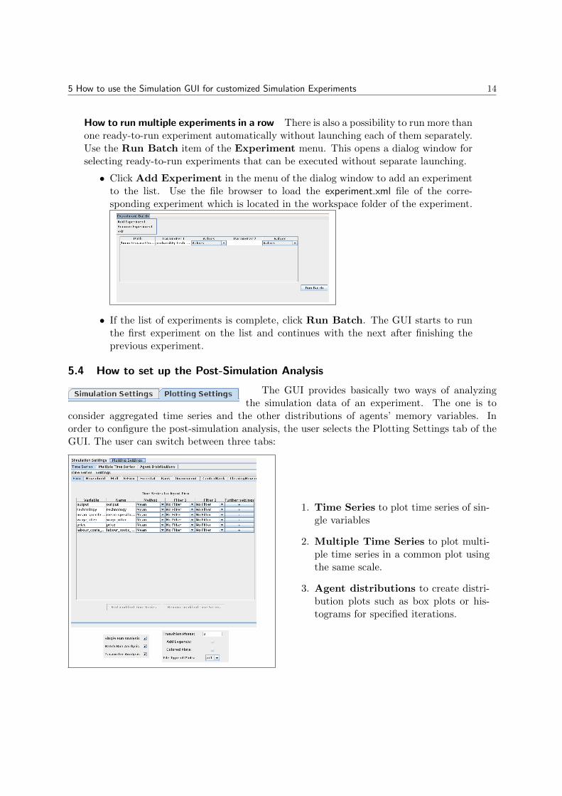
How to run multiple experiments in a row There is also a possibility to run more thanone ready-to-run experiment automatically without launching each of them separately.Use the Run Batch item of the Experiment menu. This opens a dialog window forselecting ready-to-run experiments that can be executed without separate launching.
• Click Add Experiment in the menu of the dialog window to add an experimentto the list. Use the file browser to load the experiment.xml file of the corre-sponding experiment which is located in the workspace folder of the experiment.
• If the list of experiments is complete, click Run Batch. The GUI starts to runthe first experiment on the list and continues with the next after finishing theprevious experiment.
5.4 How to set up the Post-Simulation Analysis
The GUI provides basically two ways of analyzingthe simulation data of an experiment. The one is to
consider aggregated time series and the other distributions of agents’ memory variables. Inorder to configure the post-simulation analysis, the user selects the Plotting Settings tab of theGUI. The user can switch between three tabs:
1. Time Series to plot time series of sin-gle variables
2. Multiple Time Series to plot multi-ple time series in a common plot usingthe same scale.
3. Agent distributions to create distri-bution plots such as box plots or his-tograms for specified iterations.
5 How to use the Simulation GUI for customized Simulation Experiments 15
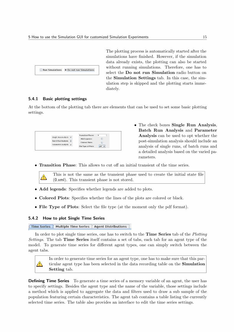
The plotting process is automatically started after thesimulations have finished. However, if the simulationdata already exists, the plotting can also be startedwithout running simulations. Therefore, one has toselect the Do not run Simulation radio button onthe Simulation Settings tab. In this case, the sim-ulation step is skipped and the plotting starts imme-diately.
5.4.1 Basic plotting settings
At the bottom of the plotting tab there are elements that can be used to set some basic plottingsettings.
• The check boxes Single Run Analysis,Batch Run Analysis and ParameterAnalysis can be used to opt whether thepost-simulation analysis should include ananalysis of single runs, of batch runs anda detailed analysis based on the varied pa-rameters.
• Transition Phase: This allows to cut off an initial transient of the time series.
This is not the same as the transient phase used to create the initial state file(0.xml). This transient phase is not stored.
• Add legends: Specifies whether legends are added to plots.
• Colored Plots: Specifies whether the lines of the plots are colored or black.
• File Type of Plots: Select the file type (at the moment only the pdf format).
5.4.2 How to plot Single Time Series
In order to plot single time series, one has to switch to the Time Series tab of the PlottingSettings. The tab Time Series itself contains a set of tabs, each tab for an agent type of themodel. To generate time series for different agent types, one can simply switch between theagent tabs.
In order to generate time series for an agent type, one has to make sure that this par-ticular agent type has been selected in the data recording table on the SimulationSetting tab.
Defining Time Series To generate a time series of a memory variable of an agent, the user hasto specify settings. Besides the agent type and the name of the variable, those settings includea method which is applied to aggregate the data and filters used to draw a sub sample of thepopulation featuring certain characteristics. The agent tab contains a table listing the currentlyselected time series. The table also provides an interface to edit the time series settings.
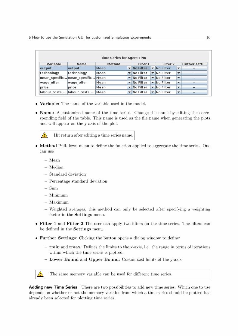
5 How to use the Simulation GUI for customized Simulation Experiments 16
• Variable: The name of the variable used in the model.
• Name: A customized name of the time series. Change the name by editing the corre-sponding field of the table. This name is used as the file name when generating the plotsand will appear on the y-axis of the plot.
Hit return after editing a time series name.
• Method Pull-down menu to define the function applied to aggregate the time series. Onecan use
– Mean
– Median
– Standard deviation
– Percentage standard deviation
– Sum
– Minimum
– Maximum
– Weighted averages; this method can only be selected after specifying a weightingfactor in the Settings menu.
• Filter 1 and Filter 2 The user can apply two filters on the time series. The filters canbe defined in the Settings menu.
• Further Settings: Clicking the button opens a dialog window to define:
– tmin and tmax: Defines the limits to the x-axis, i.e. the range in terms of iterationswithin which the time series is plotted.
– Lower Bound and Upper Bound: Customized limits of the y-axis.
The same memory variable can be used for different time series.
Adding new Time Series There are two possibilities to add new time series. Which one to usedepends on whether or not the memory variable from which a time series should be plotted hasalready been selected for plotting time series.
5 How to use the Simulation GUI for customized Simulation Experiments 17
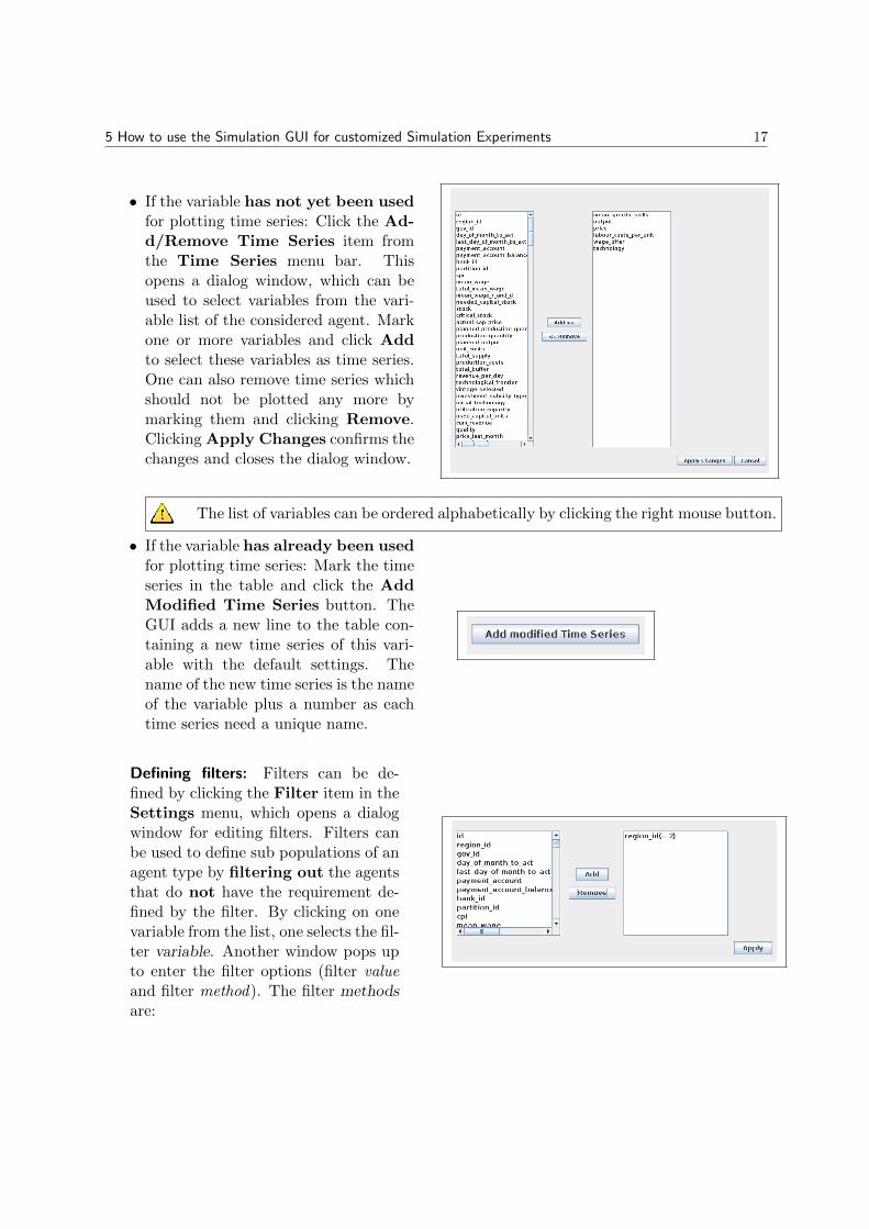
• If the variable has not yet been usedfor plotting time series: Click the Ad-d/Remove Time Series item fromthe Time Series menu bar. Thisopens a dialog window, which can beused to select variables from the vari-able list of the considered agent. Markone or more variables and click Addto select these variables as time series.One can also remove time series whichshould not be plotted any more bymarking them and clicking Remove.Clicking Apply Changes confirms thechanges and closes the dialog window.
The list of variables can be ordered alphabetically by clicking the right mouse button.
• If the variable has already been usedfor plotting time series: Mark the timeseries in the table and click the AddModified Time Series button. TheGUI adds a new line to the table con-taining a new time series of this vari-able with the default settings. Thename of the new time series is the nameof the variable plus a number as eachtime series need a unique name.
Defining filters: Filters can be de-fined by clicking the Filter item in theSettings menu, which opens a dialogwindow for editing filters. Filters canbe used to define sub populations of anagent type by filtering out the agentsthat do not have the requirement de-fined by the filter. By clicking on onevariable from the list, one selects the fil-ter variable. Another window pops upto enter the filter options (filter valueand filter method). The filter methodsare:
5 How to use the Simulation GUI for customized Simulation Experiments 18
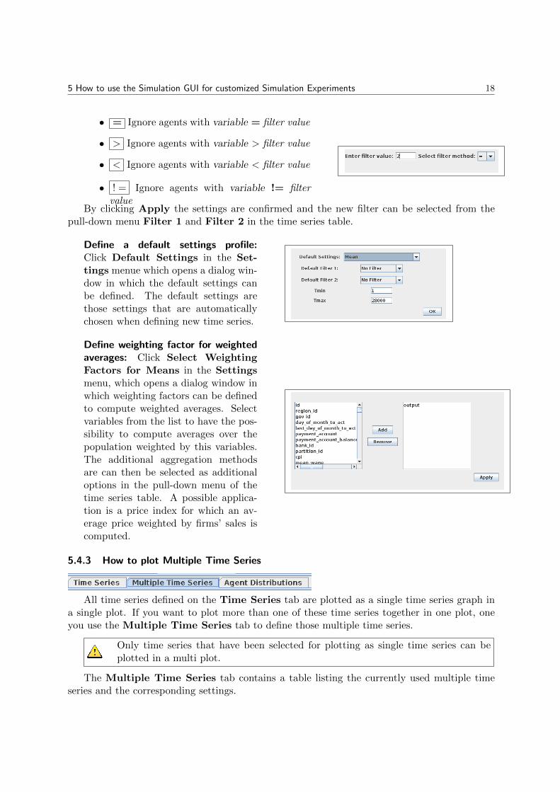
• = Ignore agents with variable = filter value
• > Ignore agents with variable > filter value
• < Ignore agents with variable < filter value
• ! = Ignore agents with variable != filtervalue
By clicking Apply the settings are confirmed and the new filter can be selected from thepull-down menu Filter 1 and Filter 2 in the time series table.
Define a default settings profile:Click Default Settings in the Set-tings menue which opens a dialog win-dow in which the default settings canbe defined. The default settings arethose settings that are automaticallychosen when defining new time series.
Define weighting factor for weightedaverages: Click Select WeightingFactors for Means in the Settingsmenu, which opens a dialog window inwhich weighting factors can be definedto compute weighted averages. Selectvariables from the list to have the pos-sibility to compute averages over thepopulation weighted by this variables.The additional aggregation methodsare can then be selected as additionaloptions in the pull-down menu of thetime series table. A possible applica-tion is a price index for which an av-erage price weighted by firms’ sales iscomputed.
5.4.3 How to plot Multiple Time Series
All time series defined on the Time Series tab are plotted as a single time series graph ina single plot. If you want to plot more than one of these time series together in one plot, oneyou use the Multiple Time Series tab to define those multiple time series.
Only time series that have been selected for plotting as single time series can beplotted in a multi plot.
The Multiple Time Series tab contains a table listing the currently used multiple timeseries and the corresponding settings.
5 How to use the Simulation GUI for customized Simulation Experiments 19
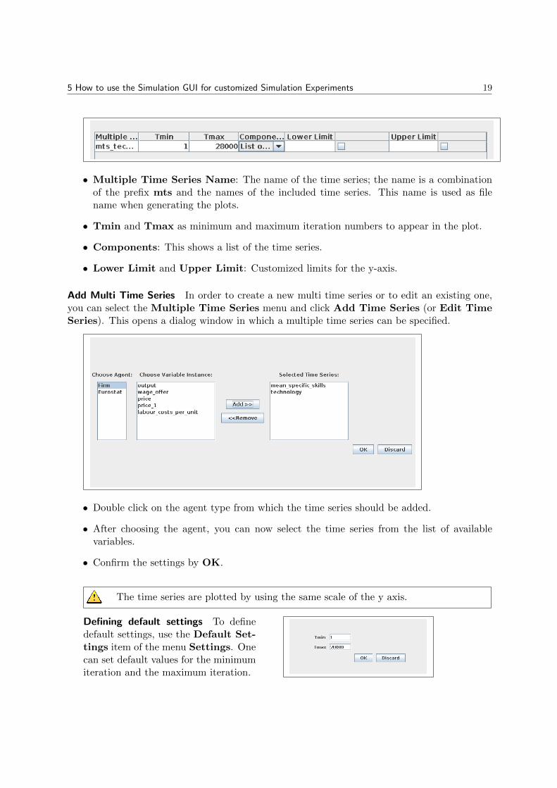
• Multiple Time Series Name: The name of the time series; the name is a combinationof the prefix mts and the names of the included time series. This name is used as filename when generating the plots.
• Tmin and Tmax as minimum and maximum iteration numbers to appear in the plot.
• Components: This shows a list of the time series.
• Lower Limit and Upper Limit: Customized limits for the y-axis.
Add Multi Time Series In order to create a new multi time series or to edit an existing one,you can select the Multiple Time Series menu and click Add Time Series (or Edit TimeSeries). This opens a dialog window in which a multiple time series can be specified.
• Double click on the agent type from which the time series should be added.
• After choosing the agent, you can now select the time series from the list of availablevariables.
• Confirm the settings by OK.
The time series are plotted by using the same scale of the y axis.
Defining default settings To definedefault settings, use the Default Set-tings item of the menu Settings. Onecan set default values for the minimumiteration and the maximum iteration.
5 How to use the Simulation GUI for customized Simulation Experiments 20
5.4.4 How to plot Agent Distributions
The Agent Distribution tab can be used to analyze the distribution of agent variables inthe population. The distribution of a variable is plotted as a box plot and as a histogram fora point in time or for a discrete sequence that has to be specified by the user. By default, thedistribution is plotted for the last iteration of the simulation.
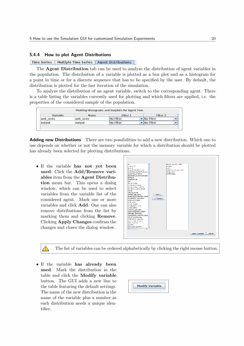
To analyze the distribution of an agent variable, switch to the corresponding agent. Thereis a table listing the variables currently used for plotting and which filters are applied, i.e. theproperties of the considered sample of the population.
Adding new Distributions There are two possibilities to add a new distribution. Which one touse depends on whether or not the memory variable for which a distribution should be plottedhas already been selected for plotting distributions.
• If the variable has not yet beenused: Click the Add/Remove vari-ables item from the Agent Distribu-tion menu bar. This opens a dialogwindow, which can be used to selectvariables from the variable list of theconsidered agent. Mark one or morevariables and click Add. One can alsoremove distributions from the list bymarking them and clicking Remove.Clicking Apply Changes confirms thechanges and closes the dialog window.
The list of variables can be ordered alphabetically by clicking the right mouse button.
• If the variable has already beenused: Mark the distribution in thetable and click the Modify variablebutton. The GUI adds a new line tothe table featuring the default settings.The name of the new distribution is thename of the variable plus a number aseach distribution needs a unique iden-tifier.
5 How to use the Simulation GUI for customized Simulation Experiments 21
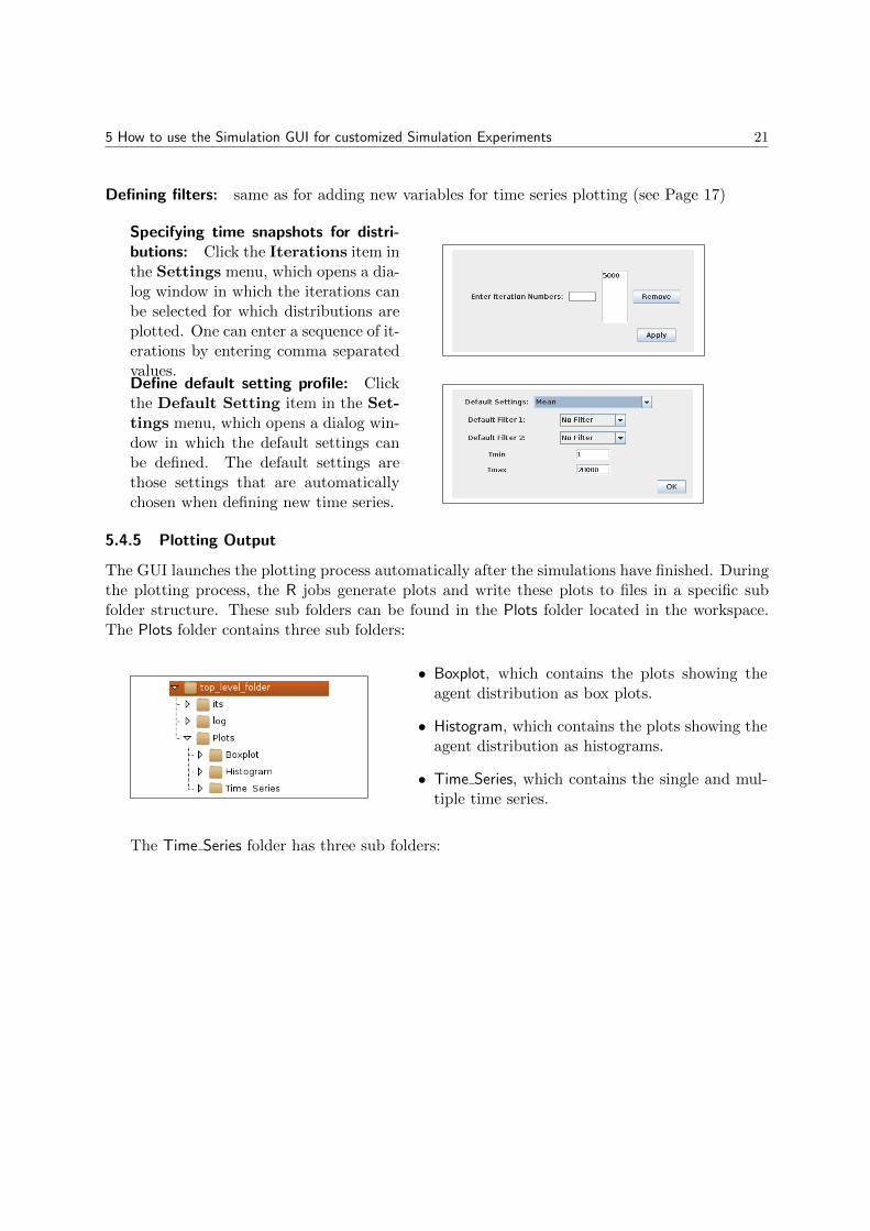
Defining filters: same as for adding new variables for time series plotting (see Page 17)
Specifying time snapshots for distri-butions: Click the Iterations item inthe Settings menu, which opens a dia-log window in which the iterations canbe selected for which distributions areplotted. One can enter a sequence of it-erations by entering comma separatedvalues.Define default setting profile: Clickthe Default Setting item in the Set-tings menu, which opens a dialog win-dow in which the default settings canbe defined. The default settings arethose settings that are automaticallychosen when defining new time series.
5.4.5 Plotting Output
The GUI launches the plotting process automatically after the simulations have finished. Duringthe plotting process, the R jobs generate plots and write these plots to files in a specific subfolder structure. These sub folders can be found in the Plots folder located in the workspace.The Plots folder contains three sub folders:
• Boxplot, which contains the plots showing theagent distribution as box plots.
• Histogram, which contains the plots showing theagent distribution as histograms.
• Time Series, which contains the single and mul-tiple time series.
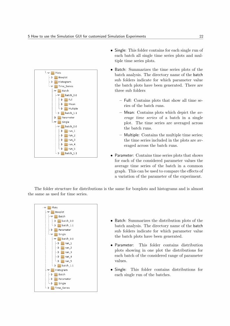
The Time Series folder has three sub folders:
5 How to use the Simulation GUI for customized Simulation Experiments 22
• Single: This folder contains for each single run ofeach batch all single time series plots and mul-tiple time series plots.
• Batch: Summarizes the time series plots of thebatch analysis. The directory name of the batchsub folders indicate for which parameter valuethe batch plots have been generated. There arethree sub folders
– Full: Contains plots that show all time se-ries of the batch runs.
– Mean: Contains plots which depict the av-erage time series of a batch in a singleplot. The time series are averaged acrossthe batch runs.
– Multiple: Contains the multiple time series;the time series included in the plots are av-eraged across the batch runs.
• Parameter: Contains time series plots that showsfor each of the considered parameter values theaverage time series of the batch in a commongraph. This can be used to compare the effects ofa variation of the parameter of the experiment.
The folder structure for distributions is the same for boxplots and histograms and is almostthe same as used for time series.
• Batch: Summarizes the distribution plots of thebatch analysis. The directory name of the batchsub folders indicate for which parameter valuethe batch plots have been generated.
• Parameter: This folder contains distributionplots showing in one plot the distributions foreach batch of the considered range of parametervalues.
• Single: This folder contains distributions foreach single run of the batches.
6 Flame Modeling Environment 23
6 Flame Modeling Environment
The Eurace@Unibi model is implemented in the Flame development framework. We provide thefull source code for the Eurace@Unibi 1.0 model. If you want to get a deeper understanding ofthis code, make changes (i.e. implement a new policy rule) or experiment with different initialpopulations, continue reading.
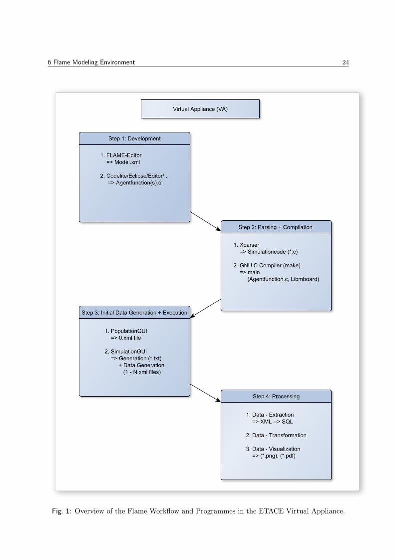
A Flame model development cycle goes through several stages, as illustrated in Fig.1.
6.1 What is FLAME?
In a nutshell:
- FLAME is a program generator. It generates a simulation executable from C and XML files.
- FLAME is a domain-specific language programmed in C, that provides facilities for higher-levelprogramming of economic and biological models.
- It uses the markup language XMML (X-Machine Modeling Language) for the declaration offunction and variables, and template files in C to generate the final C code of the model.
- All model functions are written in plain C code (a small subset of C), while the scheduling ofagents, functions and messages is coded in XML, with the help of an easy-to-use FLAMEEditor.
- The XML model file is then parsed by the Xparser, producing C code for the simulator. ThisC code is then compiled together with the user-provided C code for the agent functions,which generates the simulation executable.
- Libmboard (Message Board Library) provides facilities for message passing.
6.2 Flame Model Workflow
A detailed workflow can be found below. For producing new models quickly, we note that:
• To view a model and its agents, functions, messages, etc., use the FLAME Editor and openthe model.xml file.
• To generate initial data in an 0.xml file, use the Population GUI. Also use this to view oredit pre-existing .pop files (population description files). These files can be found in thesame /its folder as the default 0.xml file.
• In order to keep this image lightweight we do not provide a front-end for C programming.To view and edit the code, you can use vi, nano or leafpad, all available from the terminal.If required, additional programmes can be installed using the SliTaz package managertazpkg. For further detail on that, we refer here to the SliTaz documentation.
• Once you have created a new model.xml or 0.xml file, use the xparser to parse and compilethe model. After double- clicking the desktop shortcut, choose the model.xml file (usuallycalled eurace model.xml). After x-parsing the model you will be prompted to press ENTERto compile the model2.
2 For advanced users: the GUI version of the xparser does not provide any additional options. If you requirethese, you will have to run the xparser from the command line: /home/eurace/Desktop/Models/xparser-gsl/xparser.Options include: -p: parallel code, -f: final production mode.
6 Flame Modeling Environment 24
Fig. 1: Overview of the Flame Workflow and Programmes in the ETACE Virtual Appliance.
7 Licensing 25
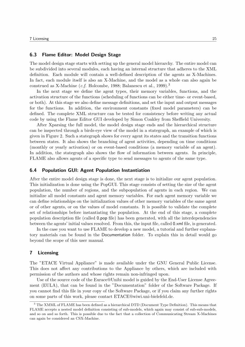
6.3 Flame Editor: Model Design Stage
The model design stage starts with setting up the general model hierarchy. The entire model canbe subdivided into several modules, each having an internal structure that adheres to the XMLdefinition. Each module will contain a well-defined description of the agents as X-Machines.In fact, each module itself is also an X-Machine, and the model as a whole can also again beconstrued as X-Machine (c.f. Holcombe, 1988; Balanescu et al., 1999).3
In the next stage we define the agent types, their memory variables, functions, and theactivation structure of the functions (scheduling of functions can be either time- or event-based,or both). At this stage we also define message definitions, and set the input and output messagesfor the functions. In addition, the environment constants (fixed model parameters) can bedefined. The complete XML structure can be tested for consistency before writing any actualcode by using the Flame Editor GUI developed by Simon Coakley from Sheffield University.
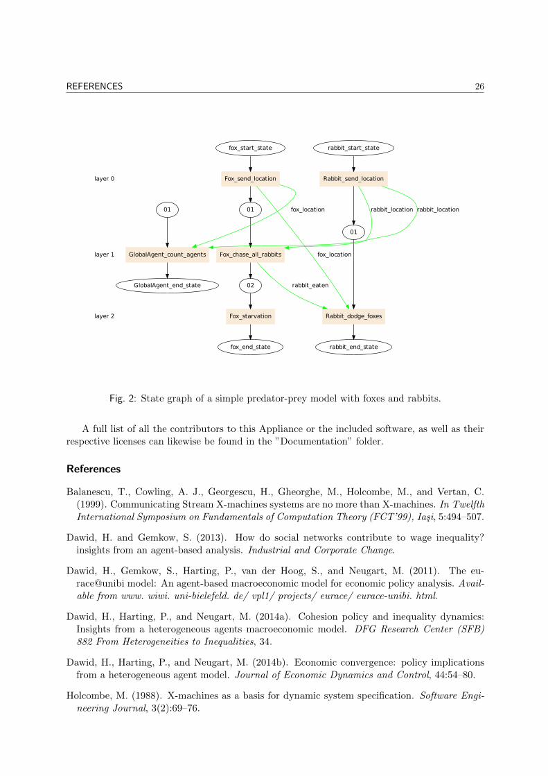
After Xparsing the full model, the model design stage ends and the hierarchical structurecan be inspected through a birds-eye view of the model in a stategraph, an example of which isgiven in Figure 2. Such a stategraph shows for every agent its states and the transition functionsbetween states. It also shows the branching of agent activities, depending on time conditions(monthly or yearly activation) or on event-based conditions (a memory variable of an agent).In addition, the stategraph also shows the flow of information between agents. In principle,FLAME also allows agents of a specific type to send messages to agents of the same type.
6.4 Population GUI: Agent Population Instantiation
After the entire model design stage is done, the next stage is to initialize our agent population.This initialization is done using the PopGUI. This stage consists of setting the size of the agentpopulation, the number of regions, and the subpopulation of agents in each region. We caninitialize all model constants and agent memory variables. For each agent memory variable wecan define relationships on the initialization values of other memory variables of the same agentor of other agents, or on the values of model constants. It is possible to validate the completeset of relationships before instantiating the population. At the end of this stage, a completepopulation description file (called 0.pop file) has been generated, with all the interdependenciesbetween the agents’ initial values resolved. From this, the input file, called 0.xml file, is generated.
In the case you want to use FLAME to develop a new model, a tutorial and further explana-tory materials can be found in the Documentation folder. To explain this in detail would gobeyond the scope of this user manual.
7 Licensing
The ”ETACE Virtual Appliance” is made available under the GNU General Public License.This does not affect any contributions to the Appliance by others, which are included withpermission of the authors and whose rights remain non-infringed upon.
Use of the source code of the Eurace@Unibi model is guided by the End-User License Agree-ment (EULA), that can be found in the ”Documentation” folder of the Software Package. Ifyou cannot find this file in your copy of the Software Package, or if you claim any further rightson some parts of this work, please contact [email protected].
3 The XMML of FLAME has been defined as a hierarchical DTD (Document Type Definition). This means thatFLAME accepts a nested model definition consisting of sub-models, which again may consist of sub-sub-models,and so on and so forth. This is possible due to the fact that a collection of Communicating Stream X-Machinescan again be considered an CSX-Machine.
REFERENCES 26
layer 0
layer 1
layer 2
fox_end_state
02
Fox_starvation
01
Fox_chase_all_rabbits
fox_start_state
Fox_send_location
rabbit_end_state
01
Rabbit_dodge_foxes
rabbit_start_state
Rabbit_send_location
GlobalAgent_end_state
01
GlobalAgent_count_agents fox_location
fox_location
rabbit_eaten
rabbit_location rabbit_location
Fig. 2: State graph of a simple predator-prey model with foxes and rabbits.
A full list of all the contributors to this Appliance or the included software, as well as theirrespective licenses can likewise be found in the ”Documentation” folder.
References
Balanescu, T., Cowling, A. J., Georgescu, H., Gheorghe, M., Holcombe, M., and Vertan, C.(1999). Communicating Stream X-machines systems are no more than X-machines. In TwelfthInternational Symposium on Fundamentals of Computation Theory (FCT’99), Iasi, 5:494–507.
Dawid, H. and Gemkow, S. (2013). How do social networks contribute to wage inequality?insights from an agent-based analysis. Industrial and Corporate Change.
Dawid, H., Gemkow, S., Harting, P., van der Hoog, S., and Neugart, M. (2011). The eu-race@unibi model: An agent-based macroeconomic model for economic policy analysis. Avail-able from www. wiwi. uni-bielefeld. de/ vpl1/ projects/ eurace/ eurace-unibi. html.
Dawid, H., Harting, P., and Neugart, M. (2014a). Cohesion policy and inequality dynamics:Insights from a heterogeneous agents macroeconomic model. DFG Research Center (SFB)882 From Heterogeneities to Inequalities, 34.
Dawid, H., Harting, P., and Neugart, M. (2014b). Economic convergence: policy implicationsfrom a heterogeneous agent model. Journal of Economic Dynamics and Control, 44:54–80.
Holcombe, M. (1988). X-machines as a basis for dynamic system specification. Software Engi-neering Journal, 3(2):69–76.

REFERENCES 27
Stodden, V. C. (2010). Reproducible research: Addressing the need for data and code sharingin computational science. Computing in Science & Engineering, 12(5):8–12.