Embed Size (px)
Citation preview

American Mineralogist, Volume 91, pages 635�657, 2006
0003-004X/06/0004�635$05.00/DOI: 10.2138/am.2006.1845 635
INTRODUCTION
Analysis of the chemical composition and bulk molar volume (or density) of ß uid inclusions in minerals has undergone major advances in recent years with the advent of new quantitative ana-lytical techniques, with the growth of the experimental database on the pressure, temperature, molar volume, and compositional (P-T-Vm-x) properties of geological ß uids, and with the devel-opment of theoretical methods to model these ß uids (for recent reviews see Andersen et al. 2001; Samson et al. 2003). Despite these advances, the analysis of saline aqueous inclusions that con-tain appreciable amounts of volatile components (e.g., CO2, CH4, H2S, and N2), which are common in diagenetic, hydrothermal, metamorphic, and igneous rocks, remains problematic. This is because the available equations-of-state for elevated P-T condi-tions are unable to link accurately high-T microthermometric measurements (homogenization temperatures) with low-tem-perature observations. The calculation of bulk properties still relies on notoriously inaccurate optical estimates of the volume
fractions of phases (e.g., liquid and vapor) within the inclusions. Uncertainty in the phase volume-fractions is usually the greatest single contributor to the overall uncertainty in bulk Vm � x proper-ties of this important class of ß uid inclusions (Diamond 2003a). Moreover, for most ß uid-inclusion shapes, the magnitude of the uncertainty in volume fractions is unknown.
In addition to their use in calculating bulk inclusion proper-ties, the volume fractions of phases in ß uid inclusions at room temperature are routinely estimated during fluid inclusion petrography to deduce whether assemblages of cogenetic inclu-sions were originally trapped from a one-phase or a multi-phase pore ß uid (e.g., Diamond 2003b). Although the absolute values of the volume fractions are less important for this purpose, and although other checks on the uniformity of compositions and densities can be made via microthermometry, the uncertainties currently inherent in determining the relative differences between cogenetic inclusions may lead to erroneous interpretations.
For ß uids that ß uoresce in ultraviolet light, such as petro-leum-bearing inclusions, Pironon et al. (1998) and Aplin et al. (1999) showed that phase volume-fractions can be determined with acceptable accuracy using scanning confocal ß uorescent * E-mail: [email protected]
Estimation of volume fractions of liquid and vapor phases in ß uid inclusions, and deÞ nition of inclusion shapes
RONALD J. BAKKER1,* AND LARRYN W. DIAMOND2
1Department of Applied Geosciences and Geophysics, Mineralogy and Petrology Group, University of Leoben, Peter-Tunner-Strasse 5, A-8700 Leoben, Austria
2Institute of Geological Sciences, University of Bern, Baltzerstrasse 1-3, CH-3012 Bern, Switzerland
ABSTRACT
The molar volume (Vm) and chemical composition (x) of saline aqueous inclusions and gas inclu-sions in minerals can be calculated satisfactorily from microthermometric and other analytical data. For complex gas-bearing aqueous inclusions, however, calculation of Vm � x properties requires additional input of the volume-fractions of the inclusion phases (φ). Traditional estimation of φ in non-ß uoresc-ing inclusions involves measuring area-fractions of the phases projected in the microscope and then making rough corrections for the third dimension. The uncertainties in the results are unknown and therefore the accuracies of the calculated Vm � x properties are also unknown.
To alleviate this problem we present a new, routine method to estimate φ using the petrographic microscope in conjunction with a spindle-stage. Inclusions in normal thick-sections are rotated stepwise and their projected areas and area-fractions are plotted against rotation angle. The resulting data arrays are systematically related to inclusion orientation, to inclusion shape, and to φ. The dependency on orientation is minimized when area fractions are measured at the position where the inclusions project their largest total areas. The shape dependency is accounted for using a new objective classiÞ cation of inclusion projections, based on parameters from digital image processing. The method has been veriÞ ed with synthetic ß uid inclusions of known φ. For individual liquid + vapor inclusions with regular (not �negative-crystal�) shapes, the new procedure yields φ with a relative accuracy of ±4%. This degree of accuracy permits Vm � x properties of gas-bearing, aqueous ß uid inclusions to be calculated with sufÞ cient certainty for many geochemical applications. Even better accuracy (e.g., down to ±0.6%) can be obtained by combining results from several inclusions in the same homogeneously trapped petrographic assemblage.
Keywords: ß uid inclusions, new technique, shape deÞ nition, spindle stage, ß uid phase, volume fractions

BAKKER AND DIAMOND: ESTIMATION OF VOLUME FRACTIONS636
microscopy in reß ected-light mode. The method involves inte-grating depth-series of two-dimensional images of individual in-clusions, each with a very small optical depth-of-Þ eld. However, for the huge class of inclusions that do not contain ß uorescent hydrocarbon molecules, the problem of measuring volume frac-tions remains unsolved. Phase contrasts in reß ected light are too weak for reliable scanning confocal microscopy, and so most workers attempt to estimate phase volume-fractions from the two-dimensional projection (i.e., from the phase area-fraction) that is obtained using a conventional petrographic microscope illuminated by transmitted white light. The conversion from area- to volume-fractions is commonly performed by compar-ing the microscope image with published reference diagrams that display example inclusions with various three-dimensional shapes (e.g., Shepherd et al. 1985). Often a clue to the thickness of the inclusions along the z-axis can be obtained by varying the depth of focus within the sample, but on the whole the method is highly subjective and the results are at best semi-quantitative. As the petrographic microscope is still the most convenient instrument for routine ß uid inclusion studies, any progress in improving the accuracy of phase-volume estimates using this instrument, or at least in quantifying the uncertainties of these estimates, is highly desirable.
In view of the above situation, we re-evaluate in this study the use of the petrographic microscope to estimate volume fractions of liquid and vapor in two-phase inclusions at room temperature. Our aims are (1) to quantify the probable uncertainties and (2) to suggest measurement procedures that could minimize the uncertainties. We begin by deÞ ning the mathematical equations that relate phase volume-fractions to bulk composition and molar volume (density), and, using these equations, we demonstrate how errors in volume fractions propagate into bulk Vm � x analyses. After reviewing previous work on estimating phase volume-fractions, we explore the variability of the functional relationship between area fractions and volume fractions by simulating ß uid inclusions with well-deÞ ned geometrical shapes. The corresponding relationships that can result in real inclusions are then illustrated using measurements on synthetic inclusions with known bulk Vm � x properties. Here we compare results obtained by rotating individual inclusions on a spindle-stage with results from assemblages of inclusions viewed in Þ xed orientations. The empirical relationships between area fractions and volumes fractions are found to be systematic and predictable, and this opens the way for a reliable analytical methodology. The generalization of the results requires a simple, objective classiÞ cation of the shapes of ß uid inclusions. We therefore propose a new classiÞ cation based on parameters measurable from series of two-dimensional images of individual inclusions obtained at different angles of rotation under the microscope. Finally, we organize our Þ ndings into a set of recommendations for determining the uncertainties of phase volume-fraction mea-surements during routine petrographic analysis.
Use of phase volume-fractions in calculating ß uid inclusion composition and molar volume
The Standard International (S.I.) symbol for volume fraction is used here, namely, one of the two lower-case Greek letters for phi or �f�, indicating �fraction� (Diamond 2003c). Older ß uid
inclusion literature uses a variety of symbols and deÞ nitions, e.g., F for �degree of Þ ll�, meaning the extent to which the inclusion is Þ lled by liquid (the �vapor� being approximated by a vacuum); Fα for �volume fraction� of the subscripted phase; or Rα for �volume ratio� of the subscripted phase.
The volume fraction (φ) of a phase α in a ß uid inclusion is deÞ ned as:
ϕα
α =Volume of phase
Volume of inclusion where 0 ≤ φα ≤ 1. (1)
Accordingly, φα has the dimensions of volume/volume and therefore it is unitless. Because phases in multi-phase ß uid inclusions increase or diminish in size as a function of tem-perature, it is necessary to specify the temperature at which a volume-fraction measurement is made. For example, φvap(20 °C) = 0.40 indicates that a vapor bubble occupies 40 vol% of the inclusion at 20 °C. In general, optical estimates of φα become even more complicated if more than two phases are present in an inclusion. Therefore, ß uid inclusions that contain more than two phases at room temperature are usually heated until only two phases become stable, and the estimate of φα is made at this temperature.
The phase volume-fraction may be used along with other data to calculate the bulk Vm � x properties of inclusions consisting of liquid and vapor. From Equation 1 it follows that:
φliq = 1 � φvap (2)
where φliq and φvap are the volume fractions of the liquid and vapor phases, respectively. Thus, the bulk molar volume, Vm (or bulk density, ρ) of the inclusion is given by:
1 1
V V Vm
vap
mvap
vap
mliq
= +ϕ ϕ�
(3a)
ρ = φvap ⋅ ρvap + (1 � φvap) ⋅ ρliq (3b)
where Vmvap and Vm
liq are the individual molar volumes of the vapor and liquid phases, respectively, and ρvap and ρliq are the individual densities of the vapor and liquid phases, respectively. Values for the molar volumes of the individual phases must be obtained from independent sources and these must be valid for the temperature and pressure at which φvap is measured.
With bulk Vm now available from Equation 3a, the amount-of-substance fraction (hereafter referred to as the �mole fraction�) of the vapor in the bulk inclusion, xvap, can be calculated from:
xV V
V Vvap
m mliq
mvap
mliq
=−( )−( ) . (4)
Finally, the concentration of each component i in the inclusion can be obtained from a mass-balance equation:
xi = xvapxivap + (1 � xvap) xi
liq (5)
where xivap is the mole fraction of component i in the vapor and
xiliq is the mole fraction of component i in the liquid. Values for
these two parameters may be obtained from microthermometric, Raman spectroscopic, or other analytical methods. Equation 5
BAKKER AND DIAMOND: ESTIMATION OF VOLUME FRACTIONS 637
is solved repeatedly for each component, i. Examples of such calculations are given by Bakker and Diamond (2000) and Diamond (2003a). The program package of Bakker (2003) in-corporates equations equivalent to Equations 3 to 5 above, and performs calculations based on input from microthermometry and Raman analysis.
The dependency of bulk properties on φvap can be illustrated by solving Equations 3 to 5 for a speciÞ c example. For a particularly simple, binary case, consider a CO2-H2O ß uid inclusion in which a liquid carbonic phase (car), a carbonic vapor, and an aqueous liquid (aq) are stable at low temperatures (e.g., 15 °C). This ex-ample corresponds to one of the synthetic ß uid inclusions that is analyzed in a following section. The carbonic phases homogenize to liquid at 18 °C. At this temperature the internal pressure in the inclusion is 5.47 MPa, and Vm
car = 55.44 cm3/mol and Vmaq =
18.39 cm3/mol (all values from the EoS of Diamond and AkinÞ ev 2003). If the measured volume fraction of the carbonic liquid is 54%, then solution of Equations 3 to 5 yields xCO2
= 30% and Vm = 28.87 cm3/mol. This example demonstrates that knowledge of the total homogenization temperature is not required to determine the bulk Vm � x properties if φvap can be measured.
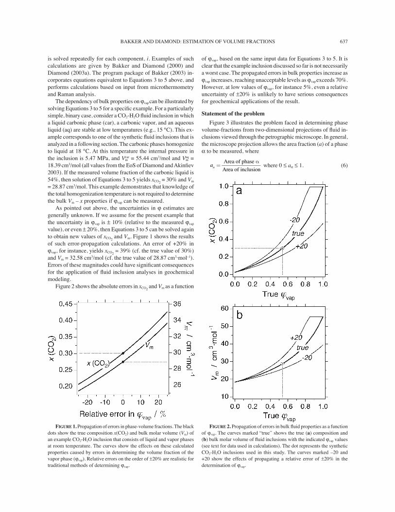
As pointed out above, the uncertainties in φ estimates are generally unknown. If we assume for the present example that the uncertainty in φvap is ± 10% (relative to the measured φvap
value), or even ± 20%, then Equations 3 to 5 can be solved again to obtain new values of xCO2
and Vm. Figure 1 shows the results of such error-propagation calculations. An error of +20% in φvap, for instance, yields xCO2
= 39% (cf. the true value of 30%) and Vm = 32.58 cm3/mol (cf. the true value of 28.87 cm3·mol�1). Errors of these magnitudes could have signiÞ cant consequences for the application of ß uid inclusion analyses in geochemical modeling.
Figure 2 shows the absolute errors in xCO2 and Vm as a function
of φvap, based on the same input data for Equations 3 to 5. It is clear that the example inclusion discussed so far is not necessarily a worst case. The propagated errors in bulk properties increase as φvap increases, reaching unacceptable levels as φvap exceeds 70%. However, at low values of φvap, for instance 5%, even a relative uncertainty of ±20% is unlikely to have serious consequences for geochemical applications of the result.
Statement of the problem
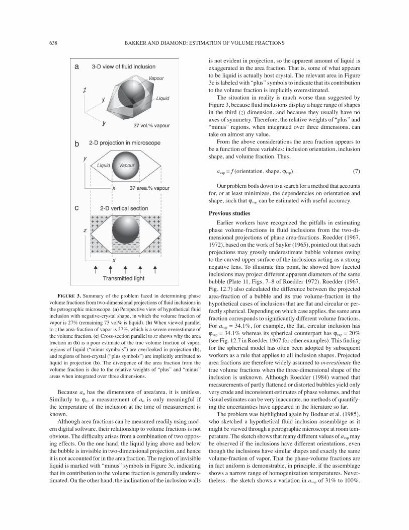
Figure 3 illustrates the problem faced in determining phase volume-fractions from two-dimensional projections of ß uid in-clusions viewed through the petrographic microscope. In general, the microscope projection allows the area fraction (a) of a phase α to be measured, where
aa =Area of phase
Area of inclusion
α where 0 ≤ aα ≤ 1. (6)
FIGURE 1. Propagation of errors in phase-volume fractions. The black dots show the true composition x(CO2) and bulk molar volume (Vm) of an example CO2-H2O inclusion that consists of liquid and vapor phases at room temperature. The curves show the effects on these calculated properties caused by errors in determining the volume fraction of the vapor phase (φvap). Relative errors on the order of ±20% are realistic for traditional methods of determining φvap.
FIGURE 2. Propagation of errors in bulk ß uid properties as a function of φvap. The curves marked �true� shows the true (a) composition and (b) bulk molar volume of ß uid inclusions with the indicated φvap values (see text for data used in calculations). The dot represents the synthetic CO2-H2O inclusions used in this study. The curves marked �20 and +20 show the effects of propagating a relative error of ±20% in the determination of φvap.
BAKKER AND DIAMOND: ESTIMATION OF VOLUME FRACTIONS638
Because aα has the dimensions of area/area, it is unitless. Similarly to φα, a measurement of aα is only meaningful if the temperature of the inclusion at the time of measurement is known.
Although area fractions can be measured readily using mod-ern digital software, their relationship to volume fractions is not obvious. The difÞ culty arises from a combination of two oppos-ing effects. On the one hand, the liquid lying above and below the bubble is invisible in two-dimensional projection, and hence it is not accounted for in the area fraction. The region of invisible liquid is marked with �minus� symbols in Figure 3c, indicating that its contribution to the volume fraction is generally underes-timated. On the other hand, the inclination of the inclusion walls
is not evident in projection, so the apparent amount of liquid is exaggerated in the area fraction. That is, some of what appears to be liquid is actually host crystal. The relevant area in Figure 3c is labeled with �plus� symbols to indicate that its contribution to the volume fraction is implicitly overestimated.
The situation in reality is much worse than suggested by Figure 3, because ß uid inclusions display a huge range of shapes in the third (z) dimension, and because they usually have no axes of symmetry. Therefore, the relative weights of �plus� and �minus� regions, when integrated over three dimensions, can take on almost any value.
From the above considerations the area fraction appears to be a function of three variables: inclusion orientation, inclusion shape, and volume fraction. Thus,
avap = f (orientation, shape, φvap). (7)
Our problem boils down to a search for a method that accounts for, or at least minimizes, the dependencies on orientation and shape, such that φvap can be estimated with useful accuracy.
Previous studies
Earlier workers have recognized the pitfalls in estimating phase volume-fractions in ß uid inclusions from the two-di-mensional projections of phase area-fractions. Roedder (1967, 1972), based on the work of Saylor (1965), pointed out that such projections may grossly underestimate bubble volumes owing to the curved upper surface of the inclusions acting as a strong negative lens. To illustrate this point, he showed how faceted inclusions may project different apparent diameters of the same bubble (Plate 11, Figs. 7�8 of Roedder 1972). Roedder (1967, Fig. 12.7) also calculated the difference between the projected area-fraction of a bubble and its true volume-fraction in the hypothetical cases of inclusions that are ß at and circular or per-fectly spherical. Depending on which case applies, the same area fraction corresponds to signiÞ cantly different volume fractions. For avap = 34.1%, for example, the ß at, circular inclusion has φvap = 34.1% whereas its spherical counterpart has φvap = 20% (see Fig. 12.7 in Roedder 1967 for other examples). This Þ nding for the spherical model has often been adopted by subsequent workers as a rule that applies to all inclusion shapes. Projected area fractions are therefore widely assumed to overestimate the true volume fractions when the three-dimensional shape of the inclusion is unknown. Although Roedder (1984) warned that measurements of partly ß attened or distorted bubbles yield only very crude and inconsistent estimates of phase volumes, and that visual estimates can be very inaccurate, no methods of quantify-ing the uncertainties have appeared in the literature so far.
The problem was highlighted again by Bodnar et al. (1985), who sketched a hypothetical ß uid inclusion assemblage as it might be viewed through a petrographic microscope at room tem-perature. The sketch shows that many different values of avap may be observed if the inclusions have different orientations, even though the inclusions have similar shapes and exactly the same volume-fraction of vapor. That the phase-volume fractions are in fact uniform is demonstrable, in principle, if the assemblage shows a narrow range of homogenization temperatures. Never-theless, the sketch shows a variation in avap of 31% to 100%,
FIGURE 3. Summary of the problem faced in determining phase volume fractions from two-dimensional projections of ß uid inclusions in the petrographic microscope. (a) Perspective view of hypothetical ß uid inclusion with negative-crystal shape, in which the volume fraction of vapor is 27% (remaining 73 vol% is liquid). (b) When viewed parallel to z the area-fraction of vapor is 37%, which is a severe overestimate of the volume fraction. (c) Cross-section parallel to xz shows why the area fraction in (b) is a poor estimate of the true volume fraction of vapor; regions of liquid (�minus symbols�) are overlooked in projection (b), and regions of host-crystal (�plus symbols�) are implicitly attributed to liquid in projection (b). The divergence of the area fraction from the volume fraction is due to the relative weights of �plus� and �minus� areas when integrated over three dimensions.

BAKKER AND DIAMOND: ESTIMATION OF VOLUME FRACTIONS 639
implying that optical estimates of the volume fractions would have an enormous uncertainty if no information were obtainable on the thickness and shape of the inclusions in the z-axis. One could easily infer from this diagram that optical estimates of phase volume-fractions are too unreliable to be useful.
In recognition of the need for information on the shapes and thicknesses of inclusions in the z-axis, Anderson and Bodnar (1993) developed a spindle stage, which allows inclusion-bearing samples to be rotated about a horizontal axis and simultaneously viewed through the petrographic microscope at moderate magni-Þ cation (e.g., using 40× or 36× long working-distance objective lenses). Although this stage has since been applied to character-ize single inclusions for sophisticated analytical techniques, its application to determining phase volume-fractions in routine petrography has been limited. For the normal case, in which thick sections that contain many inclusions need to be examined prior to performing microthermometry, the optical clarity obtain-able with the spindle stage usually restricts viewing to angles of rotation of less than 60°. This restriction is critical; it precludes the most obvious approach to solving the volume-fraction prob-lem, namely of viewing individual inclusions at 90° intervals of rotation and then integrating to obtain volumes. A proven methodology of how to conduct volume-fraction measurements under routine, sub-optimal conditions is lacking.
Geometrical modeling of volume fractions
In a Þ rst step towards quantifying the dependency of area fraction on inclusion orientation and shape (according to Eq. 7), we explore the behavior of simple symmetrical shapes as models of ß uid inclusions under the microscope. The aim of this exercise is to search for any promising systematic features or �rules of thumb� that may be exploited in a methodology for real asymmetrical inclusions.
The simplest case is when the inclusions are perfectly ß at. Such inclusions pose no problems for determining phase volume fractions from two-dimensional projections, because as inclusion thickness (z) approaches zero,
limz 0
vap vap→⎡⎣
⎤⎦ =a ϕ . (8)
This relationship holds true even if the inclusions are not oriented perpendicular to the optical axis of the microscope. The accuracy of the φvap estimate therefore depends only on the certainty to which �ß atness� can be recognized, and on the accuracy of the area measurements themselves.
Most inclusions have a Þ nite thickness, and indeed gas-bear-ing aqueous inclusions, which are our main interest in this study, tend to have shapes that are more equant than those of gas-free aqueous inclusions (gas-bearing ß uids wet mineral surfaces less readily). As demonstrated by Roedder (1967, 1972), spherical inclusions are also easy to deal with (see below), but they are rare in nature. Therefore, in addition to the spherical case we present numerical simulations of the relationships between avap and φvap
for four hypothetical, geometrical shapes. The Þ ve models have been chosen to illustrate how different these relationships can be; they are not intended to cover all possible shapes of natural ß uid inclusions.
Each model inclusion consists of a vapor bubble surrounded
by liquid. Conceptually, the vapor is considered to expand pro-gressively until it Þ lls the inclusion completely. At each step in the expansion the orthogonally projected area fraction of the bubble (avap) is calculated and plotted against the corresponding volume fraction of the bubble (φvap). No account is taken of pos-sible lens affects due to non-orthogonal refraction, as mentioned by Roedder (1972). In other words, the host crystal and the two ß uid phases within the inclusion are all assumed to have the same index of refraction.
A spherical ß uid inclusion has been modeled in Figure 4 so as to familiarize the reader with our choice of graphical display using a well-known example (cf. Roedder 1967). The vapor bubble is also assumed to be spherical, corresponding to minimal surface free-energy, therefore projections in any direction are equivalent; they all result in the same values of avap. The bubble is able to maintain its spherical form over all values of φvap, i.e., it is never deformed by the walls of the inclusion. In Figure 4 the curve labeled �s� lies entirely above the short-dashed 1:1 reference line, indicating that avap is always an overestimate of φvap (in a real inclusion the meniscus between vapor and liquid would probably become invisible at φvap > 90%, owing to internal refraction of the transmitted light at the inclusion walls). The maximum relative divergence between avap and φvap, deÞ ned as (avap � φvap )/φvap, occurs at a low value of φvap (< 10 vol%), whereas the maximum absolute divergence (avap � φvap = +14.8%) occurs at 30 vol%.
A cylindrical inclusion terminated by hemispheres (Fig. 4) reveals a different correlation between avap and φvap. In the pro-jection parallel to the long axis of this inclusion (a in Fig. 4), both the inclusion and the bubble have circular outlines. For the inclusion dimensions chosen for this example, the bubble is able to expand spherically up to 22.2 vol% without being constrained by the walls of the inclusion (zone 1 in Fig. 4). At 22.2 vol% the
FIGURE 4. Volume fraction vs. area fraction diagram of the vapor bubble in spherical and cylindrical ß uid inclusions. The cylinder has a relative length of 28 and a radius of 6. The ends of the cylinder are hemispheres with a radius of 6. The spherical inclusion projects equally in all directions (s), whereas the cylindrical inclusion appears spherical in the a projection and elongate in the b projection. See text for further details.
BAKKER AND DIAMOND: ESTIMATION OF VOLUME FRACTIONS640
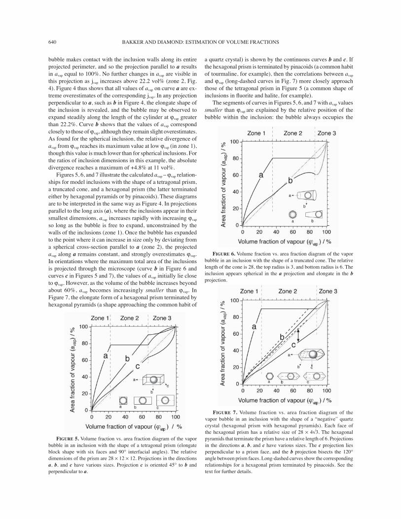
bubble makes contact with the inclusion walls along its entire projected perimeter, and so the projection parallel to a results in avap equal to 100%. No further changes in avap are visible in this projection as jvap increases above 22.2 vol% (zone 2, Fig. 4). Figure 4 thus shows that all values of avap on curve a are ex-treme overestimates of the corresponding jvap. In any projection perpendicular to a, such as b in Figure 4, the elongate shape of the inclusion is revealed, and the bubble may be observed to expand steadily along the length of the cylinder at φvap greater than 22.2%. Curve b shows that the values of avap correspond closely to those of φvap, although they remain slight overestimates. As found for the spherical inclusion, the relative divergence of avap from φvap reaches its maximum value at low φvap (in zone 1), though this value is much lower than for spherical inclusions. For the ratios of inclusion dimensions in this example, the absolute divergence reaches a maximum of +4.8% at 11 vol%.
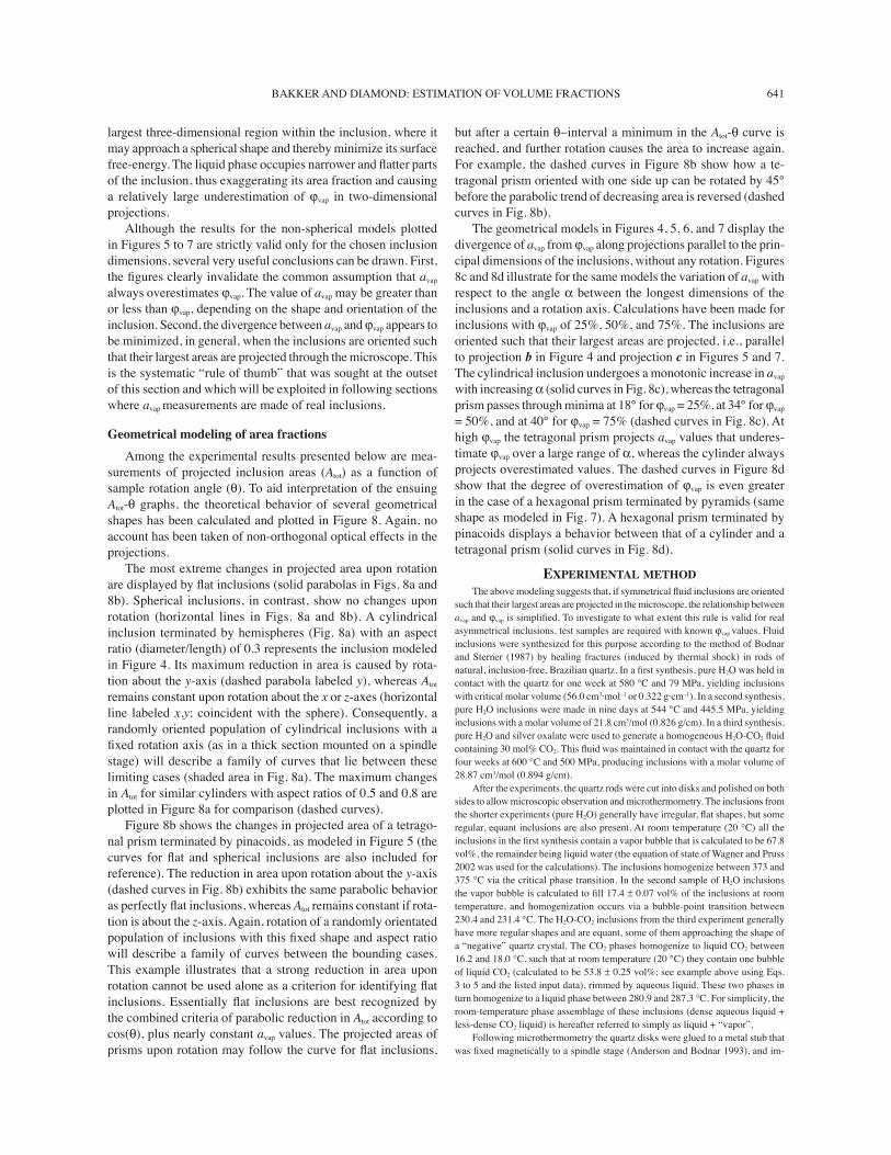
Figures 5, 6, and 7 illustrate the calculated avap � φvap relation-ships for model inclusions with the shape of a tetragonal prism, a truncated cone, and a hexagonal prism (the latter terminated either by hexagonal pyramids or by pinacoids). These diagrams are to be interpreted in the same way as Figure 4. In projections parallel to the long axis (a), where the inclusions appear in their smallest dimensions, avap increases rapidly with increasing φvap so long as the bubble is free to expand, unconstrained by the walls of the inclusions (zone 1). Once the bubble has expanded to the point where it can increase in size only by deviating from a spherical cross-section parallel to a (zone 2), the projected avap along a remains constant, and strongly overestimates φvap. In orientations where the maximum total area of the inclusions is projected through the microscope (curve b in Figure 6 and curves c in Figures 5 and 7), the values of avap initially lie close to φvap. However, as the volume of the bubble increases beyond about 60%, avap becomes increasingly smaller than φvap. In Figure 7, the elongate form of a hexagonal prism terminated by hexagonal pyramids (a shape approaching the common habit of
a quartz crystal) is shown by the continuous curves b and c. If the hexagonal prism is terminated by pinacoids (a common habit of tourmaline, for example), then the correlations between avap and φvap (long-dashed curves in Fig. 7) more closely approach those of the tetragonal prism in Figure 5 (a common shape of inclusions in ß uorite and halite, for example).
The segments of curves in Figures 5, 6, and 7 with avap values smaller than φvap are explained by the relative position of the bubble within the inclusion: the bubble always occupies the
FIGURE 5. Volume fraction vs. area fraction diagram of the vapor bubble in an inclusion with the shape of a tetragonal prism (elongate block shape with six faces and 90° interfacial angles). The relative dimensions of the prism are 28 × 12 × 12. Projections in the directions a, b, and c have various sizes. Projection c is oriented 45° to b and perpendicular to a.
FIGURE 6. Volume fraction vs. area fraction diagram of the vapor bubble in an inclusion with the shape of a truncated cone. The relative length of the cone is 28, the top radius is 3, and bottom radius is 6. The inclusion appears spherical in the a projection and elongate in the b projection.
FIGURE 7. Volume fraction vs. area fraction diagram of the vapor bubble in an inclusion with the shape of a �negative� quartz crystal (hexagonal prism with hexagonal pyramids). Each face of the hexagonal prism has a relative size of 28 × 4√3. The hexagonal pyramids that terminate the prism have a relative length of 6. Projections in the directions a, b, and c have various sizes. The c projection lies perpendicular to a prism face, and the b projection bisects the 120° angle between prism faces. Long-dashed curves show the corresponding relationships for a hexagonal prism terminated by pinacoids. See the text for further details.
BAKKER AND DIAMOND: ESTIMATION OF VOLUME FRACTIONS 641
largest three-dimensional region within the inclusion, where it may approach a spherical shape and thereby minimize its surface free-energy. The liquid phase occupies narrower and ß atter parts of the inclusion, thus exaggerating its area fraction and causing a relatively large underestimation of φvap in two-dimensional projections.
Although the results for the non-spherical models plotted in Figures 5 to 7 are strictly valid only for the chosen inclusion dimensions, several very useful conclusions can be drawn. First, the Þ gures clearly invalidate the common assumption that avap always overestimates φvap. The value of avap may be greater than or less than φvap, depending on the shape and orientation of the inclusion. Second, the divergence between avap and φvap appears to be minimized, in general, when the inclusions are oriented such that their largest areas are projected through the microscope. This is the systematic �rule of thumb� that was sought at the outset of this section and which will be exploited in following sections where avap measurements are made of real inclusions.
Geometrical modeling of area fractions
Among the experimental results presented below are mea-surements of projected inclusion areas (Atot) as a function of sample rotation angle (θ). To aid interpretation of the ensuing Atot-θ graphs, the theoretical behavior of several geometrical shapes has been calculated and plotted in Figure 8. Again, no account has been taken of non-orthogonal optical effects in the projections.
The most extreme changes in projected area upon rotation are displayed by ß at inclusions (solid parabolas in Figs. 8a and 8b). Spherical inclusions, in contrast, show no changes upon rotation (horizontal lines in Figs. 8a and 8b). A cylindrical inclusion terminated by hemispheres (Fig. 8a) with an aspect ratio (diameter/length) of 0.3 represents the inclusion modeled in Figure 4. Its maximum reduction in area is caused by rota-tion about the y-axis (dashed parabola labeled y), whereas Atot remains constant upon rotation about the x or z-axes (horizontal line labeled x,y; coincident with the sphere). Consequently, a randomly oriented population of cylindrical inclusions with a Þ xed rotation axis (as in a thick section mounted on a spindle stage) will describe a family of curves that lie between these limiting cases (shaded area in Fig. 8a). The maximum changes in Atot for similar cylinders with aspect ratios of 0.5 and 0.8 are plotted in Figure 8a for comparison (dashed curves).
Figure 8b shows the changes in projected area of a tetrago-nal prism terminated by pinacoids, as modeled in Figure 5 (the curves for ß at and spherical inclusions are also included for reference). The reduction in area upon rotation about the y-axis (dashed curves in Fig. 8b) exhibits the same parabolic behavior as perfectly ß at inclusions, whereas Atot remains constant if rota-tion is about the z-axis. Again, rotation of a randomly orientated population of inclusions with this Þ xed shape and aspect ratio will describe a family of curves between the bounding cases. This example illustrates that a strong reduction in area upon rotation cannot be used alone as a criterion for identifying ß at inclusions. Essentially ß at inclusions are best recognized by the combined criteria of parabolic reduction in Atot according to cos(θ), plus nearly constant avap values. The projected areas of prisms upon rotation may follow the curve for ß at inclusions,
but after a certain θ−interval a minimum in the Atot-θ curve is reached, and further rotation causes the area to increase again. For example, the dashed curves in Figure 8b show how a te-tragonal prism oriented with one side up can be rotated by 45° before the parabolic trend of decreasing area is reversed (dashed curves in Fig. 8b).
The geometrical models in Figures 4, 5, 6, and 7 display the divergence of avap from φvap along projections parallel to the prin-cipal dimensions of the inclusions, without any rotation. Figures 8c and 8d illustrate for the same models the variation of avap with respect to the angle α between the longest dimensions of the inclusions and a rotation axis. Calculations have been made for inclusions with φvap of 25%, 50%, and 75%. The inclusions are oriented such that their largest areas are projected, i.e., parallel to projection b in Figure 4 and projection c in Figures 5 and 7. The cylindrical inclusion undergoes a monotonic increase in avap with increasing α (solid curves in Fig. 8c), whereas the tetragonal prism passes through minima at 18° for φvap = 25%, at 34° for φvap = 50%, and at 40° for φvap = 75% (dashed curves in Fig. 8c). At high φvap the tetragonal prism projects avap values that underes-timate φvap over a large range of α, whereas the cylinder always projects overestimated values. The dashed curves in Figure 8d show that the degree of overestimation of φvap is even greater in the case of a hexagonal prism terminated by pyramids (same shape as modeled in Fig. 7). A hexagonal prism terminated by pinacoids displays a behavior between that of a cylinder and a tetragonal prism (solid curves in Fig. 8d).
EXPERIMENTAL METHODThe above modeling suggests that, if symmetrical ß uid inclusions are oriented
such that their largest areas are projected in the microscope, the relationship between avap and φvap is simpliÞ ed. To investigate to what extent this rule is valid for real asymmetrical inclusions, test samples are required with known φvap values. Fluid inclusions were synthesized for this purpose according to the method of Bodnar and Sterner (1987) by healing fractures (induced by thermal shock) in rods of natural, inclusion-free, Brazilian quartz. In a Þ rst synthesis, pure H2O was held in contact with the quartz for one week at 580 °C and 79 MPa, yielding inclusions with critical molar volume (56.0 cm3·mol�1 or 0.322 g·cm�1). In a second synthesis, pure H2O inclusions were made in nine days at 544 °C and 445.5 MPa, yielding inclusions with a molar volume of 21.8 cm3/mol (0.826 g/cm). In a third synthesis, pure H2O and silver oxalate were used to generate a homogeneous H2O-CO2 ß uid containing 30 mol% CO2. This ß uid was maintained in contact with the quartz for four weeks at 600 °C and 500 MPa, producing inclusions with a molar volume of 28.87 cm3/mol (0.894 g/cm).
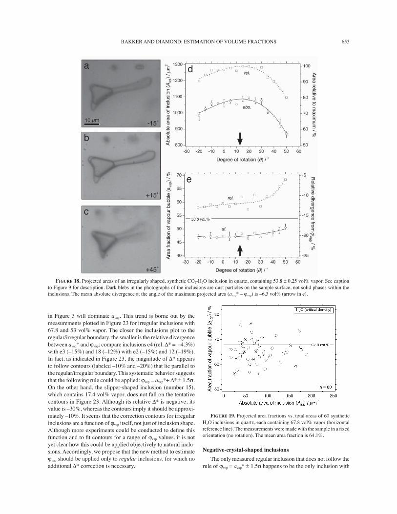
After the experiments, the quartz rods were cut into disks and polished on both sides to allow microscopic observation and microthermometry. The inclusions from the shorter experiments (pure H2O) generally have irregular, ß at shapes, but some regular, equant inclusions are also present. At room temperature (20 °C) all the inclusions in the Þ rst synthesis contain a vapor bubble that is calculated to be 67.8 vol%, the remainder being liquid water (the equation of state of Wagner and Pruss 2002 was used for the calculations). The inclusions homogenize between 373 and 375 °C via the critical phase transition. In the second sample of H2O inclusions the vapor bubble is calculated to Þ ll 17.4 ± 0.07 vol% of the inclusions at room temperature, and homogenization occurs via a bubble-point transition between 230.4 and 231.4 °C. The H2O-CO2 inclusions from the third experiment generally have more regular shapes and are equant, some of them approaching the shape of a �negative� quartz crystal. The CO2 phases homogenize to liquid CO2 between 16.2 and 18.0 °C, such that at room temperature (20 °C) they contain one bubble of liquid CO2 (calculated to be 53.8 ± 0.25 vol%; see example above using Eqs. 3 to 5 and the listed input data), rimmed by aqueous liquid. These two phases in turn homogenize to a liquid phase between 280.9 and 287.3 °C. For simplicity, the room-temperature phase assemblage of these inclusions (dense aqueous liquid + less-dense CO2 liquid) is hereafter referred to simply as liquid + �vapor�.
Following microthermometry the quartz disks were glued to a metal stub that was Þ xed magnetically to a spindle stage (Anderson and Bodnar 1993), and im-

BAKKER AND DIAMOND: ESTIMATION OF VOLUME FRACTIONS642
mersed in a cell containing oil with a refractive index similar to those of quartz. The assembly was mounted on a microscope with a 40× long-working-distance objective lens Þ tted with an adjustable cover-slip correction cap. The face of the objective lens was situated in air, above the upper level of immersion oil in the sample cell. The samples were viewed with a sub-stage condenser lens inserted into the light path. In this conÞ guration the convergent transmitted light entered the immersion oil from below the sample. The light then traversed the inclusion-bearing quartz sample, passed through the overlying oil, and exited into air before entering the objective lens. The spindle stage was thus used in the exactly the same way as described by Anderson and Bodnar (1993).
Each inclusion selected for area measurement was aligned approximately along the rotation axis of the spindle stage. The sample was then rotated in intervals of 5° and the inclusion was photographed digitally in each position. The value of avap in each microphotograph was measured by tracing digitally around the outside edges of the shadows that deÞ ne the perimeters of the bubble and the inclusion. Tests showed that tracing around the outside edges yielded the greatest reproducibility in avap, especially when different workers measured the same inclusion. Presumably the outermost outline best represents the true projection of the three-dimensional inclusion. Areas were integrated with the NIH image software package (version 1.63) or its successor, ImageJ (http://rsb.info.nih.gov/).
Owing to optical effects related to depth-of-focus and refraction, the clarity of the outlines of the inclusions and their bubbles varied with orientation of the disk. To help account for this inherent uncertainty, the avap measurements were repeated three times for each microphotograph. The Þ rst trace was performed in a clockwise direction, the second anticlockwise, and then the photograph was enlarged by 200% and traced a third time. In addition, the total area and the perimeter of each inclusion were measured from each microphotograph.
Several target inclusions had such irregular shapes that their entire outlines could not be brought into focus at any one vertical position of the microscope stage. Photographs were unsuitable in these cases, therefore the inclusion and bubble outlines were traced by hand using a projection tube mounted above the
trinocular head of the microscope. The scale drawings were then digitized and thereafter treated in the same way as the photographs.
RESULTS
Within each of the three synthetic ß uid inclusion samples, several inclusions representing a variety of shapes were selected for analysis. The aim was to search for reproducible patterns in the relationships of projection angle, ß uid inclusion area, and avap, with respect to φvap. The results for three representative inclusions from each sample are presented in the following. Additional re-sults are available on the authors� websites (http://ß uids.unileoben.ac.at/ and www.geo.unibe.ch/diamond). As a complement to the analyses of individual ß uid inclusions, measurements of avap were also made on assemblages of inclusions in each sample, with the quartz disks in Þ xed orientations. All measurements, on both individual inclusions and assemblages, were made at 20 °C.
Measurements of individual synthetic H2O inclusions with 67.8 vol% vapor
Figure 9 summarizes measurements on a slightly conical inclusion. Figures 9a�c show the view through the microscope at three angles of rotation (θ), with the axis of the spindle stage oriented parallel to the short dimension of the printed page. Thus, the long axis of the inclusion lies at about 70° from the axis of the spindle-stage (this is the angle α plotted in Figs. 8c and 8d). A θ value of zero is assigned to the horizontal position of the ß uid
FIGURE 8. Calculated projections of the geometrical inclusions in Figures 4 to 7. The arrow marked p shows the projection direction. (a) Projected total areas of flat, spherical, and cylindrical inclusions vs. angle of rotation θ (e.g., on a spindle stage) along axes x, y, and z. (b) Projected total areas of a tetragonal prism vs. angle of rotation, θ, along axes x, y, and z. (c) Projected area fractions of the vapor bubble in cylindrical (solid curves) and tetragonal-prism (dashed) inclusions, vs. the angle α between the longest dimension of the inclusion and a spindle-stage rotation axis. (d) Same as (c) but calculated for inclusions shaped like �negative� quartz crystals: hexagonal prisms terminated by pinacoids (solid curves) or by hexagonal pyramids (dashed).

BAKKER AND DIAMOND: ESTIMATION OF VOLUME FRACTIONS 643
inclusion sample in the spindle stage, a positive sign indicates rotation in a clockwise direction, and a minus sign denotes an anticlockwise rotation; for example, Figure 9a shows the inclu-sion after 55° anticlockwise rotation, whereas Figure 9c shows the same inclusion after 5° clockwise rotation.
Figures 9a�c are not perfectly sharp. Certain segments of the outlines in Figures 9a and 9c are fuzzy, and an optical artifact (a Becke line) is visible as a bright rim along the left side of the inclusion in Figure 9a and as a dark shadow in Figure 9b. The quality of the images is evidently less than optimal for area measurements, but it is typical of all the inclusions studied here, and it is typical of most ß uid inclusions in natural samples.
Figure 9d displays the projected area of the inclusion, Atot, as a function of rotation angle. The ranges of the triplicate measure-ments (in absolute values of μm2; see scale on left-hand ordinate) are indicated by the error bars, and the mean of each triplicate
is plotted as a circle. Because the quality of the images varies from one rotation position to another, the length of the error bars also varies in a unpredictable way. The entire set of data was regressed to a best-Þ t polynomial function to smooth the trends (solid curve, labeled �abs.�). It is obvious that the inclusion ap-pears smallest near 10° and that the projected area increases as the inclusion is rotated to �55°. The maximum projected area according to the Þ tted curve lies around �52° (marked by an arrow in Fig. 9d).
The mean values of the absolute areas plotted in Figure 9d have been recalculated relative to the maximum datum found at �55°. The square symbols in Figure 9d show these recalculated values (see scale on right-hand ordinate), and the dashed curve labeled �rel.� represents a best-Þ t polynomial function to the mean of each set of triplicate data. Thus, the largest mean area plots at 100% and the smallest area (found at 10° rotation) plots
FIGURE 9. Projected areas of a slightly conical, synthetic H2O inclusion in quartz, containing 67.8 vol% vapor. (a, b, c) Microscope projections of the inclusion at three different angles of rotation (θ) in the spindle stage (numbers indicate angles). The axis of rotation is schematically illustrated. (d) Absolute projected area of the inclusion (left-hand ordinate scale) and area relative to the maximum area (right-hand scale), both vs. θ. The arrow marks the angle at which the maximum area of the inclusion is projected. (e) Area fractions of the vapor bubble as a function of θ. The horizontal reference line indicates the volume fraction of vapor (67.8%). The solid curve shows the absolute values of the area fraction (with respect to the left-hand ordinate scale). The dashed curve (with respect to the right-hand scale) shows the relative divergence of the area fraction from the known volume fraction [(avap � φvap)/φvap]. The mean absolute divergence at the angle of the maximum projected area (avap* � φvap) is �1.5 vol% (arrow).
BAKKER AND DIAMOND: ESTIMATION OF VOLUME FRACTIONS644
at 54%. By comparison with Figure 8a, the form of the dashed Atot-θ curve conÞ rms that the inclusion is neither spherical (the line would be horizontal) nor perfectly ß at (the curve would drop to around 71% at 45° from the maximum, whereas the curve in Fig. 9d drops to only 76%). Also, the dashed curve undergoes no inß ections upon 45° of rotation, as would be the case if the inclusion had a tetragonal shape (cf. Fig. 8b).
Figure 9e displays avap as a function of rotation angle. The ranges of triplicate measurements are shown by the error bars and the mean values are indicated by circles, all with respect to the scale on the left-hand ordinate. The solid curve labeled �af.� shows the best-Þ t polynomial function. To illustrate the relationship between avap and φvap, the value of φvap (67.8%) is marked by the thick horizontal line, with respect to the same ordinate scale as avap. It is obvious that avap grossly overestimates φvap at θ values near 10°, but after more than �35° rotation the mean values of avap drop slightly below φvap. This behavior is reminiscent of the symmetrical cone plotted in Figure 6. For an inclusion with φvap equal to 67.8%, avap along the a projection (compare inset diagram a in Fig. 6 with Fig. 9c) lies well above the true φvap value, whereas along the b projection the value of avap underestimates φvap (compare inset diagram b in Fig. 6 with Fig. 9a). However, it is obvious that the inclusion in Figures 9a,b,c is not a perfectly symmetrical cone and that the rotation axis of the photographed inclusion is probably oriented between the a and b axes in Figure 6. The similarities between Figures 6 and 9 are therefore only qualitative.
The object of plotting the analyses in Figure 9 is to reveal any systematic relationships between avap and φvap. Although the avap-θ curve in Figure 9e intersects the φvap reference line at ap-proximately �35°, this fortunate angle cannot be deduced solely from the curves in Figure 9d; they show no special features at this angle. The only features of the curves that can be identiÞ ed objectively are the maxima. Figure 9e shows that, at the angle of these maxima (marked by the arrow at �52°), avap is still equal to φvap within the reproducibility of the measurements.
The mean relative divergence of avap from φvap is indicated in Figure 9e by the square symbols and by the dashed curve (both with respect to the scale on the right-hand ordinate). Thus, the mean avap at 10° rotation is seen to overestimate φvap by 18%, whereas at �52° rotation (arrow in Figure 9e), the mean avap underestimates φvap by only 2%.
Several of the regular-shaped inclusions analyzed below show a close match between avap and φvap at the rotation angle at which the maximum area of the inclusions is projected. For further reference this special angle is denoted by the symbol θ* and the corresponding value of avap by the symbol avap*. The position of θ* in each of the following Atot-θ and avap-θ diagrams is marked with heavy arrows.
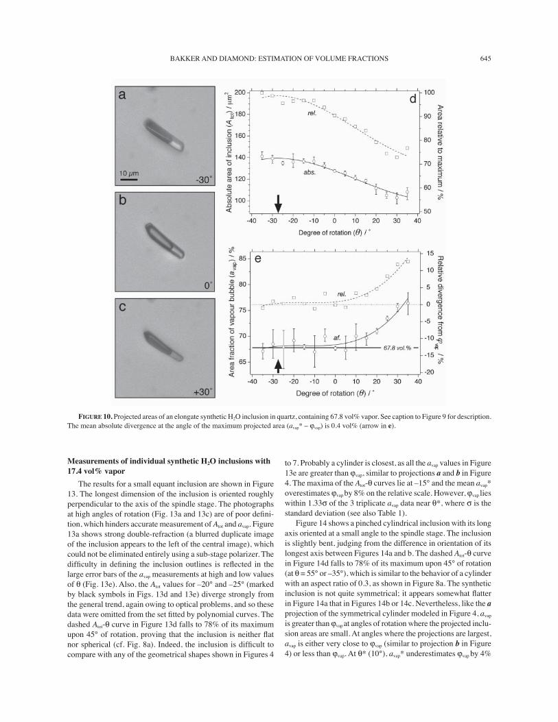
Figure 10 illustrates an elongate inclusion with a roughly cylindrical shape. The long axis of the inclusion is oriented at about 40° to the axis of the spindle stage. The cylindrical nature of the inclusion is demonstrated by its similar appearance over 60° of rotation (compare Fig. 10a at �30° with Fig. 10b at 0° and Fig. 10c at 30°). The Atot-θ curves in Figure 10d show maxima at �27° rotation. The dashed curve in Figure 10d, showing the area of the inclusion relative to its maximum area, is somewhat
similar to the dashed curve in Figure 8a, which represents a symmetrical cylinder with aspect ratio of 0.4; both curves fall to about 80% upon 45° rotation from θ*. As shown in Figure 10e, the measurements of avap for this inclusion are not very reproduc-ible (e.g., at �25° the range is from 64% to 71%). However, the regressed polynomial function (solid curve) provides a smooth trend. At +35°, where the inclusion displays its smallest area (cf. Fig. 10d), the value of avap strongly overestimates φvap (by 14% on the relative scale). This is not unlike the behavior of the symmetrical cylinder shown in Figure 4 (curve a) and Figure 8c (dashed curve 50 vol%), even though the axes of rotation are not quite comparable. Between 5° and �35° the avap-θ curve in Figure 10e ß attens out and lies very close to φvap, again similar to the behavior of a symmetrical cylinder (cf. curve b in Fig. 4). At θ*
(�27°), avap* matches φvap to well within the uncertainty
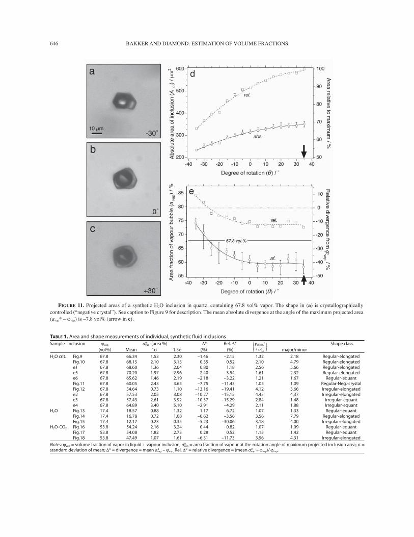
of the measurements. Figure 11 shows measurements for an approximately
equant inclusion with a distinct �negative-crystal� shape (most obvious in Figure 11a). The longest axis of the inclusion is oriented parallel to the axis of rotation of the spindle-stage. As in Figures 9 and 10, avap overestimates φvap at the rotation angle corresponding to the smallest observed projection of the inclusion (�35°). This is expected from qualitative comparison with the geometrical model in Figure 7 (projection b), even though the minimum area of the inclusion was not found in the analyses (the Atot-θ curves in Fig. 11d do not exhibit minima). Near the maxima in the Atot-θ curves (θ* = 35°), the values of avap level off at about 60%, strongly underestimating φvap (�12% divergence on the relative scale of Fig. 11e). Thus, in contrast to the regular-shaped inclusions in Figures 9 and 10, avap* is a very poor estimate of φvap.
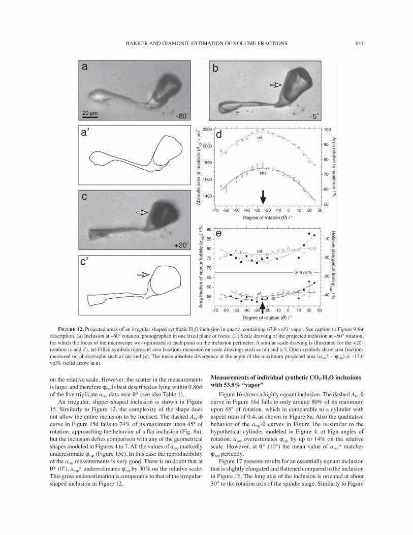
A large, highly irregular, ladle-shaped inclusion is displayed in Figure 12. The complexity of the shape in three dimensions made it impossible to focus the entire inclusion in the micro-scope at one time (cf. Figs. 12a, 12c). To provide more accurate outlines, drawings were made of the inclusion (see Experimental Method) by varying the focus level of the microscope (e.g., Fig. 12a' and 12c'). The open symbols in Figures 12d and e show triplicate measurements made from the set of partly focused photographs. The solid symbols in Figure 12e show avap mea-surements made on the drawings (one per 5° rotation interval). Between �55° and +10° rotation the results from the drawings are lower than those from the photographs, but the trend reverses at higher θ. The avap values from the drawings are probably more accurate. Their reproducibility compared to the photographic method cannot be assessed, because only one drawing was made per rotation interval. At θ* (�27°), as over much of the measured θ range, avap* underestimates φvap by 22% on the relative scale (dashed curve labeled �m� in Figure 12e). Evidently, the amount of liquid in the handle of the ladle is strongly exaggerated in the projections, similarly to the regions marked with plus symbols in Figure 3. The open arrows in the photographs in Figures 12b and c point to a rim of liquid between the vapor bubble and the inclusion wall. The drawings (Fig.12c�), however, show that this �rim� is an optical artifact (caused by non-orthogonal refraction of the transmitted light), and that the bubble actually extends to the inclusion wall.
BAKKER AND DIAMOND: ESTIMATION OF VOLUME FRACTIONS 645
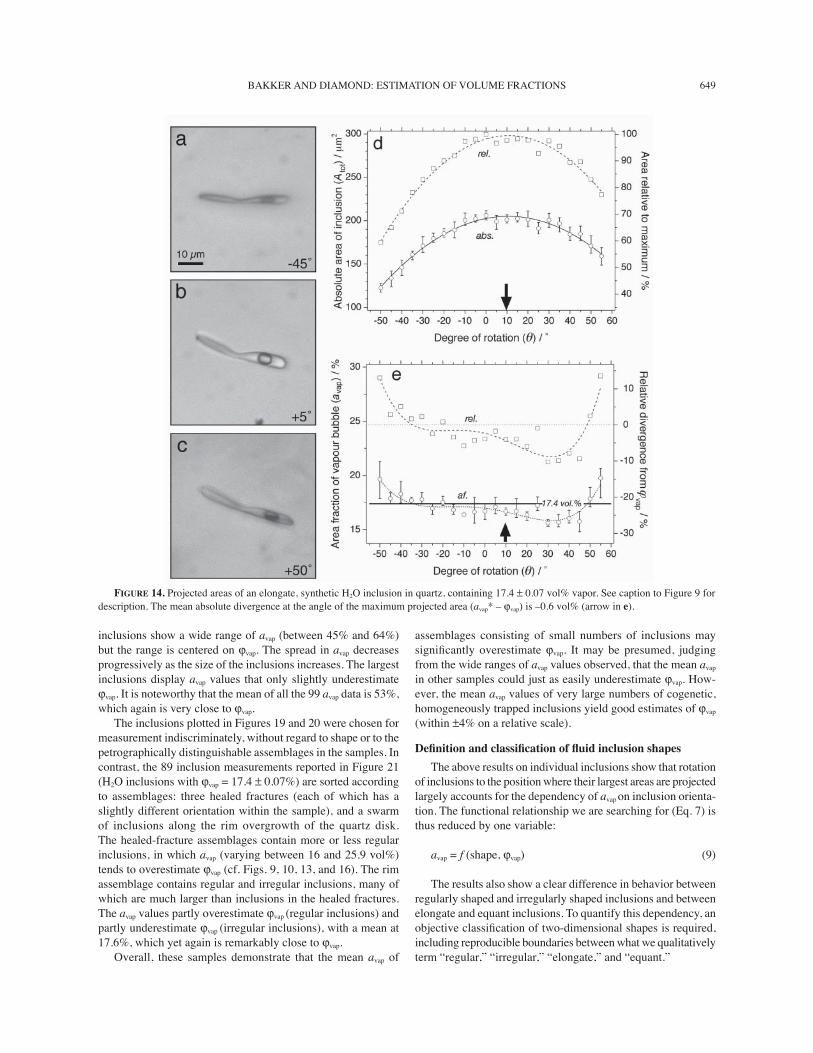
Measurements of individual synthetic H2O inclusions with 17.4 vol% vapor
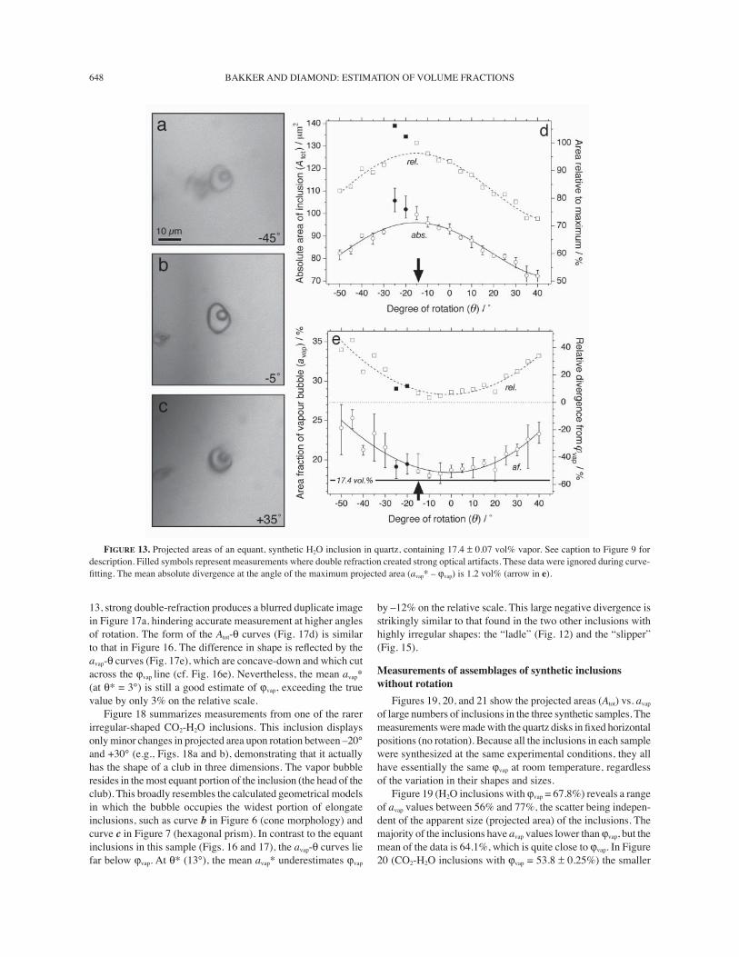
The results for a small equant inclusion are shown in Figure 13. The longest dimension of the inclusion is oriented roughly perpendicular to the axis of the spindle stage. The photographs at high angles of rotation (Fig. 13a and 13c) are of poor deÞ ni-tion, which hinders accurate measurement of Atot and avap. Figure 13a shows strong double-refraction (a blurred duplicate image of the inclusion appears to the left of the central image), which could not be eliminated entirely using a sub-stage polarizer. The difÞ culty in deÞ ning the inclusion outlines is reß ected in the large error bars of the avap measurements at high and low values of θ (Fig. 13e). Also, the Atot values for �20° and �25° (marked by black symbols in Figs. 13d and 13e) diverge strongly from the general trend, again owing to optical problems, and so these data were omitted from the set Þ tted by polynomial curves. The dashed Atot-θ curve in Figure 13d falls to 78% of its maximum upon 45° of rotation, proving that the inclusion is neither ß at nor spherical (cf. Fig. 8a). Indeed, the inclusion is difÞ cult to compare with any of the geometrical shapes shown in Figures 4
to 7. Probably a cylinder is closest, as all the avap values in Figure 13e are greater than φvap, similar to projections a and b in Figure 4. The maxima of the Atot-θ curves lie at �15° and the mean avap* overestimates φvap by 8% on the relative scale. However, φvap lies within 1.33σ of the 3 triplicate avap data near θ*, where σ is the standard deviation (see also Table 1).
Figure 14 shows a pinched cylindrical inclusion with its long axis oriented at a small angle to the spindle stage. The inclusion is slightly bent, judging from the difference in orientation of its longest axis between Figures 14a and b. The dashed Atot-θ curve in Figure 14d falls to 78% of its maximum upon 45° of rotation (at θ = 55° or �35°), which is similar to the behavior of a cylinder with an aspect ratio of 0.3, as shown in Figure 8a. The synthetic inclusion is not quite symmetrical; it appears somewhat ß atter in Figure 14a that in Figures 14b or 14c. Nevertheless, like the a projection of the symmetrical cylinder modeled in Figure 4, avap is greater than φvap at angles of rotation where the projected inclu-sion areas are small. At angles where the projections are largest, avap is either very close to φvap (similar to projection b in Figure 4) or less than φvap. At θ* (10°), avap* underestimates φvap by 4%
FIGURE 10. Projected areas of an elongate synthetic H2O inclusion in quartz, containing 67.8 vol% vapor. See caption to Figure 9 for description. The mean absolute divergence at the angle of the maximum projected area (avap* � φvap) is 0.4 vol% (arrow in e).
BAKKER AND DIAMOND: ESTIMATION OF VOLUME FRACTIONS646
FIGURE 11. Projected areas of a synthetic H2O inclusion in quartz, containing 67.8 vol% vapor. The shape in (a) is crystallographically controlled (�negative crystal�). See caption to Figure 9 for description. The mean absolute divergence at the angle of the maximum projected area (avap* � φvap) is �7.8 vol% (arrow in e).
TABLE 1. Area and shape measurements of individual, synthetic fl uid inclusionsSample Inclusion φvap a*vap (area %) Δ* Rel. Δ* Shape class (vol%) Mean 1σ 1.5σ (%) (%)
Perim.
4
2
totπA
⎛
⎝⎜⎜⎜⎜
⎞
⎠⎟⎟⎟⎟⎟ major/minor
H2O crit. Fig.9 67.8 66.34 1.53 2.30 –1.46 –2.15 1.32 2.18 Regular-elongated Fig.10 67.8 68.15 2.10 3.15 0.35 0.52 2.10 4.79 Regular-elongated e1 67.8 68.60 1.36 2.04 0.80 1.18 2.56 5.66 Regular-elongated e5 67.8 70.20 1.97 2.96 2.40 3.54 1.61 2.32 Regular-elongated e6 67.8 65.62 1.46 2.19 –2.18 –3.22 1.21 1.67 Regular-equant Fig.11 67.8 60.05 2.43 3.65 –7.75 –11.43 1.05 1.09 Regular-Neg.-crystal Fig.12 67.8 54.64 0.73 1.10 –13.16 –19.41 4.12 3.66 Irregular-elongated e2 67.8 57.53 2.05 3.08 –10.27 –15.15 4.45 4.37 Irregular-elongated e3 67.8 57.43 2.61 3.92 –10.37 –15.29 2.84 1.48 Irregular-equant e4 67.8 64.89 3.40 5.10 –2.91 –4.29 2.11 1.88 Irregular-equantH2O Fig.13 17.4 18.57 0.88 1.32 1.17 6.72 1.07 1.33 Regular-equant Fig.14 17.4 16.78 0.72 1.08 –0.62 –3.56 3.56 7.79 Regular-elongated Fig.15 17.4 12.17 0.23 0.35 –5.23 –30.06 3.18 4.00 Irregular-elongatedH2O-CO2 Fig.16 53.8 54.24 2.16 3.24 0.44 0.82 1.07 1.09 Regular-equant Fig.17 53.8 54.08 1.82 2.73 0.28 0.52 1.15 1.42 Regular-equant Fig.18 53.8 47.49 1.07 1.61 –6.31 –11.73 3.56 4.31 Irregular-elongatedNotes: φvap = volume fraction of vapor in liquid + vapour inclusion; a*vap = area fraction of vapour at the rotation angle of maximum projected inclusion area; σ = standard deviation of mean; Δ* = divergence = mean a*vap – φvap; Rel. Δ* = relative divergence = (mean a*vap – φvap)/ φvap.
BAKKER AND DIAMOND: ESTIMATION OF VOLUME FRACTIONS 647
on the relative scale. However, the scatter in the measurements is large, and therefore φvap is best described as lying within 0.86σ of the Þ ve triplicate avap data near θ* (see also Table 1).
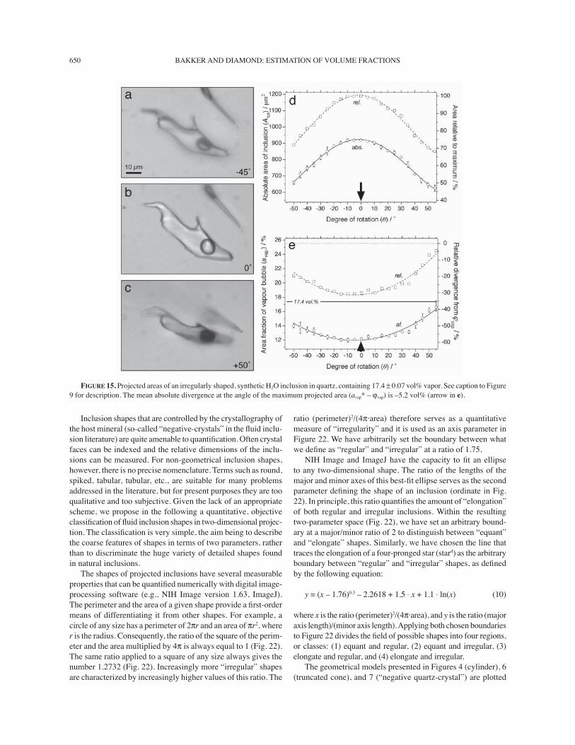
An irregular, slipper-shaped inclusion is shown in Figure 15. Similarly to Figure 12, the complexity of the shape does not allow the entire inclusion to be focused. The dashed Atot-θ curve in Figure 15d falls to 74% of its maximum upon 45° of rotation, approaching the behavior of a ß at inclusion (Fig. 8a), but the inclusion deÞ es comparison with any of the geometrical shapes modeled in Figures 4 to 7. All the values of avap markedly underestimate φvap (Figure 15e). In this case the reproducibility of the avap measurements is very good. There is no doubt that at θ* (0°), avap* underestimates φvap by 30% on the relative scale. This gross underestimation is comparable to that of the irregular-shaped inclusion in Figure 12.
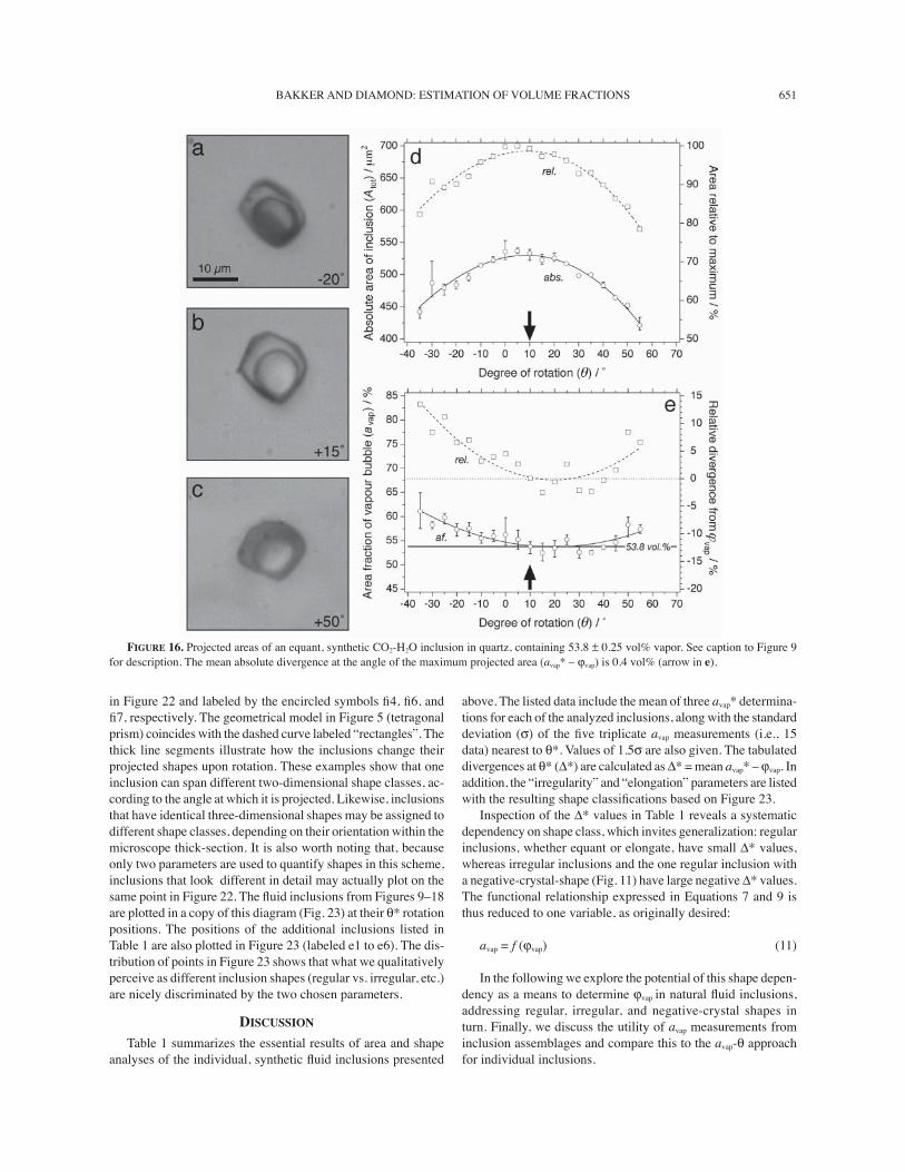
Measurements of individual synthetic CO2-H2O inclusions with 53.8% �vapor�
Figure 16 shows a highly equant inclusion. The dashed Atot-θ curve in Figure 16d falls to only around 80% of its maximum upon 45° of rotation, which in comparable to a cylinder with aspect ratio of 0.4, as shown in Figure 8a. Also the qualitative behavior of the avap-θ curves in Figure 16e is similar to the hypothetical cylinder modeled in Figure 4; at high angles of rotation, avap overestimates φvap by up to 14% on the relative scale. However, at θ* (10°) the mean value of avap* matches φvap perfectly.
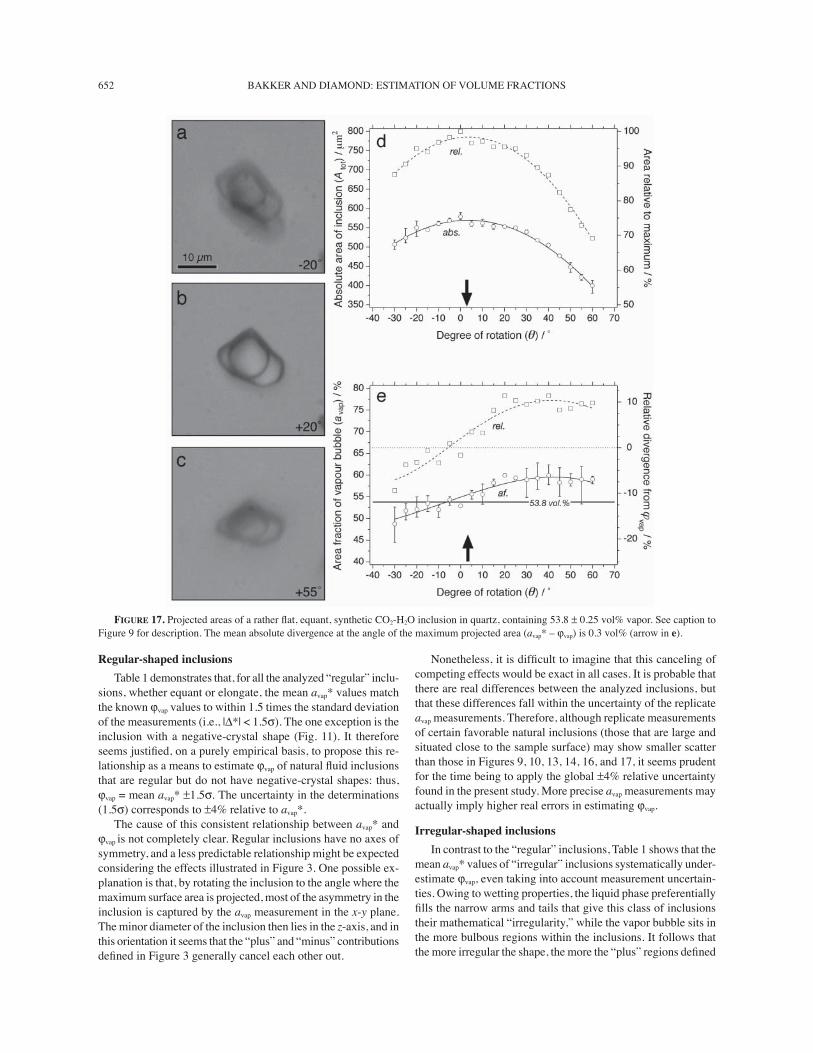
Figure 17 presents results for an essentially equant inclusion that is slightly elongated and ß attened compared to the inclusion in Figure 16. The long axis of the inclusion is oriented at about 30° to the rotation axis of the spindle stage. Similarly to Figure
FIGURE 12. Projected areas of an irregular shaped synthetic H2O inclusion in quartz, containing 67.8 vol% vapor. See caption to Figure 9 for description. (a) Inclusion at �60° rotation, photographed in one Þ xed plane of focus. (a') Scale drawing of the projected inclusion at �60° rotation, for which the focus of the microscope was optimized at each point on the inclusion perimeter. A similar scale drawing is illustrated for the +20° rotation (c and c'). (e) Filled symbols represent area fractions measured on scale drawings such as (a') and (c'). Open symbols show area fractions measured on photographs such as (a) and (c). The mean absolute divergence at the angle of the maximum projected area (avap* � φvap) is �13.6 vol% (solid arrow in e).
BAKKER AND DIAMOND: ESTIMATION OF VOLUME FRACTIONS648
13, strong double-refraction produces a blurred duplicate image in Figure 17a, hindering accurate measurement at higher angles of rotation. The form of the Atot-θ curves (Fig. 17d) is similar to that in Figure 16. The difference in shape is reß ected by the avap-θ curves (Fig. 17e), which are concave-down and which cut across the φvap line (cf. Fig. 16e). Nevertheless, the mean avap* (at θ* = 3°) is still a good estimate of φvap, exceeding the true value by only 3% on the relative scale.
Figure 18 summarizes measurements from one of the rarer irregular-shaped CO2-H2O inclusions. This inclusion displays only minor changes in projected area upon rotation between �20° and +30° (e.g., Figs. 18a and b), demonstrating that it actually has the shape of a club in three dimensions. The vapor bubble resides in the most equant portion of the inclusion (the head of the club). This broadly resembles the calculated geometrical models in which the bubble occupies the widest portion of elongate inclusions, such as curve b in Figure 6 (cone morphology) and curve c in Figure 7 (hexagonal prism). In contrast to the equant inclusions in this sample (Figs. 16 and 17), the avap-θ curves lie far below φvap. At θ* (13°), the mean avap* underestimates φvap
by �12% on the relative scale. This large negative divergence is strikingly similar to that found in the two other inclusions with highly irregular shapes: the �ladle� (Fig. 12) and the �slipper� (Fig. 15).
Measurements of assemblages of synthetic inclusions without rotation
Figures 19, 20, and 21 show the projected areas (Atot) vs. avap of large numbers of inclusions in the three synthetic samples. The measurements were made with the quartz disks in Þ xed horizontal positions (no rotation). Because all the inclusions in each sample were synthesized at the same experimental conditions, they all have essentially the same φvap at room temperature, regardless of the variation in their shapes and sizes.
Figure 19 (H2O inclusions with φvap = 67.8%) reveals a range of avap values between 56% and 77%, the scatter being indepen-dent of the apparent size (projected area) of the inclusions. The majority of the inclusions have avap values lower than φvap, but the mean of the data is 64.1%, which is quite close to φvap. In Figure 20 (CO2-H2O inclusions with φvap = 53.8 ± 0.25%) the smaller
FIGURE 13. Projected areas of an equant, synthetic H2O inclusion in quartz, containing 17.4 ± 0.07 vol% vapor. See caption to Figure 9 for description. Filled symbols represent measurements where double refraction created strong optical artifacts. These data were ignored during curve-Þ tting. The mean absolute divergence at the angle of the maximum projected area (avap* � φvap) is 1.2 vol% (arrow in e).
BAKKER AND DIAMOND: ESTIMATION OF VOLUME FRACTIONS 649
inclusions show a wide range of avap (between 45% and 64%) but the range is centered on φvap. The spread in avap decreases progressively as the size of the inclusions increases. The largest inclusions display avap values that only slightly underestimate φvap. It is noteworthy that the mean of all the 99 avap data is 53%, which again is very close to φvap.
The inclusions plotted in Figures 19 and 20 were chosen for measurement indiscriminately, without regard to shape or to the petrographically distinguishable assemblages in the samples. In contrast, the 89 inclusion measurements reported in Figure 21 (H2O inclusions with φvap = 17.4 ± 0.07%) are sorted according to assemblages: three healed fractures (each of which has a slightly different orientation within the sample), and a swarm of inclusions along the rim overgrowth of the quartz disk. The healed-fracture assemblages contain more or less regular inclusions, in which avap (varying between 16 and 25.9 vol%) tends to overestimate φvap (cf. Figs. 9, 10, 13, and 16). The rim assemblage contains regular and irregular inclusions, many of which are much larger than inclusions in the healed fractures. The avap values partly overestimate φvap (regular inclusions) and partly underestimate φvap (irregular inclusions), with a mean at 17.6%, which yet again is remarkably close to φvap.
Overall, these samples demonstrate that the mean avap of
assemblages consisting of small numbers of inclusions may signiÞ cantly overestimate φvap. It may be presumed, judging from the wide ranges of avap values observed, that the mean avap in other samples could just as easily underestimate φvap. How-ever, the mean avap values of very large numbers of cogenetic, homogeneously trapped inclusions yield good estimates of φvap (within ±4% on a relative scale).
DeÞ nition and classiÞ cation of ß uid inclusion shapes
The above results on individual inclusions show that rotation of inclusions to the position where their largest areas are projected largely accounts for the dependency of avap on inclusion orienta-tion. The functional relationship we are searching for (Eq. 7) is thus reduced by one variable:
avap = f (shape, φvap) (9)
The results also show a clear difference in behavior between regularly shaped and irregularly shaped inclusions and between elongate and equant inclusions. To quantify this dependency, an objective classiÞ cation of two-dimensional shapes is required, including reproducible boundaries between what we qualitatively term �regular,� �irregular,� �elongate,� and �equant.�
FIGURE 14. Projected areas of an elongate, synthetic H2O inclusion in quartz, containing 17.4 ± 0.07 vol% vapor. See caption to Figure 9 for description. The mean absolute divergence at the angle of the maximum projected area (avap* � φvap) is �0.6 vol% (arrow in e).
BAKKER AND DIAMOND: ESTIMATION OF VOLUME FRACTIONS650
Inclusion shapes that are controlled by the crystallography of the host mineral (so-called �negative-crystals� in the ß uid inclu-sion literature) are quite amenable to quantiÞ cation. Often crystal faces can be indexed and the relative dimensions of the inclu-sions can be measured. For non-geometrical inclusion shapes, however, there is no precise nomenclature. Terms such as round, spiked, tabular, tubular, etc., are suitable for many problems addressed in the literature, but for present purposes they are too qualitative and too subjective. Given the lack of an appropriate scheme, we propose in the following a quantitative, objective classiÞ cation of ß uid inclusion shapes in two-dimensional projec-tion. The classiÞ cation is very simple, the aim being to describe the coarse features of shapes in terms of two parameters, rather than to discriminate the huge variety of detailed shapes found in natural inclusions.
The shapes of projected inclusions have several measurable properties that can be quantiÞ ed numerically with digital image-processing software (e.g., NIH Image version 1.63, ImageJ). The perimeter and the area of a given shape provide a Þ rst-order means of differentiating it from other shapes. For example, a circle of any size has a perimeter of 2πr and an area of πr2, where r is the radius. Consequently, the ratio of the square of the perim-eter and the area multiplied by 4π is always equal to 1 (Fig. 22). The same ratio applied to a square of any size always gives the number 1.2732 (Fig. 22). Increasingly more �irregular� shapes are characterized by increasingly higher values of this ratio. The
ratio (perimeter)2/(4π·area) therefore serves as a quantitative measure of �irregularity� and it is used as an axis parameter in Figure 22. We have arbitrarily set the boundary between what we deÞ ne as �regular� and �irregular� at a ratio of 1.75.
NIH Image and ImageJ have the capacity to Þ t an ellipse to any two-dimensional shape. The ratio of the lengths of the major and minor axes of this best-Þ t ellipse serves as the second parameter deÞ ning the shape of an inclusion (ordinate in Fig. 22). In principle, this ratio quantiÞ es the amount of �elongation� of both regular and irregular inclusions. Within the resulting two-parameter space (Fig. 22), we have set an arbitrary bound-ary at a major/minor ratio of 2 to distinguish between �equant� and �elongate� shapes. Similarly, we have chosen the line that traces the elongation of a four-pronged star (star4) as the arbitrary boundary between �regular� and �irregular� shapes, as deÞ ned by the following equation:
y = (x � 1.76)0.3 � 2.2618 + 1.5 ⋅ x + 1.1 ⋅ ln(x) (10)
where x is the ratio (perimeter)2/(4π·area), and y is the ratio (major axis length)/(minor axis length). Applying both chosen boundaries to Figure 22 divides the Þ eld of possible shapes into four regions, or classes: (1) equant and regular, (2) equant and irregular, (3) elongate and regular, and (4) elongate and irregular.
The geometrical models presented in Figures 4 (cylinder), 6 (truncated cone), and 7 (�negative quartz-crystal�) are plotted
FIGURE 15. Projected areas of an irregularly shaped, synthetic H2O inclusion in quartz, containing 17.4 ± 0.07 vol% vapor. See caption to Figure 9 for description. The mean absolute divergence at the angle of the maximum projected area (avap* � φvap) is �5.2 vol% (arrow in e).
BAKKER AND DIAMOND: ESTIMATION OF VOLUME FRACTIONS 651
in Figure 22 and labeled by the encircled symbols Þ 4, Þ 6, and Þ 7, respectively. The geometrical model in Figure 5 (tetragonal prism) coincides with the dashed curve labeled �rectangles�. The thick line segments illustrate how the inclusions change their projected shapes upon rotation. These examples show that one inclusion can span different two-dimensional shape classes, ac-cording to the angle at which it is projected. Likewise, inclusions that have identical three-dimensional shapes may be assigned to different shape classes, depending on their orientation within the microscope thick-section. It is also worth noting that, because only two parameters are used to quantify shapes in this scheme, inclusions that look different in detail may actually plot on the same point in Figure 22. The ß uid inclusions from Figures 9�18 are plotted in a copy of this diagram (Fig. 23) at their θ* rotation positions. The positions of the additional inclusions listed in Table 1 are also plotted in Figure 23 (labeled e1 to e6). The dis-tribution of points in Figure 23 shows that what we qualitatively perceive as different inclusion shapes (regular vs. irregular, etc.) are nicely discriminated by the two chosen parameters.
DISCUSSION
Table 1 summarizes the essential results of area and shape analyses of the individual, synthetic ß uid inclusions presented
above. The listed data include the mean of three avap* determina-tions for each of the analyzed inclusions, along with the standard deviation (σ) of the Þ ve triplicate avap measurements (i.e., 15 data) nearest to θ*. Values of 1.5σ are also given. The tabulated divergences at θ* (Δ*) are calculated as Δ* = mean avap* � φvap. In addition, the �irregularity� and �elongation� parameters are listed with the resulting shape classiÞ cations based on Figure 23.
Inspection of the Δ* values in Table 1 reveals a systematic dependency on shape class, which invites generalization: regular inclusions, whether equant or elongate, have small Δ* values, whereas irregular inclusions and the one regular inclusion with a negative-crystal-shape (Fig. 11) have large negative Δ* values. The functional relationship expressed in Equations 7 and 9 is thus reduced to one variable, as originally desired:
avap = f (φvap) (11)
In the following we explore the potential of this shape depen-dency as a means to determine φvap in natural ß uid inclusions, addressing regular, irregular, and negative-crystal shapes in turn. Finally, we discuss the utility of avap measurements from inclusion assemblages and compare this to the avap-θ approach for individual inclusions.
FIGURE 16. Projected areas of an equant, synthetic CO2-H2O inclusion in quartz, containing 53.8 ± 0.25 vol% vapor. See caption to Figure 9 for description. The mean absolute divergence at the angle of the maximum projected area (avap* � φvap) is 0.4 vol% (arrow in e).
BAKKER AND DIAMOND: ESTIMATION OF VOLUME FRACTIONS652
Regular-shaped inclusions
Table 1 demonstrates that, for all the analyzed �regular� inclu-sions, whether equant or elongate, the mean avap* values match the known φvap values to within 1.5 times the standard deviation of the measurements (i.e., |Δ*| < 1.5σ). The one exception is the inclusion with a negative-crystal shape (Fig. 11). It therefore seems justiÞ ed, on a purely empirical basis, to propose this re-lationship as a means to estimate φvap of natural ß uid inclusions that are regular but do not have negative-crystal shapes: thus, φvap = mean avap* ±1.5σ. The uncertainty in the determinations (1.5σ) corresponds to ±4% relative to avap*.
The cause of this consistent relationship between avap* and φvap is not completely clear. Regular inclusions have no axes of symmetry, and a less predictable relationship might be expected considering the effects illustrated in Figure 3. One possible ex-planation is that, by rotating the inclusion to the angle where the maximum surface area is projected, most of the asymmetry in the inclusion is captured by the avap measurement in the x-y plane. The minor diameter of the inclusion then lies in the z-axis, and in this orientation it seems that the �plus� and �minus� contributions deÞ ned in Figure 3 generally cancel each other out.
Nonetheless, it is difÞ cult to imagine that this canceling of competing effects would be exact in all cases. It is probable that there are real differences between the analyzed inclusions, but that these differences fall within the uncertainty of the replicate avap measurements. Therefore, although replicate measurements of certain favorable natural inclusions (those that are large and situated close to the sample surface) may show smaller scatter than those in Figures 9, 10, 13, 14, 16, and 17, it seems prudent for the time being to apply the global ±4% relative uncertainty found in the present study. More precise avap measurements may actually imply higher real errors in estimating φvap.
Irregular-shaped inclusions
In contrast to the �regular� inclusions, Table 1 shows that the mean avap* values of �irregular� inclusions systematically under-estimate φvap, even taking into account measurement uncertain-ties. Owing to wetting properties, the liquid phase preferentially Þ lls the narrow arms and tails that give this class of inclusions their mathematical �irregularity,� while the vapor bubble sits in the more bulbous regions within the inclusions. It follows that the more irregular the shape, the more the �plus� regions deÞ ned
FIGURE 17. Projected areas of a rather ß at, equant, synthetic CO2-H2O inclusion in quartz, containing 53.8 ± 0.25 vol% vapor. See caption to Figure 9 for description. The mean absolute divergence at the angle of the maximum projected area (avap* � φvap) is 0.3 vol% (arrow in e).
BAKKER AND DIAMOND: ESTIMATION OF VOLUME FRACTIONS 653
in Figure 3 will dominate avap. This trend is borne out by the measurements plotted in Figure 23 for irregular inclusions with 67.8 and 53 vol% vapor. The closer the inclusions plot to the regular/irregular boundary, the smaller is the relative divergence between avap* and φvap; compare inclusions e4 (rel. Δ* = �4.3%) with e3 (�15%) and 18 (�12%) with e2 (�15%) and 12 (�19%). In fact, as indicated in Figure 23, the magnitude of Δ* appears to follow contours (labeled �10% and �20%) that lie parallel to the regular/irregular boundary. This systematic behavior suggests that the following rule could be applied: φvap = avap*+ Δ* ± 1.5σ. On the other hand, the slipper-shaped inclusion (number 15), which contains 17.4 vol% vapor, does not fall on the tentative contours in Figure 23. Although its relative Δ* is negative, its value is �30%, whereas the contours imply it should be approxi-mately �10%. It seems that the correction contours for irregular inclusions are a function of φvap itself, not just of inclusion shape. Although more experiments could be conducted to deÞ ne this function and to Þ t contours for a range of φvap values, it is not yet clear how this could be applied objectively to natural inclu-sions. Accordingly, we propose that the new method to estimate φvap should be applied only to regular inclusions, for which no additional Δ* correction is necessary.
Negative-crystal-shaped inclusions
The only measured regular inclusion that does not follow the rule of φvap = avap* ± 1.5σ happens to be the only inclusion with
FIGURE 18. Projected areas of an irregularly shaped, synthetic CO2-H2O inclusion in quartz, containing 53.8 ± 0.25 vol% vapor. See caption to Figure 9 for description. Dark blebs in the photographs of the inclusions are dust particles on the sample surface, not solid phases within the inclusions. The mean absolute divergence at the angle of the maximum projected area (avap* � φvap) is �6.3 vol% (arrow in e).
FIGURE 19. Projected area fractions vs. total areas of 60 synthetic H2O inclusions in quartz, each containing 67.8 vol% vapor (horizontal reference line). The measurements were made with the sample in a Þ xed orientation (no rotation). The mean area fraction is 64.1%.

BAKKER AND DIAMOND: ESTIMATION OF VOLUME FRACTIONS654
a shape that is strongly controlled by the crystallography of the host quartz (i.e., a �negative crystal�; Fig. 11). This result is as expected from the geometrical model in Figure 7, viewed from the angle of largest projected area (curve c in zones 2 and 3): the �plus� regions in Figure 3 strongly outweigh the �minus� regions when the inclusion is shaped like a negative quartz crystal with φvap > 25% (note that Fig. 3b itself corresponds to a b-type projection, for which avap > φvap). Unfortunately, the inclusion dimensions modeled in Figure 7 do not mimic inclu-sion 11 well, and consequently curve c overestimates the true φvap by 15% (relative). However, calculation of a new curve c speciÞ cally for the dimensions of inclusion 11 yields φvap = 68 to 70% for the measured mean avap* of 60%, which is acceptably close to the true φvap value of 67.8%. This example suggests that speciÞ c calculations such as those in Figures 5 and 7 could be used to estimate φvap for natural �regular� inclusions that exhibit crystallographically controlled faces. No universally applicable graphs for this problem are presented here.
Assemblages of ß uid inclusions
Figures 19 and 20 show that the mean of a large number of avap measurements is a reasonable estimate of φvap. The question arises as to whether the same approach could be applied to natural
FIGURE 20. Projected area fractions vs. total areas of 100 synthetic CO2-H2O inclusions in quartz, each containing 53.8 ± 0.25 vol% vapor (horizontal reference line). Measurements were made with the sample in a Þ xed orientation (no rotation). The mean area fraction is 53%.
FIGURE 21. Projected area fractions vs. total areas of 89 synthetic H2O inclusions in quartz, each containing 17.4 ± 0.07 vol% vapor (horizontal reference line). Measurements were made with the sample in a Þ xed orientation (no rotation). The inclusions are sorted according to petrographic assemblages. The mean area fraction of all 89 inclusions is 17.6%.
FIGURE 22. Objective shape-classification diagram for two-dimensional projections of ß uid inclusions. The abscissa shows the ratio of (perimeter)2/(4π·area), the ordinate shows the length ratio of major/minor axes of a best-Þ tting ellipse. Simple geometric shapes are plotted for reference. NA: not accessible. The intersection of the boundaries labeled �regular/irregular� and �equant/elongate� divides the Þ eld of accessible shapes into four arbitrary classes (shaded): equant and regular, elongate and regular, equant and irregular, elongate and irregular. Lines Þ 4, Þ 6, and Þ 7 represent the geometrical models illustrated in Figures 4, 6, and 7.
FIGURE 23. Objective shape-classiÞ cation diagram (see Figure 22 for description) showing positions of the synthetic ß uid inclusions analyzed in this study. Numbers 9 to 18 correspond to inclusions shown in Figures 9 to 18. Labels e1 to e6 are additional inclusions. Inclusions that plot in the regular classes and which do not have negative-crystal shapes (open circles) follow the rule φvap = avap* ± 4%. The one analyzed inclusion with a negative-crystal shape (number 11) is distinguished by a Þ lled hexagon. Inclusions that plot in the irregular classes (Þ lled circles) are labeled with their respective mean relative divergences (avap* � φvap) in vol%. These follow the rule φvap = avap* + Δ ± 4%, where the magnitude of Δ depends on distance from the regular/irregular boundary and on φvap. See text for further explanation.
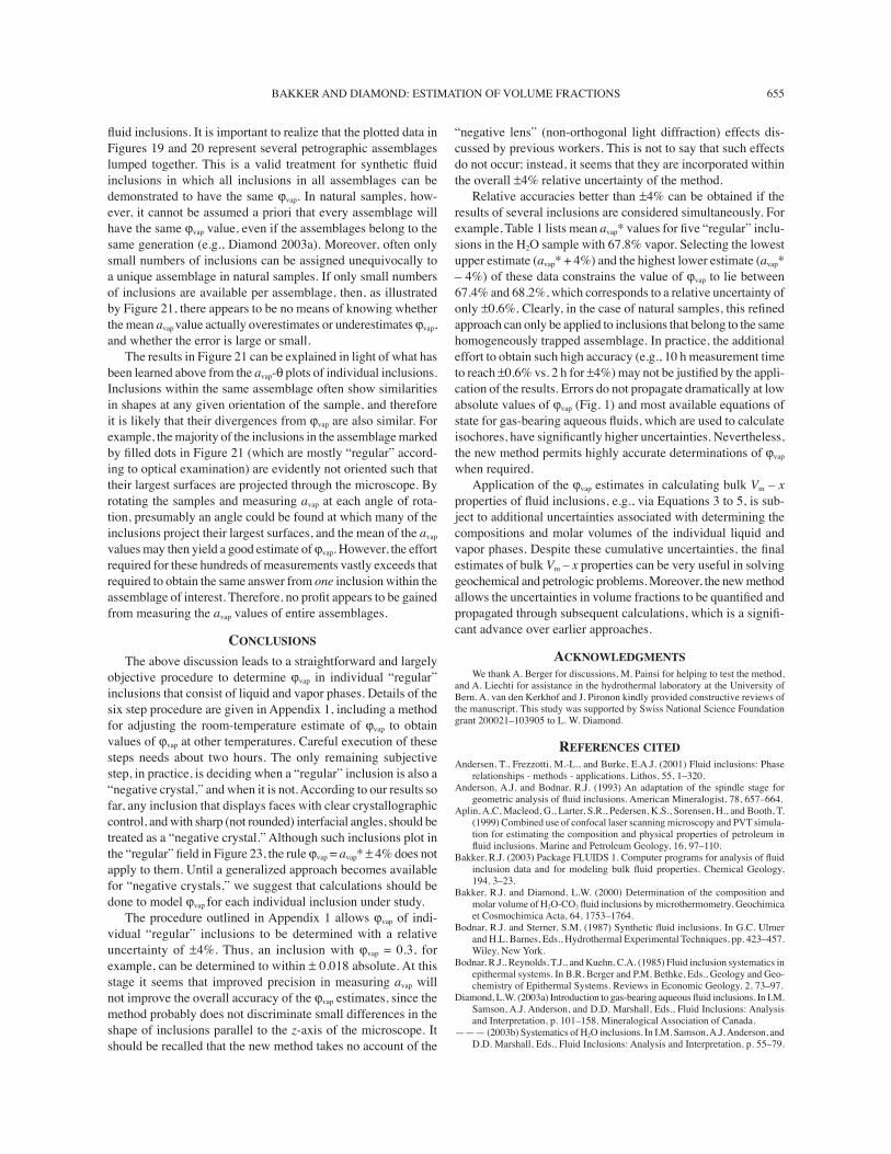
BAKKER AND DIAMOND: ESTIMATION OF VOLUME FRACTIONS 655
ß uid inclusions. It is important to realize that the plotted data in Figures 19 and 20 represent several petrographic assemblages lumped together. This is a valid treatment for synthetic ß uid inclusions in which all inclusions in all assemblages can be demonstrated to have the same φvap. In natural samples, how-ever, it cannot be assumed a priori that every assemblage will have the same φvap value, even if the assemblages belong to the same generation (e.g., Diamond 2003a). Moreover, often only small numbers of inclusions can be assigned unequivocally to a unique assemblage in natural samples. If only small numbers of inclusions are available per assemblage, then, as illustrated by Figure 21, there appears to be no means of knowing whether the mean avap value actually overestimates or underestimates φvap, and whether the error is large or small.
The results in Figure 21 can be explained in light of what has been learned above from the avap-θ plots of individual inclusions. Inclusions within the same assemblage often show similarities in shapes at any given orientation of the sample, and therefore it is likely that their divergences from φvap are also similar. For example, the majority of the inclusions in the assemblage marked by Þ lled dots in Figure 21 (which are mostly �regular� accord-ing to optical examination) are evidently not oriented such that their largest surfaces are projected through the microscope. By rotating the samples and measuring avap at each angle of rota-tion, presumably an angle could be found at which many of the inclusions project their largest surfaces, and the mean of the avap values may then yield a good estimate of φvap. However, the effort required for these hundreds of measurements vastly exceeds that required to obtain the same answer from one inclusion within the assemblage of interest. Therefore, no proÞ t appears to be gained from measuring the avap values of entire assemblages.
CONCLUSIONS
The above discussion leads to a straightforward and largely objective procedure to determine φvap in individual �regular� inclusions that consist of liquid and vapor phases. Details of the six step procedure are given in Appendix 1, including a method for adjusting the room-temperature estimate of φvap to obtain values of φvap at other temperatures. Careful execution of these steps needs about two hours. The only remaining subjective step, in practice, is deciding when a �regular� inclusion is also a �negative crystal,� and when it is not. According to our results so far, any inclusion that displays faces with clear crystallographic control, and with sharp (not rounded) interfacial angles, should be treated as a �negative crystal.� Although such inclusions plot in the �regular� Þ eld in Figure 23, the rule φvap = avap* ± 4% does not apply to them. Until a generalized approach becomes available for �negative crystals,� we suggest that calculations should be done to model φvap for each individual inclusion under study.
The procedure outlined in Appendix 1 allows φvap of indi-vidual �regular� inclusions to be determined with a relative uncertainty of ±4%. Thus, an inclusion with φvap = 0.3, for example, can be determined to within ± 0.018 absolute. At this stage it seems that improved precision in measuring avap will not improve the overall accuracy of the φvap estimates, since the method probably does not discriminate small differences in the shape of inclusions parallel to the z-axis of the microscope. It should be recalled that the new method takes no account of the
�negative lens� (non-orthogonal light diffraction) effects dis-cussed by previous workers. This is not to say that such effects do not occur; instead, it seems that they are incorporated within the overall ±4% relative uncertainty of the method.
Relative accuracies better than ±4% can be obtained if the results of several inclusions are considered simultaneously. For example, Table 1 lists mean avap* values for Þ ve �regular� inclu-sions in the H2O sample with 67.8% vapor. Selecting the lowest upper estimate (avap* + 4%) and the highest lower estimate (avap* � 4%) of these data constrains the value of φvap to lie between 67.4% and 68.2%, which corresponds to a relative uncertainty of only ±0.6%. Clearly, in the case of natural samples, this reÞ ned approach can only be applied to inclusions that belong to the same homogeneously trapped assemblage. In practice, the additional effort to obtain such high accuracy (e.g., 10 h measurement time to reach ±0.6% vs. 2 h for ±4%) may not be justiÞ ed by the appli-cation of the results. Errors do not propagate dramatically at low absolute values of φvap (Fig. 1) and most available equations of state for gas-bearing aqueous ß uids, which are used to calculate isochores, have signiÞ cantly higher uncertainties. Nevertheless, the new method permits highly accurate determinations of φvap when required.
Application of the φvap estimates in calculating bulk Vm � x properties of ß uid inclusions, e.g., via Equations 3 to 5, is sub-ject to additional uncertainties associated with determining the compositions and molar volumes of the individual liquid and vapor phases. Despite these cumulative uncertainties, the Þ nal estimates of bulk Vm � x properties can be very useful in solving geochemical and petrologic problems. Moreover, the new method allows the uncertainties in volume fractions to be quantiÞ ed and propagated through subsequent calculations, which is a signiÞ -cant advance over earlier approaches.
ACKNOWLEDGMENTSWe thank A. Berger for discussions, M. Painsi for helping to test the method,
and A. Liechti for assistance in the hydrothermal laboratory at the University of Bern. A. van den Kerkhof and J. Pironon kindly provided constructive reviews of the manuscript. This study was supported by Swiss National Science Foundation grant 200021�103905 to L. W. Diamond.
REFERENCES CITEDAndersen, T., Frezzotti, M.-L., and Burke, E.A.J. (2001) Fluid inclusions: Phase
relationships - methods - applications. Lithos, 55, 1�320.Anderson, A.J. and Bodnar, R.J. (1993) An adaptation of the spindle stage for
geometric analysis of ß uid inclusions. American Mineralogist, 78, 657�664.Aplin, A.C, Macleod, G., Larter, S.R., Pedersen, K.S., Sorensen, H., and Booth, T.
(1999) Combined use of confocal laser scanning microscopy and PVT simula-tion for estimating the composition and physical properties of petroleum in ß uid inclusions. Marine and Petroleum Geology, 16, 97�110.
Bakker, R.J. (2003) Package FLUIDS 1. Computer programs for analysis of ß uid inclusion data and for modeling bulk ß uid properties. Chemical Geology, 194, 3�23.
Bakker, R.J. and Diamond, L.W. (2000) Determination of the composition and molar volume of H2O-CO2 ß uid inclusions by microthermometry. Geochimica et Cosmochimica Acta, 64, 1753�1764.
Bodnar, R.J. and Sterner, S.M. (1987) Synthetic ß uid inclusions. In G.C. Ulmer and H.L. Barnes, Eds., Hydrothermal Experimental Techniques, pp. 423�457. Wiley, New York.
Bodnar, R.J., Reynolds, T.J., and Kuehn, C.A. (1985) Fluid inclusion systematics in epithermal systems. In B.R. Berger and P.M. Bethke, Eds., Geology and Geo-chemistry of Epithermal Systems. Reviews in Economic Geology, 2, 73�97.
Diamond, L.W. (2003a) Introduction to gas-bearing aqueous ß uid inclusions. In I.M. Samson, A.J. Anderson, and D.D. Marshall, Eds., Fluid Inclusions: Analysis and Interpretation, p. 101�158. Mineralogical Association of Canada.
��� (2003b) Systematics of H2O inclusions. In I.M. Samson, A.J. Anderson, and D.D. Marshall, Eds., Fluid Inclusions: Analysis and Interpretation, p. 55�79.
BAKKER AND DIAMOND: ESTIMATION OF VOLUME FRACTIONS656
Mineralogical Association of Canada.��� (2003c) Glossary: Terms and symbols used in ß uid inclusion studies. In I.M.
Samson, A.J. Anderson, and D.D. Marshall, Eds. Fluid Inclusions: Analysis and Interpretation, p. 363�372. Mineralogical Association of Canada.
Diamond, L.W. and AkinÞ ev, N.N. (2003) Solubility of CO2 in water from �1.5 to 100 °C and from 0.1 to 100 MPa: Evaluation of literature data and thermo-dynamic modeling. Fluid Phase Equilibria, 208, 263�288.
Pironon, J., Canals, M., Dubessy, J., Walgenwitz, F., and Laplace-Builhe, C. (1998) Volumetric reconstruction of individual oil inclusions by confocal scanning laser microscopy. European Journal of Mineralogy, 10, 1143�1150.
Roedder, E. (1967) Fluid inclusions as samples of ore ß uids. In H.L. Barnes, Ed., Geochemistry of Hydrothermal Ore Deposits, 515�574. Rinehard and Winston, New York.
��� (1972) Composition of ß uid inclusions. Geological Survey Professional Pa-per, 440-JJ, United States Government Printing OfÞ ce, Washington, pp. 164.
��� (1984) Fluid Inclusions, vol. 12. Reviews in Mineralogy, Mineralogical Society of America, Chantilly, Virginia.
Samson, I.M., Anderson, A.J., and Marshall, D.D. (2003) Fluid Inclusions: Analysis and Interpretation. Short Course 32. Mineralogical Association of Canada.
Saylor, C.P. (1965) A study of errors in the measurements of microscopic spheres. Applied Optics, 4, 477�486.
Shepherd, T.J., Rankin, A.H., and Alderton, D.H.M. (1985) A Practical Guide to Fluid Inclusion Studies. Blackie, Glasglow, U.K.
Wagner, W. and Pruss, A. (2002) The IAPWS formulation 1995 for the thermody-namic properties of ordinary water substance for general and scientiÞ c use. Journal of Physical and Chemical Reference Data, 31, 387�535.
MANUSCRIPT RECEIVED NOVEMBER 4, 2004MANUSCRIPT ACCEPTED MAY 2, 2005MANUSCRIPT HANDLED BY ALAN ANDERSON
APPENDIX 1: RECOMMENDED PROCEDURE TO MEASURE THE VOLUME FRACTION OF PHASES IN INDIVIDUAL
INCLUSIONS CONSISTING OF LIQUID AND VAPOR
Five steps are given below to determine the value of φvap at room temperature. A sixth step explains how to adjust this value to estimate φvap at other temperatures. It is assumed that the reader has studied the main body of this article.
Selection of target inclusions for measurement
Qualitative optical estimates of avap should be used, accord-ing to traditional practice, to distinguish homogeneous from heterogeneous entrapment of individual petrographic assem-blages. For homogeneously trapped inclusions, quantitative φvap determinations from only one to three inclusions per assemblage are sufÞ cient, in principle, to deÞ ne φvap. For heterogeneously trapped inclusions, more measurements may have to be made per assemblage to Þ nd the extreme values of φvap in the liquid-rich and gas-rich end-members (e.g., Diamond 2003b). For both homogeneously and heterogeneously trapped assemblages, optimal inclusions for measurement are (1) large (the errors in measuring avap are minimized), (2) regular in shape (irregular inclusions cannot be quantiÞ ed with the current methodology), and (3) situated near the surface of the sample (the clarity of inclusions upon rotation is maximized).
Rotation of inclusion samples
Mount the sample on the spindle stage and center the axis of rotation on the target inclusion. Using the highest microscope magniÞ cation possible (usually a 36× or a 40× long working-distance objective lens), take digital photographs of the inclu-sion at 5° intervals of rotation (+ and �), over as large a range of angles as permitted by the clarity of the images. Record the orientation of the spindle-stage axis and the length scale (in μm) of the photographs (for routine analysis, pixels are sufÞ cient).
For each photograph, record the angle of rotation. Use a polarizer below the sample to reduce double refraction at high angles of rotation. For inclusions that are not entirely focused at a given position, photographs are unsuitable for area measurements. Better accuracy is obtained by making a drawing of the inclusion while optimizing the focus at each point along the perimeters of the inclusion and the vapor bubble. Drawings can be made using a projection tube mounted on the microscope or by tracing on a clear plastic sheet placed over the inclusion image displayed on a computer screen.
Measurement of Atot and avap
Import the digital photographs or scanned drawings into ImageJ (freeware obtainable at http://rsb.info.nih.gov/). Use the Polygon Selections tool to measure the length scale of the photograph in pixels. Then within the Analyze menu, select the Set Scale option and enter this pixel length to deÞ ne the scale of the photographs (typically around 6 pixel/μm for a 40× objective lens). In the Set Measurement option, select the parameters for measurement (Area, Perimeter, Fit Ellipse) and specify their precision to three decimal places. For each image, use the Polygon Selection tool to draw around the perimeter of the inclusion, then from the Analyze menu execute Measure to record the values of the parameters. Repeat the measurements for the vapor bubble. Care must be taken to trace around the outside edges of the dark shadows that deÞ ne the inclusion and bubble perimeters; these correspond most closely to the true projection of the inclusion. To enhance accuracy, the measurements should be repeated at least thrice; we recommend tracing once clockwise then once anticlockwise, then the image should be enlarged to 200% and traced again. Calculate the area fraction of the vapor (avap) for each image.
Initial Estimate of avap
Plot the inclusion areas, Atot, and the calculated avap values as a function of rotation angle θ, as shown in Figures 9 to 18. Fit the data sets to polynomial functions by least-squares re-gression. If the Atot-θ function displays a maximum, locate the corresponding avap value at this angle. This particular value of avap is denoted avap*. For a range of angles near avap* (e.g., the Þ ve nearest sets of triplicate avap measurements, corresponding to 15 data), calculate the local standard deviation (σ) of avap with respect to the polynomial Þ t. This procedure yields the initial estimate (avap* ± σ).
Discrimination of inclusion shapes and estimation of φvap
Spherical inclusions. If the Þ tted Atot-θ function is ß at, the inclusion is spherical, and so the avap-θ function should also be essentially constant. In this case, a selection of the Þ ve triplicate sets of avap measurements that were made under the best observa-tion conditions (clarity of inclusion and bubble outlines) can be used to calculate the mean and standard deviation of avap. The resulting mean avap ± σ can now be plotted on curve s in Figure 4 to determine φvap ± σ.
Flat inclusions. The inclusion can be identiÞ ed as being ß at if (1) the avap-θ curve is nearly constant and (2) the Atot-θ curve is closely described by the function Atot = 100·cosθ over at least 45° of rotation (i.e., Atot falls to 71% of its maximum

BAKKER AND DIAMOND: ESTIMATION OF VOLUME FRACTIONS 657
upon 45° of rotation). If these two criteria are fulÞ lled, then φvap = avap* ± σ.
�Negative-crystal� inclusions. Examine the photographs to identify whether the inclusion shape is strongly controlled by the crystallography of the host mineral. Such �negative-crystals� have straight facet outlines in projection, and sharp (not rounded) interfacial angles. Inclusion outlines that are only partly faceted in this way also qualify for the present purposes as negative crystals (cf. Fig. 11). Calculate the theoretical volume of the inclusion by assuming it to be a perfect geometrical body (e.g., hexagonal prism with pyramids for quartz; cube for ß uorite) with outer dimensions as observed in the series of photographs. For elongate negative-crystal shapes, identify the maximum angle between the longest axis of the inclusion and the rotation axis of the spindle stage (αmax, see also Fig 8c and d). Taking the geometrical effect of αmax into account, calculate theoretical avap* values for a range of model φvap values and plot them in a new avap*-φvap curve, similar to c in Figure 7. The measured mean avap* ± σ can now be plotted on the new curve to obtain φvap ± σ of the inclusion.
Other inclusion shapes (i.e., those that are not spherical, ß at, or negative-crystals)
Using the Area, Perimeter, and Fit Ellipse measurements performed in step 4, plot the position of the inclusion on the shape-classiÞ cation diagram (Fig. 23). For all inclusions that fall in the regular Þ eld (whether elongate or equant; Eq. 10), check that 1.5σ < (avap* ± 4%). If so, the recommended global uncertainty of ±4% (relative to avap*) can be applied with con-Þ dence; thus φvap = avap* ± 4%. If 1.5σ > (avap* ± 4%), which
reß ects optical conditions worse than those found in the present study, the best estimate to use is φvap = avap* ± 1.5σ. Inclusions that plot in the irregular Þ eld cannot be analyzed accurately with the present methodology.
Estimation of φvap at temperatures above or below room temperature
The current design of the spindle stage (Anderson and Bod-nar 1993) does not permit inclusions to be heated or cooled; all measurements must be performed at room temperature. If φvap is required at another temperature (e.g., to perform calculations of bulk Vm � x properties), then the room-temperature estimate of φvap obtained using the above method can be roughly adjusted by measuring the change in radius (r) of the vapor bubble between room temperature (T1) and the target temperature (T2). Thus, for a spherical bubble (assuming that the volume of the total inclu-sion remains constant):
ϕ ϕvap vapvap
vap
T Tr T
r T2 1
23
13( ) = ( )⋅
( )( )
⎛
⎝
⎜⎜⎜⎜⎜
⎞⎞
⎠
⎟⎟⎟⎟⎟ (A1)
For example, if φvap(20 °C) = 0.2 and rvap(20 °C) = 4 μm, and if the radius of the spherical bubble increases to 5 μm upon cooling to �20 °C, then φvap(�20 °C) = 0.2 · (53 / 43) = 0.39. Similarly, for a ß at bubble:
ϕ ϕvap vapvap
vap
T Tr T
r T2 1
22
12( ) = ( )⋅
( )( )
⎛
⎝
⎜⎜⎜⎜⎜
⎞⎞
⎠
⎟⎟⎟⎟⎟ (A2)
For deformed bubbles with shapes between spherical and ß at, no simple solution is offered other than the upper and lower bounds imposed by Equations 12 and 13.