ESTIMATION OF TIME TO MAXIMUM RATE UNDER ADIABATIC CONDITIONS

(TMRad) USING KINETIC PARAMETERS DERIVED FROM DSC - INVESTIGATION OF

THERMAL BEHAVIOR OF 3-METHYL-4-NITROPHENOL

Bertrand Roduit1, Patrick Folly

2, Alexandre Sarbach

2, Beat Berger

2, Franz Brogli

3, Francesco

Mascarello4, Mischa Schwaninger

4, Thomas Glarner

5, Eberhard Irle

6, Fritz Tobler

6, Jacques Wiss

7,

Markus Luginbühl8, Craig Williams

8, Pierre Reuse

9, Francis Stoessel

9

1AKTS AG, TECHNOArk 1, 3960 Siders, Switzerland, http://www.akts.com, b.roduit@akts.com

2armasuisse, Science and Technology Centre, 3602 Thun, Switzerland

3Ciba Schweizerhalle AG, P.O. Box, 4002 Basel, Switzerland

4DSM Nutritional Products Ltd., Safety laboratory, 4334 Sisseln, Switzerland

5F. Hoffmann-La Roche Ltd, Safety laboratories, 4070 Basel, Switzerland

6Lonza AG, Safety Laboratory Visp, Rottenstr. 6, 3930 Visp, Switzerland

7Novartis Pharma AG, Novartis Campus, WSJ-145.8.54, 4002 Basel, Switzerland

8Syngenta Crop Protection Münchwilen AG, WMU 3120.1.54, 4333 Münchwilen, Switzerland

9Swiss Safety Institute, Schwarzwaldallee 215, WRO-1055.5.02, 4002 Basel, Switzerland

ABSTRACT

Kinetic parameters of the decomposition of hazardous chemicals can be applied for the

estimation of their thermal behavior under any temperature profile. Presented paper describes the

application of the advanced kinetic approach for the determination of the thermal behavior also under

adiabatic conditions occurring e.g. in batch reactors in case of cooling failure.

The kinetics of the decomposition of different samples (different manufacturers and batches) of 3-

methyl-4-nitrophenol were investigated by conventional DSC in non-isothermal (few heating rates

varying from 0.25 to 8.0 K/min) and isothermal (range of 200-260°C) modes. The kinetic parameters

obtained with AKTS-Thermokinetics Software were applied for calculating reaction rate and

progress under different heating rates and temperatures and verified by comparing simulated and

experimental signals. After application of the heat balance to compare the amount of heat generated

during reaction and its removal from the system, the knowledge of reaction rate at any temperature

profiles allowed the determination of the temperature increase due to the self-heating in adiabatic and

pseudo-adiabatic conditions.

Applied advanced kinetic approach allowed simulation the course of the Heat-Wait-Search (HWS)

mode of operation of adiabatic calorimeters. The thermal safety diagram depicting dependence of

Time to Maximum Rate (TMR) on the initial temperature was calculated and compared with the

results of HWS experiments carried out in the system with Φ-factor amounting to 3.2. The influence

of the Φ-factor and reaction progress reached at the end of the HWS monitoring on the TMR is

discussed. Presented calculations clearly indicate that even very minor reaction progress reduces the

TMRad of 24 hrs characteristic for a sample with initial reaction progress amounting to zero.

Described estimation method can be verified by just one HWS-ARC, or by one correctly chosen

ISO-ARC run of reasonable duration by knowing in advance the dependence of the TMR on the

initial temperature for any Φ-factor. Proposed procedure results in significant shortening of the

measuring time compared to a safety hazard approach based on series of ARC experiments carried

out at the beginning of a process safety evaluation.

Keywords: Adiabatic Conditions, Methyl, Nitrophenol, DSC, Φ-Factor, Kinetics, Thermal Runaway, Time to Maximum Rate (TMR)

INTRODUCTION

Differential Scanning Calorimetry (DSC) (1-3) and Accelerating Rate Calorimetry (ARC) (4-

9) are often used for the precise determination of the heat flow generated (or consumed) by a sample

during experiments carried out in non-isothermal or isothermal (DSC), adiabatic or pseudo-adiabatic

conditions (ARC). In the DSC technique the heating rate, being the very important experimental

parameter, is arbitrarily chosen by the user, in contrary, in ARC, the temperature increase during

exothermic reactions results from the self-heating of the material.

The runaway reactions are generally investigated by the time-consuming ARC experiments or

in isothermal (ISO-ARC) or heat-wait-search (HWS) modes. In the present paper we discuss the

application of the DSC traces after advanced kinetic analysis for the determination of the Time to

Maximum Rate under adiabatic conditions (TMRad) and simulation of the course of ARC

experiments performed in both modes. We propose an advanced kinetic elaboration of the DSC data

which allows constructing link between the results collected in different experimental conditions:

(i) DSC signals recorded in non-isothermal conditions (constant temperature rise) using

heating rates in the range generally between 0.25- 10 K/min

(ii) Isothermal DSC data obtained at different temperatures (heating rate amounts to 0

K/min)

(iii) ARC data obtained from adiabatic (Φ=1) or pseudo-adiabatic conditions (Φ＞1) in

which the temperature rise changes progressively from zero to several K/min due to

the sample self-heating. This process depends mainly on the kinetics of the

decomposition, adiabatic temperature rise, Cp of the sample and Φ-factor.

The key factor allowing the simulation of the reactions course under any temperature mode is the

knowledge of the kinetic parameters depicting the dependence of the rate of heat evolution on

different heating rates. These kinetic parameters are calculated from the non-iso or isothermal signals

using advanced kinetic analysis based on the differential isoconversional approach (10-13).

Isoconversional methods of the kinetic determination are based on the assumptions that the reaction

rate dα/dt for a given reaction progress α is only a function of the temperature. This assumption is

valid for most of the decomposition reactions but as it is not an axiom it needs to be verified in each

analysis. If the isoconversional assumption is valid, the calculated kinetic parameters can be applied

for simulating the reaction rate at any temperature change mode such as:

(i) ‘non-isothermal’ (constant heating rate)

(ii) ‘isothermal’ (constant temperature)

(iii) ‘adiabatic’ (progressive temperature rise due to ‘self-heating’ of the sample)

Depending on the type of technique and experimental set-up e.g. non-isothermal or isothermal DSC,

HWS or ISO-ARC, the process of data collection can be more or less time consuming.

Below we propose the optimization of the experimental procedure which will be illustrated by the

prediction of the TMR value for the 3-methyl-4-nitrophenol (MN), CAS No: 2581-34-2, using the

results collected in a round robin test in which few participants have investigated the different

batches of MN in different calorimeters using company specific experimental set-ups. In the

procedure proposed by us all non-iso and isothermal data delivered by the participants of the test

were used for the determination of the kinetic parameters of the reaction of the MN decomposition

and the heat of the reaction ∆Hr. The correctness of the procedure of the determination of kinetic

parameters was verified by the comparison of the experimental and simulated signals. The DSC

derived kinetic parameters were applied for the simulation of the adiabatic experiments.

EXPERIMENTAL

For the determination of the kinetic parameters of the decomposition of MN originating from

different suppliers and different batches, the DSC technique was applied. Different DSC apparatus

from various manufacturers were used. The measured data were subsequently exported in ASCII

format and elaborated with AKTS-Thermokinetics Software. The decomposition of the MN was

investigated in non-iso experiments in the range of 20°C to 350°C at different heating rates of 0.25,

0.5, 1, 2, 4 and 8 K/min and, isothermally, at temperatures 200, 210, 220, 230, 240, 250 and 260°C.

All experiments were performed in gold plated high pressure sealed crucibles (14) with a sample

mass varying between 4.8 and 12.22 mg.

RESULTS AND DISCUSSION

DSC DATA- ELABORATION AND SIMULATION

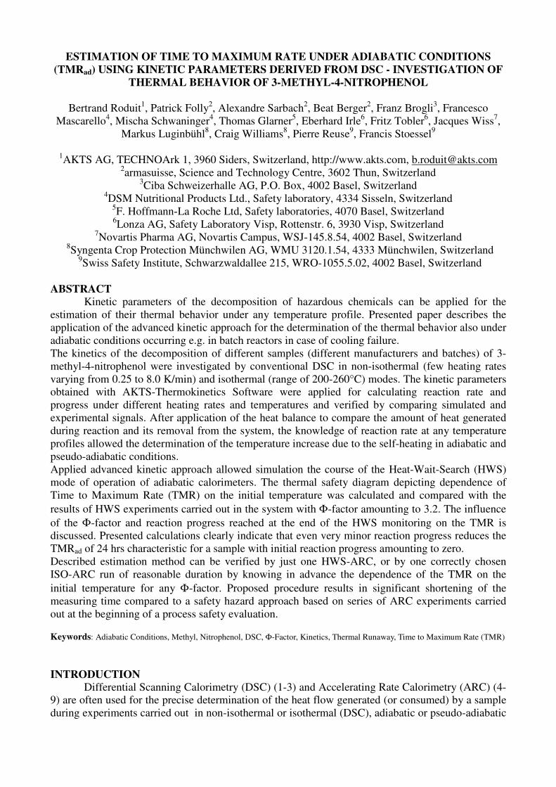
The typical DSC signal of MN recorded in non-isothermal conditions is presented in Figure 1

(top). After endothermic melting (maximum of endo-peak centred at 128.2°C, the sample starts to

decompose.

Temperature (°C)

325300275250225200175150125

HeatF

low

(W

/g)

5

4

3

2

1

0

-1

-2

-3

-4

ExoHeat : -2,194.016 (J/g)

T : 198.92 and 344.13 (°C)

Top of Peak : 294.34 (°C)

Peak Height : 4.41 (W/g)

Baseline Type : Tangential Sigmoid

128.16 (°C)

.

Temperature (°C)

340320300280260240220200

Reaction r

ate

(-/

s)

2E-3

1.5E-3

1E-3

5E-4

0

. Figure 1. (Top) Typical DSC trace of 3-methyl-4-nitrophenol recorded at 4 K/min and sigmoid baseline construction.

(Bottom) The reaction rates for all samples at 4K/min. Despite of the different experimental setups and sample origins

the reproducibility of the DSC traces is acceptable.

For the depicted sample, analysed with the heating rate of 4 K/min, the maximum of the exo-peak is

centred at 294.3°C. With the applied sigmoid-type baseline the determined reaction heat and

temperatures of the beginning and the end of the decomposition amount to about -2194 J/g; 199°C

and 344°C, respectively. In order to present the results for all samples in one diagram (Figure 1,

bottom) they are normalized and the reaction course is displayed as the dependence of the reaction

rate (rate of the change of the reaction progress α varying between 0 and 1 at the beginning and the

reaction end, respectively) on the temperature.

The comparison of the DSC traces recorded for different samples on different calorimeters at the

same heating rate of 4 K/min (Figure 1, bottom) shows quite high reproducibility of the results.

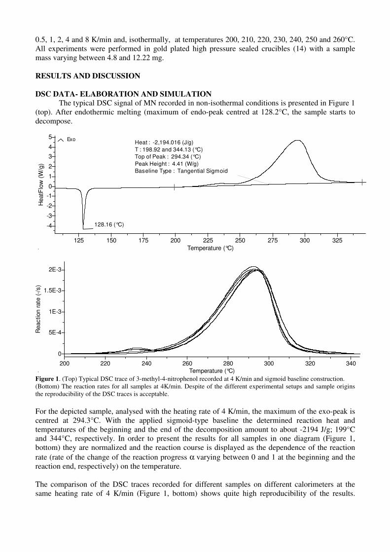
Experimental discrepancy between the curves concerns mainly the occurrence of a small thermal

event in the region of the detected decomposition onset as well as the temperature of the exothermal

event. All data collected in non-isothermal and isothermal experiments are displayed in Figure 2.

Temperature (°C)

340320300280260240220200

Reaction r

ate

(-/

s)

0.003

0.002

0.001

0

Reaction p

rogre

ss (

-)

1

0.8

0.6

0.4

0.2

0

1

.

.

2

4

8

0.50.25

4

0.25

0.5

1

24

8

4

.

Time (h)

1614121086420

Reaction r

ate

(-/

s)

6E-4

5E-4

4E-4

3E-4

2E-4

1E-4

0

Reaction p

rogre

ss (

-)

1

0.8

0.6

0.4

0.2

0

240

260

250

190

230

220

210

200

190200210

220

230

240

250

260

.

.

220

220

. Figures 2. Reaction rates dα/dt and progresses α corresponding to the normalized DSC-signals for the decomposition of

all 3-methyl-4-nitrophenol samples under non-isothermal (top) and isothermal (bottom) conditions. The values of the

heating rates and temperatures are marked on the curves. The comparison of the experimental and simulated signals at

chosen experimental conditions is shown in the respective insets.

The simulation of the experimental data (see insets in Figure 2) requires the determination of the

kinetic parameters of the decomposition reaction. It was done applying a differential isoconversional

method based on Friedman approach (15).

The reaction rate can be expressed as

( ) ( )( )( )

))

1exp(·

T(tR

EfA

dt

d ααα

α−= (1)

where t, T(t), E(α) and A(α) are the time, temperature, apparent activation energy and preexponential

factor at conversion α, respectively. In logarithmic form one can write:

( ) ( )( )( )

)

1·lnln

T(tR

EfA

dt

d ααα

α−=

(2)

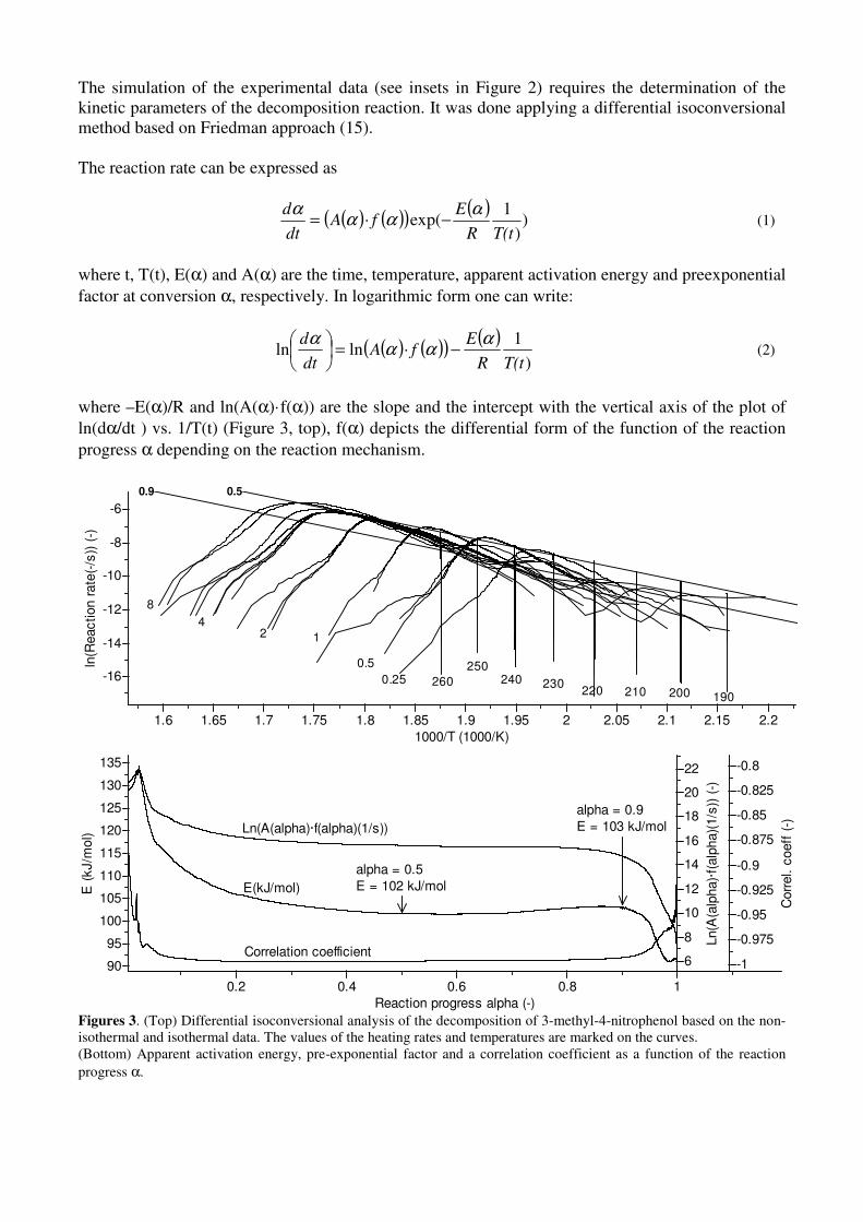
where –E(α)/R and ln(A(α)·f(α)) are the slope and the intercept with the vertical axis of the plot of

ln(dα/dt ) vs. 1/T(t) (Figure 3, top), f(α) depicts the differential form of the function of the reaction

progress α depending on the reaction mechanism.

1000/T (1000/K)

2.22.152.12.0521.951.91.851.81.751.71.651.6

ln(R

eaction r

ate

(-/s

)) (

-)

-6

-8

-10

-12

-14

-16 0.25

0.50.9

0.5

124

8

190200210220230240

250

260

Reaction progress alpha (-)

10.80.60.40.2

E (

kJ/m

ol)

135

130

125

120

115

110

105

100

95

90

Ln(A

(alp

ha)·

f(alp

ha)(

1/s

)) (

-)

22

20

18

16

14

12

10

8

6

Corr

el. c

oeff

(-)

-0.8

-0.825

-0.85

-0.875

-0.9

-0.925

-0.95

-0.975

-1

Ln(A(alpha)·f(alpha)(1/s))

alpha = 0.9

E = 103 kJ/mol

alpha = 0.5

E = 102 kJ/mol E(kJ/mol)

Correlation coefficient

Figures 3. (Top) Differential isoconversional analysis of the decomposition of 3-methyl-4-nitrophenol based on the non-

isothermal and isothermal data. The values of the heating rates and temperatures are marked on the curves.

(Bottom) Apparent activation energy, pre-exponential factor and a correlation coefficient as a function of the reaction

progress α.

The logarithm of the reaction rates is presented as a function of the reciprocal temperature for the

different temperatures and heating rates (Figure 3, top). The differential isoconversional analysis

allows finding the Arrhenius dependence for any, arbitrarily chosen decomposition progress α. The

slope of this dependence gives the apparent activation energy and preexponential factor at each stage

of the decomposition progress α (Figure 3, bottom). For example we see that for a reaction progress

α of 0.5 the apparent activation energy amounts to about 102 kJ/mol and for α= 0.9 the apparent

activation energy is only slightly larger (different slope) and amounts to ca. 103 kJ/mol.

The construction of the baseline of the DSC signal (Figure 1, top) plays an important role in the

correct determination of the reaction progress which is based on the integration of the DSC signals

area. Incorrect baseline construction influences the integral intensity of the signal what leads to the

incorrect determination of the reaction progress what, in turn, influences the values of the kinetic

parameters. In order to optimize the determination of the kinetic parameters from DSC traces in

AKTS-Thermokinetics Software Version 3 the reaction range is divided into numerous intervals and

the evaluation of the apparent activation energy E(α) and preexponential factor A(α)·f(α) is carried

out for each differential reaction progress α. In an ideal situation, i.e. without experimental noise and

with the isoconversional assumption holding in 100%, the average value of all correlation

coefficients of all straight lines obtained in the coordinates expressed in the eq.2 and depicted in

Figure 3 (top) should reach the best value of ‘-1’. AKTS-Thermokinetics Software applies non-linear

numerical analysis for baseline optimization to reach that best value by adjusting the tangents used

for the constructions of all sigmoid baselines. The average value of all regression coefficients is a

measure of the quality of the experimental data (level of experimental noise, correctness of baseline

construction, correct choice of the temperature in the isothermal experiments, etc.) and the

correctness of the assumption concerning the isoconversional principle stating that the reaction rate

depends only on the temperature. The optimized adjustment of the baseline changes additionally the

standard deviation of the value of the reaction heat ∆Hr. The mean value of the ∆Hr was measured

from the DSC traces by calculating the average of the values measured at different heating rates

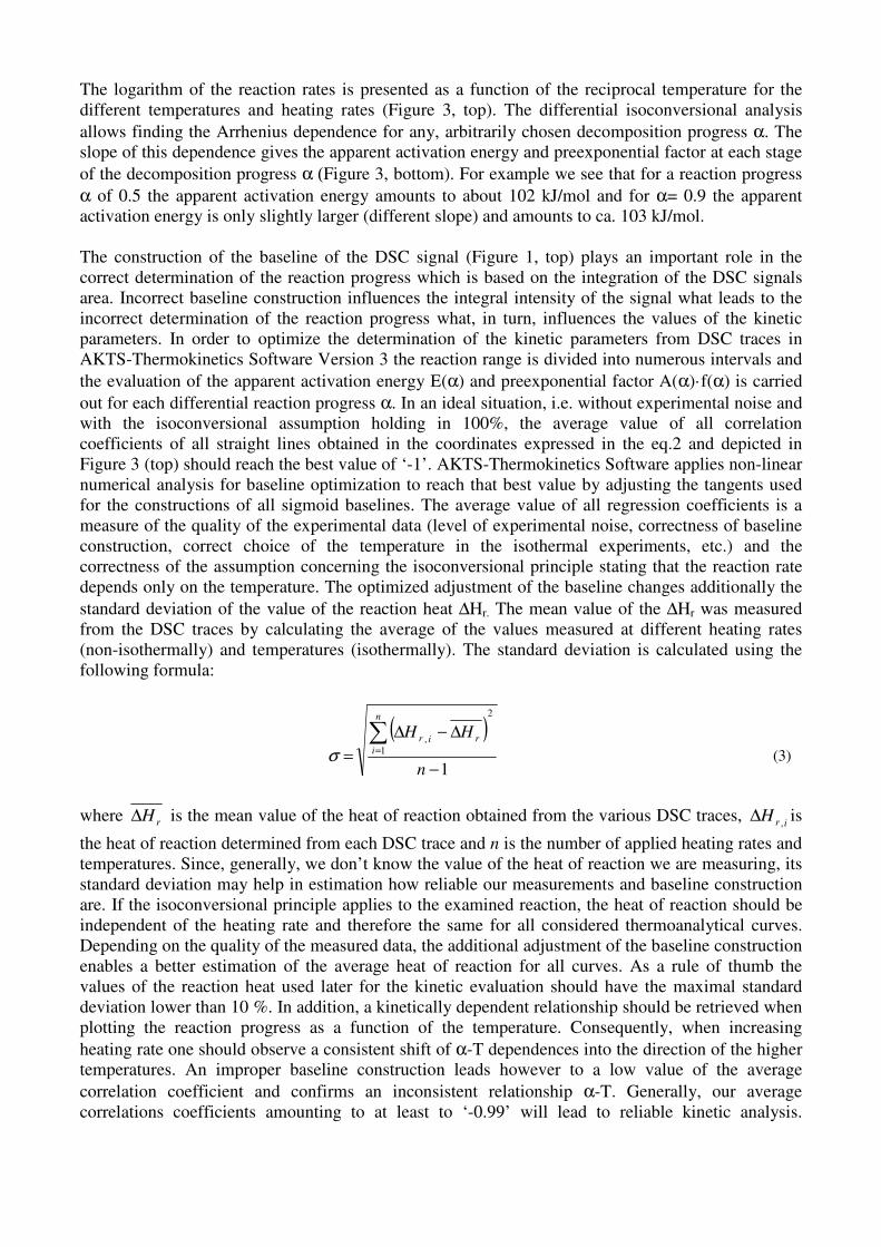
(non-isothermally) and temperatures (isothermally). The standard deviation is calculated using the

following formula:

( )

1

2

1,

−

∆−∆

=

∑=

n

HHn

i

rir

σ (3)

where rH∆ is the mean value of the heat of reaction obtained from the various DSC traces, irH

,∆ is

the heat of reaction determined from each DSC trace and n is the number of applied heating rates and

temperatures. Since, generally, we don’t know the value of the heat of reaction we are measuring, its

standard deviation may help in estimation how reliable our measurements and baseline construction

are. If the isoconversional principle applies to the examined reaction, the heat of reaction should be

independent of the heating rate and therefore the same for all considered thermoanalytical curves.

Depending on the quality of the measured data, the additional adjustment of the baseline construction

enables a better estimation of the average heat of reaction for all curves. As a rule of thumb the

values of the reaction heat used later for the kinetic evaluation should have the maximal standard

deviation lower than 10 %. In addition, a kinetically dependent relationship should be retrieved when

plotting the reaction progress as a function of the temperature. Consequently, when increasing

heating rate one should observe a consistent shift of α-T dependences into the direction of the higher

temperatures. An improper baseline construction leads however to a low value of the average

correlation coefficient and confirms an inconsistent relationship α-T. Generally, our average

correlations coefficients amounting to at least to ‘-0.99’ will lead to reliable kinetic analysis.

Therefore, to avoid improper baseline construction and achieve reliable analyses three procedures

can be applied:

- slight modification of the tangents at the beginning or at the end of the signals

- minor change of the temperature range of the selected of thermal analysis curves

- new measurements when necessary.

In the current study, the average value of all correlation coefficients amounts to -0.9928 and the

mean reaction heat ∆Hr to -2001.7±216.5 J/g. Deviation of the average regression coefficient from its

maximal value and relatively large standard deviation of the ∆Hr value result mainly from the

experimental error i.e. the not optimal choice of temperatures in isothermal mode of the

investigations. At too high isothermal temperatures (as 250 and 260°C) the significant part of the

data collected at the beginning of the decomposition is not fully applicable in kinetic analysis. Due to

the time required for the temperature settling in the sample, some part of the decomposition (as larger

as temperature is higher) occurs at temperatures lower than set. Also, if the reactions rate are high,

the problem of the time constant of the measuring sensors - see e.g. in (16,17) - starts to play an

important role in the correct evaluation of the thermograms. These remarks are illustrated by the

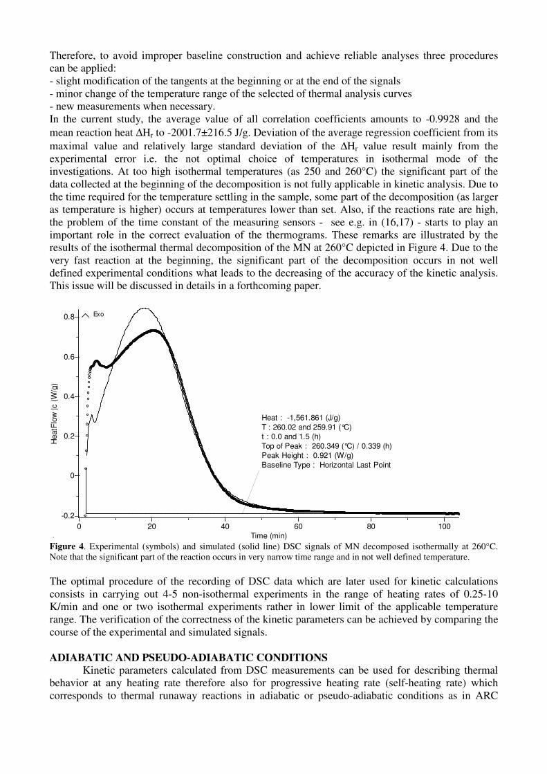
results of the isothermal thermal decomposition of the MN at 260°C depicted in Figure 4. Due to the

very fast reaction at the beginning, the significant part of the decomposition occurs in not well

defined experimental conditions what leads to the decreasing of the accuracy of the kinetic analysis.

This issue will be discussed in details in a forthcoming paper.

Time (min)

100806040200

HeatF

low

|c (

W/g

)

0.8

0.6

0.4

0.2

0

-0.2

Exo

Heat : -1,561.861 (J/g)

T : 260.02 and 259.91 (°C)

t : 0.0 and 1.5 (h)

Top of Peak : 260.349 (°C) / 0.339 (h)

Peak Height : 0.921 (W/g)

Baseline Type : Horizontal Last Point

. Figure 4. Experimental (symbols) and simulated (solid line) DSC signals of MN decomposed isothermally at 260°C.

Note that the significant part of the reaction occurs in very narrow time range and in not well defined temperature.

The optimal procedure of the recording of DSC data which are later used for kinetic calculations

consists in carrying out 4-5 non-isothermal experiments in the range of heating rates of 0.25-10

K/min and one or two isothermal experiments rather in lower limit of the applicable temperature

range. The verification of the correctness of the kinetic parameters can be achieved by comparing the

course of the experimental and simulated signals.

ADIABATIC AND PSEUDO-ADIABATIC CONDITIONS

Kinetic parameters calculated from DSC measurements can be used for describing thermal

behavior at any heating rate therefore also for progressive heating rate (self-heating rate) which

corresponds to thermal runaway reactions in adiabatic or pseudo-adiabatic conditions as in ARC

experiments or in a batch reactors containing a larger amount of substance (in case of cooling

failure). However, when considering the problem of modelling of the adiabatic reactions two

important factors have to be taken into account:

(i) the application of advanced kinetics, which properly describes the complicated, multistage course

of the decomposition process,

(ii) the effect of heat balance in the adiabatic system when all (fully adiabatic) or majority (pseudo-

adiabatic) of the generated reaction heat stays in the system in contrary to the DSC experiments

where it is assumed that all generated heat is fully transferred to the environment.

HEAT BALANCE

In heat transfer problems it is convenient to write a heat balance and to treat the conversion of

chemical energy into thermal energy as heat generation. The energy balance in that case can be

expressed as

{

{storageEnergy

generationHeat

r

transferheatNet

outint

QQQQ

∆

∆=+−

...

43421 (4)

The energy balance of an exothermic reaction taking place in semi-adiabatic conditions (ARC

calorimeter or batch reactor) can read as follow

4444 34444 2144 344 214434421

storageEnergy

c

cpc

s

sps

generationHeat

rs

transferheatNet

senvdt

dTcM

dt

dTcM

dt

dHMTTUA ,,)()( +=∆−+−

α (5)

with M: mass, cp: specific heat, T: temperature, U: overall heat transfer coefficient, A: contact surface

between the sample and the calorimetric cell or container, ∆Hr : heat of reaction, indices c, s and env:

calorimetric cell or container, sample and environment, respectively. In a fully adiabatic environment

(U=0) all the heat released is used to heat the sample and the calorimetric cell or container. If there is

thermal equilibrium within the sample and the cell then

)()( tTtT sc = =>dt

dT

dt

dT

dt

dT sc == (6)

and the whole system will have the same temperature rise rate, therefore we can simplify the above

equation to:

dt

d

C

H

CMCM

CM

dt

dT

sp

r

spscpc

sps α

,,,

, )( ∆−

+= (7)

that can be rewritten as

dt

dT

dt

dTtruead

α,

1∆

Φ= (8)

with:

- the adiabatic temperature rise:

sp

r

trueadC

HT

,

,

)( ∆−=∆ (9)

- the phi factor: Φ =

sps

spscpc

CM

CMCM

,

,, + (10)

- the reaction rate dt

dαcalculated from the kinetic parameters (eqs. 1 and 2) derived from the DSC

traces using isoconversional analysis.

For the adiabatic process as e.g. in batch reactor with large sizes (>1 m3), it can be assumed that

Ms>>Mc(jacket) so that we obtain

dt

dT

dt

dTtruead

α,∆= (with Φ ≈1) (11)

and finally ),,,( ,spr cHkineticstfT ∆= (12)

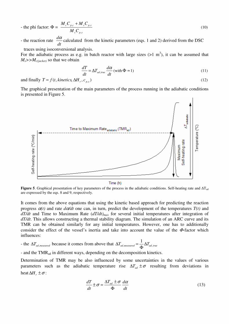
The graphical presentation of the main parameters of the process running in the adiabatic conditions

is presented in Figure 5.

Figure 5. Graphical presentation of key parameters of the process in the adiabatic conditions. Self-heating rate and ∆Tad

are expressed by the eqs. 8 and 9, respectively.

It comes from the above equations that using the kinetic based approach for predicting the reaction

progress α(t) and rate dα/dt one can, in turn, predict the development of the temperatures T(t) and

dT/dt and Time to Maximum Rate (dT/dt)max for several initial temperatures after integration of

dT/dt. This allows constructing a thermal stability diagram. The simulation of an ARC curve and its

TMR can be obtained similarly for any initial temperatures. However, one has to additionally

consider the effect of the vessel’s inertia and take into account the value of the Φ-factor which

influences:

- the measuredadT ,∆ because it comes from above that trueadmeasuredad TT ,,

1∆

Φ=∆

- and the TMRad in different ways, depending on the decomposition kinetics.

Determination of TMR may be also influenced by some uncertainties in the values of various

parameters such as the adiabatic temperature rise σ±∆ adT resulting from deviations in

heat σ±∆ rH :

dt

dT

dt

dT ad ασσ

Φ

±∆=± (13)

After all, the numerical integration of dT/dt enables to predict TMR in ISO-ARC tests for several

initial temperatures oT and Φ-factors within some confidence interval.

SIMULATION OF ISO- AND HWS ADIABATIC EXPERIMENTS

In time-consuming adiabatic experiments it seems to be advantageous to use the kinetic

parameters for the prediction of the adiabatic temperature at which the process can be investigated in

a reasonable time scale. Such prediction leads to the optimization of the experimental work because

if an ISO-ARC test is performed at an initial temperature that is too low, then the duration of the

experiment can last over hours or even days. In the current study for a MN mass of 1.5975g and the

ARC bomb with Φ =3.2, taking Cp = 2 J/(g·K) and an average heat release ∆Hr= -2001.7±216.5 J/g

we obtained

dt

dK

dt

d

KgJ

gJ

dt

d

c

H

dt

dT

p

r

αα

α

8.338.123)·/(2

/ 216.52001.7

2.3

1

)(1

±=±

=∆−

Φ=

(14)

The initial temperatures may contain some uncertainties. For an initial temperature CTo °=184

assuming a deviation CTo °±=∆ 1 , after integration one obtains

- a conservative TMR of 4.22 h for =°+= CTo 1184 185°C

and CCTad °=°+=∆ 6.346.8338.123

- a best TMR prediction of c.a. 4.86 hours for CTo °=184 and CTad °=∆ 8.123

- a non-conservative TMR of 5.63 h for =°−= CTo 1184 183°C

and CCTad °=°−=∆ 279 8.338.123

The safety diagram based on these calculations is presented in Figure 6.

Time (h)

8.587.576.565.554.543.53

Tem

pera

ture

(°C

)

194

192

190

188

186

184

182

180

X : 4.86 Y : 184

Figure 6. Thermal safety diagram for 3-methyl-4-nitrophenol simulated for the following parameters:

∆Hr = -2001.7±216.5 J/g, ∆Tad=(-∆Hr)/(CP· Φ) = 312.8±33.8°C, Φ =3.2 and CP = 2 J/g/°C. For an initial ISO-ARC

temperature of 184°C, TMR amounts to ca. 4.86h with the confidence interval (range 4.22-5.63hrs) calculated for the

adiabatic temperatures lower by 1K (top curve) and higher by 1K (bottom curve).

Results shown in Figure 6 illustrate how the kinetic parameters obtained from DSC data enable to

estimate precisely the initial temperature of an ISO-ARC which results in reasonable duration of the

data collection without necessity of carrying out some preliminary HWS testing. However, the ARC

test carried out in a HWS mode can be simulated as well. As presented in Figure 7 (symbols) the

temperature at the detection limit which corresponds usually to a self-heating rate of 0.02 K/min

amounts to ca. 183.8°C with Φ-factor = 3.2 and was reached after 11.29h. The time remaining from

this point to the measured TMR (see Figure 7) amounts to 15.67 – 11.29h = 4.38 h. The measured

TMR value is consistent with the calculated results presented in Figure 6 confirming that an initial

ISO-ARC temperature of 184°C leads to a TMR of about 4.86h. However, some minor reaction

progress α occurs during the initial period of a HWS-ARC test when the sample is still in the heat-

wait-search mode. When the detection limit of the ARC apparatus is reached, the reaction progress α

is no longer = 0, but α > 0. Having the kinetic description of the reaction rate derived from the DSC

data, one can estimate that the reaction progress α after the 11.29 h of HWS testing (Figure 7)

amounts to about 0.0095 (ca. 1%). The simulation of the adiabatic temperature rise from that

temperature of 183.8°C can be further calculated and is presented in Figure 7 as a solid line. The

numerical results are in accordance with the experimental data and indicate that the calculated

remaining TMR is ca. 4.4 h. Presented results show that the good fit of simulated and experimental

results in HWS-ARC test can be additionally applied for the verification of the calculated kinetic

parameters.

Time (h)

1614121086420

Reaction P

rogre

ss (

-)

1

0.8

0.6

0.4

0.2

0

Tem

pera

ture

(°C

)

500

450

400

350

300

250

200

150

100

50 Reaction Progress: 0.0095 (-)

t: 11.29 (h)

T: 183.81 (°C)

t: 15.67 (h)

T: 421.65 (°C(

Figure 7. Typical ARC test for 3-methyl-4-nitrophenol carried out in HWS mode. Having the kinetic description of the

reaction rate from the DSC data, one can estimate that the reaction progress α after ca. 11.3 h of HWS testing amounts to

about 0.0095 (ca. 1%). From the time at which the temperature of the detection limit (183.81°C) was reached the value of

TMR amounts to ca. 4.4h (15.67-11.29h). Solid line depicts the simulation being in a good agreement with the

experimental HWS-ARC data presented as symbols.

The next important advantage of the use of the kinetic parameters derived from DSC data consists in

the possibility of the simulation of the reaction course in fully adiabatic conditions (Φ =1) for the

totally not decomposed sample (α=0) what is very difficult to achieve from the experimental point of

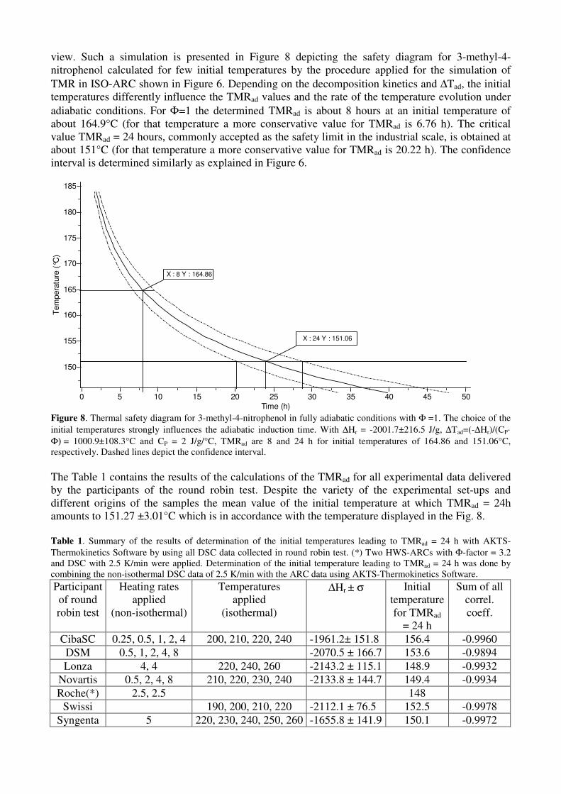
view. Such a simulation is presented in Figure 8 depicting the safety diagram for 3-methyl-4-

nitrophenol calculated for few initial temperatures by the procedure applied for the simulation of

TMR in ISO-ARC shown in Figure 6. Depending on the decomposition kinetics and ∆Tad, the initial

temperatures differently influence the TMRad values and the rate of the temperature evolution under

adiabatic conditions. For Φ=1 the determined TMRad is about 8 hours at an initial temperature of

about 164.9°C (for that temperature a more conservative value for TMRad is 6.76 h). The critical

value TMRad = 24 hours, commonly accepted as the safety limit in the industrial scale, is obtained at

about 151°C (for that temperature a more conservative value for TMRad is 20.22 h). The confidence

interval is determined similarly as explained in Figure 6.

Time (h)

50454035302520151050

Tem

pera

ture

(°C

)

185

180

175

170

165

160

155

150

X : 24 Y : 151.06

X : 8 Y : 164.86

Figure 8. Thermal safety diagram for 3-methyl-4-nitrophenol in fully adiabatic conditions with Φ =1. The choice of the

initial temperatures strongly influences the adiabatic induction time. With ∆Hr = -2001.7±216.5 J/g, ∆Tad=(-∆Hr)/(CP·

Φ) = 1000.9±108.3°C and CP = 2 J/g/°C, TMRad are 8 and 24 h for initial temperatures of 164.86 and 151.06°C,

respectively. Dashed lines depict the confidence interval.

The Table 1 contains the results of the calculations of the TMRad for all experimental data delivered

by the participants of the round robin test. Despite the variety of the experimental set-ups and

different origins of the samples the mean value of the initial temperature at which TMRad = 24h

amounts to 151.27 ±3.01°C which is in accordance with the temperature displayed in the Fig. 8.

Table 1. Summary of the results of determination of the initial temperatures leading to TMRad = 24 h with AKTS-

Thermokinetics Software by using all DSC data collected in round robin test. (*) Two HWS-ARCs with Φ-factor = 3.2

and DSC with 2.5 K/min were applied. Determination of the initial temperature leading to TMRad = 24 h was done by

combining the non-isothermal DSC data of 2.5 K/min with the ARC data using AKTS-Thermokinetics Software.

Participant

of round

robin test

Heating rates

applied

(non-isothermal)

Temperatures

applied

(isothermal)

∆Hr ± σ

Initial

temperature

for TMRad

= 24 h

Sum of all

correl.

coeff.

CibaSC 0.25, 0.5, 1, 2, 4 200, 210, 220, 240 -1961.2± 151.8 156.4 -0.9960

DSM 0.5, 1, 2, 4, 8 -2070.5 ± 166.7 153.6 -0.9894

Lonza 4, 4 220, 240, 260 -2143.2 ± 115.1 148.9 -0.9932

Novartis 0.5, 2, 4, 8 210, 220, 230, 240 -2133.8 ± 144.7 149.4 -0.9934

Roche(*) 2.5, 2.5 148

Swissi 190, 200, 210, 220 -2112.1 ± 76.5 152.5 -0.9978

Syngenta 5 220, 230, 240, 250, 260 -1655.8 ± 141.9 150.1 -0.9972

The TMRad values calculated by the presented method are less conservative as those derived by

using the estimation of Keller et al. (18). He presented the estimation method for TMRad from non-

isothermal DSC measurements based on the model of zeroth order reaction. Similar approach was

presented in the paper of Pastre at al. (19) which verified his model by Dewar vessel experiments.

They proposed the linear regression procedure to find out a conservative value of the initial

temperature that leads to TMRad = 24h as a function of TOnset:

TMRad, 24h (K) = 0.65· TOnset (K)+50 K (15)

If one estimates roughly from Figure 1 that the possible detected onset lays between 220 and 250°C,

then according the Keller’s approximation TMRad = 24h will be reached for initial temperatures

between 97 and 117°C. These values are 30-50°C more conservative compared to presented by us

value of 151°C. Nevertheless, this of Keller’s rule of thumb can be considered as an interesting

preliminary step in a thermal hazard assessment for determining TMRad = 24h .

Influence of ΦΦΦΦ-factor on the reaction course

The interesting feature of the simulation method presented in this paper is the possibility of

the comparison of the predicted signals in isothermal, pseudo-adiabatic and fully adiabatic

conditions.

Time (day)

32.752.52.2521.751.51.2510.750.50.250

Tem

pera

ture

(°C

)

1200

1000

800

600

400

200

0

Reaction P

rogre

ss (

-)1

0.8

0.6

0.4

0.2

0

Φ

151.06°C

Φ

Φ

Φ

Φ

=1

=3.2

=1E10

=1E10

=3.2=1

Φ =3.2HWS-ARC

Φ

Figure 9. Comparison between the T-t relationship (top) and reaction progress (bottom) in isothermal (T=151.06°C) and

adiabatic conditions. TMRad were calculated for a starting temperature of 151.06°C with Φ =3.2 and 1, respectively using

the values of ∆Hr = -2001.7±216.5 J/g and Cp = 2 J/g/°C. Under isothermal conditions the reaction progress α after ca 2.4

days amounts to only ca. 0.038 (3.8%). The decrease of the Φ−factor results in significant shortening of the time required

for the total decomposition which occurs after 2.5 and 1 day for Φ factors 3.2 and 1.0, respectively.

At a constant temperature of 151°C one can see (Fig.9) that the reaction progress α after 3 days

amounts to about 0.038 (ca. 3.8%) only. The decrease of the Φ value significantly changes the time

required for the total decomposition. As presented in this figure the total decomposition under fully

adiabatic conditions occurs after 1 day (24 h) however, with Φ=3.2 (value applied with ARC

calorimeter Fig. 6) the reaction ends after ca. 2.4 days.

Note that isothermal conditions can be numerically retrieved by setting an exceptionally large value

of the thermal inertia factor such as Φ = 1010

to achieve an insignificant adiabatic temperature rise

∆Tad ≈0. If the Φ is very high all heat released by the reaction is dissipated to the surrounding. As a

consequence, the sample temperature remains constant because with

dt

dT

dt

dTtruead

α,

1∆

Φ= (16)

for very large values of Φ we have

0≅dt

dTs and isothermalss TTT ≅=≅= )1()0( αα (17)

Simulated can be not only the temperature but the rate of the heat evolution during self-heating

process as well. The simulated reaction rate in fully adiabatic conditions (Φ=1) as a function of

temperature (top) and time (bottom) is presented in Figure 10.

Temperature (°C)

11001000900800700600500400300200

Self-h

eating r

ate

(°C

/min

)

1.00E-3

1.00E-2

1.00E-1

1.00E+0

1.00E+1

1.00E+2

1.00E+3

1.00E+4

1.00E+5

1.00E+6

1.00E+7

Time (h)

2522.52017.51512.5107.552.50

Self-h

eating r

ate

(°C

/min

)

1.00E-3

1.00E-2

1.00E-1

1.00E+0

1.00E+1

1.00E+2

1.00E+3

1.00E+4

1.00E+5

1.00E+6

1.00E+7

1.00E+8

Time: 13.8 (h)

Temperature: 160.6 (°C)

Self-heating rate: 0.02 (°C/min)

Reaction progress: 0.0095

Figure 10. Simulated self-heating rate curves for 3-methyl-4-nitrophenol under adiabatic conditions (Φ=1) as a function

of temperature (top) and time (bottom) calculated for an initial temperature of 151°C. Typical detection limit of adiabatic

calorimeters (0.02 K/min) is reached after 13.56 hours i.e. 10.44 hours before TMRad = 24 h. Reaction progress at 13.56 h

amounts to about 0.0095 (ca. 1%).

The simulation indicates that the typical detection limit of the heat evolution rate 0.02 K/min is

reached after 13.8 h i.e. 10.2 h before TMRad value of 24h. During this initial period of the adiabatic

reaction the sample starts to decompose, the reaction progress at the point of the detection limit

amounts to 0.0095 (ca. 1%). Even such a small reaction progress can influence the value of the time

remaining to 24h, this issue is discussed in the following paragraph.

INFLUENCE OF REACTION PROGRESS OCCURRING DURING INITIAL PERIOD OF

HWS ADIABATIC EXPERIMENT ON DETERMINATION OF TMRad

The correct interpretation and simulation of the adiabatic experiments requires introducing

into considerations the problem of the certain, unknown degree of the decomposition of the

investigated material which starts to decompose before the temperature of the detection limit is

reached. This, even being relatively small, reaction progress leads to the shortening TMRad value

comparing to the value characteristic for the absolutely not decomposed material having the reaction

progress α=0.

The simulation of the TMRad for the samples with different initial decomposition degree α (in the

range 0-5%) is depicted in Figure 11. The value of TMRad =24h for the initial temperature of about

151°C and the sample with α=0 decreases to 23.03; 21.49; 17.59 and 9.75h for the samples with the

reaction progress of 0.001, 0.01; 0.025, and 0.05, respectively.

Time (h)

2522.52017.51512.5107.552.50

Tem

pera

ture

(°C

)

1200

1000

800

600

400

200

TMRad = 24h

151.06°C

5% 2.5%1% 0.1% 0%

Figure 11. Influence of preliminary reaction progress α on TMRad values. Note that the reaction progress α is displayed

in percent.

Presented results of the simulations clearly show that a special care has to be taken when interpreting

results of TMRad obtained experimentally for the sample with unknown decomposition degree (like

in HWS-ARC). This uncontrolled reaction progress depends not only on the experimental settings

(the choice of the initial temperature in adiabatic experiments) but also on the kinetics of the

decomposition. Depending on the kind of the rate-controlling step in the decomposition process this

influence of the preliminary α value on the TMRad can be different and this issue will be discussed in

our next paper.

CONCLUSION

The decomposition of 3-methyl-4-nitrophenol samples of different origins was studied using

DSC and ARC. The DSC results delivered by the participants of a round robin test and obtained with

different heating rates (non-isothermal mode) and at different temperatures (isothermal mode) were

elaborated by AKTS-Thermokinetics software and applied for the determination of the kinetic

parameters of the decomposition reaction. Due to their precise determination, the variation of the

runaway time under true adiabatic mode (with a thermal inertia factor Φ = 1) was calculated for any

initial process temperature. Results were reported in a thermal safety diagram depicting the

dependence of Time to Maximum Rate (TMR) on the initial temperature. The critical value

TMRad=24 hours was obtained for the initial adiabatic temperature of about 151°C. Both isothermal

DSC and adiabatic experiments with Φ-factor > 1 were used for the final validation of the kinetic

parameters.

The precise kinetic description of the process allowed simulation of the influence of the Φ-factor

value on the reaction course. Due to the possibility of the simulation of ISO- and HWS modes of the

ARC experiments the applied method can help in the optimal choice of the initial adiabatic

temperature what results in shortening of the time required for the adiabatic investigations. The

knowledge of the kinetic parameters of the reaction allowed determining reaction progress occurring

in the initial period of the adiabatic experiment before reaching by the system the detection limit of

the heat evolution. Presented simulations showed that the influence of this initial reaction progress on

the TMRad value has to be carefully considered because even not significant reaction progress as e.g.

0.025 can decrease by ca. 6.4h the value of TMRad (24h for α=0 and ca. 17.6h for α=0.025).

REFERENCES

1. A.Zogg, F. Stoessel, U. Fischer and K. Hungerbühler, Thermochim. Acta, 2004, 419, 1

2. D.J. am Ende, D.B.H. Ripin and N.P. Weston, Thermochim. Acta, 2004, 419, 83.

3. S.-Y. Liu, J.-M. Tseng, M.-K. Lee and T.-C. Wu, J. Therm. Anal. Cal., 2009, 95, 559.

4. A. Bhattacharya, Chem. Eng. J., 2005, 110, 67.

5. D.I. Towsend and J.C.Tou, Thermochim. Acta, 1980, 37, 1.

6. Y.Iizuka and M. Surianarayanan, Ind. Eng. Chem. Res.,2003, 42, 2987.

7. G.T. Bodman and S. Chevrin, J.Hazard. Materials, 1994, 115, 101.

8. P.F. Bunyan, T.T. Griffiths and V.J. Norris, Thermochim. Acta, 2003, 401, 17.

9. R.J.A. Kersten, M.N. Boers, M.M. Stork and C. Visser, J. Los.Prev. Process. Ind., 2005, 18,

145.

10. B. Roduit, W. Dermaut, A. Lunghi, P. Folly, B. Berger and A. Sarbach, J. Therm. Anal. Cal.,

2008, 93, 163.

11. B. Roduit, P. Folly, B. Berger, J. Mathieu, A. Sarbach, H. Andres, M. Ramin and B.

Vogelsanger, J. Therm. Anal. Cal., 2008, 93, 153.

12. B. Roduit, L. Xia, P. Folly, B. Berger, J. Mathieu, A. Sarbach, H. Andres, M. Ramin, B.

Vogelsanger, D. Spitzer, H. Moulard and D. Dilhan, J. Therm. Anal. Cal., 2008, 93, 143.

13. AKTS-Thermokinetics and AKTS-Thermal Safety software, AKTS AG, Advanced Kinetics

and Technology Solutions, http://www.akts.com.

14. Swiss Institute of Safety and Security, http://www.swissi.ch/index.cfm?rub=1010.

15. H. L. Friedman, J. Polym. Sci, Part C, Polymer Symposium (6PC), 1964, 183.

16. K.H. Schoenborn, Thermochim. Acta, 1993, 69, 103.

17. M.E. Patt, B.E. White, B. Stein and E.J. Cotts, Thermochim. Acta, 1992, 197, 413.

18. A.Keller, D. Stark, H. Fierz, E. Heinzle and K. Hungerbühler, J.Loss.Prev.Ind., 1997, 10, 31.

19. J. Pastre, U.Wörsdörfer, A. Keller and K. Hungerbühler, J.Loss.Prev.Ind., 2000, 13, 7.