Embed Size (px)
Citation preview

Estimation of the Heat and Water Budgets of the Persian (Arabian) GulfUsing a Regional Climate Model*,1
PENGFEI XUE
Great Lakes Research Center, Department of Civil and Environmental Engineering, Michigan Technological University,
Houghton, Michigan
ELFATIH A. B. ELTAHIR
Department of Civil and Environmental Engineering, Massachusetts Institute of Technology, Cambridge, Massachusetts
(Manuscript received 9 March 2014, in final form 9 January 2015)
ABSTRACT
Because of the scarcity of observational data, existing estimates of the heat and water budgets of the Persian
Gulf are rather uncertain. This uncertainty leaves open the fundamental question ofwhether this water body is a
net heat source or a net heat sink to the atmosphere. Previous regional modeling studies either used specified
surface fluxes to simulate the hydrodynamics of the Gulf or prescribed SST in simulating the regional atmo-
spheric climate; neither of these two approaches is suitable for addressing the above question or for projecting
the future climate in this region. For the first time, a high-resolution, two-way, coupled Gulf–atmosphere re-
gional model (GARM) is developed, forced by solar radiation and constrained by observed lateral boundary
conditions, suited for the study of current and future climates of the PersianGulf. Here, this study demonstrates
the unique capability of this model in consistently predicting surface heat and water fluxes and lateral heat and
water exchanges with theArabian Sea, as well as the variability of water temperature andwatermass. Although
these variables are strongly coupled, only SST has been directly and sufficiently observed. The coupled model
succeeds in simulating the water and heat budgets of the Persian Gulf without any artificial flux adjustment, as
demonstrated in the close agreement of model simulation with satellite and in situ observations.
The coupled regional climate model simulates a net surface heat flux of 13Wm22, suggesting a small net
heat flux from the atmosphere into the Persian Gulf. The annual evaporation from the Persian Gulf is
1.84m yr21, and the annual influx and outflux of water through the Strait of Hormuz between the PersianGulf
and Arabian Sea are equivalent to Persian Gulf–averaged precipitation and evaporation rates of 33.7 and
32.1m yr21, with a net influx of water equivalent to a Persian Gulf–averaged precipitation rate of 1.6m yr21.
The average depth of the Persian Gulf water is;38m. Hence, it suggests that the mean residency time scale
for the entire Persian Gulf is ;14 months.
1. Introduction
The Persian (Arabian) Gulf (hereafter referred to as
the Gulf) is a semienclosed shallow sea between Iran
(Persia) and the Arabian Peninsula, connected with the
Gulf of Oman and the Indian Ocean through the Strait
of Hormuz (hereafter referred to as the Strait). From the
Strait, the Gulf stretches northwest for about 1000km to
Shatt al Arab (Arvand Roud) with a width that varies
from a maximum of ;340 km to a minimum of ;55km
at the Strait. The water depth in the Gulf ranges from a
few meters near the coast to more than 100m at the
Strait, with a mean depth of ;38m (Fig. 1a). The pri-
mary circulation pattern is a cyclonic gyre with the in-
flow of Arabian Sea waters coming mainly through the
northern part of the Strait and forming a cyclonic cir-
culation gyre returning to the southern Gulf (Reynolds
1993). The northern Gulf can maintain a smaller cy-
clonic circulation while southward coastal currents exist
between the head of the Gulf and Qatar and extend to
* Supplemental information related to this paper is available at the
Journals Online website: http://dx.doi.org/10.1175/JCLI-D-14-00189.s1.1Great Lakes Research Center at Michigan Technological
University Contribution Number 19.
Corresponding author address: Dr. Pengfei Xue, Michigan
Technological University, 1400 TownsendDr., BuildingGLRC-317,
Houghton, MI 49931.
E-mail: [email protected]
1 JULY 2015 XUE AND ELTAH IR 5041
DOI: 10.1175/JCLI-D-14-00189.1
� 2015 American Meteorological Society

the east of Qatar and north of United Arab Emirates
(UAE) with an outflow through the southern part of the
Strait (Fig. 1b).
Surrounded by natural geologic formations that
contain two-thirds of the world’s estimated proven oil
reserves and one-third of the world’s estimated proven
natural gas reserves, the Gulf is located in an important
economic and political region, representing the most
important route for global transport of oil and gas. The
countries surrounding the Gulf are experiencing some
of the highest rates of economic and population
growths, resulting in an increasing level of environ-
mental stress (Sheppard et al. 2010). More than any
other water body, the Gulf water is desalinated at an
increasing rate to provide the main source of water
supply for most of the population in the surrounding
cities and countries. The surface water temperature in
the Gulf has also exhibited a significant increase in the
recent two decades (Shirvani et al. 2014). Concerns are
rising about sustainability of these trends into the fu-
ture, while climate change and its impacts complicate
this situation even further (Hamza and Munawar 2009;
Sale et al. 2011).
Because of the limited observational data, previous
estimates of heat and water budgets are highly un-
certain. This is a major hurdle in understanding the
current climate of the Gulf system and in projecting
its future trends. The annual-mean value of net
FIG. 1. (top) The geographic features and (bottom) the schematic of the circulation of the
Gulf shown with grey-brown arrows. Air–sea interactions are indicated by red-brown arrows.
The color of the Gulf indicates the water depth (warmer color for deeper water).
5042 JOURNAL OF CL IMATE VOLUME 28

surface heat flux estimated by various studies ranges
from 166Wm22 flux into the Gulf to 221Wm22 loss
from the Gulf (Ahmad and Sultan 1991; Hastenrath
et al. 1979; Johns et al. 2003; Prasad et al. 2001;
Abualnaja 2009). [The net surface heat flux is the bal-
ance between incoming solar radiation, reflected
solar radiation, downward longwave radiation, upward
longwave radiation, latent heat flux (evaporation), and
sensible heat flux.] This uncertainty leaves open the
fundamental question of whether this water body is a net
heat source or a net heat sink to the atmosphere. Our
knowledge of the rate of evaporation, which is a signif-
icant component of both the heat budget and water
budget, has also been quite uncertain, with estimates
ranging from 1.4 to 2.1myr21 (Privett 1959; Meshal and
Hassan 1986; Hastenrath et al. 1979; Ahmad and Sultan
1991; Johns et al. 2003). A summary of the previous
estimates of the surface heat flux and evaporation rate is
presented in Table 1.
To characterize the heat and water budgets of the
Gulf, we need to constrain consistent estimates of
evaporation, net surface heat flux, and lateral heat flux.
The dominance of the fluxes in regulating SST is due to
the shallow nature and semienclosed basin of the Gulf.
Given the shallow nature of this water body (average
depth of 38m), the SST is as much a reflection of these
surface fluxes as a forcing of the fluxes. In water bodies
that are as shallow as the Gulf, the water mixed layer
and atmospheric mixed layer are of comparable heat
content, and the two components of a coupled system
evolve simultaneously with significant two-way in-
teractions. Previous regional modeling studies either
used specified surface fluxes to simulate the hydrody-
namics of the Gulf (Chao et al. 1992; Kämpf and
Sadrinasab 2006; Sadrinasab and Kämpf 2004; Thoppil
and Hogan 2010; Yao and Johns 2010a; Yao and Johns
2010b; Hassanzadeh et al. 2011; Hassanzadeh et al.
2012) or prescribed SST in simulating the regional at-
mospheric climate (Evans et al. 2004; Marcella and
Eltahir 2008, 2012). Because of the shallow nature of
this water body, neither of these two approaches is
suitable for addressing the above questions or
projecting future climate in this region. The most
suitable approach is to consistently estimate evap-
oration and all other heat fluxes through the use of a
laterally constrained and vertically coupled Gulf–
atmosphere model.
The remaining part of this paper is organized as
follows: Section 2 describes the data used in this study,
the coupled ocean–atmosphere model, and the design
of experiments. Section 3 presents the results of the
coupled simulation in comparison to uncoupled sim-
ulations and observational data. In section 4, the heat
and water budgets are examined at both seasonal and
annual time scales. The discussion is presented in
section 5, and brief conclusions are summarized in
section 6.
2. Methods
a. Model
To the best of our knowledge, this is the first cou-
pled ocean–atmosphere model developed for the
Gulf, known as the Gulf–atmosphere regional model
(GARM), in which we synchronously coupled a re-
gional ocean model to a regional atmospheric climate
model. The Gulf model was developed using un-
structured grid Finite Volume Coastal Ocean Model
(FVCOM) (Chen et al. 2003). With the merit of an
unstructured grid for ideal geometrical fitting (Chen
et al. 2006; Tian and Chen 2006; Xue et al. 2009),
FVCOM has gained its popularity in research and
applications to estuaries and coastal oceans (Weisberg
and Zheng 2006; Chen et al. 2008; Cowles et al. 2008;
Zhao et al. 2010; Xue et al. 2011; Beardsley et al. 2013;
Chen et al. 2014). The horizontal resolution of the
model grid varies from;3 km near the coast to;5 km
in the offshore region of the Gulf and gradually de-
creases to 10–15 km close to the open boundary
(Fig. 2). As the Gulf is a shallow-water system with a
mean depth of ;38m, the model is configured with 30
generalized sigma layers, in which 30 uniform sigma
layers are configured to provide the vertical resolution
of ,1m for nearshore waters and ;(1–2) m in most
offshore regions of the Gulf. Climatological monthly
mean fields of temperature (Locarnini 2010) and sa-
linity (Antonov 2010) from the World Ocean Atlas
2009 (WOA09), which consists of 18 objectively ana-
lyzed, climatological fields of in situ temperature and
TABLE 1. Basin-averaged annual-mean heat fluxes and evapo-
ration rate of the Gulf, estimated by previous studies. N/A means
not applicable.
References
Net
(Wm22)
Latent
(Wm22)
Evaporation
(m yr21)
Privett (1959) N/A 114.16 1.44
Hastenrath et al. (1979) 45 110.00 1.39
Meshal andHassan (1986) N/A 160.13 2.02
Ahmad and Sultan (1991) 221 168.00 2.12
Prasad et al. (2001) 66 N/A N/A
51 N/A N/A
63 N/A N/A
Johns et al. (2003) 27 6 4 145.07 1.83
4 122.00 1.58
Abualnaja (2009) 8 N/A N/A
1 JULY 2015 XUE AND ELTAH IR 5043

salinity at standard depth levels for annual, seasonal,
and monthly compositing periods for the World
Ocean, are applied to the model open boundary. The
mean flow velocity boundary condition is dynamically
calculated in the model based on the wind and water
temperature and salinity information to resolve the
wind-driven and buoyancy-driven mean flow compo-
nents. The major freshwater inflow from the Shatt al
Arab (Arvand Roud) formed by the confluence of the
Euphrates, Tigris, and Karun Rivers was specified
based on the streamflow statistics for the Tigris River
and Euphrates River basins (Saleh 2010). The clima-
tological monthly mean of the river inflow is used with
an annual-mean transport of 1576m3 s21 and high-
flow seasons between March and May (Table 3). The
surface forcing (surface wind, precipitation, evapora-
tion, shortwave and longwave radiation, and latent
and sensible heat fluxes) is provided by the atmo-
spheric model at 3-h intervals. The Mellor–Yamada
level-2.5 turbulence closure (Mellor and Yamada
1982) scheme is used for vertical mixing parameteri-
zation, and the horizontal diffusion is parameterized
using Smagorinsky formulation (Smagorinsky 1963).
The external and internal mode time steps are 6.0 and
60.0 s, respectively.
The atmospheric model, the Massachusetts Institute
of Technology (MIT) regional climate model
(MRCM), is an advanced version of the Regional Cli-
mate Model, version 3 (RegCM3) (Giorgi and Mearns
1999; Pal et al. 2007), with a focus on improving the skill
of RegCM3 in simulating climate over different regions
through the incorporation of new physical schemes or
modification of original schemes, including coupling of
the Integrated Biosphere Simulator (IBIS) land surface
scheme (Winter et al. 2009), new convective cloud
scheme (Gianotti and Eltahir 2014a), new convective
rainfall autoconversion scheme (Gianotti and Eltahir
2014b), modified boundary layer height and boundary
layer cloud scheme (Gianotti 2013), and new surface
albedo assignment (Marcella and Eltahir 2012) and
irrigation scheme (Marcella and Eltahir 2014). Ocean
surface fluxes in MRCM are handled by Zeng’s bulk
aerodynamic ocean flux parameterization scheme
(Zeng et al. 1998) with SST fields provided by the ocean
model in the coupled simulation. Owing to the different
spatial scales of atmospheric and Gulf circulation, the
FIG. 2. The unstructured triangular mesh of the Gulf model.
5044 JOURNAL OF CL IMATE VOLUME 28

MRCM is configured to cover a larger domain between
128 and 40.58N and 298 and 618E with 30-km resolution
in 120 3 120 grids.
Since our long-term research goal is to project the
impact of future climate on the Gulf and only global
general circulationmodels may provide the atmospheric
model boundary conditions for the future climate, we
chose datasets that describe the current climate (1981–
90) as simulated by the ECHAM51/Max Planck Institute
Ocean Model (MPIOM) climate model of the Max
Planck Institute for Meteorology, which has now been
updated and renamed the Max Planck Institute Earth
System Model (MPI-ESM) in the phase 5 of the Cou-
pled Model Intercomparison Project (CMIP5), to pro-
vide atmospheric boundary conditions to our regional
model in this study. Considered one of the better global
climate models, its skill has been documented in a spe-
cial issue of the Journal of Climate (2006, Vol. 19, No.
16) devoted to climate models at the Max Planck In-
stitute for Meteorology. The initial and boundary con-
ditions were specified at 6-h intervals [in a sensitivity
analysis, a second coupled simulation driven by ERA-40
reanalysis datasets has also been conducted and the re-
sults are quite similar to those using ECHAM5 (see
section 5)]. The lateral boundary condition includes the
surface pressure and wind components, air temperature,
vertical velocity, relative humidity, and geopotential
height at all vertical sigma levels.
While the atmosphere-only MRCM simulation uses
prescribed SST (obtained from ECHAM5/MPIOM
dataset) as the surface boundary condition, the SST in-
formation in the coupled model simulation is predicted
by the Gulf–FVCOM model and provided to the
atmospheric–MRCM model. The MRCM runs with a
time step of 60 s, and the radiation scheme and land
surface scheme are run every 30min and every 180 s,
respectively. The FVCOM and MRCM are coupled
using the Ocean Atmosphere Sea Ice Soil coupler, ver-
sion 3 (OASIS3), software in parallelized computation
environment (Valcke 2013).
To assess the significance of two-way air–sea feed-
back processes in shaping the climate of the Gulf,
uncoupled model experiments were also carried out.
The atmosphere-only simulation with the MRCM,
forced with SST from the ECHAM/MPIOM database,
was conducted to estimate the atmospheric surface
forcing, which was then used to drive an ocean-only
model (FVCOM) simulation. The design of the ex-
periments performed in this study is summarized in
Table 2.
b. Data
For the comparison of the SSTs from the coupled and
ocean-only model simulations, we use two datasets for
verification: NOAA optimum interpolation daily SST
analysis 0.258 3 0.258 resolution gridded data (Reynolds
et al. 2007) (OISST only available from 1982) and
Simple Ocean Data Assimilation (SODA 2.2.4) with
0.58 3 0.58 resolution gridded data (Carton and Giese
2008), selected for the simulation years 1981–90.
3. Model data comparison
Figure 3 presents the Gulf-averaged SST2 simulated
with the coupled and uncoupled ocean-only models for
1980s. Results of the coupled model simulation
demonstrate a close agreement with the observed
OISST and the SODA-assimilated product, successfully
reproducing both an equilibrium mean state of ;268Cand the large seasonal variability of ;14.58C. In con-
trast, the SST of the uncoupled simulation shows a cold
drift for the first 2 yr and reaches a significantly colder
equilibrium state (Fig. 3). The coupledmodel simulation
also demonstrates significant skills in reproducing a
general spatial pattern of the SST with larger variation
in the northwest coast and smaller in the southeast near
the Strait (Fig. 4). During wintertime, the averaged SST
is between 168 and 208C with colder waters occupying
the northwest of the Gulf and relatively warmer waters
in the southeast of the Gulf. During summertime, the
warm surface water of ;318C occupies the entire Gulf
with weaker spatial gradients of SST between 308 and
TABLE 2. Experimental design of coupled and uncoupled model
simulations.
Experiment design SST
Lateral boundary
(atmosphere/ocean)
Coupled model (case 1) Simulated ECHAM5/WOA09
Coupled model (case 2) Simulated ERA-40/WOA09
Atmosphere-only model Prescribed ECHAM5/WOA09
Ocean-only model Simulated N/A/WOA09
1 ECHAM is the global climate model, created by modifying the
global forecast models developed by the European Centre for
Medium-Range Weather Forecasts (ECMWF). The model was
given its name as a combination of its origin (the EC being short for
ECMWF) and the place of development of its parameterization
package, Hamburg.
2 To make the comparisons consistent, SODA and OISST
datasets are first interpolated into FVCOM model grids and then
the Gulf-averaged SST are calculated as grid size–weighted aver-
age based on the area of individual control volume (CV) also called
the tracer control element (TCE) associated with each FVCOM
model grid.
1 JULY 2015 XUE AND ELTAH IR 5045

328C. The uncoupled model simulation, on the other
hand, shows a systematic cold bias over the entire basin
in all seasons.
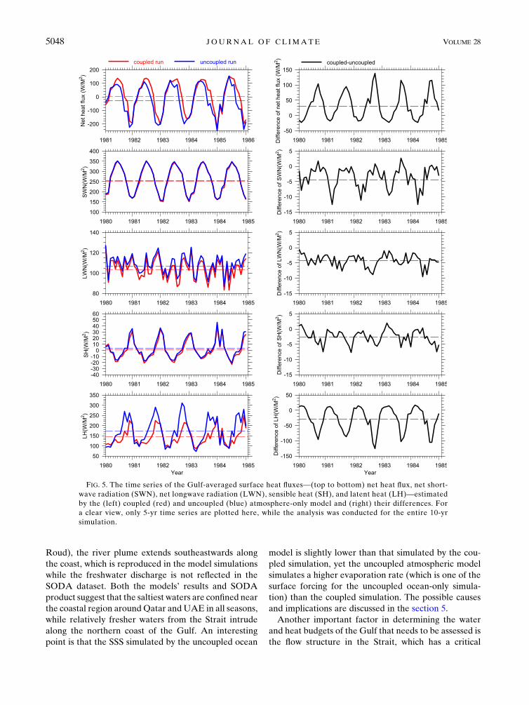
Consistent with the large difference in the simulated
SSTs between the coupled and uncoupled (ocean only)
model simulations, significant differences in the esti-
mated surface heat fluxes are found between the cou-
pled and uncoupled (atmosphere only) model
simulations (Fig. 5, top panels). Estimated from the
simulation with the atmosphere-only model, the net
surface heat flux prescribed to force the uncoupled
ocean model has a decadal-averaged mean value of
;227Wm22. This prescribed value indicates a net heat
loss from the Gulf to the atmosphere, while the coupled
modeling system estimates a net surface heat flux of
;13Wm22, suggesting a small net heat flux from the
atmosphere into the Gulf. The 30Wm22 difference is
clearly responsible for the cold bias of the uncoupled
simulation. Moreover, the net surface heat flux simu-
lated by the uncoupled model also shows a phase shift of
the seasonal cycle, resulting in an oscillation pattern
when comparing the difference in the net surface heat
flux simulated by the uncoupled and coupled model
(Fig. 5, top-right panel); such a phase shift is also re-
flected in the SST simulations in Fig. 3.
A close examination of each component of the surface
heat fluxes in the coupled and uncoupled simulations
reveals that the largest difference in the surface heat
budget comes from the latent heat flux, not surprisingly,
because of the excessive evaporation in the Gulf (Fig. 5,
middle and bottom panels). The atmosphere-onlymodel
overestimates the latent heat loss from the Gulf by
27Wm22, which accounts for ;90% of the total dis-
crepancy between the net surface heat flux estimated by
the atmosphere-only model and by the coupled model.
The differences in other heat flux components estimated
by atmosphere-only and coupled simulations are at least
one order of magnitude smaller than the difference in
latent heat flux and only account for ;10% of the total
difference in the surface heat budget. The atmosphere-
only model and coupled model estimate annual-mean
values of latent heat flux of 173 and 146Wm22.Assuming
the latent heat of vaporization Le 5 2.5 3 106 Jkg21,
corresponding surface evaporation rates are 2.2 and
1.84myr21, respectively. The former is close to the up-
per end (Ahmad and Sultan 1991) of a wide range of
estimates of evaporation by previous observation-based
studies, while the latter is closer to the ensemblemean of
these studies (Table 1; Privett 1959; Meshal and Hassan
1986; Hastenrath et al. 1979; Ahmad and Sultan 1991;
Johns et al. 2003). In addition, observations at two in-
dividual sites (Bushehr and Bandar–Abbass) in Iran lo-
cated near the northern coast of the Gulf are documented
with long-term mean values of evaporation rates of 1.57
and 1.61myr21 (Sabziparvar et al. 2011; Sabziparvar et al.
2013) and reasonably agree with the Gulf-averaged esti-
mates of the coupled simulation as well as local estimates
from the closest model grids of 1.75 and 1.82myr21. A
further analysis of the differences in the relative humidity
and wind speed in the coupled and uncoupled simulations
shows that the lower relative humidity and higher wind
speed in the uncoupled simulation accounts for the
FIG. 3. The time evolution of the Gulf-averaged SST using the coupled (green) and uncoupled (red) ocean-only
model compared with two independent SST datasets: daily OISST (aquamarine) and SODA (blue) surface layer
(5m) temperature for the years 1981–90.
5046 JOURNAL OF CL IMATE VOLUME 28

overestimated heat loss (see Figs. S1 and S2 in the sup-
plemental material, available online at http://dx.doi.org/
10.1175/JCLI-D-14-00189.s1.).
As an evaporation-driven system, the freshwater loss
through the surface evaporation plays an import role in
the formation of the high-salinity water body in theGulf.
Therefore, the model performance in the simulation of
salinity should be an additional evidence of the accuracy
of the model. Figure 6 presents the comparison of
sea surface salinity (SSS) estimated from the SODA
dataset, the coupled model, and the uncoupled ocean
model. Both model simulations and SODA data show a
good agreement of the horizontal distribution of the
SSS. Water with salinity between 40 and 41 occupies
most of the Gulf region except near the Strait with
highly saline water (salinity . 41) existing in the
southern Gulf. During the springtime with a large
amount of freshwater from the Shatt al Arab (Arvand
FIG. 4. Horizontal distributions of decadal-averaged SST in (left) February (coldest month) and (right) August
(warmest month) from (top to bottom) OISST and the coupled and uncoupled model simulations. The numbers in
the panels represent the temperature that corresponds with its color scale value.
1 JULY 2015 XUE AND ELTAH IR 5047
Roud), the river plume extends southeastwards along
the coast, which is reproduced in the model simulations
while the freshwater discharge is not reflected in the
SODA dataset. Both the models’ results and SODA
product suggest that the saltiest waters are confined near
the coastal region aroundQatar andUAE in all seasons,
while relatively fresher waters from the Strait intrude
along the northern coast of the Gulf. An interesting
point is that the SSS simulated by the uncoupled ocean
model is slightly lower than that simulated by the cou-
pled simulation, yet the uncoupled atmospheric model
simulates a higher evaporation rate (which is one of the
surface forcing for the uncoupled ocean-only simula-
tion) than the coupled simulation. The possible causes
and implications are discussed in the section 5.
Another important factor in determining the water
and heat budgets of the Gulf that needs to be assessed is
the flow structure in the Strait, which has a critical
FIG. 5. The time series of the Gulf-averaged surface heat fluxes—(top to bottom) net heat flux, net short-
wave radiation (SWN), net longwave radiation (LWN), sensible heat (SH), and latent heat (LH)—estimated
by the (left) coupled (red) and uncoupled (blue) atmosphere-only model and (right) their differences. For
a clear view, only 5-yr time series are plotted here, while the analysis was conducted for the entire 10-yr
simulation.
5048 JOURNAL OF CL IMATE VOLUME 28

FIG. 6. Horizontal distributions of decadal-averaged surface layer salinity in (top to bottom) February, May, August, and November from
(left to right) the SODA dataset and coupled and uncoupled model simulations.
1 JULY 2015 XUE AND ELTAH IR 5049

impact on lateral transport of both water and heat
through the Strait. As hydrographical samplings were
hardly available in the Strait, we chose to make a com-
parison of simulated flow structure with one of the re-
cently published observations near the Strait by Johns
et al. (2003). We note here that the section covered by
observations is from one of their cruises made in March
1997 across the southern half of the Strait, while our
climate model simulation was performed for the 1980s.
Yet, the model-simulated monthly climatology of inflow
and outflow structures in March is still quite similar to
the observations (Fig. 7). Both observational data and
model simulation show a primary deep-water outflow at
the southern side of the transect,;10km away from the
Oman coast; a primary inflow located in the northern
side of the transect as well as very weak surface inflow
near the Oman coast. [The observation clearly identified
the edge of the inflow core but was not able to sample
farther north. According to Johns et al. (2003), their
research clearances were only available fromOman and
therefore the northern half of the Strait in Iran’s terri-
torial waters could not be sampled.] It would not be
accurate to make direct comparison between a cruise
sampling and model-simulated climatological monthly
mean flow, and hence we estimated the variability of the
inflow and outflow in March using the climatological
daily mean values from the model simulation, which
have standard deviations of 0.15 and 0.1m s21 with
maximum values of 0.65 and 0.5m s21, respectively. The
large variability (the variability of instantaneous flow
shall be even larger) implies that the differences be-
tween the simulated mean flow and observed in-
stantaneous flow are in a reasonable range. More
importantly, only one long-term velocity measurement
FIG. 7. (top left) Cross-section mean flow velocity and the (top right) location of the sampling transect (dot within outlined rectangle),
observational data reproduced from the Johns et al. (2003) cruise sampling inMarch 1997. (bottom) The simulated climatological monthly
cross-section velocity in March from the coupled simulation. The velocities in the panels are in cm s21.
5050 JOURNAL OF CL IMATE VOLUME 28

(Johns et al. 2003) from the ADCP at the southern side
of this transect at 80-m depth shows that the 15-day low-
pass filteredmean flow ranges from0.2 to 0.3ms21, which
is in a very good agreement with the model-simulated,
climatological, monthly mean velocity (0.3m s21) at the
transect.
4. Water and heat budgets
a. Formulation of water and heat balance
The water balance in the Gulf is controlled by 1) lat-
eral water exchange with the Arabian Sea through the
Strait including inflow and outflow and 2) water fluxes in
and out of the Gulf through rainfall, river flow, and
evaporation. This balance is formulated as
dV
dT5P2E1R1Lin 2Lout , (1)
where dV is the change in total water volume over
time scale dT. The terms E,P,R,Lin, and Lout are the
water transports by evaporation and precipitation
over the Gulf, the river flow, and the inflow and out-
flow through the Strait. While R is specified, E and P
are calculated by the atmospheric model, and
Lin and Lout are calculated with the currents into and
out of the Gulf through the Strait (vin and vout) in the
ocean model.
The heat balance in the Gulf reflects 1) net surface
heat flux, 2) lateral heat exchange with the Arabian Sea
through the Strait, 3) heat transport associated with
water fluxes in and out of the Gulf (rainfall, river flow,
and evaporation), 4) solar radiation absorbed by the soil
underlying shallow-water regions, and 5) total heat
change in the water body in the Gulf. This total heat
change is the key factor controlling the climate of the
Gulf and surrounding coastal regions. The coupled
model is able to provide a significant insight into the
relative roles of surface heat fluxes and lateral heat
fluxes in controlling the current and future climate of
this system.
The heat balance is given by
dQ
dT5NR2LH2 SH2LTHout1LTHin
2WHE2P 1WHR 2GH, (2)
where dQ is the total heat content change in water
body over the time scale dT, NR is the net radiation
flux over the Gulf, LH and SH are the latent and
sensible heat fluxes, and LTHout and LTHin are the
heat transport through the Strait. The term WHR is
the heat transport through the river flow; WHE2P
represents the heat transport carried by the water
volume that leaves the basin through its surface via
the evaporation minus precipitation (should not be
confused with the latent heat) (Tragou et al. 1999;
Sofianos et al. 2002; Johns et al. 2003). The term GH is
radiation flux absorbed by the soil underlying shallow-
water regions:
dQ5 d
ð ð ðVrCpudV , (3)
NR5
ð ðA(Qdsw 2Qusw 2Qulw 1Qdlw) dA , (4)
LTHin 5
ð ðSrCpu(vin � n) dS , (5)
LTHout 5
ð ðSrCpu(vout � n) dS , (6)
WHR5 rCpuR , (7)
WHE2P 5
ð ðA(El 2Pl)udA , (8)
GH5Qnetk
12
eh/hz 2 1
e2 1
!, h, hz
0, h$ hz
,
8>><>>: (9)
where n is the unit normal vector to the section; S is the
area of the transect of the Strait; and r,Cp, u, and V
are the water density, the specific heat capacity, local
water temperature, and total water volume of the Gulf,
respectively. The termsQdsw,Qusw, Qulw, and Qdlw are
local incoming solar radiation, reflected solar radiation,
upward longwave radiation, and downward longwave
radiation, respectively. The quantities El and Pl are
local evaporation and precipitation rates. The termQnet
is the net surface heat flux, k is the empirical absorption
coefficient (0.98), and hz is the effective depth (5m) for
ground heat absorption.
b. Conversion of water and heat fluxes
To compare relative contributions of different physical
processes, water fluxes are converted into equivalent
precipitation–evaporation rates over the Gulf. The
equivalency between a horizontal water flux Fy in units of
cubic meters per second into the Gulf and a precipitation
rate over the Gulf Pr in units of meters per year is
Pr 5Fy
A3 (86, 4003 365 s yr21) , (10)
where A is the surface area of the Gulf of
2:35253 1011 m2. Similarly, the advective heat fluxes are
1 JULY 2015 XUE AND ELTAH IR 5051

converted into the equivalent surface heat fluxes over
the Gulf Fs in units of watts per square meter by
Fs 5
ð ðrCpu(v � n) dS
A, (11)
where r,Cp, u, v, and n are the seawater density, the
specific heat capacity, water temperature, velocity, and
the unit normal vector to the transect of the Strait
(Fig. 1a), respectively.
c. Estimates of water and heat budgets
The water balance of the Gulf is dominated by the
high rate of evaporation and the flux of water through
the Strait (Table 3). All other fluxes (rainfall, river dis-
charge, and desalination) are at least one order of
magnitude smaller. The rate of evaporation is pro-
portional to the rate of latent heat flux from the sea
surface; therefore, the heat andwater budgets are tightly
coupled in the Gulf. The coupled model simulates an
annual evaporation rate of 1.84myr21 and estimates
that the annual influx and outflux of water through the
Strait are equivalent to Gulf-averaged precipitation and
evaporation rates of 33.7 and 32.1myr21. The average
depth h of the Gulf water is 38m. Hence, we estimate
that the mean residency time scale s for the Gulf water
is about 14 months using the definition s5Ah/Lin; yet,
we recognize that there is a wide range of complex dis-
tribution of residency times in the Gulf (Sadrinasab and
Kämpf 2004). The lateral net flux simulated by the
coupled model is equivalent to a Gulf-averaged pre-
cipitation rate of 1.6myr21. This large net influx of
water from the Arabian Sea compensates for 84% of the
high evaporation rate. The model estimates a rainfall
rate of 0.085myr21, mostly during the winter season
(Table 3); the very limited rainfall rate in the Gulf was
previously estimated between 0.07 (Reynolds 1993) and
0.15m s21 (Johns et al. 2003), making a small contribu-
tion of 4%–8% to the water balance. These estimates by
the coupled model, combined with a prescribed river
discharge into the Gulf equivalent to a Gulf-averaged
precipitation rate of 0.21myr21 (Saad 1978; Reynolds
1993), are consistent with the estimates from the recent
study by Johns et al. (Johns et al. 2003; Hassanzadeh
TABLE 3. Basin-averaged, climatological, monthly water flux for the Gulf, 1981–90, estimated by the Gulf–atmosphere model with
ECHAM5 atmospheric boundary. Units are in m month21.
Month Evaporation Precipitation River Lateral (in) Lateral (out) Net
January 20.1325 0.0083 0.0167 3.3833 23.2892 20.0133
February 20.1308 0.0175 0.0217 3.4708 23.3925 20.0133
March 20.1108 0.01 0.03 3.555 23.5317 20.0475
April 20.1125 0.0025 0.0358 3.5575 23.4425 0.0408
May 20.1375 0.0008 0.0308 3.4233 23.3275 20.01
June 20.1375 0 0.0183 3.3167 23.115 0.0833
July 20.1458 0 0.0108 2.8283 22.675 0.0192
August 20.17 0 0.0083 2.31 22.1283 0.0217
September 20.175 0 0.0075 1.8558 21.7167 20.0275
October 20.19 0.0075 0.0083 1.6158 21.4175 0.0242
November 20.2017 0.0208 0.01 1.835 21.7375 20.0733
December 20.1992 0.015 0.0133 2.5033 22.3383 20.0067
Average 20.1533 0.0067 0.0175 2.805 22.6758 0
TABLE 4. As in Table 3, but for the annual-mean water flux.
Year Evaporation Precipitation River Lateral (in) Lateral (out) Net
1981 21.84 0.12 0.21 30.34 228.90 20.06
1982 21.89 0.04 0.21 31.82 230.26 20.07
1983 21.86 0.12 0.21 34.39 232.84 0.02
1984 21.82 0.07 0.21 33.59 231.79 0.27
1985 21.86 0.07 0.21 35.12 233.78 20.24
1986 21.86 0.04 0.21 31.89 230.50 20.21
1987 21.84 0.02 0.21 34.59 232.68 0.30
1988 21.85 0.17 0.21 35.59 234.23 20.12
1989 21.80 0.03 0.21 36.52 235.11 20.15
1990 21.81 0.15 0.21 32.69 231.01 0.23
Average 21.84 0.08 0.21 33.66 232.11 0.00
5052 JOURNAL OF CL IMATE VOLUME 28

et al. 2012). A detailed estimate of the water budgets at
seasonal and annual time scale is presented in Tables 3
and 4.
The surface heat fluxes are the dominant factors in
shaping the seasonal cycle of the water temperature
(Fig. 8; Table 5). At the seasonal time scale, the heat
balance of the Gulf is dominated by two large vertical
fluxes: net surface radiation NR and latent heat
flux LH. The total water heat content shows a strong
seasonality, which is mainly a reflection of the season-
ality in incoming solar radiation and in the latent heat
flux (proportional to evaporation). While the seasonal
cycle of incoming solar radiation is mainly a reflection
of the orbital geometry describing how the earth ro-
tates around the sun, the seasonal cycle of latent heat
(evaporation) reflects variability in incoming radiation,
temperature, wind, and humidity. The latent heat flux
(evaporation) exhibits a seasonal cycle with aminimum
FIG. 8. The model-simulated climatological monthly heat budgets (Wm22) of SWN, LWN, net radiation
(NR 5 SWN 2 LWN), SH, LH, lateral heat flux of inflow and outflow through the Strait (LTHin and LTHout).
TABLE 5. As in Table 3, but for heat flux. Units are Wm22.
Month Shortwave Longwave Latent Sensible Lateral (in) Lateral (out) WH GH Net
January 173.9 2115.3 2126.4 213.3 121.9 2121.3 23.7 20.1 284.4
February 199.2 2100.5 2124.2 210.0 110.9 2108.1 23.1 20.2 236.1
March 243.5 2100.4 2105.3 1.7 125.7 2124.8 22.5 20.3 37.5
April 290.3 2103.7 2106.8 7.7 125.9 2122.5 22.9 20.4 87.5
May 329.2 2110.2 2130.5 15.4 132.3 2130.4 24.6 20.4 100.7
June 342.7 2113.7 2131.0 16.2 132.5 2131.8 25.6 20.5 108.9
July 332.2 2103.9 2138.6 8.8 122.9 2118.3 27.0 20.5 95.7
August 312.6 2103.9 2161.4 7.0 102.6 294.9 28.5 20.4 52.9
September 285.6 2112.1 2166.4 4.0 79.9 274.0 28.6 20.3 8.0
October 229.9 2109.1 2180.6 22.2 71.3 261.4 28.4 20.2 260.7
November 181.0 2108.0 2191.9 213.7 75.4 269.1 27.5 20.1 2134.2
December 162.2 2111.8 2189.7 228.3 99.4 291.9 26.7 20.1 2166.9
Average 257.0 2107.6 2146.1 20.6 108.4 2104.1 25.8 20.3 0.7
1 JULY 2015 XUE AND ELTAH IR 5053

value in March and April and maximum in November
and December; similar cycles are reported in Yao and
Johns (2010a,b). Here, we use the bulk formula of the
latent heat flux LH to examine possible causes of such a
seasonal cycle:
LH5 raLeCeU(qs2 qa) , (12)
where ra is the air density (;1.2 kgm23); Le is the latent
heat of evaporation (;2.5 3 106 J kg21); Ce is the latent
heat transfer coefficient (;1.35 3 1023); U and qa are
the wind speed and the specific humidity of air; and qs is
the saturated specific humidity over saline seawater. The
bulk formula implies the wind speed and specific hu-
midity difference at the air–sea interface (qs 2 qa) are key
factors that control the latent heat flux (evaporation).
The qs is formulated as
qs 5 0:98qsat(Ts) , (13)
FIG. 9. Gulf-averaged climatological daily mean of (top to bottom) specific humidity
(gwater kg21air ) of air (QA) and the saturated specific humidity over saline seawater (QS), their
difference (QS 2 QA), the daily wind speed, and the estimate of the latent heat flux with the
bulk formula [Eq. (12)] using the above climatological daily mean of wind speed andQS2QA.
5054 JOURNAL OF CL IMATE VOLUME 28

where Ts is the sea surface temperature and qsat is the
saturation specific humidity for purewater atTs. The factor
of 0.98 is an approximation to take into account the re-
duction of vapor pressure caused by a typical ocean salinity
(Fairall et al. 1996), with qsat in a formula in (Buck 1981)
qsat50:622es
Pa2 0:378es, (14)
es 5 [1:00071 (3:463 1026Pa)]
3 6:1121 exp
�17:502Ts
240:971Ts
�, (15)
where Pa is the air pressure. Figure 9 (top) shows
the Gulf-averaged climatologically daily value of
qs,qa, and qs 2 qa. With an arid climate, the terms
qs and qa are small between ;(15–30) and 10–
15 gwater kg21air over the Gulf, respectively. Their dif-
ference exhibits a minimum value in March and
maximum in August. The wind speed (Fig. 9), on the
other hand, shows a seasonal cycle with strong wind
of ;6m s21 during the winter seasons and weaker
wind of ;3m s21 during July to September. Although
this simple analysis would not be sufficient to explain the
nonlinear spatiotemporal variability of the latent heat
flux in the coupled system, it indicates the high latent
heat during November and December is caused by the
combination of strong wind as well as relatively large
humidity gradient. The low latent heat flux during
March andApril is because of the small air–sea humidity
difference. The horizontal distributions of the monthly
climatology of wind and humidity are presented in the
supplemental information in Figs. S3–S5 in the supple-
mental material. Figure 9 (bottom) shows that the latent
heat estimated with the simple bulk formula [Eq. (12)]
using the climatological daily value of qs 2 qa and daily
wind speed (Fig. 9). The results show that the simple
bulk calculation reproduces to some extent the seasonal
pattern (Fig. 8) with the outliers of May and June. For a
coupled nonlinear system, we do not expect that the
dynamics could be fully explained by a simple linear
combination of the domain-averaged daily wind and
humidity gradient. Indeed, Fig. 9, along with other re-
sults, indicates the complexity of the Gulf system, which
can only be resolved with a two-way, coupled, ocean–
atmosphere model.
At the annual time scale, however, the heat balance is
dictated by several small fluxes. The coupled model
simulation suggests that the Gulf receives annual net
surface heat flux from the atmosphere of12.7Wm22 and
lateral heat flux through the Strait equivalent to a surface
heat flux over the Gulf of 4.1Wm22. These two small
fluxes are balanced to a large degree by the heat loss
from the Gulf (equivalent to 25.8Wm22) associated
with the heat content carried by net water loss (i.e.,
WHE2P 2WHR). In addition, the solar radiation pen-
etrates through shallow water in coastal areas resulting
in small but significant absorption by the underlying soil
(0.3Wm22). This estimate is quite uncertain, since we
are not aware of any direct measurements of this flux. A
detailed estimate of the heat budgets at seasonal and
annual time scales is presented in Tables 5 and 6.
5. Discussion
In this study,we constrain ourmodel using atmospheric
boundary conditions from simulations by general circu-
lation model ECHAM5. However, a fair question is how
reliable are our model results since they were constrained
by lateral boundary conditions from a model simulation
rather than by observations directly. To address this
question, we have conducted the same coupled simula-
tion experiments with lateral boundary conditions con-
strained by the ERA-40 reanalysis data. The results in
these two cases agree very well, which gives us confidence
in our estimates of heat and water budgets of the Gulf
(Fig. 10). Detailed estimates of water and heat budgets at
seasonal and annual time scales in the simulation exper-
iments withERA-40 boundary condition are presented in
Tables A1–A4 in the appendix.
TABLE 6. As in Table 3, but for annual-mean heat flux. Units are Wm22.
Year Shortwave Longwave Latent Sensible Lateral (in) Lateral (out) WH GH Net
1981 261.3 2112.0 2145.7 0.1 99.1 295.0 25.5 20.3 1.8
1982 258.5 2109.3 2149.6 1.0 103.7 299.8 25.9 20.3 21.9
1983 255.5 2105.1 2147.2 0.9 111.3 2107.2 25.6 20.3 2.1
1984 255.9 2107.1 2144.2 21.9 107.5 2101.9 25.7 20.3 2.4
1985 257.5 2107.2 2147.5 21.5 112.1 2107.9 25.7 20.3 20.7
1986 260.1 2108.0 2147.7 0.3 103.3 299.8 25.8 20.3 1.7
1987 259.7 2110.2 2145.7 0.0 111.3 2106.6 25.9 20.3 2.1
1988 252.2 2106.5 2146.8 22.8 114.7 2111.4 25.5 20.3 26.5
1989 259.1 2110.1 2142.7 20.5 116.2 2110.7 25.6 20.3 5.2
1990 248.7 2101.7 2143.5 20.9 104.8 2100.2 25.4 20.3 1.4
Average 257.0 2107.6 2146.1 20.6 108.4 2104.1 25.7 20.3 0.7
1 JULY 2015 XUE AND ELTAH IR 5055

The fact that only a coupled Gulf–atmosphere model
succeeded in reproducing the observed SST climatology
and demonstrated significant skill in simulating the heat
budget of the Gulf without any flux adjustments is con-
sistent with the hypothesis of a significant two-way, air–sea
coupled process over the Gulf. Here, we show evidence
for the existence of a strong negative air–sea feedback
process over the Gulf. This feedback process tends to
stabilize the system through a local ‘‘SST–latent heat’’
adjustment: a positive (negative) perturbation of SST
causes an increase (decrease) of the saturation specific
humidity at the sea surface and hence increases (de-
creases) the specific humidity gradient at the air–sea in-
terface, which results in an increase (decrease) of the loss
of latent heat from the Gulf, therefore suppressing the
perturbation of SST. This negative feedback can be clearly
identified in a simple numerical experiment. A perturba-
tion was imposed to the SST by artificially increasing the
water temperature by 18C in the upper 5m, the coupled
system recovered and restored the SSTfield in a very short
FIG. 10. Sensitivity analysis. The comparison of the coupled simulation results when lateral atmospheric boundary
conditions are constrained by ECHAM5 (blue) and ERA-40 (red). (a) Decadal-averaged monthly net surface heat
flux over theGulf. (b) Decadal-averagedmonthly lateral heat transport through the Strait (converted into equivalent
surface heat flux over the Gulf). (c) Decadal-averaged monthly evaporation 2 precipitation over the Gulf.
5056 JOURNAL OF CL IMATE VOLUME 28

e-folding time scale of;12h (Fig. 11). The adjustment of
latent heat flux responds with a peak value of;30Wm22
immediately after the SST perturbation, and the magni-
tude of latent heat flux adjustment decreases over time as
the SST is restored toward its equilibrium state. There-
fore, the ability of the coupled model to simulate this
negative feedback process, which allows SST and surface
heat flux to directly interact with each other, is the main
factor thatmade it possible to achieve consistent estimates
of the heat budget and SST over theGulf and advance our
understanding of this system.
It should be pointed out that evaporative cooling is not
necessarily the only mechanism responsible for local neg-
ative air–sea feedbacks, depending on characteristics of a
FIG. 11. The responses of the coupled system to the SST perturbation. (top) Restoration of the SST over the Gulf
after its perturbation driven by the negative feedback process. (middle) As in the top, but zoomed-in to a 5-day time
window. (bottom) Changes in latent heat in response to the SST perturbation.
1 JULY 2015 XUE AND ELTAH IR 5057

coupled system. Xue et al. (2014) discussed negative
feedback mechanisms in the tropical Maritime Continent,
where the evaporative cooling and low-level cloud feed-
back both play dominant roles in controlling the local-
scale, negative, air–sea feedback process. The contribution
of cloud feedback to the adjustment of the surface heat flux
is negligible in the Gulf, as the cloud cover is very limited
and evaporation is so strong in the Gulf. In the SST per-
turbation experiment, the incoming solar radiation
remains nearly unchanged because of the extremely low
coverage of clouds. This is significantly different from
the case in the humid tropical region with intensive con-
vection, where the increased inputs of heat and moisture
into the lower atmosphere increase the formation of low-
level clouds, which act as a shield preventing incoming
solar radiation from reaching the sea surface and accounts
for up to;40%of the total adjustment of surface heat flux
(Xue et al. 2014). In addition, the adjustments of sensible
FIG. 12. Time series of the Gulf-averaged ECHAM5/MPIOM SST (blue) used in the uncoupled, atmosphere-only
model, compared to the OISST (green, available from 1982). Notice a significant overestimation in ECHAM5/
MPIOM SST during the warm seasons, particularly in the first 5 yr.
FIG. 13. The time evolution of the Gulf-averaged SST. The uncoupled atmosphere-only simulation was rerun with the
adjusted SST to generate surfacemeteorological fields, whichwere then used to drive the uncoupled oceanmodel to simulate
SST (blue), in comparison with the original uncoupled simulation (red) and coupled simulation (green) as shown in Fig. 3.
5058 JOURNAL OF CL IMATE VOLUME 28

heat (2.2Wm22) and upward longwave radiation
(1.5Wm22) in response to SST perturbation are also one
order of magnitude smaller than the adjustment of latent
heat due to the strong evaporation and a low Bowen ratio
in the Gulf. This is again regional climate dependent; an-
other example is theLaurentianGreat Lakes regionwhere
the latent heat and sensible heat play comparably impor-
tant roles in controlling the net surface heat flux in the fall
seasons, yet both are negligible during summertime.
Furthermore, as the SST is as much a reflection of the
surface flux as being a forcing of the flux in a shallow-
water system, the high-frequency variability of the SST
must be resolved (using a coupledmodel) to be consistent
with the response time scale of the local air–sea feedback
process, otherwise systematic biases may occur (Xue
et al. 2014). This suggests that a prescription of the
monthly or weekly mean state of SST is inadequate to
resolve the strongly coupled Gulf system. To test this
hypothesis, first we conducted a retrospective analysis for
the prescribed SST used in the atmosphere-only model,
which shows a significantly overestimated temperature
than the observed OISST during the warm (high tem-
perature) seasons, particularly in the first 5 yr (Fig. 12).
This indicates that overestimated SSTs specified in the
uncoupled, atmosphere-only model can result in over-
estimates of the latent heat flux and therefore the net
surface heat loss from the Gulf. Second, we made a cor-
rection to the prescribed SST by removing the basin-
averaged monthly mean bias. In such a way, we adjusted
theGulf-averagedmean state of the prescribed SSTused in
the uncoupled atmospheric model while retaining its orig-
inal spatial variability and temporal resolution. Third, we
reran the uncoupled simulation of the MRCM with the
adjusted SSTs to generate surface meteorological fields,
which were then used to drive the uncoupled FVCOM
model. The results show improvements of the FVCOM-
simulated SST during summer seasons in the first 5yr after
the large warm bias (18–38C) was corrected. Despite the
improvement, the cold bias cannot be eliminated in the
uncoupled simulation (Fig. 13). The result is consistentwith
our hypothesis on the critical role of resolving coupled air–
sea feedbacks using a coupled model since the SST is only
one of the key factors (e.g., wind and humidity) de-
termining the surface heat flux, which in turn directly and
nonlinearly influence the variation of SST.
Salinity of the Gulf depends on the rate of evaporation
as well as the net exchange of salt through the Strait. If
increases in evaporation are accompanied by negligible
TABLE A1. Basin-averaged, climatological, monthly heat flux for the Gulf, 1981–90, estimated by the Gulf–atmosphere model with
ERA-40 atmospheric boundary. Units are Wm22.
Month Shortwave Longwave Latent Sensible Lateral (in) Lateral (out) WH GH Net
January 165.3 2104.1 2147.9 219.7 109.7 2108.1 24.5 20.1 2109.4
February 202.6 2101.1 2127.5 211.5 115.9 2115.6 23.3 20.2 240.7
March 230.3 289.2 2102.0 1.1 130.2 2128.3 22.0 20.3 39.9
April 271.4 289.2 290.5 8.4 124.3 2123.2 22.1 20.4 98.7
May 312.0 295.9 2113.3 12.3 130.0 2124.8 24.0 20.4 115.9
June 341.8 2110.7 2146.0 15.2 126.3 2126.3 26.6 20.5 93.0
July 329.7 295.0 2138.7 9.3 125.2 2122.4 27.1 20.5 100.5
August 310.3 293.7 2166.2 5.6 107.9 299.8 29.0 20.4 54.7
September 282.3 2102.5 2166.1 2.1 89.2 284.6 28.7 20.4 11.4
October 233.7 2108.2 2190.6 21.9 73.4 264.3 29.4 20.3 267.5
November 183.0 2107.1 2192.3 211.3 70.5 261.4 28.4 20.2 2127.2
December 154.0 2104.0 2180.2 224.6 86.3 279.1 26.4 20.1 2154.1
Average 251.4 2100.1 2146.8 21.2 107.4 2103.2 26.0 20.3 1.3
TABLE A2. As in Table A1, but for annual-mean heat flux.
Year Shortwave Longwave Latent Sensible Lateral (in) Lateral (out) WH GH Net
1981 252.6 2101.6 2142.4 1.7 93.5 289.1 25.5 20.3 8.4
1982 241.0 294.3 2145.9 24.0 103.1 299.4 25.9 20.3 25.1
1983 251.4 298.7 2145.5 22.9 103.1 298.5 25.6 20.3 2.7
1984 251.6 2101.9 2148.1 20.6 115.2 2110.7 25.7 20.3 20.8
1985 254.6 2101.9 2147.2 20.8 106.8 2102.6 25.7 20.3 2.5
1986 249.6 298.9 2148.9 22.4 108.1 2104.0 25.8 20.3 22.9
1987 255.6 2102.0 2149.1 0.1 115.0 2111.0 25.9 20.3 1.9
1988 251.0 299.1 2147.0 20.2 110.6 2105.8 25.5 20.3 3.0
1989 249.6 2100.2 2144.6 23.1 112.2 2107.8 25.6 20.3 0.0
1990 256.6 2101.8 2149.2 0.0 106.5 2102.6 25.4 20.3 2.8
Average 251.4 2100.1 2146.8 21.2 107.4 2103.2 25.7 20.3 1.3
1 JULY 2015 XUE AND ELTAH IR 5059
change in the salt flux through the Strait, that would lead
to higher salinity. However, if the resulting net exchange
of salt flux through the strait is negative and dominant
(from the Gulf to the Arabian Sea), then increases in
evaporationmay be accompanied by decreases in salinity.
This can be seen in the net salt flux adjustment Snetthrough the Strait:
Snet 5 SinDLin 2 SoutDLout , (16)
where DLin and DLout are the changes in the inflow and
flow accompanied by the increase in evaporation. The
term Snet can possibly be either positive or negative even
when DLin .DLout on the condition that inflow is
fresher than the outflow (Sin , Sout), depending on the
flow/buoyancy structure in the Strait.
6. Summary
In our coupled system of models, the variables’ SST,
surface flux, and wind are not prescribed but predicted by
the model. The same variables are allowed to evolve freely
with two-way interactions. The fact that our coupledmodel
succeeds in simulating the SST climatologywith reasonable
accuracy adds significant credibility to corresponding
model estimations of the surface heat fluxes and heat
budget. This close coupling of SST to the net surface heat
flux highlights the need for accurate estimation of the sur-
face heat budget of the Gulf. Using the first-of-its-kind
model built for the Gulf, this study illustrates that the most
suitable modeling approach for regional climate studies in
this region is to consistently simulate water and heat fluxes
through the use of a laterally constrained and vertically
coupled Gulf–atmosphere model.
The reason behind the success of the coupled model is
in its ability to simulate the close coupling of the two-way
exchanges across the air–water interface. A strong neg-
ative feedback couples temperatures of the Gulf and the
lower atmosphere through adjustments in latent heat flux
at time scales of ;12h. Uncoupled models suffer from a
cold drift due to the absence of this negative feedback.
The heat and water budgets of the Gulf are dominated
by evaporation (latent heat flux) and lateral exchange of
water (heat) with the Arabian Sea. We estimate that the
Gulf acts as a sink of heat for the atmosphere (13Wm22)
and the annual evaporation from the Gulf is 1.84myr21.
The annual influx and outflux of water through the Strait
of Hormuz between the Gulf and the Arabian Sea are
equivalent toGulf-averaged precipitation and evaporation
rates of 33.7 and 32.1myr21. The average depth of the
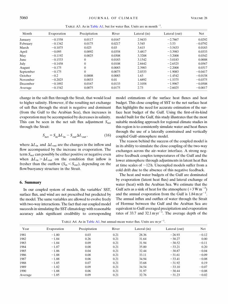
TABLE A3. As in Table A1, but for water flux. Units are m month21.
Month Evaporation Precipitation River Lateral (in) Lateral (out) Net
January 20.1558 0.0117 0.0167 2.9433 22.7867 0.0292
February 20.1342 0.0175 0.0217 3.545 23.53 20.0792
March 20.1075 0.025 0.03 3.615 23.5433 0.0183
April 20.095 0.0092 0.0358 3.4817 23.3983 0.0333
May 20.1192 0.0025 0.0308 3.3208 23.2008 0.0342
June 20.1533 0 0.0183 3.1542 23.0183 0.0008
July 20.1458 0 0.0108 2.8442 22.6525 0.0567
August 20.175 0 0.0083 2.3983 22.2008 0.0317
September 20.175 0 0.0075 2.0333 21.9083 20.0417
October 20.2 0.0008 0.0083 1.63 21.4542 20.0158
November 20.2025 0.0033 0.01 1.6892 21.5375 20.0375
December 20.1892 0.0167 0.0133 2.1058 21.9967 20.0508
Average 20.1542 0.0075 0.0175 2.73 22.6025 20.0017
TABLE A4. As in Table A1, but annual-mean water flux. Units are m yr21.
Year Evaporation Precipitation River Lateral (in) Lateral (out) Net
1981 21.80 0.03 0.21 28.36 226.93 20.12
1982 21.84 0.26 0.21 31.64 230.27 0.00
1983 21.84 0.09 0.21 31.94 230.52 20.11
1984 21.87 0.08 0.21 35.00 233.21 0.20
1985 21.86 0.04 0.21 32.44 230.87 20.04
1986 21.88 0.08 0.21 33.11 231.61 20.09
1987 21.88 0.06 0.21 34.94 233.41 20.08
1988 21.85 0.07 0.21 33.68 231.92 0.19
1989 21.82 0.09 0.21 34.54 233.10 20.07
1990 21.88 0.06 0.21 31.97 230.44 20.08
Average 21.85 0.09 0.21 32.76 231.23 20.02
5060 JOURNAL OF CL IMATE VOLUME 28
Gulf water is ;38m. Hence, we estimate that the mean
residency time scale for the entire Gulf is;14 months.
Acknowledgments. This work was funded under the
Cooperative Agreement between the Masdar Institute
of Science and Technology (Masdar Institute), Abu
Dhabi, UAE, and the Massachusetts Institute of Tech-
nology (MIT), Cambridge, MA, USA–Reference 02/
MI/MI/CP/11/07633/GEN/G/00. Xue’s research was
also supported by the Michigan Tech Research Excel-
lence Fund Research Seed Grant. This is also research
(Contribution No. 19) of the Great Lakes Research
Center at Michigan Tech. The authors thank Dr. Marc
Marcella and Dr. Im Eun Soon for their help with
atmosphere-only model configuration. We also thank
three anonymous reviewers’ valuable comments, which
have greatly helped us to improve this research. E. E.
and P. X. conceived and designed the experiments; P. X.
performed the modeling experiments; E. E. and P. X.
analyzed the data; andE. E. and P. X. cowrote the paper.
APPENDIX
Estimates of Water and Heat Fluxes from GARMwith ERA-40 Atmospheric Boundary
Basin-averaged, climatological, monthly and annual
heat and water fluxes for theGulf, 1981–90, estimated by
the Gulf–atmosphere model with ERA-40 atmospheric
boundary (Tables A1–A4).
REFERENCES
Abualnaja, Y., 2009: Estimation of the net surface heat flux in the
Arabian Gulf based on the equilibrium temperature. J. King
Abdulaziz Univ. Mar. Sci., 20, 21–29, doi:10.4197/Mar.20-1.2.
Ahmad, F., and S. A. R. Sultan, 1991: Annual mean surface heat
fluxes in the Arabian Gulf and the net heat transport through
the Strait of Hormuz. Atmos.–Ocean, 29, 54–61, doi:10.1080/
07055900.1991.9649392.
Antonov, I., 2010: Salinity.Vol. 2,WorldOceanAtlas 2009,NOAA
Atlas NESDIS 69, 184 pp.
Beardsley, R. C., C. Chen, and Q. Xu, 2013: Coastal flooding in Scituate
(MA): A FVCOM study of the 27 December 2010 nor’easter.
J.Geophys.Res.Oceans,118,6030–6045,doi:10.1002/2013JC008862.
Buck, A. L., 1981: New equations for computing vapor pressure
and enhancement factor. J. Appl. Meteor., 20, 1527–1532,
doi:10.1175/1520-0450(1981)020,1527:NEFCVP.2.0.CO;2.
Carton, J. A., and B. S. Giese, 2008: A reanalysis of ocean climate
using Simple Ocean Data Assimilation (SODA). Mon. Wea.
Rev., 136, 2999–3017, doi:10.1175/2007MWR1978.1.
Chao, S., T. W. Kao, and K. R. Al-Hajri, 1992: A numerical in-
vestigation of circulation in the Arabian Gulf. J. Geophys.
Res., 97, 11 219–11 236, doi:10.1029/92JC00841.Chen,C.,H.Liu, andR.C.Beardsley, 2003:Anunstructuredgrid, finite-
volume, three-dimensional, primitive equations ocean model:
Application to coastal ocean and estuaries. J. Atmos. Oceanic
Technol., 20, 159–186, doi:10.1175/1520-0426(2003)020,0159:
AUGFVT.2.0.CO;2.
——, R. C. Beardsley, and G. Cowles, 2006: An unstructured grid,
Finite-Volume Coastal Ocean Model (FVCOM) system.
Oceanography, 19, 78–89, doi:10.5670/oceanog.2006.92.
——, and Coauthors, 2008: Physical mechanisms for the offshore
detachment of the Changjiang diluted water in the East China
Sea. J. Geophys. Res., 113,C02002, doi:10.1029/2006JC003994.
——, Z. Lai, R. C. Beardsley, J. Sasaki, J. Lin, H. Lin, R. Ji, and
Y. Sun, 2014: The March 11, 2011 T�ohoku M9.0 earthquake-
induced tsunami and coastal inundation along the Japanese
coast: A model assessment. Prog. Oceanogr., 123, 84–104,
doi:10.1016/j.pocean.2014.01.002.
Cowles, G. W., S. J. Lentz, C. Chen, Q. Xu, and R. C. Beardsley,
2008: Comparison of observed and model-computed low fre-
quency circulation and hydrography on the New England
shelf. J. Geophys. Res., 113, C09015, doi:10.1029/
2007JC004394.
Evans, J. P., R. B. Smith, and R. J. Oglesby, 2004: Middle East
climate simulation and dominant precipitation processes. Int.
J. Climatol., 24, 1671–1694, doi:10.1002/joc.1084.
Fairall, C. W., E. F. Bradley, D. P. Rogers, J. B. Edson, and G. S.
Young, 1996: Bulk parameterization of air-sea fluxes for
tropical ocean-global atmosphere coupled-ocean atmosphere
response experiment. J. Geophys. Res., 101, 3747–3764,
doi:10.1029/95JC03205.
Gianotti, R. L., 2013: Convective cloud and rainfall processes over
the Maritime Continent: Simulation and analysis of the di-
urnal cycle. Ph.D. thesis, Massachusetts Institute of Technol-
ogy, 307 pp.
——, and E. A. B. Eltahir, 2014a: Regional climate modeling over
the Maritime Continent. Part I: New parameterization for
convective cloud fraction. J. Climate, 27, 1488–1503,
doi:10.1175/JCLI-D-13-00127.1.
——, and ——, 2014b: Regional climate modeling over the
Maritime Continent. Part II: New parameterization for
autoconversion of convective rainfall. J. Climate, 27, 1504–
1523, doi:10.1175/JCLI-D-13-00171.1.
Giorgi, F., and L. O. Mearns, 1999: Introduction to special section:
Regional climate modeling revisited. J. Geophys. Res., 104,
6335–6352, doi:10.1029/98JD02072.
Hamza, W., and M. Munawar, 2009: Protecting and managing the
ArabianGulf: Past, present and future.Aquat. Ecosyst. Health
Manage., 12, 429–439, doi:10.1080/14634980903361580.
Hassanzadeh, S., F. Hosseinibalam, and A. Rezaei-Latifi, 2011:
Numerical modelling of salinity variations due to wind and
thermohaline forcing in the PersianGulf.Appl.Math.Modell.,
35, 1512–1537, doi:10.1016/j.apm.2010.09.029.
——,——, and——, 2012: Three-dimensional numerical modeling
of the water exchange between the Persian Gulf and the Gulf
of Oman through the Strait of Hormuz. Oceanol. Hydrobiol.
Stud., 41, 85–98, doi:10.2478/s13545-012-0010-6.
Hastenrath, S., P. J. Lamb, and L. L. Greischar, 1979: Climatic
Atlas of the Indian Ocean: The Oceanic Heat Budget. Uni-
versity of Wisconsin Press, 93 pp.
Johns,W. E., F. Yao, D. B. Olson, S. A. Josey, J. P. Grist, andD. A.
Smeed, 2003: Observations of seasonal exchange through the
Straits of Hormuz and the inferred heat and freshwater bud-
gets of the Persian Gulf. J. Geophys. Res., 108, 3391,
doi:10.1029/2003JC001881.
Kämpf, J., and M. Sadrinasab, 2006: The circulation of the Persian
Gulf: A numerical study. Ocean Sci., 2, 27–41, doi:10.5194/
os-2-27-2006.
1 JULY 2015 XUE AND ELTAH IR 5061
Locarnini, A., 2010: Temperature. Vol. 1,World Ocean Atlas 2009,
NOAA Atlas NESDIS 68, 184 pp.
Marcella, M. P., and E. A. B. Eltahir, 2008: The hydroclimatology
of Kuwait: Explaining the variability of rainfall at seasonal and
interannual time scales. J. Hydrometeor., 9, 1095–1105,
doi:10.1175/2008JHM952.1.
——, and ——, 2012: Modeling the summertime climate of
Southwest Asia: The role of land surface processes in shaping
the climate of semiarid regions. J. Climate, 25, 704–719,
doi:10.1175/2011JCLI4080.1.
——, and——, 2014: Introducing an irrigation scheme to a regional
climate model: A case study over West Africa. J. Climate, 27,5708–5723, doi:10.1175/JCLI-D-13-00116.1.
Mellor, G. L., and T. Yamada, 1982: Development of a turbulence
closure model for geophysical fluid problems. Rev. Geophys.,
20, 851–875, doi:10.1029/RG020i004p00851.
Meshal, A. H., and H. M. Hassan, 1986: Evaporation from the
coastal waters of the central part of the Gulf.Arab Gulf J. Sci.
Res., 4, 649–655.Pal, J. S., and Coauthors, 2007: Regional climate modeling for the
developing world: The ICTP RegCM3 and RegCNET. Bull.
Amer. Meteor. Soc., 88, 1395–1409, doi:10.1175/
BAMS-88-9-1395.
Prasad, T. G., M. Ikeda, and S. P. Kumar, 2001: Seasonal spreading
of the PersianGulf watermass in theArabian Sea. J. Geophys.
Res., 106, 17 059–17 071, doi:10.1029/2000JC000480.Privett, D. W., 1959: Monthly charts of evaporation from the N.
Indian Ocean (including the Red Sea and the Persian Gulf).
Quart. J. Roy. Meteor. Soc., 85, 424–428, doi:10.1002/
qj.49708536614.
Reynolds, R. M., 1993: Physical oceanography of the Gulf, Strait of
Hormuz, and theGulf ofOman—Results from theMtMitchell
expedition. Mar. Pollut. Bull., 27, 35–59, doi:10.1016/
0025-326X(93)90007-7.
Reynolds, R. W., T. M. Smith, C. Liu, D. B. Chelton, K. S. Casey,
and M. G. Schlax, 2007: Daily high-resolution-blended
analyses for sea surface temperature. J. Climate, 20, 5473–5496, doi:10.1175/2007JCLI1824.1.
Saad, M. A. H., 1978: Seasonal variations of some physicochemical
conditions of Shatt al-Arab estuary, Iraq. Estuarine Coastal
Mar. Sci., 6, 503–513, doi:10.1016/0302-3524(78)90027-0.Sabziparvar, A. A., S. H. Mirmasoudi, H. Tabari, M. J.
Nazemosadat, and Z. Maryanaji, 2011: ENSO teleconnection
impacts on reference evapotranspiration variability in some
warm climates of Iran. Int. J. Climatol., 31, 1710–1723,
doi:10.1002/joc.2187.
——, R. Mousavi, S. Marofi, N. Ebrahimipak, and M. Heidari,
2013: An improved estimation of the Angstrom–Prescott ra-
diation coefficients for the FAO56 Penman–Monteith
evapotranspiration method. Water Resour. Manage., 27,
2839–2854, doi:10.1007/s11269-013-0318-z.
Sadrinasab, M., and J. Kämpf, 2004: Three-dimensional flushing
times of the Persian Gulf. Geophys. Res. Lett., 31, L24301,
doi:10.1029/2004GL020425.
Sale, P., and Coauthors, 2011: The growing need for sustainable
ecological management of marine communities of the Persian
Gulf. Ambio, 40, 4–17, doi:10.1007/s13280-010-0092-6.
Saleh, D., 2010: Stream gage descriptions and streamflow statistics
for sites in the Tigris River and Euphrates River basins, Iraq.
U.S. Geological Survey Data Series 540, 146 pp.
Sheppard, C., and Coauthors, 2010: The Gulf: A young sea in decline.
Mar. Pollut. Bull., 60, 13–38, doi:10.1016/j.marpolbul.2009.10.017.
Shirvani, A., S. M. J. Nazemosadat, and E. Kahya, 2014: Analyses
of the Persian Gulf sea surface temperature: Prediction and
detection of climate change signals. Arabian J. Geosci., 8,
2121–2130, doi:10.1007/s12517-014-1278-1.
Smagorinsky, J., 1963: General circulation experiments with the
primitive equations. Mon. Wea. Rev., 91, 99–164, doi:10.1175/1520-0493(1963)091,0099:GCEWTP.2.3.CO;2.
Sofianos, S. S., W. E. Johns, and S. P. Murray, 2002: Heat and
freshwater budgets in the Red Sea from direct observations at
Bab el Mandeb. Deep-Sea Res. II, 49, 1323–1340, doi:10.1016/S0967-0645(01)00164-3.
Thoppil, P. G., and P. J. Hogan, 2010: A modeling study of circu-
lation and eddies in the Persian Gulf. J. Phys. Oceanogr., 40,2122–2134, doi:10.1175/2010JPO4227.1.
Tian, R., and C. Chen, 2006: Influence of model geometrical fitting
and turbulence parameterization on phytoplankton simulation
in the Gulf of Maine. Deep-Sea Res. II, 53, 2808–2832,
doi:10.1016/j.dsr2.2006.08.006.
Tragou, E., C. Garrett, R. Outerbridge, and C. Gilman, 1999: The
heat and freshwater budgets of the Red Sea. J. Phys. Ocean-
ogr., 29, 2504–2522, doi:10.1175/1520-0485(1999)029,2504:
THAFBO.2.0.CO;2.
Valcke, S., 2013: The OASIS3 coupler: A European climate
modelling community software. Geosci. Model Dev., 6, 373–388, doi:10.5194/gmd-6-373-2013.
Weisberg, R. H., and L. Zheng, 2006: Circulation of Tampa Bay
driven by buoyancy, tides, and winds, as simulated using a fi-
nite volume coastal ocean model. J. Geophys. Res., 111,C01005, doi:10.1029/2005JC003067.
Winter, J. M., J. S. Pal, and E. A. B. Eltahir, 2009: Coupling of in-
tegrated biosphere simulator to regional climate model version
3. J. Climate, 22, 2743–2757, doi:10.1175/2008JCLI2541.1.Xue, P., C. Chen, P. Ding, R. C. Beardsley, H. Lin, J. Ge, and
Y. Kong, 2009: Saltwater intrusion into the Changjiang River:
A model-guided mechanism study. J. Geophys. Res., 114,C02006, doi:10.1029/2008JC004831.
——, ——, R. C. Beardsley, and R. Limeburner, 2011: Observing
system simulation experiments with ensemble Kalman filters
in Nantucket Sound, Massachusetts. J. Geophys. Res., 116,C01011, doi:10.1029/2010JC006428.
——, E. A. B. Eltahir, P. Malanotte-Rizzoli, and J. Wei, 2014:
Local feedback mechanisms of the shallow water region
around theMaritime Continent. J. Geophys. Res. Oceans, 119,6933–6951, doi:10.1002/2013JC009700.
Yao, F., andW. E. Johns, 2010a: AHYCOMmodeling study of the
Persian Gulf: 1. Model configurations and surface circulation.
J. Geophys. Res., 115, C11017, doi:10.1029/2009JC005781.——, and ——, 2010b: A HYCOM modeling study of the Persian
Gulf: 2. Formation and export of Persian Gulf Water.
J. Geophys. Res., 115, C11018, doi:10.1029/2009JC005788.Zeng,X.,M.Zhao, andR.E.Dickinson, 1998: Intercomparisonof bulk
aerodynamic algorithms for the computation of sea surface fluxes
using TOGACOARE and TAO data. J. Climate, 11, 2628–2644,
doi:10.1175/1520-0442(1998)011,2628:IOBAAF.2.0.CO;2.
Zhao, L., C. Chen, J. Vallino, C. Hopkinson, R. C. Beardsley, H. Lin,
and J. Lerczak, 2010: Wetland-estuarine-shelf interactions in the
Plum Island Sound and Merrimack River in the Massachusetts
coast. J. Geophys. Res., 115, C10039, doi:10.1029/2009JC006085.
5062 JOURNAL OF CL IMATE VOLUME 28