Solar Energy Vol. 28, No. 4, pp. 293--302, 1982 003g-092X/$2/040293.-10503.00/0 Printed in Great Bri~in, © 19~2 Pergamon Press Ltd.

ESTIMATION OF THE DIFFUSE RADIATION FRACTION FOR HOURLY, DAILY AND MONTHLY-AVERAGE

GLOBAL RADIATION

D. G. ERAS, S. A. KLEIN and J. A. DUFFLE Solar Energy Laboratory, University of Wisconsin, Madison, WI 53706, U.S.A.

(Received 1 May 1981; accepted 18 August 1981)

Abstract--Hourly pyrheliometer and pyranometer data from four U.S. locations are used to establish a relationship between the hourly diffuse fraction and the hourly clearness index kr. This relationship is compared to the relationship established by Orglll and Hollands and to a set of data from Highett, Australia, and agreement is within a few percent in both cases. The transient simulation program TRNSYS is used to calculate the annual performance of solar energy systems using several correlations. For the systems investigated, the effect of simulating the random distribution of the hourly diffuse fraction is negligible. A seasonally dependent daily diffuse correlation is developed from the data, and this daily relationship is used to derive a correlation for the monthly-average diffuse fraction.

1. INTRODUCTION

Solar radiation incident on buildings or collection sur- faces must be known in order to perform thermal analyses. In general, only measurements of the total horizontal (global) radiation are available. As most sur- faces of interest are inclined, it is necessary to estimate the radiation on a tilted surface from measurements of global radiation. Estimation procedures usually require the beam and diffuse components of global radiation.

The beam and diffuse components of global radiation can be estimated from empirical relationships. Existing relationships correlate the fraction of the global radiation which is beam or diffuse to an index of atmospheric clarity. Correlations of this type have been developed for use with hourly, daily, and monthly-average values of global radiation.

The hourly correlations of Boes[1], Orgill and Hollands [2], and Bruno [3] can be expressed as relation- ships of ISL the ratio of the hourly diffuse radiation to the hourly global radiation, to kT, the ratio of the hourly global radiation to the hourly extraterrestrial radiation, IIIo. Correlations of the hourly diffuse fraction, Ia]L to kc, the ratio of the hourly global radiation to an estimate of hourly "clear sky" radiation, IIIc, have been developed by Bugler[4] and by Stauter and Klein[5], each with different definitions of "clear sky" radiation. The statistical algorithm developed by Randall and Whitson[6] cannot be expressed analytically; this al- gorithm was used[7] to estimate beam radiation for the SOLMET data base.

Relationships for estimating the beam and diffuse components of daily global radiation have also been developed by numerous authors. The correlations of Liu and Jordan[8], Choudhury[9], Stanhill[10], Tuller [ l l ], Ruth and Chant[12], and Collares-Pereira and Rabl[13] all relate HSH, the daily diffuse fraction, to Kr, the ratio of daily global to daily extra-terrestrial radiation, H/Ho.

On a monthly-average basis, relationships between HaJH and /(T have been developed by Liu and Jordan[8], Page[14], Tuller [l l ], Collares-Pereira and Rabl [13], and Iqbal [ 15]. Hay [ 16] developed a correlation

which includes the effect of multiple reflections between the ground and sky.

Within each group of existing correlations (i.e. the hourly, daily, and monthly-average relationships) there is considerable disagreement. The significance of this dis- agreement depends upon what the diffuse correlation is used for. If the annual total radiation on a tilted surface is estimated using each of the existing relationships, the results will generally be within a few percent. If a computer simulation is used to estimate the annual per- formance of a system with concentrating collectors, the results obtained using different correlations may vary by more than 10 per cent. In addition, there are incon- sistencies between daily and monthly correlations. These discrepancies may be the result of variations in in- strumentation and measurement techniques, different methods of correlating the data, locational dependence of the data, or insufficient data.

The objectives of this study are to develop, from a new data base, relationships for estimating the diffuse fraction of hourly, daily, and monthiy-average global radiation, to determine the degree to which the relation- ships developed are dependent on season and location, and to compare these relationships to the existing rela- tionships.

2. THE DATA BASE

The data used to develop the correlations presented here are thought to be among the best data available at this time. These data were recorded at the four U.S. cities listed in Table 1. The data for Livermore were recorded by Sandia; those for Raleigh by the Environ- mental Protection Agency; and the data from Fort Hood and Maynard were recorded by the Army Atmospheric Sciences Laboratory. The Aerospace Corporation edited the raw data, reduced them to the International Pyr- heliometric Scale, and placed them on magnetic tape. Information included for each hour are direct normal radiation, total radiation, mean solar altitude, declination, date, and extraterrestrial radiation. The direct normal radiation was measured with a pyrheliometer and the

293

294 D. G. Exns et al.

Table 1. Cities and duration of records for aerospace data base

Fort Hood, Livermore, Raleigh, Maynard, Albuquerque, Stat ion Name TX CA NC MA NM

S t a t i o n Number

L a t i t u d e (Deg. N~

Longitude (Deg. N)

Altitude (ft)

Data Period

Begin

End

( D a y / l ~ / Y r )

03902 32899

31.08 37.70

97.85 121.70

1080 486

119174 118174

3016178 30110175

32900

35.87

78.78

441

20/3/75

114176

-0042

42.42

71.48

203

111175

31112/76

23050

35.05

106.62

5314

1/1/81

31/12/84

total radiation was measured with a pyranometer. It should be noted that while the use of a pyrheliometer eliminates the needs for shade ring corrections, there can be problems with tracking systems and calibration.

To test the applicability of the correlation at locations other than the four from which it was derived, a set of data recorded in Highett, Victoria, Australia (latitude 38'S) during the years 1966--69 was obtained[17]. These data, measured using an unshaded pyranometer and a pyranometer with a shade ring, are also thought to be of high quality.

In addition, hourly data for a month (Feb. 1980) recorded in Albany, NY were obtained from the Atmospheric Sciences Research Center of the State University of New York[18]. These data are numerical integrations of minute values. Included in this data set are total insolation on a horizontal surface, direct normal insolation, diffuse insolation using a shadow band, diffuse insolation using an occulting disk, and the number of minutes of beam radiation during each hour. The presence of three independent measurements of the diffuse radiation made it possible to monitor the internal consistency of the diffuse data.

All of the data were checked for the following in- consistencies: zero global radiation after sunrise and before sunset, beam radiation exceeding global, global radiation exceeding extraterrestrial, and no beam radia- tion when kr is large. Data exhibiting any of these problems (less than 1 per cent of the total number of hours) were deleted from the data set.

3. ESTIMATING T I ~ DIFFUSE FRACTION OF HOURLY GLOBAL

RADIATION

(a) Correlating the diffuse fraction with kr The diffuse fraction of the hourly total radiation is

strongly correlated with kr [8,2,3]. The parameter kr is an indicator of the relative clearness of the atmosphere. In general, when the atmosphere is clearer, a smaller fraction of the radiation is scattered. A relationship was developed between Idl and kr using the combined data of the four U.S. locations. The individual kr and Ia/l values were weighted with the total radiation for the hour, and average values calculated for each interval in

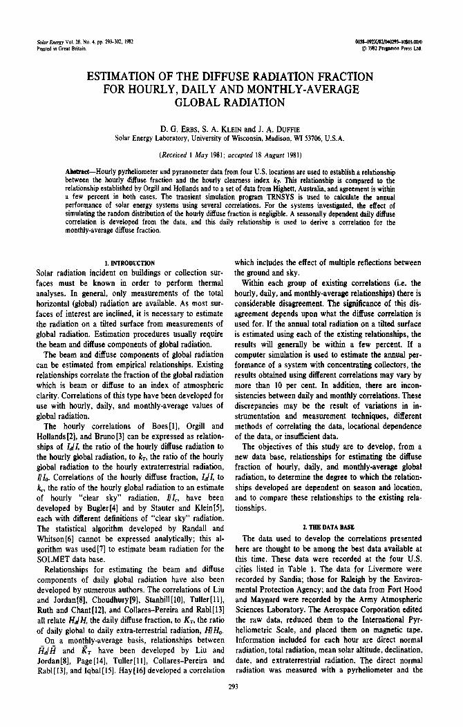
kT of 0.025. The resulting correlation is shown with the average data in Fig. 1. It can be represented by:

IJI = 1.0 - 0.09 kr for kr <- 0.22

la]l = 0.9511 - 0.1604 kr + 4.388 k 2 - 16.638 k3r + 12.336 k~-for 0.22 < kr <-0.80

Ia/I = 0.165 for kr > 0.80. (1)

For values of kT greater than 0.8, eqn (1) was not fit to the data. Following the procedure of Orgill and Hollands[2], a constant value of IJI was chosen for kT in this range. Orgill and Hollands attribute the observed increase in the diffuse fraction as kr increases from 0.8 to beam radiation being reflected from clouds and recorded as diffuse radiation during periods when the sun is unobscured by the surrounding clouds. The data in this region of kT represent only 0.2 per cent of the points in the combined data set, and they are not under- stood well enough to justify fitting a curve to them.

The mean bias error (d) and the standard deviation (~r) are used to indicate how closely the hourly correlation agrees with the data. The mean bias error is the weighted difference between the diffuse fractions estimated from a correlation and the measured diffuse fractions.

N

( ( I , d / ) - ( I , , . . , / / ) ) 1

d = N (2) 5"./

1.2 L, , . a ' , ' I ' , ' I ' , ' I ' , ' i ' ,~e' , ' I ' , ' q r r T m T ' ~

All Locations

65 Months Data

I 1 " ~ N × --

XXX

i,i,l,I,t,t,i,I,L,l,i,l,t,L,i,l~L,ILtJ -0.[j . I .2 .3 .4 -5 .6 .7 .8 .8 1 .0

kr Fig. 1. Hourly correlation between I~II and kr compared to average

hourly U.S. data.

Estimation of the diffuse radiation fraction for global radiation

In eqn (2), Id.,, is the measured diffuse radiation, I is the measured total radiation, and la.c is the diffuse radiation estimated from the correlation. The standard deviation is an indication of how much the measured hourly diffuse fractions vary from the correlation. The standard devia- tion is defined by:

1 ' 2 - ' ' ' 1 ' ' ' 1 ' ~ ' 1 ' ~ ' 1 ' ~ ' 1 ' . I ' ' ' 1 ' ' ' 1 ' ' ' 1 '

o" = ,/z (3)

In general, 95 per cent of the data lie within plus and minus 2~r of the correlation.

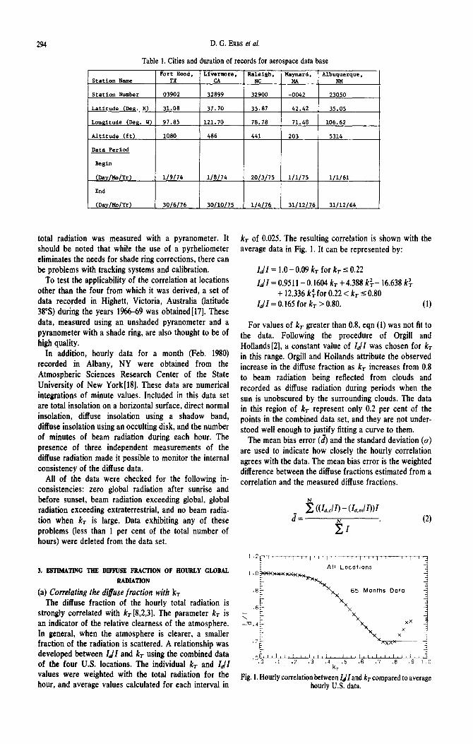
The mean bias error and standard deviation were calculated for the data from each of the four U.S. locations. Figure 2 shows the hourly correlation (solid line), average values of the data for each interval in kr of 0.0125 (x's), and plus and minus one standard deviation of the hourly diffuse fractions from the correlation (dashed lines). The mean bias error exhibits only a slight Iocational dependence, and except for Livermore, the average data lie very close to the correlation for all values of kr less than 0.8. The standard deviation is also relatively independent of location. However, the lane size of the standard deviation indicates that there may be considerable error (roughly plus or minus two standard deviations) in estimating the diffuse fraction for any particular hour.

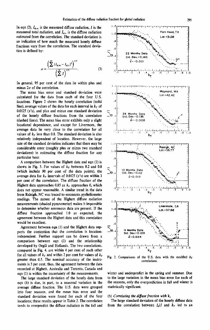
A comparison between the Highett data and eqn (I) is shown in Fig. 3. For values of kr between 0.2 and 0.8 (which include 90 per cent of the data points), the average data for kr intervals of 0.0125 (x's) are within 3 per cent of the correlation. The diffuse fraction of the Highett data approaches 0.85 as kr approaches 0, which does not appear reasonable. A similar trend in the data from Raleigh, NC was traced to erroneous pyrheliometer readings. The nature of the ttighett diffuse radiation measurements (shaded pyranometer) makes it impossible to determine whether erroneous data are present. If the diffuse fraction approached 1.0 as expected, the agreement between the Highett data and this correlation would be excellent.

Agreement between eqn (1) and the ttighett data sup- ports the contention that the correlation is location- independent. Further support can be drawn from a comparison between eqn (1) and the relationship developed by Orgill and Hollands. The two correlations, compared in Fig. 4, are within 4 per cent of each other for all values of kr and within 2 per cent for values of kr greater than 0.5. The nominal accuracy of the instru- ments is 5 per cent; thus, the agreement between the data recorded at Highett, Australia and Toronto, Canada and eqn (I) is within the uncertainty of the measurements.

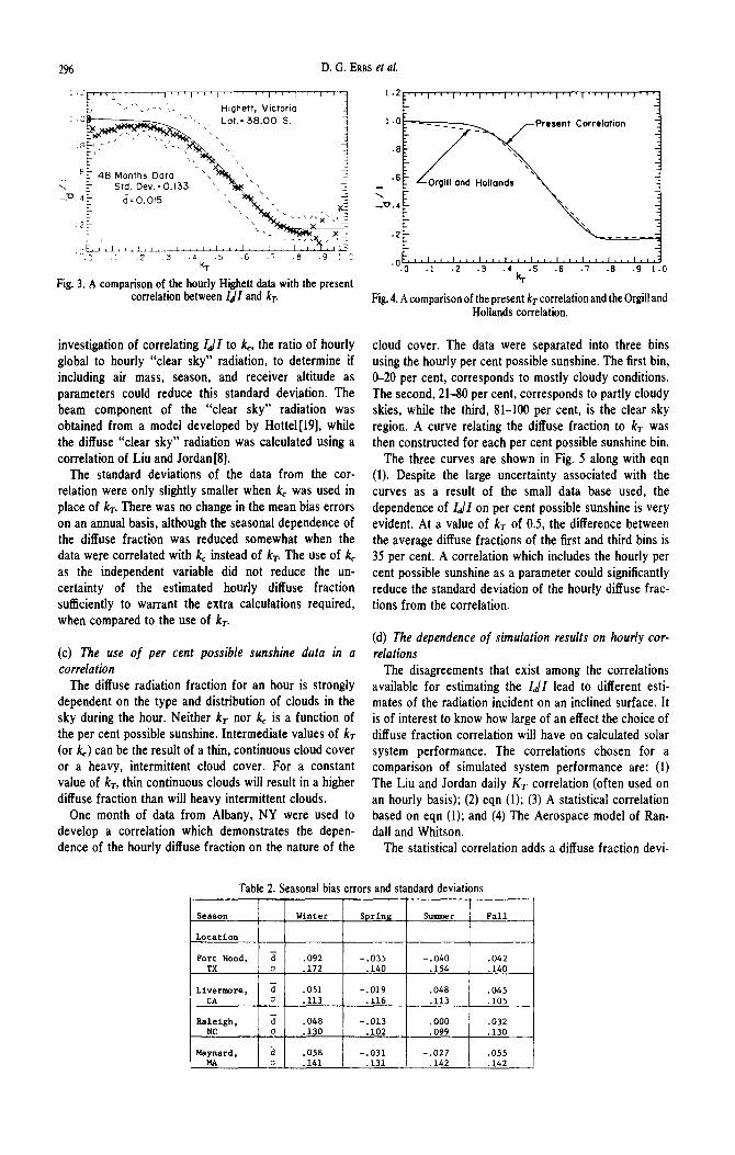
The large standard deviation of the hourly data from eqn (1) is due, in part, to a seasonal variation in the average diffuse fraction. The U.S. data were grouped into four seasons, and the mean bias error and the standard deviation were found for each of the four locations; these results appear in Table 2. The correlation tends to overpredict the diffuse radiation in the fall and

295

. F o r t H o o d , T X

:- . . . . . . ~ - - . L o t . • 3 1 . 0 8

2 2 M o n t " \ ~

~ ' U . , S t d . O e v . = 0 A 4 3 ~ ~ ~_

. 0 . 0 I ' l ' i ' I ' ~ , I , I , -L -~ I , i , l , I , , I , I , I . I ,~ • 1 . 2 .3 .4 . 5 .6 . ? . 8 . 9

k T 1.0

1,0

.8

.6

.2

,t] • [J

' 7 ~ T ~ r ~ q - ' r T ' T ~ - - ~ T T T T T ' I i , I q ~ ' T - r - r ~ F r l T ' r ~

, , ' ~ M o y n o r d . M A

~ : , L o t . - 4 2 . 4 2

- \ \ \ a \

2 4 M o n t h s " .

S'd' ° t~ '=°"~ '7 "~.~, - o . o o e - \ . ~ , ~ ; ~

, , ~ ~ L ~ .~_~_1 ~ L J _ ~ I = d ~ _ L ~ J ~ L . 4 -~J_A_ ;=&_~L .1 . : : . 3 .4 ,S . 6 .'? , 8 . 9 . 0

kT

I , 2 : q r ~ T ' ~ ' q ~ q - , [ , I ' [ ' "I ' I ' I ' I ~ ' q ' ~ 7 - r T ~ ' f ~

: ,~ R o l e gh NC ! . 0 ~ : ~ . 7 , ~ , L o t . = 3 5 . 7 7

• 6 \ k

I0 Months ' " ' _~. , S,d O_ev..O,,2 " ' . ~ i '

. .~ . I , , , I , ~I ._~.4_~L~_J_ l , I , L , l , I ,~L , I . J " 0 , 0 .I , 2 , 3 , 4 ,S , 6 , 7 . 8 , 9 ! - 0

k T

1 . 2 i . l . , , l , i , l . i , l . , . l , , i , , , i , i l , i , l , ,

I'L L i v e r m o r e , CA l . O ~ ~ , L O t . - 3 7 . 6 8

I I M o n t h s D a t a ~ . ~ ~ h ~ - - - L, \ I t~" _ _ ' U . 4 S ia l . D e v . - O . 1 0 9 ~ / , ( ' Y x ' ~ , , •

o = v.v.3"eo v.v.3,,e % " ~ ,..3(x)~

~ , ~ -I

I , I , I , I *1 , J , I , l . l . I , I , 1 . 1 , [ , i , I , l l l , l , 1 , 4 " 0 . 0 . l . 2 . 3 . 4 . 5 . 6 . 7 . 8 . 9 1 . 0

k T

Fig. 2. Comparisons of the U.S. data with the modified kr correlations.

winter and underpredict in the spring and summer. Due to the large variation in the mean bias error for each of the seasons, only the overprediction in fall and winter is statistically significant.

(b) Correlating the diffuse fraction with k~ The large standard deviation of the hourly diffuse data

from the correlation between Ia]I and kr led to an

296 D.G. ERBS

i . ~ , ~ . , . , , . , . , . , . . , . , . , . , . , . , . , . , . , . , - ~ ~ "~ " . ~ ~ ' ~ Highett, Victoria 4

i .0~. ~ - " , , L a t = 5 8 . O 0 S.

-- - 6 ~ \ -:- Sld. Dev. : 0.133 \ x ~ , -~. ~ :_- c~:o.o~ \ % ' ,

• Z~ ×\

• .0 . I .2 .3 .4 -5 ,6 .7 -8 .9 : .2 kT

Fig. 3. A comparison of the hourly Highett data with the present correlation between I,/I and kr.

et al.

l .O . . . . = ~ r e s e n t Correlation

.6

--'~.4

• 2 . . . . . .

,0.0 l l J ' l ' l ' J ' l ' q l l ' i ' l ' ' ' l ~ ' ' l ' l ' l ' ' l l ~ l A • 1 .2 -3 .4 k r .5 ,6 .7 .8 .9 1.0

Fig. 4. A comparison of the present kr correlation and the Orgill and Hollands correlation.

investigation of correlating IdI to ko the ratio of hourly global to hourly "clear sky" radiation, to determine if including air mass, season, and receiver altitude as parameters could reduce this standard deviation. The beam component of the "clear sky" radiation was obtained from a model developed by Hottel[19], while the diffuse "clear sky" radiation was calculated using a correlation of Liu and Jordan[8].

The standard deviations of the data from the cor- relation were only slightly smaller when k~ was used in place of kr. There was no change in the mean bias errors on an annual basis, although the seasonal dependence of the diffuse fraction was reduced somewhat when the data were correlated with kc instead of kr. The use of kc as the independent variable did not reduce the un- certainty of the estimated hourly diffuse fraction sufficiently to warrant the extra calculations required, when compared to the use of kr.

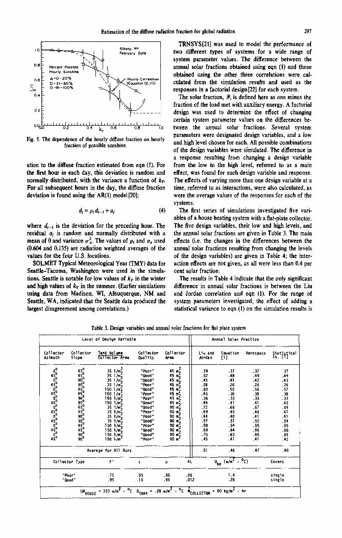
(c) The use o /per cent possible sunshine data in a correlation

The diffuse radiation fraction for an hour is strongly dependent on the type and distribution of clouds in the sky during the hour. Neither kr nor kc is a function of the per cent possible sunshine. Intermediate values of kr (or kc) can be the result of a thin, continuous cloud cover or a heavy, intermittent cloud cover. For a constant value of kr, thin continuous clouds will result in a higher diffuse fraction than will heavy intermittent clouds.

One month of data from Albany, NY were used to develop a correlation which demonstrates the depen- dence of the hourly diffuse fraction on the nature of the

cloud cover. The data were separated into three bins using the hourly per cent possible sunshine. The first bin, 0-20 per cent, corresponds to mostly cloudy conditions. The second, 21--80 per cent, corresponds to partly cloudy skies, while the third, 81-100 per cent, is the clear sky region. A curve relating the diffuse fraction to kT was then constructed for each per cent possible sunshine bin.

The three curves are shown in Fig. 5 along with eqn (1). Despite the large uncertainty associated with the curves as a result of the small data base used, the dependence of IdI on per cent possible sunshine is very evident. At a value of kr of 0.5, the difference between the average diffuse fractions of the first and third bins is 35 per cent. A correlation which includes the hourly per cent possible sunshine as a parameter could significantly reduce the standard deviation of the hourly diffuse frac- tions from the correlation.

(d) The dependence o[ simulation results on hourly cor- relations

The disagreements that exist among the correlations available for estimating the Id l lead to different esti- mates of the radiation incident on an inclined surface. It is of interest to know how large of an effect the choice of diffuse fraction correlation will have on calculated solar system performance. The correlations chosen for a comparison of simulated system performance are: (1) The Liu and Jordan daily Kr correlation (often used on an hourly basis); (2) eqn (1); (3) A statistical correlation based on eqn (1); and (4) The Aerospace model of Ran- dall and Whitson.

The statistical correlation adds a diffuse fraction devi-

Table 2. Seasonal bias errors and standard deviations

Season

L o c a t i o n

For t Hood, TX

Livermore, CA

Raleigh, NC

Maynard, MA

Winter

.092 a .172

.o51 a .113

.048 c .130

.058 o .141

Sprin 8 Summer Fall

-.035 -.040 .042 .140 .154 .140

-.019 .048 .045 .116 .113 .105

-.013 .000 .032 .102 .099 .130

-.027 .142

-.031 .131

.055

.142

Estimation of the diffuse radiation fraction for global radiation 297

1.0 -- -~,-',~¢=-~-~L~ J , i Albony, NY F:ebruar y Ooto

O.e Percent Possible [ ~ ' ~ L l e Hourly ?un=shlne i I ~

0.6 A =0-20% x\ T - ~ L/--Hourly Correlation O=2t-80% \1 i ~ ( E q u o t i o n (2.1l))

-~0 O "8' - '00"/. " 1 ~ / i ~ , E L 0.4

0,2 . . . .

0.00~ 0 I ' 1 ' 1 ' l ' l ' l ' l ' l ' l l l ~ l ' l ' l ' l ' l ' l l l ' l ' l J 0.2 0.4 ~ 046 ON8 ~.0

Fig. 5. The dependence of the hourly diffuse fraction on hourly fraction of possible sunshine.

ation to the diffuse fraction estimated from eqn (1). For the first hour in each day, this deviation is random and normally distributed, with the variance a function of kT. For all subsequent hours in the day, the diffuse fraction deviation is found using the AR(I) model[20]:

d~=p, dj_,+ay (4)

where dj_, is the deviation for the preceding hour. The residual aj is random and normally distributed with a mean of 0 and variance 2 (to. The values of p, and o,o used (0.604 and 0.135) are radiation weighted averages of the values for the four U.S. locations.

SOLMET Typical Meteorological Year (TMY) data for Seattle-Tacoma, Washington were used in the simula- tions. Seattle is notable for low values of RT in the winter and high values of RT in the summer. (Earlier simulations using data from Madison, WI, Albuquerque, NM and Seattle, WA, indicated that the Seattle data produced the largest disagreement among correlations.)

TRNSYS[21] was used to model the performance of two different types of systems for a wide range of system parameter values. The difference between the annual solar fractions obtained using eqn (1) and those obtained using the other three correlations were cal- culated from the simulation results and used as the responses in a factorial design[22] for each system.

The solar fraction, 3;, is defined here as one minus the fraction of the load met with auxiliary energy. A factorial design was used to determine the effect of changing certain system parameter values on the differences be- tween the annual solar fractions. Several system parameters were designated design variables, and a low and high level chosen for each. All possible combinations of the design variables were simulated. The difference in a response resulting from changing a design variable from the low to the high level, referred to as a main effect, was found for each design variable and response. The effects of varying more than one design variable at a time, referred to as interactions, were also calculated, as were the average values of the responses for each of the systems.

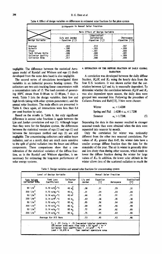
The first series of simulations investigated five vari- ables of a house heating system with a flat-plate collector. The five design variables, their low and high levels, and the annual solar fractions are given in Table 3. The main effects (i.e. the changes in the differences between the annual solar fractions resulting from changing the levels of the design variables) are given in Table 4; the inter- action effects are not given, as all were less than 0.4 per cent solar fraction.

The results in Table 4 indicate that the only significant difference in annual solar fractions is between the Liu and Jordan correlation and eqn (1). For the range of system parameters investigated, the effect of adding a statistical variance to eqn (I) on the simulation results is

Table 3. Design variables and annual solar fractions for flat plate system

Level of Design Variable Annual Solar Fraction

Collector Collector Tank Vo1~e Collector Gollector Llu and Equatlon Aerospace Statistical Azlmuth Slope ~ r e a Quality ArR ~rdan [I] Eq. [I]

35 l/m! "Poor" 45 .~ 35 1/m', "Good" 45 m 2 35 l/re' "Good" 45 m 2 35 1/m', "Poor" 45 m 2

150 l/m', "Good" 45 1/m',

ea 2 150 "Poor" 45 m 2 150 l/re' "Poor" 45 m 2 150 1/m', "Good" 45 m 2

35 1/m' "Good" 90 m 2 35 1/m', "Poor" 90 m 2 35 1/m', "Poor" 90 m 2 35 l/re' "Good" 90 m 2

150 I/m' "Poor" 90 m E 150 l/re', "GOod" 90 m 2 150 1/m', "Good" 90 m 150 1/m' "Poor" go m 2

.39 .37 .37 .37

.52 .48 .49 .49

.4S .41 .42 .43

.28 .26 .26 .26

.60 .55 .S6 .57

.40 .38 .38 .38

.36 .33 .33 .33

.4S .41 .41 .42

.72 .66 .67 .69

.4g .45 .46 .47

.44 .40 .41 .41

.57 .51 .52 .54

.S8 .54 .55 .55

.69 .64 .66 .66

.70 .63 .65 .65

.45 .41 .41 .42

Average for All Runs .Sl .46 .47 .48

Collector Type F' ~ a KL Ube (w/m 2 - °C) Covers

"Poor" .75 .95 .gS .06 1.4 single "Good" .g5 .lO .95 .012 .Z8 single

UAHous E - 333 w/m 2 - °C UTANK - .28 w/m 2 - °C MCOLLECTO R ° - 60 kg/m 2 - hr

298 D. G. ERBS et al.

Table 4. Effect of design variables on differences in estimated solar fractions for fiat plate system

DifferenCe in Annual Solar Fraction

Design Variable

Average Azlmuth Slope Tank Volume Ratio Collector Quality Collector Area

(Llu and Jordan - Equation [l])

.043 - . 005

.006

.006

.017

.017

Main Effect of Design Variable

(Statistical Correlation

-Equation [ l ] )

.014 -.003 -.001

• 000 .010 .008

(Aerospace -Equation [ l ] )

.007 -•004

• 000 • O01

-•004 • 006

negligible. The difference between the statistical Aero- space model of Randall and Whitson and eqn (1) (both developed from the same data base) is also negligible.

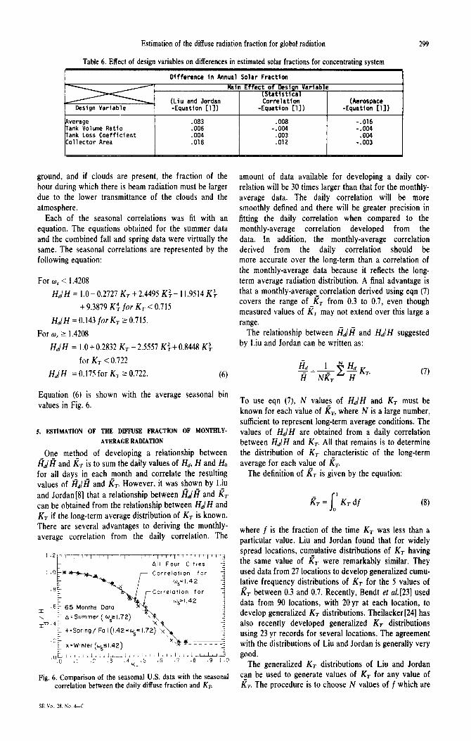
The second series of simulations investigated three variables in an industrial process heating system. The collectors are two-axis tracking linear concentrators with a concentration ratio of 15. The load consists of generat- ing 100°C steam from 8:00am to 12:00pm, 5 days a week. Table 5 lists the design variables, their low and high levels (along with other system parameters), and the annual solar fractions. The main effects are presented in Table 6. Once again, all interactions were less than 0.4 per cent fraction by solar.

Based on the results in Table 6, the only significant difference in annual solar fractions is again between the Liu and Jordan correlation and eqn (1). Although larger than they were for the flat-plate system, the differences between the statistical version of eqn (1) and eqn (1) and between the Aerospace method and eqn (1) are still negligible. The concentrating collectors only utilize beam radiation, and as a result, they are much more sensitive to the split of global radiation into the beam and diffuse components. These comparisons show that a con- sideration of the statistical variation of the diffuse frac- tion, as in the Randall and Whitson algorithm, is un- necessary for estimating the long-term performance of solar energy systems.

4• ESTIMATION OF THE DIFFUSE FRACTION OF DAILY GLOBAL RADIATION

A correlation was developed between the daily diffuse fraction, ttd/H, and KT using the hourly data from the four U.S. locations. It was shown earlier that the cor- relation between IJI and kr is seasonally dependent• To determine whether the correlation between HSH and g r was also dependent upon season, the daily data were grouped into seasonal bins. Following the procedure of Collares-Periera and Rabl[13], 3 bins were chosen:

Winter ~, < 1•4208

Spring and Fall 1.4208 -< cos -< 1.7208

Summer ~o, > 1.7208. (5)

Separating the data in this manner resulted in stronger seasonal trends than were obtained when the data were separated into seasons by month.

Only the correlation for winter was noticeably different from the other two seasonal correlations• For values of Kr greater than 0.45, the winter data have a smaller average diffuse fraction than the data for the remainder of the year• The air in winter is generally drier and less dusty than during other seasons, which tends to lower the diffuse fraction during the winter for large values of Kr. In addition, the lower solar altitude in the winter allows less of the scattered radiation to reach the

Table 5. Designvariables and annual solar fractions for concen~ating system

Level of Design Variable Annual Solar Fraction

Tank Vohm~ Tank L o s s Collector Llu and Equation Stetlstlca; Collector A rea Coefficient Area Jordan [ l ] Aerospace [ l ]

50 I/m 2 0.70 w/m~-°C 40 m~

200 I/m 2 0.70 w/m2-°C 40 m 2 50 I/m 2 0.14 ~/m~-% 40 m2

200 I/m 2 0.14 w/#-°C 40 m 2

50 I/m 2 0.70 w/m2-°C 80 m 2

200 I/m z 0.70 w/m2-°C 80 m 2

50 I/m 2 0.14 w/m2-°C 80 m 2

200 I/m 2 0.14 w/m2-°C 80 m 2

.38 •31 .29 •31

.31 .24 .23 •24

.44 .35 .33 .35

.43 .36 .35 •36

.65 .56 .54 .58

.58 . 4 9 . 4 6 .49

.72 .64 •62 .65

.75 .65 .63 .66

Average fo r Al l Runs .53 .45 .43 .46

F D = .B5 ( ~ ) n = •75 Evacuated tubular receivers C811ector area mass f low rate - SO kg/m~- hr * Col lector loss coe f f i c ien t - .13 w/m - C Load - 16,670 W *per nomtnal aperature area

Estimation of the diffuse radiation fraction for global radiation 299

Table 6. Effect of design variables on differences in estimated solar fractions for concentrating system

Design Variable

~verage Tank Volume Ratio Tank Loss Coefficient 3ollector Area

Difference in Annual Solar Fraction

(Liu and Jordan -Equation [l])

• 083 • 006 • 004 .018

Main E f fec t o f Design Var lab]e t S t a t l s t l c a l Corre la t ion

-Equation [ 1 ] )

• 0 0 8 - . 0 0 4

• 0 0 3 . 0 1 2

(Aerospace -Equation [ 1 ] )

-.016 - . 004

. 0 0 4 -•003

ground, and if clouds are present, the fraction of the hour during which there is beam radiation must be larger due to the lower transmittance of the clouds and the atmosphere•

Each of the seasonal correlations was fit with an equation. The equations obtained for the summer data and the combined fall and spring data were virtually the same. The seasonal correlations are represented by the following equation:

For o~s < 1.4208

HdlH = 1.0 - 0.2727 KT + 2.4495 K~-- 11.9514 K 3

+ 9.3879 K~ for Kr < 0.715

HJ H = 0.143 [or K~ >- 0.715.

For w, -> 1.4208

Hd/H = 1.0+0.2832 Kr -2.5557 K2+ 0.8448 K]-

for Kr < 0.722

Hd/H = 0.175 for K~ - 0.722. (6)

Equation (6) is shown with the average seasonal bin values in Fig. 6.

5. ESTIMATION OF THE DIFFUSE FRACTION OF MONTHLY-

AVERAGE RADIATION

One method of developing a relationship between ftd[~I and/~T is to sum the daily values of Hal, H and Ho for all days in each month and correlate the resulting values of/~u[/'t and/(T. However, it was shown by Liu and Jordan[8] that a relationship between ffIu[~I and/~T can be obtained from the relationship between HdlH and KT if the long-term average distribution of Kr is known. There are several advantages to deriving the monthly- average correlation from the daily correlation. The

~ - All Four Ci t ies -~ 1 . 0 ~ 1 ~ I ~ ¢ ~ . / -~ Cor re lo f ion fo r

F ' ~ . ~ / ~'s ̀-q'42 t 8F- \ 7 r -c°,re'°''°°'°r 1

b : "1~ 7 Cds>l'42

T'O'4 ~- + :Spr ing/Fo l l (I .42-~S-1.72) ~ x ~ .

• 2~ ~ x = Winter (WsSl.42) x.x_ ~ . . . . . .OL t <1, I LL ,~ , l l ~ , 1, ~, I , x ~ ! _ ~ I , i , I , i , I , i ~

• 0 . l .2 .3 .4 .5 .6 .7 .8 .9 l.O K T

Fig. 6. Comparison of the seasomal U.S. data with the seasonal correlation between the daily diffuse fraction and KT.

amount of data available for developing a daily cor- relation will be 30 times larger than that for the monthly- average data. The daily correlation will be more smoothly defined and there will be greater precision in fitting the daily correlation when compared to the monthly-average correlation developed from the data. In addition, the monthly-average correlation derived from the daily correlation should be more accurate over the long-term than a correlation of the monthly-average data because it reflects the long- term average radiation distribution. A final advantage is that a monthly-average correlation derived using eqn (7) covers the range of /~r from 0.3 to 0.7, even though measured values o f / ( r may not extend over this large a range.

The relationship between ~Id]lTt and Hd/H suggested by Liu and Jordan can be written as:

- ~ : NRT -~ Kr. (7)

To use eqn (7), N values of HdIH and Kr must be known for each value of/(St, where N is a large number, sufficient to represent long-term average conditions. The values of HJH are obtained from a daily correlation between HalH and Kr. All that remains is to determine the distribution of Kr characteristic of the long-term average for each value of/(T.

The definition of/~T is given by the equation:

1

Rr = KT df (8)

where jr is the fraction of the time Kr was less than a particular value. Liu and Jordan found that for widely spread locations, cumulative distributions of Kr having the same value of /(r were remarkably similar. They used data from 27 locations to develop generalized cumu- lative frequency distributions of Kr for the 5 values of /~r between 0.3 and 0.7. Recently, Bendt et al. [23] used data from 90 locations, with 20 yr at each location, to develop generalized KT distributions. Theilacker [2.4] has also recently developed generalized Kr distributions using 23 yr records for several locations. The agreement with the distributions of Liu and Jordan is generally very good.

The generalized Kr distributions of Liu and Jordan can be used to generate values of Kr for any value of /(T. The procedure is to choose N values of f which are

SE VoL 28, No. 4--C

300

equally spaced between 0 and 1. The corresponding values of Kr are then found from the appropriate /~'r curve. This allows eqn (7) to be evaluated for values of /~r between 0.3 and 0.7. The seasonal daily diffuse correlation, eqn (6), was used along with eqn (7) and the Kr distributions of Liu and Jordan as curve fit by Cole[25] to derive a seasonal monthly-average daily diffuse correlation. The following equation was fit to the correlation:

For co, -< 1.4208 and 0.3 - /~T -< 0.8

#,d/Y = 1.391 - 3.560/~r + 4.189 g~-- 2.137/~]-

For o~, > 1.4208 and 0.3 -</~r -< 0.8

HJH = 1.311 - 3.022/~r + 3.427/C]-- 1.821/~']-.

D. G. ERBS et aL

moisture and dust content of the air and in the dis- tribution of cloud cover. The hourly data for the four U.S. locations were also used to develop a nonseasonal daily diffuse correlation from which the following non- seasonal monthly-average daily diffuse correlation was derived:

For 0.3 -</~r -< 0.8

fta[tt = !.317 - 3.023/~r + 3.372/Cr - 1.769/C~. (10)

(9)

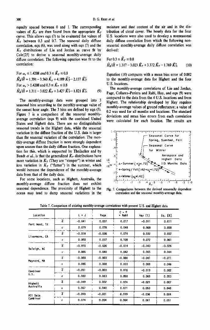
The monthly-average data were grouped into 3 seasonal bins according to the monthly-average value of the sunset hour angle. The 3 bins are defined by eqn (5). Figure 7 is a comparison of the seasonal monthly- average correlation (eqn 9) with the combined United States and Highett data. There are no distinguishable seasonal trends in the Highett data, while the seasonal variation in the diffuse fraction of the U.S. data is larger than the seasonal variation of the correlation. The mon- thly-average diffuse fraction is more strongly dependent upon season than the daily diffuse fraction. One explana- tion for this, which is supported by Theilacker and by Bendt et aL, is that the generalized Kr distributions have more variation in Kr (They are "steeper") in winter and less variation in Kr ("flatter") in the summer, which would increase the dependence of the monthly-average data from that of the daily data.

For some locations, such as Highett, Australia, the monthly-average diffuse fraction does not exhibit seasonal dependence. The proximity of Highett to the ocean may tend to damp seasonal variations in the

Equation (10) compares with a mean bias error of 0.002 to the monthly-average data for Highett and the four U.S. locations.

The monthly-average correlations of Liu and Jordan, Page, Collares-Periera and Rabl, Hay, and eqn (9) were compared to the data from the 4 U.S. locations and from Highett. The relationship developed by Hay requires monthly-average values of ground reflectance; a value of 0.2 was used for all months and locations. The standard deviations and mean bias errors from each correlation were calculated for each location. The results are

l " 2 ~ - ' l ' l ' l ' l ' l ' l ' r ' l ' r' I ' l ' l ' ~ ' r ' l ' r ' ' ' i ' ' I I " O E . 8~-;.~ ~- \1(///~/ Spring, Summer, F a l l f i - - SeasonaIseasonalfor WinterCUrVecurve for

.6~- \ " ~ Aerospace and I I L- "~ ~'~-~ Highett Data 1

.4~zx-Sumrner(OJs~l.7~')"~'~ll3 Months Data ,1 l ie • 2 1 +-Spring/Fall (l.42 ~wsc 1.72)>t'~q- ~'~.....

~- x=Winter (%-1.42) "~ O F , J , ] , * , I , l , l , ~ , I L I L J , I , I , I , I , I , I , J , l , I • 0 .1 .2 .3 .4 ~.T. 5 .6 .7 .8 .9 1.0

Fig. 7. Comparisons between the derived seasonally dependent correlation and the seasonal monthly-average data.

Table 7. Comparison of existing monthly-average correlations with present U.S. and Highett data

Location

Fort Hood, TX

Livermore, CA

Raleigh, NC

~aynard, MA

Combined U.S.

Highett ~ustralia

M1 Data Combined

o

o

o

c7

C-P L + J Page + Rabl Hay (I) Eq. [8]

-0.041 0.007 0.017 -0.011 0.011

0.079 0.078 0.048 0.068 0.058

-0.018 -0.008 0.076 0.032 0.032

0.058 0.037 0.109 0.072 0.061

-0.070 -0.026 -0.014 -0.043 -0.026

0.085 0.048 0,042 0.065 0.044 -0.069 -0.003 -0.000 -0.041 -O.Oll

0.086 0.058 0,033 0.068 0.046 -0.051 -0.003 0.016 -O.01g 0.002

0.080 0.063 0.058 0.068 0.053 -0.049 0.002 0.024 -0.021 0.007

0.067 0.040 0.071 0.050 0.048

-0.050 -0.001 0.019 -0.036 0.004 0.074 0.054 0.064 0.061 0.051

Extimation of the diffuse radiation fraction for global radiation

presented in Table 7. The Liu and Jordan correlation and a absorptance eqn (9) were derived from daily correlations, while the ~ emittance other relationships were developed using monthly- p coefficient ofautocorrelation average data. cr standard deviation

~- transmittance ~, sunset hour angle

6. CONCLUSIONS

The correlation developed between the hourly diffuse fraction and kr was found to be essentially the same as the relationship previously developed by Orgiil and Hollands [2], although different data were used in each case. Data recorded in Highett, Australia were also found to agree to within a few per cent with the hourly relationship presented. While the uncertainty in the estimated diffuse fraction for an hour is significant, the correlation predicts the long-term average hourly diffuse fraction accurately. For the systems investigated, the importance of simulating the distribution of hourly diffuse fractions about the long-term average in com- puter simulations is minor. Only the long-term relation- ship between Id]I and kr, and not the random nature of Id/I, appears to be important. For simulations involving a flat-plate collector system, the results obtained with different correlations were generally within 5 per cent of each other, but for a concentrating collector system, the Liu and Jordan daily diffuse correlation resulted in significantly higher estimates of system performance. The seasonal monthly-average daily diffuse correlation given by eqn (9), which was derived from a seasonal daily diffuse correlation, agrees closely with the monthly- average U.S. and Highett data. The monthly-average correlations of Collares-Pereira and Rabl and of Page agree with the U.S. and Highett data nearly as well as the monthly-average correlations presented.

NOMENCLATURE

a diffuse fraction residual d bias error d mean bias error / cumulative fraction of occurrence 3~ annual solar fraction F' collector efficiency factor F~ collector heat removal factor H daily total radiation incident on a horizontal surface

Ha daily diffuse radiation incident on a horizontal surface Ho daily extraterrestrial radiation incident on a horizontal sur-

face monthly-average daily total radiation incident on a

horizontal surface Hd monthly-average daily diffuse radiation incident on a

horizontal surface Ho monthly-average daily extraterrestrial radiation incident on

a horizontal surface I hourly total radiation incident on a horizontal surface

/~ hourly "clear sky" total radiation incident on a horizontal surface

ld hourly diffuse radiation incident on a horizontal surface Io hourly extraterrestrial radiation incident on a horizontal

surface K extinction coefficient kc hourly clearness index (ratio of I to Ic) kr hourly clearness index (ratio of I to I0)

K r daily clearness index (ratio of H to Ho) Kr monthly-average daily clearness index (ratio of/~ to Ho)

L length, thickness N number of days U loss coefficient

Subscripts b back c calculated e edge

m measured n normal

301

REFERENCES

I. E. C. Boes, Estimating the direct component of solar radia- tion. Sandia Report SAND75-0565, (1975).

2. J. F. Orgill and K. G. T. Hollands, Correlation equation for hourly diffuse radiation on a horizontal surface. Solar Energy 19, 357 (1977).

3. R. Bruno, A correction procedure for separating direct and diffuse insolation on a horizontal surface. Solar Energy 20, 97 (1978).

4. J. W. Bugler, The determination of hourly insolation on an inclined plane using a diffuse irradiance model based on hourly measured global horizontal insolation. Solar Energy 19, 477 (1977).

5. J. A. Duffie and W. A. Beckman, Solar Engineering of Thermal Processes. Wiley New York (1980).

6. C. M. Randall and M. E. Whitson, Final report--hourly insolation and meteorological data bases including improved direct insolation estimates. Aerospace Report No. ATR-78 (7592)-1 (1977).

7. SOLMET, Volume 2--Final report Hourly solar radiation surface meterological observations. TD--9724 (1979).

8. B. Y. H. Liu and R. C. Jordan, The interrelationship and characteristic distribution of direct, diffuse, and total solar radiation. Solar Energy 4, 1 (1960).

9. N. K. D. Choudhury, Solar radiation at New Delhi. Solar Energy 7, 44 (1963).

10. G. Stanhlll, Diffuse sky and cloud radiation in Israel. Solar Energy 19, 96 (1966).

11. S. E. Tuller, The relationship between diffuse total, and extra terrestrial solar radiation. Solar Energy IS, 259 (1976).

12. D. W. Ruth and R. E. Chant, The relationship of diffuse radiation to total radiation in Canada. Solar Energy 18, 153 (1976).

13. M. Collares-Pereira and A. Rabl, The average distribution of solar radiation---correlations between diffuse and hemis- pherical and between daily and hourly insolation values. Solar Energy 22, 155 (1979).

14. J. K. Page, The estimation of monthly mean values of daily total short-wave radiation on vertical and inclined surfaces from sunshine records for latitudes 400N---40"S. Proc. UN Conference on New Sources of Energy 4, 378 (1964).

15. M. Iqbal, A study of Canadian diffuse and total solar radiation data--I. Monthly average daily horizontal radiation, Solar Energy 22, 81 (1979).

16. J. E. Hay, Calculation of monthly mean solar radiation for horizontal and inclined surfaces. Solar Energy 23, 301 (1979).

17. J. W. Bannister, Solar radiation records. Division of Mechanical Engineering, Commonwealth Scientific and In- dustrial Research Organization, Highett, Victoria, Australia (1966--69).

18. Monthly solar climatological summary for the solar energy meteorological research and training site--region 2. Atmos- pheric Sciences Research Center, State University of New York at Albany, Albany, New York (1980).

19. H. C. Hottel, A simple model for estimating the trans- mittance of direct solar radiation through clear atmosphere. Solar Energy 18, 129 (1976).

20. G. E. P. Box and G. M. Jenkins, Time Series Analysis Forecasting and Control. Holden-Day, San Francisco (1970).

302 D. G. ERBS et aL

21. S. A. Klein et al. 'TRNSYS--transient simulation program. University of Wisconsin-Madison Engineering Experiment Station Report 38-10, Version 10.1 (1979).

22. G. E. P. Box, W. G. Hunter and J. S. Hunter, Statistics for Experimenters Wiley New York (1978).

23. P. Bendt, A. Rabl and M. Collares-Pereira, the frequency distribution of daily isolation values. Solar Energy Research Institute, Submitted to Solar Energy (1980).

24. J. C. Theilacker, An investigation of the monthly-average utilizability for flat-plate solar collectors. Masters Thesis in Mechanical Engineering, University of Wisconsin-Madison (19S0).

25. R. J. Cole, Long-term average performance predictions for CPC's Proc. Am. Section of I.S.E.S., Orlando, Florida (1977).