Embed Size (px)
Citation preview
İstatistikçiler Dergisi: İstatistik & Aktüerya
Journal of Statisticians: Statistics and Actuarial Sciences
IDIA 9, 2016, 2, 79-86
Geliş/Received:15.08.2016, Kabul/Accepted: 16.12.2016
www.istatistikciler.org
Araştırma Makalesi / Research Article
Estimation of sample size and power
for general full factorial designs
Melike Kaya Bahçecitapar
Hacettepe University
Faculty of Science
Department of Statistics
06800-Beytepe, Ankara, Turkey
Özge Karadağ
Hacettepe University
Faculty of Science
Department of Statistics
06800-Beytepe, Ankara, Turkey
Serpil Aktaş
Hacettepe University
Faculty of Science
Department of Statistics
06800-Beytepe, Ankara, Turkey
Abstract
The aim of this study is to calculate sample size and power for several varieties of general full factorial
designs, in order to help researchers to avoid the waste of resources by collecting surplus data before
designing experiments. It was found out that the calculations were significantly affected by many factors in
full factorial experimental designs, such as number of levels for each factor, number of replications,
maximum difference between main effect means and standard deviation.
Keywords: full factorial design, statistical power, sample size, power of test
Öz
Genel tam faktöriyel deney tasarımlarda örneklem büyüklüğü ve güç tahmini
Bu çalışmanın amacı, farklı boyutlardaki çok sayıda genel tam faktöriyel tasarımlar için örneklem
büyüklüğü ve güç hesaplamalarıni yaparak, deney tasarımını kurmadan önce gereğinden fazla veri
toplamanın neden olduğu kaynak israfını önlemektir. Bu hesaplamaların faktörlerin düzey sayısı, analizde
kullanılan modeldeki ana etkilerin ortalamaları ve standart sapma gibi birçok faktöre dayalı olduğu
görülmüştür.
Anahtar sözcükler: tam faktöriyel tasarım, istatistiksel güç, örneklem büyüklüğü, testin gücü
1. Introduction
Full factorial design approaches are the most commonly utilized ways to carry out experiments with two
or more factors. These designs allow researcher workers to analyze responses (i.e. observations) measured
at all combinations of the experimental factor levels. In many applied research work, full factorial designs
are used to answer questions such as: i) which factors have the most influence on the response, and ii) are
M. Kaya Bahçecitapar, Ö. Karadağ, S. Aktaş / İstatistikçiler Dergisi: İstatistik&Aktüerya, 2016, 9, 79-86
80
there any interactions between two or more factors that influence the response? For instance, in
educational studies, the researchers often use factorial designs to assess educational methods taking into
account the influence of socio-economic, demographic or related factors. Lodico et al.[1] analyzed the
reaction problem of boys and girls to computer use, and whether this reaction can influence their math
achievement by using a factorial design. Hereby, educational researchers are interested in
determining the effectiveness of certain techniques in classroom teaching. Similarly, by examining the
multiple variables we get more accurate results of other real life examples.
The simplest type of factorial designs involves only two factors each including two levels, which is
usually called a factorial design. In factorial designs, a total of combinations
exist and thus, four runs are required for an experiment without replicate. Replicate is the number of times
a treatment combination is run. A general full factorial design is used when any experimental factor has
more than two levels with or without replicate. For general full factorial designs, ANOVA shows which
factors are significant and regression analysis provides the coefficients for the prediction equations.
If the number of factors, level of factors and replicate of the experiment are too high, the most costly
experimental resources are encountered. The fact that the sample size grows in the number of factors and
levels of factors makes full factorial designs too expensive to run for the purpose of experiment. For this
reason, after defining the research question and relevant hypotheses for the experimental design to be
attempted, how many numbers of factors, levels of factors and replication of each combination will be
included, namely estimation of the sample size is an important consideration in designing the experiment.
Browner et. al. [2] suggested some strategies to minimize the sample size through power analysis.
Statistical power calculation is one of the methods in sample size estimation, which can be estimated
before collecting necessary data set for the study. In factorial designs, power is generally used to ensure
that the hypothesis test will detect significant effects (or differences). However, in a full factorial
designed experiment, there are many factors affecting power calculation: such as number of levels,
standard deviation of responses, number of replicates and maximum difference between main effect
means.
In this paper, we examine sample size and power calculations for several varieties of general full factorial
designed experiments with different numbers of levels of factors and replicates under different values of
maximum difference between main effect means. Thus we indicate the calculation of sample size through
power analysis in order to avoid unnecessary levels of factors and number of replications that might cause
waste of time and resources in the experimental designs, and hence to analyze responses out of as few
runs as possible in several full factorial designs.
2. General factorial designs
Factorial designs have been widely used in manufacturing industry studies as a tool of maximizing output
(response) for the given input factors [3-5]. The simplest full factorial design may be extended to
the 2-factor factorial design with levels a for factor A, levels b for factor B and n replicates, or general full
factorial designs with k-factors including 2 or more than 2 levels and n replicates. For general full
factorial design with k-factors, each factor with any number of levels, the model is sum of means of all
observations, k main effects, two-factor interactions, three-factor interactions, …etc., until k-
factor interaction and error term (if n> 1).
The observations in a factorial experiment with three factors A, B, C at levels a, b, c and n replicates are
shown in Table 1. In this kind of experiment, total observations will be . They can be
described by a model in Eq. (1) [6]:
(1)

M. Kaya Bahçecitapar, Ö. Karadağ, S. Aktaş / İstatistikçiler Dergisi: İstatistik&Aktüerya, 2016, 9, 79-86
81
i= ; ; ;
where, is a response in l’th replicate with factors A, B, C at levels i, j, k, respectively; is the overall
mean effect; , and are main effects of factors A,B, C at levels i, j, k, respectively; is the effect
of the interaction between
and , is the effect of the interaction between and ; is the
effect of the interaction between and ; is the effect of the three-factor interaction between ,
and and finally is a random error component.
Table 1. Representation of three-factor factorial designs with n replicates
In a factorial experiment with factor A at a levels and factor B at b levels, the fixed-effects model is also
described as
, (2)
where is a response in n replicate with factors A and B at levels i and j respectively; is the overall
mean effect; and are main effects of factors A and B at levels i and j respectively; is the effect
of the interaction between
and and represents the error term.
The two-way analysis of variance (two-way ANOVA) is the most popular layout in the design of
experiments with two factors. When the factorial experiment is conducted with an equal number of
replicate per factor-level combination, computational formula and analysis summary for two-way
ANOVA are given in Table 2.
Table 2. The general case for two-way ANOVA
Source of
variation
Sum of squares
(SS)
Degrees of
freedom
(df)
Mean square
(MS) F-statistic
Rows (A) 2
A .. ...
=1
SS =a
i
i
nb Y Y a-1 A ASS /df A ErrorMS MS
Columns (B) 2
B . . ...
1
SS =b
j
j
n a Y Y
b-1 B BSS /df B ErrorMS MS
Factor B
1 2 b
Factor C Factor C Factor C
1 2 c 1 2 c 1 2 c
F
act
or
A
1
Y1111
Y1112
…
Y111n
Y1121
Y1122
…
Y112n
Y11c1
Y11c2
…
Y11cn
Y1211
Y1212
…
Y121n
Y1221
Y1222
…
Y122n
Y12c1
Y12c2
…
Y12cn
Y1b11
Y1b12
…
Y1b1n
Y1b21
Y1b22
…
Y1b2n
Y1bc1
Y1bc2
…
Y1bcn
a
Ya111
Ya112
…
Ya11n
Ya121
Ya122
…
Ya12n
Ya1c1
Ya1c2
…
Ya1cn
Ya211
Ya212
…
Ya21n
Ya221
Ya222
…
Ya22n
Ya2c1
Ya2c2
…
Ya2cn
Yab11
Yab12
…
Yab1n
Yab11
Yab12
…
Yab1n
Yabc1
Yabc2
…
Yabcn

M. Kaya Bahçecitapar, Ö. Karadağ, S. Aktaş / İstatistikçiler Dergisi: İstatistik&Aktüerya, 2016, 9, 79-86
82
Interaction (AB) 2
AB . .. . .
=1 =1
SS = ...b a
ij i j
j i
n Y Y Y Y (a-1)(b-1) AB ABSS /df AB ErrorMS MS
Error 2
Error .
=1 =1 =1
SS =n a b
ijk ij
k i j
Y Y ab(n-1) Error ErrorSS /df
Total 2
Total ...
=1 =1 1
SS =n a b
ijk
k i j
Y Y
abn-1
The following hypothesis tests are used to check whether each of the factors in two factorial design is
significant or not:
vs. at least one
vs. at least one
i, j vs. at least one
The F- test statistics for these three tests are given in Table 2. They are identical with the partial F-test in
multiple linear regression analysis.
3. Power and sample size estimation in factorial designs
In full factorial designs, statistical power depends on the following parameters: i) standard deviation (to
indicate experimental variability), ii) maximum difference between main effect means, iii) number of
replicates, iv) number of levels for factors in the model and v) the significance level (i.e., the Type I error
probability). Cohen [7] suggested and classified the effect sizes as “small,” “medium,” or “large”. Effect
sizes of interest may vary according to the essence of the research work under concern.
The power of an experiment is the probability of detecting the specified effect size. A power analysis can
be used to estimate the sample size that would be needed to detect the differences involved. Power and
sample size calculations should be considered in the design phase of any research study to avoid choosing
a sample size that might be too large and costly or too small and possibly of inadequate sensitivity.
Therefore, in planning and development stage of experimental designs, a sample size calculation is a
critical step. In most studies, sample size calculation requires to maintain a specific statistical power (i.e.,
e.g. 80 % power).
In factorial designs, except the levels of factors, the number of replicates or observations taken from each
case in design forwards a sample size for factorial designs. The engineer or investigator wishes to decide
how many replicates should be taken and the number of replicates, which is suitable for the desired
power. For this purpose, we give some tables which include the number of replicates, values of power
according to the properties of general full factorial design (standard deviation, levels of factors and values
of the maximum difference between main effect means).
When the true difference between the means is , suppose the desired power (i.e., the chance of finding a
significant difference) is . Let denote the standard normal curve value cutting off the proportion
β in the upper tail. For example, if 95% power is demanded, = 0.95 so that β = 0.05 and =
1.645.The sample size for any study depends on the i) acceptable level of significance, ii) power of the
study, iii) expected effect size and iv) standard deviation in the population [8, 9].
In this study, MINITAB 17 statistical software program was performed for sample size and power
calculations of several general factorial designs as in the study of Kirby et al. [8]. Calculations for
factorial designs are implemented for the following parameters:

M. Kaya Bahçecitapar, Ö. Karadağ, S. Aktaş / İstatistikçiler Dergisi: İstatistik&Aktüerya, 2016, 9, 79-86
83
: 1, 1.5, 2 , 3 , 4
Number of replicates: 2,3,4
Dimension: 2x2x3, 3x3x2, 3x3x3, 3x3x4, 4x4x2
Mean difference: 2, 2.5, 3
Table 3 gives the power calculations under those various combinations. The power in Table 3 may be a
guide for determining the sample size. The other combinations might be studied to calculate the sample
size for a different combination of levels of , number of replications, dimension and mean difference.
Table 3. Power calculations for general full factorial design under different conditions
a×b×c
2×2×3 3×3×2 3×3×3 3×3×3 4×4×2
σ Number
of
replicates
Mean difference Mean difference Mean difference Mean difference Mean difference
2 2.5 3 2 2.5 3 2 2.5 3 2 2.5 3 2 2.5 3
2 0.89 0.98 0.99 0.98 0.99 0.99 0.99 1 1 0.99 1 1 0.85 0.97 0.99
1 3 0.98 0.99 1 0.99 1 1 1 1 1 1 1 1 0.98 0.99 0.99
4 0.99 1 1 0.99 1 1 1 1 1 1 1 1 0.99 0.99 1
2 0.55 0.75 0.89 0.77 0.99 0.99 0.93 0.99 0.99 0.90 0.98 0.99 0.49 0.69 0.85
1.5 3 0.79 0.94 0.98 0.94 0.99 0.99 0.99 0.99 1 0.98 0.99 1 0.73 0.91 0.98
4 0.91 0.98 0.99 0.99 0.99 0.99 0.99 1 1 0.99 0.99 1 0.87 0.97 0.99
2 0.33 0.49 0.65 0.51 0.71 0.86 0.72 0.89 0.97 0.45 0.66 0.82 0.28 0.43 0.59
2 3 0.53 0.73 0.87 0.73 0.91 0.98 0.90 0.98 0.99 0.66 0.86 0.96 0.47 0.67 0.84
4 0.68 0.86 0.96 0.86 0.97 0.99 0.97 0.99 0.99 0.81 0.95 0.99 0.61 0.82 0.94
2 0.17 0.24 0.33 0.25 0.37 0.51 0.38 0.55 0.72 0.32 0.48 0.66 0.14 0.21 0.29
3 3 0.26 0.38 0.53 0.39 0.56 0.73 0.56 0.76 0.90 0.49 0.70 0.86 0.22 0.33 0.47
4 0.35 0.52 0.69 0.51 0.71 0.86 0.70 0.88 0.96 0.64 0.84 0.95 0.29 0.45 0.62
2 0.12 0.15 0.21 0.16 0.23 0.31 0.23 0.34 0.46 0.19 0.29 0.40 0.11 0.13 0.17
4 3 0.16 0.23 0.32 0.23 0.34 0.47 0.34 0.50 0.67 0.29 0.44 0.60 0.14 0.20 0.27
4 0.21 0.31 0.43 0.31 0.45 0.61 0.44 0.64 0.80 0.39 0.57 0.75 0.18 0.26 0.37
With the fixed values of and number of replicates, if the maximum difference between means increases,
the power increases. For each general full factorial design with fixed main difference and value, if the
number of replicates increases, the power increases.
Table 4 presents power calculations for factorial designs for different values of maximum
difference and number of replications. Estimation of sample size is illustrated for power=0.90 and
standard deviation=1. It is seen that the highest actual power is obtained for the dimension with 32
total runs and number of replications=2.
Table 4. Estimation of sample size for power=0.90 and standard deviation=1
Maximum difference Number of dimensions Number of replication Actual power
1 2x2 12 0.92
2 2x2 4 0.96
2.5 2x2 3 0.96
1 3x3 9 0.91
2 3x3 3 0.95
2.5 3x3 2 0.91
1 2x3 14 0.92
2 2x3 4 0.92
2.5 2x3 3 0.93
1 4x4 8 0.93
2 4x4 3 0.98
2.5 4x4 2 0.97
M. Kaya Bahçecitapar, Ö. Karadağ, S. Aktaş / İstatistikçiler Dergisi: İstatistik&Aktüerya, 2016, 9, 79-86
84
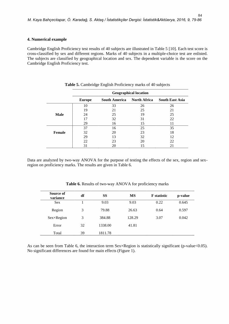
4. Numerical example
Cambridge English Proficiency test results of 40 subjects are illustrated in Table 5 [10]. Each test score is
cross-classified by sex and different regions. Marks of 40 subjects in a multiple-choice test are enlisted.
The subjects are classified by geographical location and sex. The dependent variable is the score on the
Cambridge English Proficiency test.
Table 5. Cambridge English Proficiency marks of 40 subjects
Geographical location
Europe South America North Africa South East Asia
10 33 26 26
19 21 25 21
Male 24 25 19 25
17 32 31 22
29 16 15 11
37 16 25 35
Female 32 20 23 18
29 13 32 12
22 23 20 22
31 20 15 21
Data are analyzed by two-way ANOVA for the purpose of testing the effects of the sex, region and sex-
region on proficiency marks. The results are given in Table 6.
Table 6. Results of two-way ANOVA for proficiency marks
Source of
variance df SS MS F statistic p-value
Sex 1 9.03 9.03 0.22 0.645
Region 3 79.88 26.63 0.64 0.597
Sex×Region 3 384.88 128.29 3.07 0.042
Error 32 1338.00 41.81
Total 39 1811.78
As can be seen from Table 6, the interaction term Sex×Region is statistically significant (p-value<0.05).
No significant differences are found for main effects (Figure 1).

M. Kaya Bahçecitapar, Ö. Karadağ, S. Aktaş / İstatistikçiler Dergisi: İstatistik&Aktüerya, 2016, 9, 79-86
85
male
female
25
24
23
22
21
South Ea
st A
sia
South Am
erica
North Af
rica
Euro
pe
Sex
Me
an
Region
Main Effects PlotFitted Means
Figure 1. Main effects plot for Cambridge English Proficiency marks
2,52,01,51,00,50,0
1,0
0,8
0,6
0,4
0,2
0,0
Maximum Difference
Po
we
r
A lpha 0,05
StDev 2
# Factors 2
# Lev els 2; 4
Blocks No
Term O rder 2
Terms Included In Model
A ssumptions
Figure 2. Power curve for general full factorial of Table 5
Figure 2 displays the power curve of this study. It is estimated approximately 80% based on alpha=5%,
standard deviation=2 and maximum difference=2.
5. Conclusion
Experimental design is the process of planning an experiment that collects the sufficient data to answer a
question of interest. Power of a test is the probability of detecting a true underlying difference. In this
study, we intend to find out the ideal number of replicates for various full factorial designs by
assigning some values to standard deviation ( ) of collected data and main difference. As the standard
deviation of collected data increases, power will decrease. For the large values of maximum differences,
power will increase in cases of included terms in the model up through order three and without including
blocks in the model. The main disadvantage of full factorial designs is the difficulty of experimenting
with more than two factors, or at many levels. Therefore, simplifying the factorial design process enables
the researchers a cost-effective process. MINITAB provides a simple and user-friendly method to
calculate power for full factorial designs. In the educational experiments, what sample is needed for the
M. Kaya Bahçecitapar, Ö. Karadağ, S. Aktaş / İstatistikçiler Dergisi: İstatistik&Aktüerya, 2016, 9, 79-86
86
experiment and sample size calculation is the first step of planning the experiment. It should carefully be
taken into consideration, that determining the sample size is very much related to research components
such as time and cost.
References
[1] M.D. Lodico, D.T. Spaulding, K.H. Voegtle, 2010, Methods in Educational Research:From Theory to
Practice, John Wiley&Sons.
[2] W.S. Browner, T.B. Newman, S.R. Cummings, S.B. Hulley, 2001, Estimating sample size and power: the
nity-gritty. In: Hulley, S.B., Cummings, S.R., Browner, W.S., Grady, D. , Hearst, N., Newman, T.B.
(editors). Designing clinical research: an epidemiologic approach. 2nd ed. Baltimore: Ed. Williams &
Wilkins; 65-91.
[3] P. Mathews, 2010, Sample Size Calculations: Practical Methods for Engineers and Scientists. Harbor, OH:
Mathews Malnar and Bailey, Inc.
[4] W. W. Daniel, C.L. Cross, 1999, Biostatistics: A foundation for analysis in the health sciences, 7th ed. New
York, NY: Wiley.
[5] G.E. Box, W.G. Hunter, J.S. Hunter, 2005, Statistics for Experimenters: Design, Innovation and Discovery,
2nd ed., Wiley.
[6] D.C. Montgomery, 2013, Design and Analysis of Experiments. 8th ed. New York: John Wiley & Sons, Inc.
[7] J. Cohen, 1988, Statistical Power Analysis for the Behavioral Sciences. 2nd ed. Mahwah NJ:Lawrence
Erlbaum Associates.
[8] A. Kirby, V. Gebski, A.C. Keech., 2002, Determining the sample size in a clinical trial. Med J Aust. 177
(5):256–7.
[9] Minitab 17 Statistical Software, 2010, State College, PA: Minitab, Inc. (www.minitab.com).
[10] D.R. Cox, 1958, Planning Experiments. New York: John Wiley & Sons, Inc.