Embed Size (px)
Citation preview
HELSINKI UNIVERSITY OF TECHNOLOGY
Department of Electrical and Communications Engineering
Laboratory of Acoustics and Audio Signal Processing
Sampo Vesa
Estimation of Reverberation Time from Binaural
Signals Without Using Controlled Excitation
Master’s Thesis submitted in partial fulfillment of the requirements for the degree of
Master of Science in Technology.
Espoo, October 8, 2004
Supervisor: Professor Matti Karjalainen
Instructors: D.Sc. (Tech.) Aki Härmä
HELSINKI UNIVERSITY ABSTRACT OF THE
OF TECHNOLOGY MASTER’S THESIS
Author: Sampo Vesa
Name of the thesis: Estimation of Reverberation Time from Binaural Signals
Without Using Controlled Excitation
Date: October 8, 2004 Number of pages: 100
Department: Electrical and Communications Engineering
Professorship: S-89
Supervisor: Prof. Matti Karjalainen
Instructors: D.Sc. (Tech) Aki Härmä
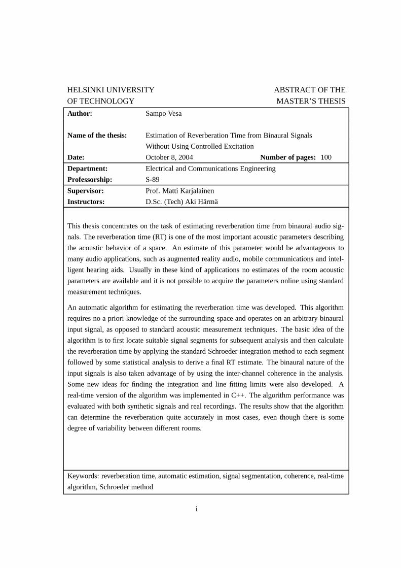
This thesis concentrates on the task of estimating reverberation time from binaural audio sig-
nals. The reverberation time (RT) is one of the most important acoustic parameters describing
the acoustic behavior of a space. An estimate of this parameter would be advantageous to
many audio applications, such as augmented reality audio, mobile communications and intel-
ligent hearing aids. Usually in these kind of applications no estimates of the room acoustic
parameters are available and it is not possible to acquire the parameters online using standard
measurement techniques.
An automatic algorithm for estimating the reverberation time was developed. This algorithm
requires no a priori knowledge of the surrounding space and operates on an arbitrary binaural
input signal, as opposed to standard acoustic measurement techniques. The basic idea of the
algorithm is to first locate suitable signal segments for subsequent analysis and then calculate
the reverberation time by applying the standard Schroeder integration method to each segment
followed by some statistical analysis to derive a final RT estimate. The binaural nature of the
input signals is also taken advantage of by using the inter-channel coherence in the analysis.
Some new ideas for finding the integration and line fitting limits were also developed. A
real-time version of the algorithm was implemented in C++. The algorithm performance was
evaluated with both synthetic signals and real recordings. The results show that the algorithm
can determine the reverberation quite accurately in most cases, even though there is some
degree of variability between different rooms.
Keywords: reverberation time, automatic estimation, signal segmentation, coherence, real-time
algorithm, Schroeder method
i
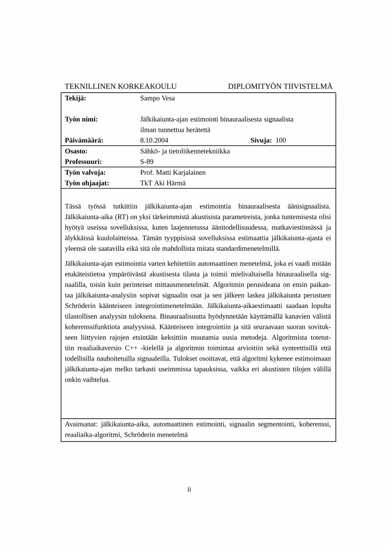
TEKNILLINEN KORKEAKOULU DIPLOMITYÖN TIIVISTELMÄ
Tekijä: Sampo Vesa
Työn nimi: Jälkikaiunta-ajan estimointi binauraalisesta signaalista
ilman tunnettua herätettä
Päivämäärä: 8.10.2004 Sivuja: 100
Osasto: Sähkö- ja tietoliikennetekniikka
Professuuri: S-89
Työn valvoja: Prof. Matti Karjalainen
Työn ohjaajat: TkT Aki Härmä
Tässä työssä tutkittiin jälkikaiunta-ajan estimointia binauraalisesta äänisignaalista.
Jälkikaiunta-aika (RT) on yksi tärkeimmistä akustisista parametreista, jonka tuntemisesta olisi
hyötyä useissa sovelluksissa, kuten laajennetussa äänitodellisuudessa, matkaviestinnässä ja
älykkäissä kuulolaitteissa. Tämän tyyppisissä sovelluksissa estimaattia jälkikaiunta-ajasta ei
yleensä ole saatavilla eikä sitä ole mahdollista mitata standardimenetelmillä.
Jälkikaiunta-ajan estimointia varten kehitettiin automaattinen menetelmä, joka ei vaadi mitään
etukäteistietoa ympäröivästä akustisesta tilasta ja toimii mielivaltaisella binauraalisella sig-
naalilla, toisin kuin perinteiset mittausmenetelmät. Algoritmin perusideana on ensin paikan-
taa jälkikaiunta-analysiin sopivat signaalin osat ja sen jälkeen laskea jälkikaiunta perustuen
Schröderin käänteiseen integrointimenetelmään. Jälkikaiunta-aikaestimaatti saadaan lopulta
tilastollisen analyysin tuloksena. Binauraalisuutta hyödynnetään käyttämällä kanavien välistä
koherenssifunktiota analyysissä. Käänteiseen integrointiin ja sitä seuraavaan suoran sovituk-
seen liittyvien rajojen etsintään keksittiin muutamia uusia metodeja. Algoritmista totetut-
tiin reaaliaikaversio C++ -kielellä ja algoritmin toimintaa arvioitiin sekä synteettisillä että
todellisilla nauhoitetuilla signaaleilla. Tulokset osoittavat, että algoritmi kykenee estimoimaan
jälkikaiunta-ajan melko tarkasti useimmissa tapauksissa, vaikka eri akustisten tilojen välillä
onkin vaihtelua.
Avainsanat: jälkikaiunta-aika, automaattinen estimointi, signaalin segmentointi, koherenssi,
reaaliaika-algoritmi, Schröderin menetelmä
ii
Acknowledgments
This work was carried out in the Telecommunications Software and Multimedia Laboratory
(TML) of the Helsinki University of Technology (HUT) as part of the KAMARA (Killer
Applications for Mobile Augmented Reality Audio) project funded by Nokia.
First I want to thank my supervisor Matti Karjalainen and instructor Aki Härmä, who have
provided me with valuable ideas and guidance during this work. Special thanks to Aki for
the weekly meetings during the critical early part of writing this thesis. Miikka Tikander
and Ville Pulkki have also been helpful during different parts of the work. Big thanks go to
Juha Merimaa, who performed denoising of the binaural room impulse responses used in
this work. The author is also grateful to Tapio Lokki for some interesting discussion on the
subject and revealing the secrets of sweep measurements.
Finally, big thanks to my colleagues and roommates in A152, Heli, Iikka and Sami, for a
great working environment and tolerating the constant hand claps and finger snaps.
Espoo, October 8, 2004
Sampo Vesa
iii
Contents
List of symbols viii
Abbreviations x
List of Figures xiii
List of Tables xiv
1 Introduction 1
1.1 MARA technology . . . . . . . . . . . . . . . . . . . . . . . . . . . . . . 3
1.1.1 Overview of the MARA system . . . . . . . . . . . . . . . . . . . 3
1.1.2 Application scenarios . . . . . . . . . . . . . . . . . . . . . . . . . 6
1.1.3 Estimating the room acoustic parameters . . . . . . . . . . . . . . 6
2 Theory and methods 7
2.1 Signals and systems . . . . . . . . . . . . . . . . . . . . . . . . . . . . . . 7
2.1.1 Categorization of signals . . . . . . . . . . . . . . . . . . . . . . . 7
2.1.2 Random signals . . . . . . . . . . . . . . . . . . . . . . . . . . . . 8
2.1.3 Impulse response of a system . . . . . . . . . . . . . . . . . . . . 8
2.1.4 Frequency response of a system . . . . . . . . . . . . . . . . . . . 9
2.2 Room acoustic criteria . . . . . . . . . . . . . . . . . . . . . . . . . . . . 10
2.2.1 Reverberation time . . . . . . . . . . . . . . . . . . . . . . . . . . 10
2.2.2 Other criteria . . . . . . . . . . . . . . . . . . . . . . . . . . . . . 13
iv
2.3 Schroeder integration . . . . . . . . . . . . . . . . . . . . . . . . . . . . . 13
2.4 Method of least squares . . . . . . . . . . . . . . . . . . . . . . . . . . . . 16
2.5 Coherence function . . . . . . . . . . . . . . . . . . . . . . . . . . . . . . 19
2.6 Spectral centroid . . . . . . . . . . . . . . . . . . . . . . . . . . . . . . . 20
2.7 Signal detection, segmentation and classification . . . . . . . . . . . . . . 21
2.8 Sound event detection methods . . . . . . . . . . . . . . . . . . . . . . . . 23
2.8.1 Energy-based detection . . . . . . . . . . . . . . . . . . . . . . . . 23
2.8.2 Cross-correlation based detection . . . . . . . . . . . . . . . . . . 24
2.9 Signal classification and segmentation methods . . . . . . . . . . . . . . . 25
2.9.1 Pattern recognition based approaches . . . . . . . . . . . . . . . . 25
2.9.2 Hidden Markov model based approaches . . . . . . . . . . . . . . 25
2.9.3 Machine learning based segmentation . . . . . . . . . . . . . . . . 26
2.9.4 Time-frequency representation based abrupt change detection . . . 26
2.9.5 Voice activity detection (VAD) . . . . . . . . . . . . . . . . . . . . 26
2.10 Reverberation time estimation methods . . . . . . . . . . . . . . . . . . . 27
2.11 Estimation methods with controlled excitation . . . . . . . . . . . . . . . . 27
2.11.1 MLS . . . . . . . . . . . . . . . . . . . . . . . . . . . . . . . . . 27
2.11.2 Sweep . . . . . . . . . . . . . . . . . . . . . . . . . . . . . . . . . 27
2.12 Estimation methods without controlled excitation . . . . . . . . . . . . . . 28
2.12.1 Partially blind methods . . . . . . . . . . . . . . . . . . . . . . . . 28
2.12.2 Blind methods . . . . . . . . . . . . . . . . . . . . . . . . . . . . 30
3 The algorithm 31
3.1 Segmentation . . . . . . . . . . . . . . . . . . . . . . . . . . . . . . . . . 31
3.1.1 Coarse segmentation . . . . . . . . . . . . . . . . . . . . . . . . . 32
3.1.2 Fine segmentation . . . . . . . . . . . . . . . . . . . . . . . . . . 35
3.1.3 Another algorithm for finding the upper limit of integration . . . . . 38
3.2 Testing the segments . . . . . . . . . . . . . . . . . . . . . . . . . . . . . 40
3.3 Estimation of RT . . . . . . . . . . . . . . . . . . . . . . . . . . . . . . . 42
v
3.3.1 Finding the limits for line fitting . . . . . . . . . . . . . . . . . . . 43
3.4 Deriving the final RT value based on statistics . . . . . . . . . . . . . . . . 44
3.5 Implementation of the algorithm . . . . . . . . . . . . . . . . . . . . . . . 45
4 Evaluation 50
4.1 The signals and impulse responses used in evaluation . . . . . . . . . . . . 50
4.2 Tests with synthetic excitation signals . . . . . . . . . . . . . . . . . . . . 52
4.3 Tests with convolved real excitation signals . . . . . . . . . . . . . . . . . 58
4.4 Tests with real-world recordings . . . . . . . . . . . . . . . . . . . . . . . 65
4.5 Conclusions at this point . . . . . . . . . . . . . . . . . . . . . . . . . . . 70
5 Conclusions 72
A Algorithm configurations used in evaluation 81
B Energy-time curves of signals used in evaluation 83
vi
List of symbols
a bias parameter in least squares method
b slope parameter in least squares method
A absorption area of a room
fc spectral centroid or cutoff frequency
fs sampling frequency
D(t) integration curve calculated by the Schroeder method
em(n) energy envelope of signal segment m
Emarg a noise energy marginal used in the fine segmentation algorithm
Enoise current mean value of noise power in decibels
EdB normalized energy of a signal subsegment in decibels
Edown energy deviation threshold for detecting sound event offsets
Eup energy deviation threshold for detecting sound event onsets
Glr one-sided cross-spectrum (between left and right channels)
Gll one-sided power spectrum (left channel)
Grr one-sided power spectrum (right channel)
h(t) impulse response function
H(ω) frequency response function
nsub starting time index of a subsegment
Nseg(m) length of signal segment i
Nsub number of samples in a subsegment
r2 correlation coefficient in least squares method
sm(n) signal segment m
S total surface area of a room
Td the point in time where the diffuse sound starts
Ti upper limit of Schroeder integration
Ts sampling period
vii
T10 early decay time
T30 reverberation time
T60 reverberation time
T60 estimate for reverberation time
V volume of a room
xl(t) input signal (left channel)
xr(t) input signal (right channel)
Xl(f, T ) Fourier transform of input signal (left channel)
Xr(f, T ) Fourier transform of input signal (right channel)
〈·〉 time average
∗ convolution
αh forgetting factor for a fading histogram
α average absorption coefficient
γ2lr coherence function
κcoh,dir average coherence threshold for evaluating direct sound length
κcoh,max average coherence threshold for testing the segments
σ standard deviation
τk threshold in knee point location algorithm
viii
List of abbreviations
ARA augmented reality audio
ASR automatic speech recognition
BRIR binaural room impulse response
CDF cumulative distribution function
DFT discrete Fourier transform
EDT early decay time
ETC energy-time curve
FFT fast Fourier transform
FHT fast Hadamard transform
FIR finite impulse response
GMM Gaussian mixture model
GUI graphical user interface
HMM hidden Markov model
HRTF head-related transfer function
IIR infinite impulse response
IR impulse response
KAMARA Killer Applications for Mobile Augmented Reality Audio
LP-HMM linear predictive hidden Markov model
LSF least squares fit
MARA mobile augmented reality audio
ML maximum likelihood
MLP multi-layer perceptron
MLS maximum-length sequence
MSC magnitude-squared coherence
MSE mean squared error
OSF order statistics filter
ix
PDF probability density function
PSD power-spectral density
RMS root mean square
RIR room impulse response
RT reverberation time
SNR signal-to-noise ratio
STFT short-time Fourier transform
SVM support vector machine
TFR time-frequency representation
VAD voice activity detection
WARA wearable augmented reality audio
x
List of Figures
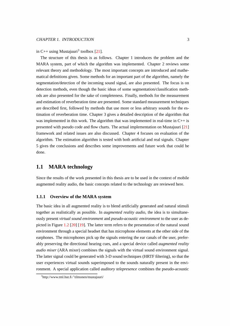
1.1 A listener in a pseudo-acoustic environment. . . . . . . . . . . . . . . . . . 4
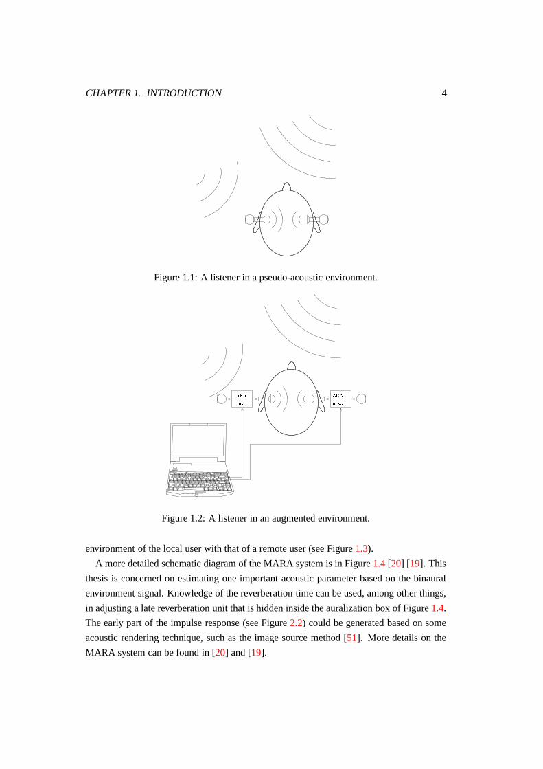
1.2 A listener in an augmented environment. . . . . . . . . . . . . . . . . . . . 4
1.3 One user experiences the sound environment heard by another user. . . . . 5
1.4 A generic diagram of an augmented reality audio system. . . . . . . . . . . 5
2.1 A linear system in time and frequency domains. . . . . . . . . . . . . . . . 9
2.2 A simplified reflectogram presentation of a room impulse response. . . . . 10
2.3 Schroeder integration curves with different upper limits. . . . . . . . . . . 15
2.4 An example of the Schroeder method applied successfully. . . . . . . . . . 15
2.5 A example of the Schroeder method applied less successfully. . . . . . . . 16
2.6 An example of fitting an optimal line to a decay curve. . . . . . . . . . . . 18
2.7 Another example of fitting an optimal line to a decay curve. . . . . . . . . . 18
2.8 A general model for signal segmentation/detection/classification/recognition. 23
2.9 Hierarchy of signal content analysis methods. . . . . . . . . . . . . . . . . 23
3.1 Flowchart of the algorithm. . . . . . . . . . . . . . . . . . . . . . . . . . . 31
3.2 The coarse segmentation algorithm in action. . . . . . . . . . . . . . . . . 35
3.3 An example of Schroeder integration with the limits Ti and Td. . . . . . . . 39
3.4 The knee point location algorithm in action. . . . . . . . . . . . . . . . . . 41
3.5 Finding the linear regression range when knee point algorithm was used. . . 44
3.6 Control window of the reverberation time estimation plugin. . . . . . . . . 46
4.1 Spectrograms of five synthetic pulses used in algorithm evaluation. . . . . . 54
xi
4.2 Short-time coherence of a synthetic convolved pulse (fc = 78
fs
2 ≈ 19.3 kHz). 55
4.3 Coherogram of a synthetic convolved pulse (fc = 78
fs
2 ≈ 19.3 kHz). . . . . 55
4.4 Short-time coherence of a synthetic convolved pulse (fc = 18
fs
2 ≈ 2.8 kHz). 56
4.5 Coherogram of a synthetic convolved pulse (fc = 18
fs
2 ≈ 2.8 kHz). . . . . . 56
4.6 Short-time coherence of a synthetic convolved pulse with averaging (fc =78
fs
2 ≈ 19.3 kHz, β = 0.8). . . . . . . . . . . . . . . . . . . . . . . . . . . 57
4.7 Coherogram of a synthetic convolved pulse with averaging (fc = 78
fs
2 ≈
19.3 kHz, β = 0.8). . . . . . . . . . . . . . . . . . . . . . . . . . . . . . . 57
4.8 Estimates of T60 for room T3 with and without least squares limit lookup
(Section 3.3.1), convolved signal. . . . . . . . . . . . . . . . . . . . . . . . 60
4.9 Three different statistics calculated from T60 estimates for room T3, con-
volved signal. . . . . . . . . . . . . . . . . . . . . . . . . . . . . . . . . . 61
4.10 Histogram of T60 estimates for room T3, convolved signal. . . . . . . . . . 61
4.11 Estimates of T60 for room A152 with and without least squares limit lookup
(Section 3.3.1), convolved signal. . . . . . . . . . . . . . . . . . . . . . . . 62
4.12 Three different statistics calculated from T60 estimates for room A152, con-
volved signal. . . . . . . . . . . . . . . . . . . . . . . . . . . . . . . . . . 62
4.13 Histogram of T60 estimates for room A152, convolved signal. . . . . . . . . 63
4.14 Estimates of T60 for room Pergola with and without least squares limit
lookup (Section 3.3.1), convolved signal. . . . . . . . . . . . . . . . . . . . 63
4.15 Three different statistics calculated from T60 estimates for room Pergola,
convolved signal. . . . . . . . . . . . . . . . . . . . . . . . . . . . . . . . 64
4.16 Histogram of T60 estimates for room Pergola, convolved signal. . . . . . . 64
4.17 Estimates of T60 for room A152 with and without least squares limit lookup
(Section 3.3.1), real recording. . . . . . . . . . . . . . . . . . . . . . . . . 66
4.18 Three different statistics calculated from T60 estimates for room A152, real
recording, line fitting range -5 to -25 dB. . . . . . . . . . . . . . . . . . . . 67
4.19 Three different statistics calculated from T60 estimates for room A152, real
recording, variable line fitting limits. . . . . . . . . . . . . . . . . . . . . . 67
4.20 Histogram of T60 estimates for room A152, real recording, line fitting range
-5 to -25 dB. . . . . . . . . . . . . . . . . . . . . . . . . . . . . . . . . . . 68
xii
4.21 Histogram of T60 estimates for room A152, real recording, variable line
fitting limits. . . . . . . . . . . . . . . . . . . . . . . . . . . . . . . . . . . 68
4.22 Three different statistics calculated from T60 estimates for room T3, real
recording, variable line fitting limits. . . . . . . . . . . . . . . . . . . . . . 69
4.23 Histogram of T60 estimates for room T3, real recording, variable line fitting
limits. . . . . . . . . . . . . . . . . . . . . . . . . . . . . . . . . . . . . . 69
A.1 Algorithm configuration for Sections 4.2 and 4.3. . . . . . . . . . . . . . . 81
A.2 Algorithm configuration for Section 4.4. . . . . . . . . . . . . . . . . . . . 82
B.1 Snaps and claps convolved with BRIR of room A152. . . . . . . . . . . . . 83
B.2 Snaps and claps convolved with BRIR of room T3. . . . . . . . . . . . . . 84
B.3 Snaps and claps convolved with BRIR of room T3 (pink noise added). . . . 84
B.4 Snaps and claps convolved with BRIR of room Pergola. . . . . . . . . . . . 85
B.5 Snaps and claps convolved with BRIR of room Pergola (pink noise added). 85
xiii
List of Tables
4.1 Reverberation times of the three acoustic spaces used in evaluation. . . . . 52
4.2 Results of T60 estimation with synthetic stimuli. . . . . . . . . . . . . . . . 54
4.3 Some statistics of T60 estimation in three different spaces using convolved
recordings. . . . . . . . . . . . . . . . . . . . . . . . . . . . . . . . . . . 60
4.4 Some statistics of T60 estimation in room A152 using a real recording. . . . 66
xiv
Chapter 1
Introduction
An ongoing trend in mobile communications is the integration of multiple physical devices
into a single portable one. The devices to be combined could be, e.g., a mobile phone,
an MP3 player, an FM radio and a digital camera. At the same time, the possibilities for
the applications are substantially increasing, also because of the increased data processing
capabilities of the devices. This calls for new application ideas and completely new usage
concepts.
One such concept is augmented reality audio (ARA), which becomes wearable aug-
mented reality audio (WARA) when the devices are worn and mobile augmented reality
audio (MARA) [20] when the devices used are portable and wireless. The basic idea of
ARA/MARA technology is to add virtual sounds to the natural sound environment experi-
enced by the user, while preserving the perception of the original environment as close to
the original as possible. The added virtual sounds should have their acoustical properties
adjusted to match those of the environment. The system and its applications are presented
in Section 1.1 of this thesis and in [20], [19] and [36].
The augmented reality audio concept also includes continuously recording the binaural
sound signal entering the ears of the user. Besides many other things, the obtained binaural
signal could be used to analyze the acoustic environment around the user. One could think
of localizing sound sources [35], recognizing the environment (e.g. home, car, restaurant)
[15] and estimating the reverberation time [49] as examples of the kind of analysis that
could be performed.
This thesis is concerned on analysis of the latter kind, namely the estimation of room
reverberation time (T60) from binaural signals. In a normal usage situation there is no a
priori knowledge about the acoustical environment or a measurement setup available. The
position of the microphones, i.e., the user, is unknown and the excitation signal can not
be controlled. The acoustical parameters of the room have to be estimated from the live
1
CHAPTER 1. INTRODUCTION 2
microphone signals containing arbitrary sounds from the environment. The goal is to de-
velop an algorithm that could give a sufficiently reliable estimate of T60 by finding suitable
sound segments from an arbitrary binaural signal and subjecting them to reverberation time
analysis. The binaural nature of the input signal should be taken into account, i.e., there
should be some inter-channel analysis steps. Different criteria for testing the suitability of
the sound segments are used. Transient sounds, such as hand claps and snaps, have favor-
able properties related to reverberation time estimation. Some of the criteria are thus related
to testing whether a certain sound event is a transient one.
The algorithm proposed in this work consists of several stages, the first of which is de-
tection of interesting sound events. The obtained signal segments are then subjected to
different analysis steps that try to decide whether the segment can be used for reverberation
time analysis and to determine the exact part of the segment that is suitable for the analysis.
The reverberation time is then calculated by using the well-known Schroeder method [52],
followed by a standard line fitting procedure to obtain the estimate. Finally, some statistical
methods are required to obtain the final estimate from an ensemble of estimates.
It is very challenging to develop an algorithm that can automatically detect the sound
events and do all necessary decisions correctly. First of all, the signals used for estimation
are completely arbitrary. Their frequency content might vary, which affects the reverber-
ation time. The reverberation time is measured from free decay, during which all sound
sources present should be silent. Therefore the areas of free decay should be somehow de-
tected from the signal. The inherently statistical nature of room reverberation also causes
some trouble, manifesting itself as variation in the reverberation time estimates. Most of
these problems are tackled in the implemented algorithm somehow.
An estimate, even a rough one, of the reverberation time of the room around the user of
an ARA system is useful for several purposes. First of all, the reverberation time can be
used as one acoustic cue for recognizing the (type of) environment the user is in. Second,
different signal processing strategies can be applied dependent on the amount of reverbera-
tion in the space that the user is in. One specific signal processing strategy is to modify the
amount of reverberation added to augmented sound events (see Chapter 1.1), according to
the estimated reverberation time of the environment, in order to make the artificially added
sound more natural. The effect of adding reverberation to spatial audio displays has been
studied previously in e.g. [54] and [13].
This work was carried out as a part of the KAMARA (Killer Applications for Mobile
Augmented Reality Audio) project that was funded by Nokia1. An offline version of the al-
gorithm was implemented in MATLAB2 and the final real-time implementation was written
1http://www.nokia.com2http://www.mathworks.com
CHAPTER 1. INTRODUCTION 3
in C++ using Mustajuuri3 toolbox [21].
The structure of this thesis is as follows. Chapter 1 introduces the problem and the
MARA system, part of which the algorithm was implemented. Chapter 2 reviews some
relevant theory and methodology. The most important concepts are introduced and mathe-
matical definitions given. Some methods for an important part of the algorithm, namely the
segmentation/detection of the incoming sound signal, are also presented. The focus is on
detection methods, even though the basic ideas of some segmentation/classification meth-
ods are also presented for the sake of completeness. Finally, methods for the measurement
and estimation of reverberation time are presented. Some standard measurement techniques
are described first, followed by methods that use more or less arbitrary sounds for the es-
timation of reverberation time. Chapter 3 gives a detailed description of the algorithm that
was implemented in this work. The algorithm that was implemented in real-time in C++ is
presented with pseudo code and flow charts. The actual implementation on Mustajuuri [21]
framework and related issues are also discussed. Chapter 4 focuses on evaluation of the
algorithm. The estimation algorithm is tested with both artificial and real signals. Chapter
5 gives the conclusions and describes some improvements and future work that could be
done.
1.1 MARA technology
Since the results of the work presented in this thesis are to be used in the context of mobile
augmented reality audio, the basic concepts related to the technology are reviewed here.
1.1.1 Overview of the MARA system
The basic idea in all augmented reality is to blend artificially generated and natural stimuli
together as realistically as possible. In augmented reality audio, the idea is to simultane-
ously present virtual sound environment and pseudo-acoustic environment to the user as de-
picted in Figure 1.2 [20] [19]. The latter term refers to the presentation of the natural sound
environment through a special headset that has microphone elements at the other side of the
earphones. The microphones pick up the signals entering the ear canals of the user, prefer-
ably preserving the directional hearing cues, and a special device called augmented reality
audio mixer (ARA mixer) combines the signals with the virtual sound environment signal.
The latter signal could be generated with 3-D sound techniques (HRTF filtering), so that the
user experiences virtual sounds superimposed to the sounds naturally present in the envi-
ronment. A special application called auditory telepresence combines the pseudo-acoustic
3http://www.tml.hut.fi/˜tilmonen/mustajuuri/
CHAPTER 1. INTRODUCTION 4
Figure 1.1: A listener in a pseudo-acoustic environment.
Figure 1.2: A listener in an augmented environment.
environment of the local user with that of a remote user (see Figure 1.3).
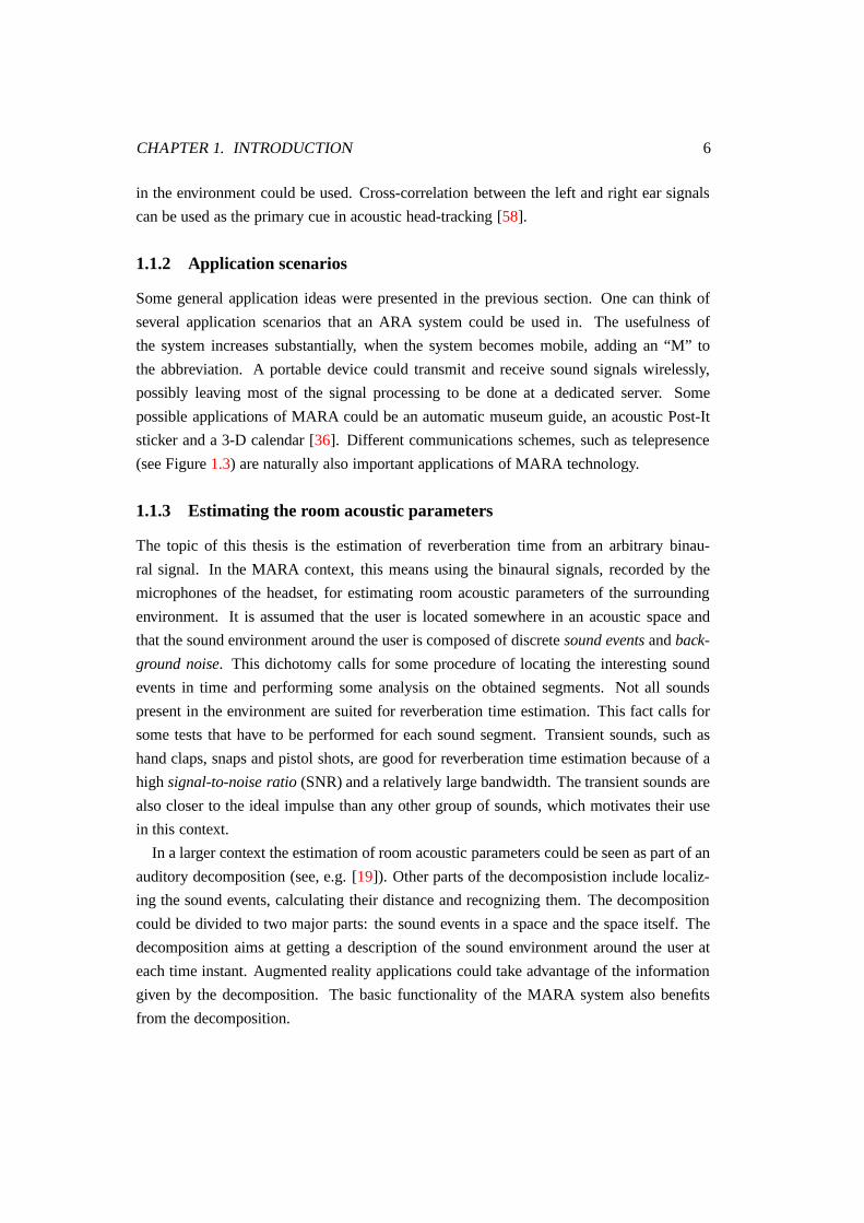
A more detailed schematic diagram of the MARA system is in Figure 1.4 [20] [19]. This
thesis is concerned on estimating one important acoustic parameter based on the binaural
environment signal. Knowledge of the reverberation time can be used, among other things,
in adjusting a late reverberation unit that is hidden inside the auralization box of Figure 1.4.
The early part of the impulse response (see Figure 2.2) could be generated based on some
acoustic rendering technique, such as the image source method [51]. More details on the
MARA system can be found in [20] and [19].
CHAPTER 1. INTRODUCTION 5
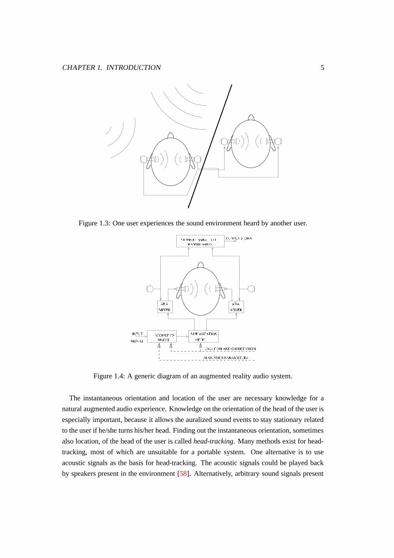
Figure 1.3: One user experiences the sound environment heard by another user.
Figure 1.4: A generic diagram of an augmented reality audio system.
The instantaneous orientation and location of the user are necessary knowledge for a
natural augmented audio experience. Knowledge on the orientation of the head of the user is
especially important, because it allows the auralized sound events to stay stationary related
to the user if he/she turns his/her head. Finding out the instantaneous orientation, sometimes
also location, of the head of the user is called head-tracking. Many methods exist for head-
tracking, most of which are unsuitable for a portable system. One alternative is to use
acoustic signals as the basis for head-tracking. The acoustic signals could be played back
by speakers present in the environment [58]. Alternatively, arbitrary sound signals present
CHAPTER 1. INTRODUCTION 6
in the environment could be used. Cross-correlation between the left and right ear signals
can be used as the primary cue in acoustic head-tracking [58].
1.1.2 Application scenarios
Some general application ideas were presented in the previous section. One can think of
several application scenarios that an ARA system could be used in. The usefulness of
the system increases substantially, when the system becomes mobile, adding an “M” to
the abbreviation. A portable device could transmit and receive sound signals wirelessly,
possibly leaving most of the signal processing to be done at a dedicated server. Some
possible applications of MARA could be an automatic museum guide, an acoustic Post-It
sticker and a 3-D calendar [36]. Different communications schemes, such as telepresence
(see Figure 1.3) are naturally also important applications of MARA technology.
1.1.3 Estimating the room acoustic parameters
The topic of this thesis is the estimation of reverberation time from an arbitrary binau-
ral signal. In the MARA context, this means using the binaural signals, recorded by the
microphones of the headset, for estimating room acoustic parameters of the surrounding
environment. It is assumed that the user is located somewhere in an acoustic space and
that the sound environment around the user is composed of discrete sound events and back-
ground noise. This dichotomy calls for some procedure of locating the interesting sound
events in time and performing some analysis on the obtained segments. Not all sounds
present in the environment are suited for reverberation time estimation. This fact calls for
some tests that have to be performed for each sound segment. Transient sounds, such as
hand claps, snaps and pistol shots, are good for reverberation time estimation because of a
high signal-to-noise ratio (SNR) and a relatively large bandwidth. The transient sounds are
also closer to the ideal impulse than any other group of sounds, which motivates their use
in this context.
In a larger context the estimation of room acoustic parameters could be seen as part of an
auditory decomposition (see, e.g. [19]). Other parts of the decomposistion include localiz-
ing the sound events, calculating their distance and recognizing them. The decomposition
could be divided to two major parts: the sound events in a space and the space itself. The
decomposition aims at getting a description of the sound environment around the user at
each time instant. Augmented reality applications could take advantage of the information
given by the decomposition. The basic functionality of the MARA system also benefits
from the decomposition.
Chapter 2
Theory and methods
This chapter reviews some of the theory behind the algorithm developed in this work. Rele-
vant basic signals and systems theory is reviewed first, followed by theoretical background
of reverberation time and the methods used in its measurement and estimation.
2.1 Signals and systems
The basis of all signal processing is the concept of signals and systems. A signal is a repre-
sentation of the evolution of a (usually physical) quantity as a function of some independent
variable, such as time or spatial location [40]. The properties of the signal change as it is
passed through a system, which can be physical, such as a room, or non-physical, such as a
digital filter implemented in a computer.
2.1.1 Categorization of signals
Signals can be categorized in many ways, most of which will not be discussed here. Real-
world signals, such as sound pressure at a certain location, exist continuously in time and
can have any amplitude value at a given instant. Such signals are usually referred to as
analog signals and will be denoted as x(t), where t represents continuous time. Digital
signals are only defined at discrete time instants and have discrete amplitude values. They
are denoted by x(n), where n is the discrete time index. This thesis is mostly concerned
with digital signals that are generated by sampling an analog sound signal at uniformly
spaced time instants. This time interval is termed sampling interval and denoted by Ts.
The inverse of the sampling interval is the sampling frequency or sample rate, denoted by
fs = 1Ts
.
Another important categorization of signals is related to their statistical properties. A
deterministic signal has each of its values fixed and the entire signal is determined by a
7
CHAPTER 2. THEORY AND METHODS 8
mathematical expression, rule or a look-up table [40]. On the contrary, a random signal can
not be predicted ahead in time with full confidence. Random signals are important in this
thesis, because most acoustical measurements result in signals of random nature.
2.1.2 Random signals
Since this thesis is mainly concerned with discrete-time signals, the treatment of random
signals will be limited to the discrete-time case. Thus a discrete-time random signal is a
sequence of numbers that is generated as the outcome of some underlying random process
[18]. The most important aspect relating to acoustical measurements is that the measured
signals are usually different realizations of a certain physical phenomenon. For a complete
description of the phenomenon, a complete set of possible realizations (an ensemble) would
be needed [28]. Usually this kind of an ensemble is not available, so time averages have
to be substituted for ensemble averages when calculating statistical measures. The former
refers to averaging a single realization over time, while the latter refers to averaging the
signal values at a fixed time over all realizations. This only applies to signals that are wide
sense stationary (WSS), meaning that the first order statistics of the signal do not change
over time. The signal is said to be ergodic if time averages can be substituted for ensemble
averages. When measuring stationary signals, it is often assumed that the phenomenon is
ergodic [28]. The signals encountered in this work can hardly be regarded as stationary,
making parameter estimation problems considerably more difficult.
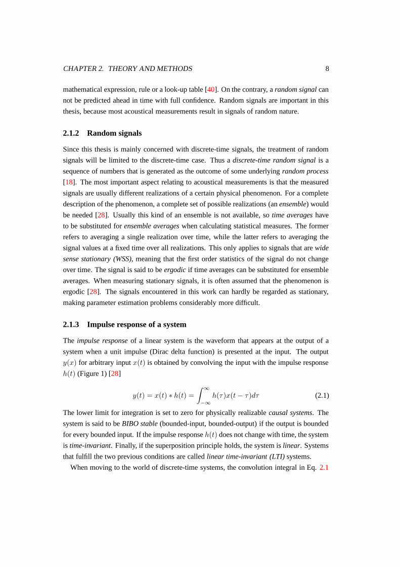
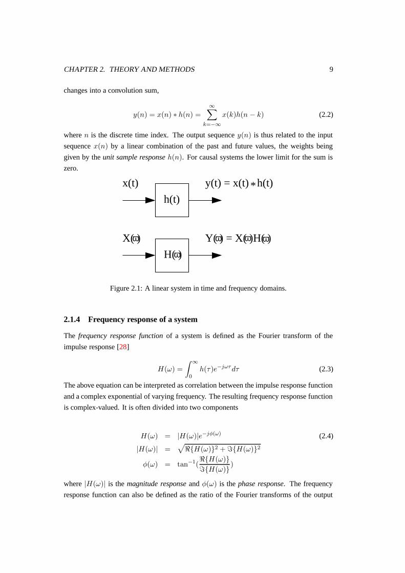
2.1.3 Impulse response of a system
The impulse response of a linear system is the waveform that appears at the output of a
system when a unit impulse (Dirac delta function) is presented at the input. The output
y(x) for arbitrary input x(t) is obtained by convolving the input with the impulse response
h(t) (Figure 1) [28]
y(t) = x(t) ∗ h(t) =
∫
∞
−∞
h(τ)x(t − τ)dτ (2.1)
The lower limit for integration is set to zero for physically realizable causal systems. The
system is said to be BIBO stable (bounded-input, bounded-output) if the output is bounded
for every bounded input. If the impulse response h(t) does not change with time, the system
is time-invariant. Finally, if the superposition principle holds, the system is linear. Systems
that fulfill the two previous conditions are called linear time-invariant (LTI) systems.
When moving to the world of discrete-time systems, the convolution integral in Eq. 2.1
CHAPTER 2. THEORY AND METHODS 9
changes into a convolution sum,
y(n) = x(n) ∗ h(n) =
∞∑
k=−∞
x(k)h(n − k) (2.2)
where n is the discrete time index. The output sequence y(n) is thus related to the input
sequence x(n) by a linear combination of the past and future values, the weights being
given by the unit sample response h(n). For causal systems the lower limit for the sum is
zero.
X( )
x(t) y(t) = x(t) h(t)*
Y( ) = X( )H( )
H( )
h(t)
ωω ω ω
ω
Figure 2.1: A linear system in time and frequency domains.
2.1.4 Frequency response of a system
The frequency response function of a system is defined as the Fourier transform of the
impulse response [28]
H(ω) =
∫
∞
0h(τ)e−jωτ dτ (2.3)
The above equation can be interpreted as correlation between the impulse response function
and a complex exponential of varying frequency. The resulting frequency response function
is complex-valued. It is often divided into two components
H(ω) = |H(ω)|e−jφ(ω) (2.4)
|H(ω)| =√
<{H(ω)}2 + ={H(ω)}2
φ(ω) = tan−1(<{H(ω)}
={H(ω)})
where |H(ω)| is the magnitude response and φ(ω) is the phase response. The frequency
response function can also be defined as the ratio of the Fourier transforms of the output
CHAPTER 2. THEORY AND METHODS 10
and input signals
H(ω) =Y (ω)
X(ω)(2.5)
2.2 Room acoustic criteria
The perception of an acoustic space can be characterized using different parameters. These
perceptual parameters are called room acoustic criteria, following the terminology used in
[45]. The core of this thesis is the estimation of the most important parameter, namely the
reverberation time.
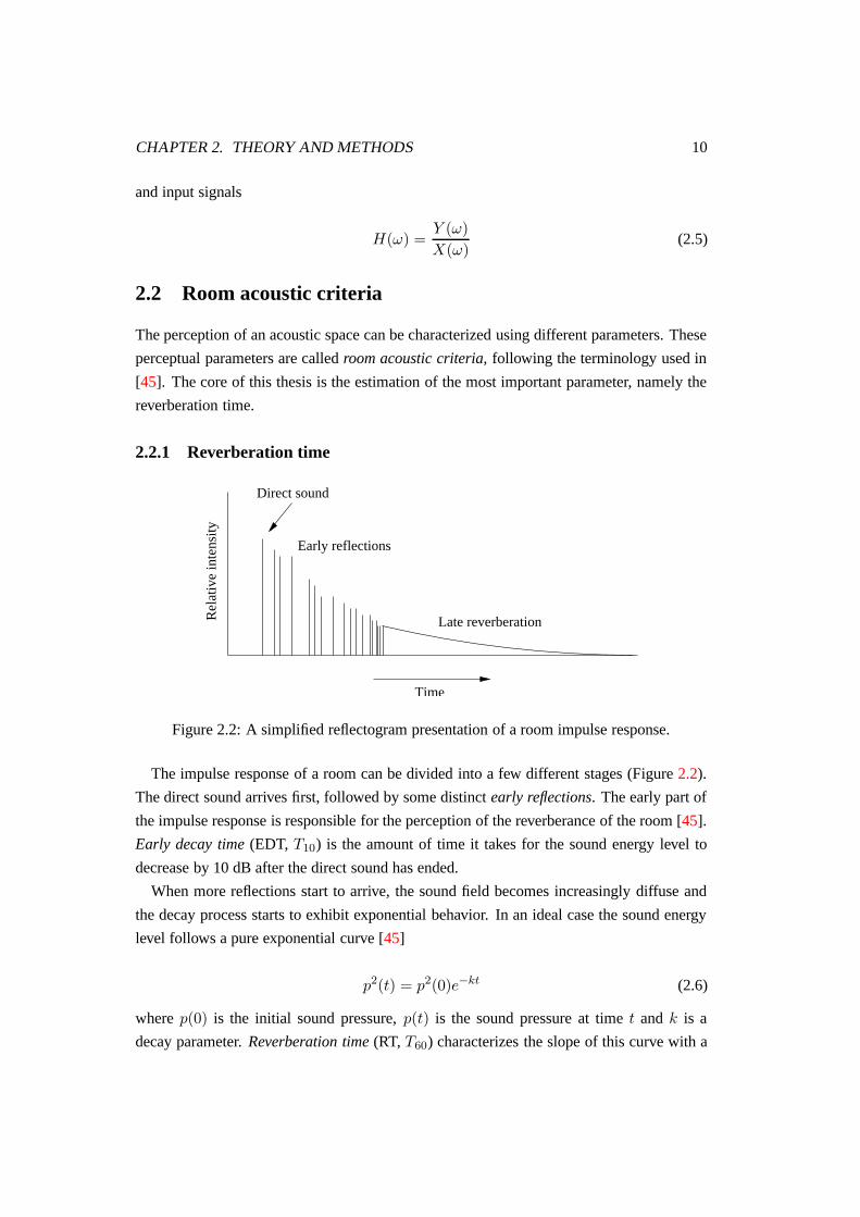
2.2.1 Reverberation time
Time
Early reflections
Rel
ativ
e in
tens
ity
Late reverberation
Direct sound
Figure 2.2: A simplified reflectogram presentation of a room impulse response.
The impulse response of a room can be divided into a few different stages (Figure 2.2).
The direct sound arrives first, followed by some distinct early reflections. The early part of
the impulse response is responsible for the perception of the reverberance of the room [45].
Early decay time (EDT, T10) is the amount of time it takes for the sound energy level to
decrease by 10 dB after the direct sound has ended.
When more reflections start to arrive, the sound field becomes increasingly diffuse and
the decay process starts to exhibit exponential behavior. In an ideal case the sound energy
level follows a pure exponential curve [45]
p2(t) = p2(0)e−kt (2.6)
where p(0) is the initial sound pressure, p(t) is the sound pressure at time t and k is a
decay parameter. Reverberation time (RT, T60) characterizes the slope of this curve with a
CHAPTER 2. THEORY AND METHODS 11
single figure and is defined as the time for the sound energy level to decay 60 dB after the
excitation has ended. If no further information is provided, T60 is assumed to be calculated
on the octave band centered at 500 Hz [50]. Usually, T60 is calculated on several different
octave bands to get some idea of the frequency behavior of the decay process of the room.
Two kinds of reverberation times are commonly used, the other one being T30, which is
the time it takes for the sound energy level to decay 30 dB after the end of the excitation.
In practice it is often not possible to measure T60 directly because the noise level is too
high for that. To enable direct comparisons between different decay measures, T10 and T30
are scaled with factors 6 and 2, respectively, to match T60. Actually, the subscripts 10,
30 and 60 simply refer to the length of the evaluation range. The different reverberation
times are always scaled to match T60. In this work no differences between different decay
times are made, because the evaluation range may vary (see Section 3.3.1). Therefore all
reverberation times, regardless of the evaluation range, will be denoted with T60 from now
on.
The simplest way of calculating the reverberation time from a measured impulse response
would be that of finding the time instant when the sound energy level falls below 60 dB
from the peak level. However, usually the noise floor is too high for this. The effect of
the direct sound and early reflections has also to be taken into account, because the early
part might decay faster than the late part of the reverberation. There might also be two or
more stages of decay with different time constants and the squared impulse response might
exhibit warbling behavior [45]. To overcome the first two problems, only the portion of the
decay curve1 between -5 dB and -35 dB (or -5 dB and -25 dB) is normally used.
Simply measuring the time interval directly from the logarithmic decay curve is usually
not accurate enough. The usual procedure is to use linear regression (described in Section
2.4) to fit a straight line to the data, possibly preceded by the Schroeder method (discussed
in Section 2.3). It should also be noted that reverberation time on different frequency bands
is often calculated and reported in addition to the average value.
The reverberation time of a room is mostly dependent on two properties of the room:
1. Volume of the room (V )
2. Absorption area of the room (A = αS, where α is the average absorption coefficient
of the room and S is the net area of the surfaces in the room)
1A few notes about the terminology should be made at this point. Decay curve may refer to either the
idealized decay curve (Eq. 2.6), its noisy real-world manifestation (squared impulse response h2(t), also
known as energy-time curve [45]) or the decay curve obtained by applying the Schroeder method presented in
Section 2.3. When there is a need to distinguish between the squared impulse response and the decay curve
obtained by the Schroeder method, the latter will be termed integration curve in this thesis. This term will be
mostly used in Chapter 3.
CHAPTER 2. THEORY AND METHODS 12
A third property that is relevant only in large rooms is air absorption. The pioneering
work by Sabine resulted in the discovery relating these properties to the decay process of
a diffuse sound field in a room. The classical formula for reverberation time (T60) will be
derived here, starting from the definition of energy density [46]
ξ =p2
r(t)
ρc2(2.7)
where pr(t) is spatially averaged sound pressure of the diffuse sound field in the room, ρ
is the density of the medium (air) and c is the sound velocity. There is a theorem stating
that the rate at which energy is produced in the room (source power) has to be equal to the
the rate at which it the energy increases throughout the room plus the rate at which it is
absorbed by the surfaces. This can be expressed as a differential equation
Π = Vdξ
dt+ ξ
c αS
4(2.8)
where Π is the power of the sound source, V dξdt is the rate at which the acoustical energy
increases in the room and ξ c αS4 is the rate at which the energy is absorbed by the surfaces
of the room. By setting Π = 0 in Eq. 2.8 and integrating, the formula for sound energy
decay is obtained as
p2r(t) = p2
r(0)e−
c αS
4Vt (2.9)
where pr(0) is the sound pressure level at time t = 0 when the sound source is shut down.
This equation, when converted to a difference in sound pressure levels, becomes
∆Lp = 10 log10
(
p2r(t)
p2r(0)
)
(2.10)
= 10 log10
(
e−c αS
4V t)
= 10
(
−c αS
4Vt
)
log10(e)
= −4.35
(
cαS
4V
)
t
(2.11)
Since at t = T60 the sound energy level should be -60 dB below the initial value, the
reverberation time is obtained as
T60 = 13.8(4V
c αS) =
55.2V
c αS≈ 0.16
V
A(2.12)
CHAPTER 2. THEORY AND METHODS 13
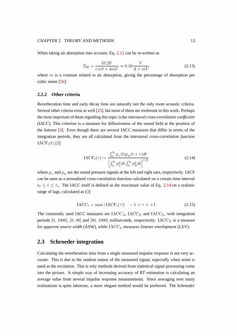
When taking air absorption into account, Eq. 2.12 can be re-written as
T60 =55.2V
c αS + 4mV≈ 0.16
V
A + mV(2.13)
where m is a constant related to air absorption, giving the percentage of absorption per
cubic meter [50].
2.2.2 Other criteria
Reverberation time and early decay time are naturally not the only room acoustic criteria.
Several other criteria exist as well [23], but most of them are irrelevant in this work. Perhaps
the most important of them regarding this topic is the interaural cross-correlation coefficient
(IACC). This criterion is a measure for diffusiveness of the sound field at the position of
the listener [3]. Even though there are several IACC measures that differ in terms of the
integration periods, they are all calculated from the interaural cross-correlation function
IACFt(t) [3]
IACFt(τ) =
∫ t2t1
pL(t)p
R(t + τ)dt
[
∫ t2t1
p2Ldt
∫ t2t1
p2Rdt
]1/2(2.14)
where pL
and pR
are the sound pressure signals at the left and right ears, respectively. IACF
can be seen as a normalized cross-correlation function calculated on a certain time interval
t0 ≤ t ≤ t1. The IACC itself is defined as the maximum value of Eq. 2.14 on a realistic
range of lags, calculated as [3]
IACCt = max | IACFt(τ)| − 1 < τ < +1 (2.15)
The commonly used IACC measures are IACCA, IACCE and IACCL, with integration
periods [0, 1000], [0, 80] and [80, 1000] milliseconds, respectively. IACCE is a measure
for apparent source width (ASW), while IACCL measures listener envelopment (LEV).
2.3 Schroeder integration
Calculating the reverberation time from a single measured impulse response is not very ac-
curate. This is due to the random nature of the measured signal, especially when noise is
used as the excitation. This is why methods derived from statistical signal processing come
into the picture. A simple way of increasing accuracy of RT estimation is calculating an
average value from several impulse response measurements. Since averaging over many
realizations is quite laborous, a more elegant method would be preferred. The Schroeder
CHAPTER 2. THEORY AND METHODS 14
method relates the ensemble average of all possible decay curves to the corresponding im-
pulse response [52]
〈y2(t)〉e =
∫
∞
t|h(τ)|2dτ =
∫
∞
0|h(τ)|2dτ −
∫ t
0|h(τ)|2dτ (2.16)
where y(t) is the decaying response (the reverberant tail), h(τ) is the impulse response of
the whole system (including the sound source, the measurement equipment and the room).
The ensemble average is indicated by 〈·〉e. Equation 2.16 makes it possible to calculate the
average decay curve from a single measured impulse response.
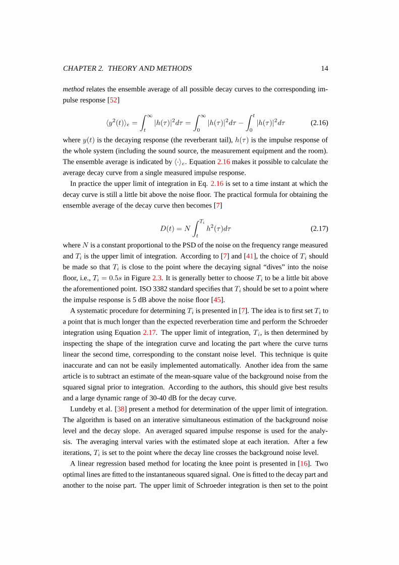
In practice the upper limit of integration in Eq. 2.16 is set to a time instant at which the
decay curve is still a little bit above the noise floor. The practical formula for obtaining the
ensemble average of the decay curve then becomes [7]
D(t) = N
∫ Ti
th2(τ)dτ (2.17)
where N is a constant proportional to the PSD of the noise on the frequency range measured
and Ti is the upper limit of integration. According to [7] and [41], the choice of Ti should
be made so that Ti is close to the point where the decaying signal “dives” into the noise
floor, i.e., Ti = 0.5s in Figure 2.3. It is generally better to choose Ti to be a little bit above
the aforementioned point. ISO 3382 standard specifies that Ti should be set to a point where
the impulse response is 5 dB above the noise floor [45].
A systematic procedure for determining Ti is presented in [7]. The idea is to first set Ti to
a point that is much longer than the expected reverberation time and perform the Schroeder
integration using Equation 2.17. The upper limit of integration, Ti, is then determined by
inspecting the shape of the integration curve and locating the part where the curve turns
linear the second time, corresponding to the constant noise level. This technique is quite
inaccurate and can not be easily implemented automatically. Another idea from the same
article is to subtract an estimate of the mean-square value of the background noise from the
squared signal prior to integration. According to the authors, this should give best results
and a large dynamic range of 30-40 dB for the decay curve.
Lundeby et al. [38] present a method for determination of the upper limit of integration.
The algorithm is based on an interative simultaneous estimation of the background noise
level and the decay slope. An averaged squared impulse response is used for the analy-
sis. The averaging interval varies with the estimated slope at each iteration. After a few
iterations, Ti is set to the point where the decay line crosses the background noise level.
A linear regression based method for locating the knee point is presented in [16]. Two
optimal lines are fitted to the instantaneous squared signal. One is fitted to the decay part and
another to the noise part. The upper limit of Schroeder integration is then set to the point
CHAPTER 2. THEORY AND METHODS 15
where the two lines intersect. This method is not applicable for automatic reverberation
time estimation since it involves the user manually choosing one of the limits of line fitting.
0 0.1 0.2 0.3 0.4 0.5 0.6 0.7 0.8 0.9−80
−70
−60
−50
−40
−30
−20
−10
0
10
Time / s
Ene
rgy
/ dB
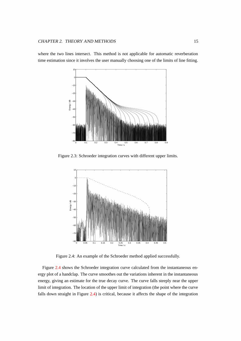
Figure 2.3: Schroeder integration curves with different upper limits.
0 0.05 0.1 0.15 0.2 0.25 0.3 0.35 0.4 0.45 0.5−80
−70
−60
−50
−40
−30
−20
−10
0
10
Ene
rgy
/ dB
Time / s
Figure 2.4: An example of the Schroeder method applied successfully.
Figure 2.4 shows the Schroeder integration curve calculated from the instantaneous en-
ergy plot of a handclap. The curve smoothes out the variations inherent in the instantaneous
energy, giving an estimate for the true decay curve. The curve falls steeply near the upper
limit of integration. The location of the upper limit of integration (the point where the curve
falls down straight in Figure 2.4) is critical, because it affects the shape of the integration
CHAPTER 2. THEORY AND METHODS 16
0 0.1 0.2 0.3 0.4 0.5 0.6 0.7 0.8 0.9−80
−70
−60
−50
−40
−30
−20
−10
0
10
Ene
rgy
/ dB
Time / s
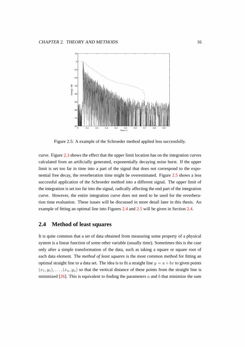
Figure 2.5: A example of the Schroeder method applied less successfully.
curve. Figure 2.3 shows the effect that the upper limit location has on the integration curves
calculated from an artificially generated, exponentially decaying noise burst. If the upper
limit is set too far in time into a part of the signal that does not correspond to the expo-
nential free decay, the reverberation time might be overestimated. Figure 2.5 shows a less
successful application of the Schroeder method into a different signal. The upper limit of
the integration is set too far into the signal, radically affecting the end part of the integration
curve. However, the entire integration curve does not need to be used for the reverbera-
tion time evaluation. These issues will be discussed in more detail later in this thesis. An
example of fitting an optimal line into Figures 2.4 and 2.5 will be given in Section 2.4.
2.4 Method of least squares
It is quite common that a set of data obtained from measuring some property of a physical
system is a linear function of some other variable (usually time). Sometimes this is the case
only after a simple transformation of the data, such as taking a square or square root of
each data element. The method of least squares is the most common method for fitting an
optimal straight line to a data set. The idea is to fit a straight line y = a+ bx to given points
(x1, y1), . . . , (xn, yn) so that the vertical distance of these points from the straight line is
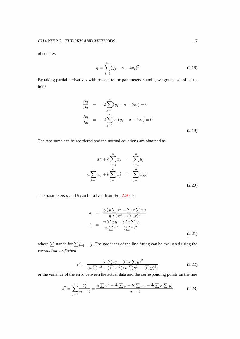
minimized [26]. This is equivalent to finding the parameters a and b that minimize the sum
CHAPTER 2. THEORY AND METHODS 17
of squares
q =
n∑
j=1
(yj − a − bxj)2 (2.18)
By taking partial derivatives with respect to the parameters a and b, we get the set of equa-
tions
∂q
∂a= −2
n∑
j=1
(yj − a − bxj) = 0
∂q
∂b= −2
n∑
j=1
xj(yj − a − bxj) = 0
(2.19)
The two sums can be reordered and the normal equations are obtained as
an + b
n∑
j=1
xj =
n∑
j=1
yj
an
∑
j=1
xj + bn
∑
j=1
x2j =
n∑
j=1
xjyj
(2.20)
The parameters a and b can be solved from Eq. 2.20 as
a =
∑
y∑
x2 −∑
x∑
xy
n∑
x2 − (∑
x)2
b =n
∑
xy −∑
x∑
y
n∑
x2 − (∑
x)2
(2.21)
where∑
stands for∑n
j=1 . . .j . The goodness of the line fitting can be evaluated using the
correlation coefficient
r2 =(n
∑
xy −∑
x∑
y)2
(n∑
x2 − (∑
x)2) (n∑
y2 − (∑
y)2)(2.22)
or the variance of the error between the actual data and the corresponding points on the line
s2 =
n∑
j=1
e2j
n − 2=
n∑
y2 − 1n
∑
y − b(∑
xy − 1n
∑
x∑
y)
n − 2(2.23)
CHAPTER 2. THEORY AND METHODS 18
0 0.05 0.1 0.15 0.2 0.25 0.3 0.35 0.4 0.45 0.5−80
−70
−60
−50
−40
−30
−20
−10
0
10
Ene
rgy
/ dB
Time / s
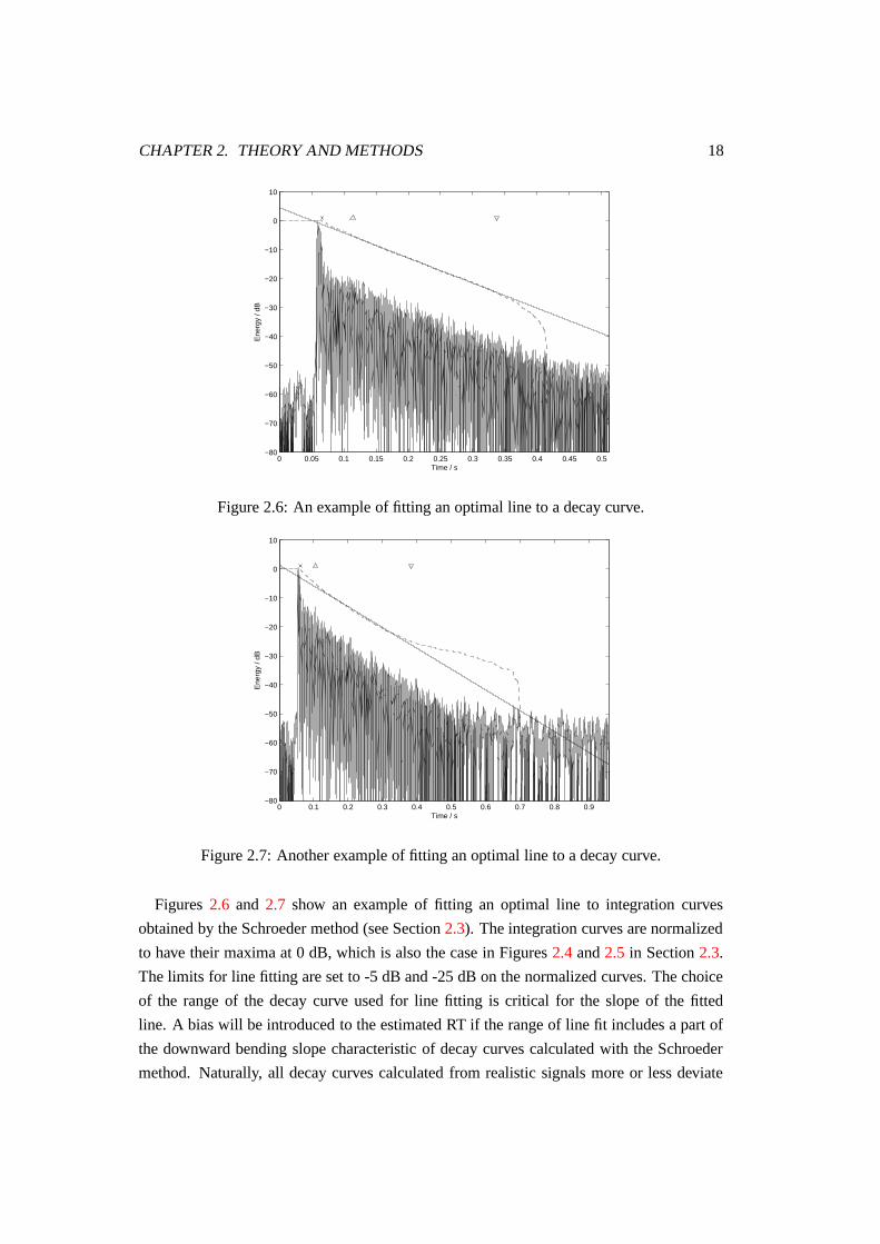
Figure 2.6: An example of fitting an optimal line to a decay curve.
0 0.1 0.2 0.3 0.4 0.5 0.6 0.7 0.8 0.9−80
−70
−60
−50
−40
−30
−20
−10
0
10
Ene
rgy
/ dB
Time / s
Figure 2.7: Another example of fitting an optimal line to a decay curve.
Figures 2.6 and 2.7 show an example of fitting an optimal line to integration curves
obtained by the Schroeder method (see Section 2.3). The integration curves are normalized
to have their maxima at 0 dB, which is also the case in Figures 2.4 and 2.5 in Section 2.3.
The limits for line fitting are set to -5 dB and -25 dB on the normalized curves. The choice
of the range of the decay curve used for line fitting is critical for the slope of the fitted
line. A bias will be introduced to the estimated RT if the range of line fit includes a part of
the downward bending slope characteristic of decay curves calculated with the Schroeder
method. Naturally, all decay curves calculated from realistic signals more or less deviate
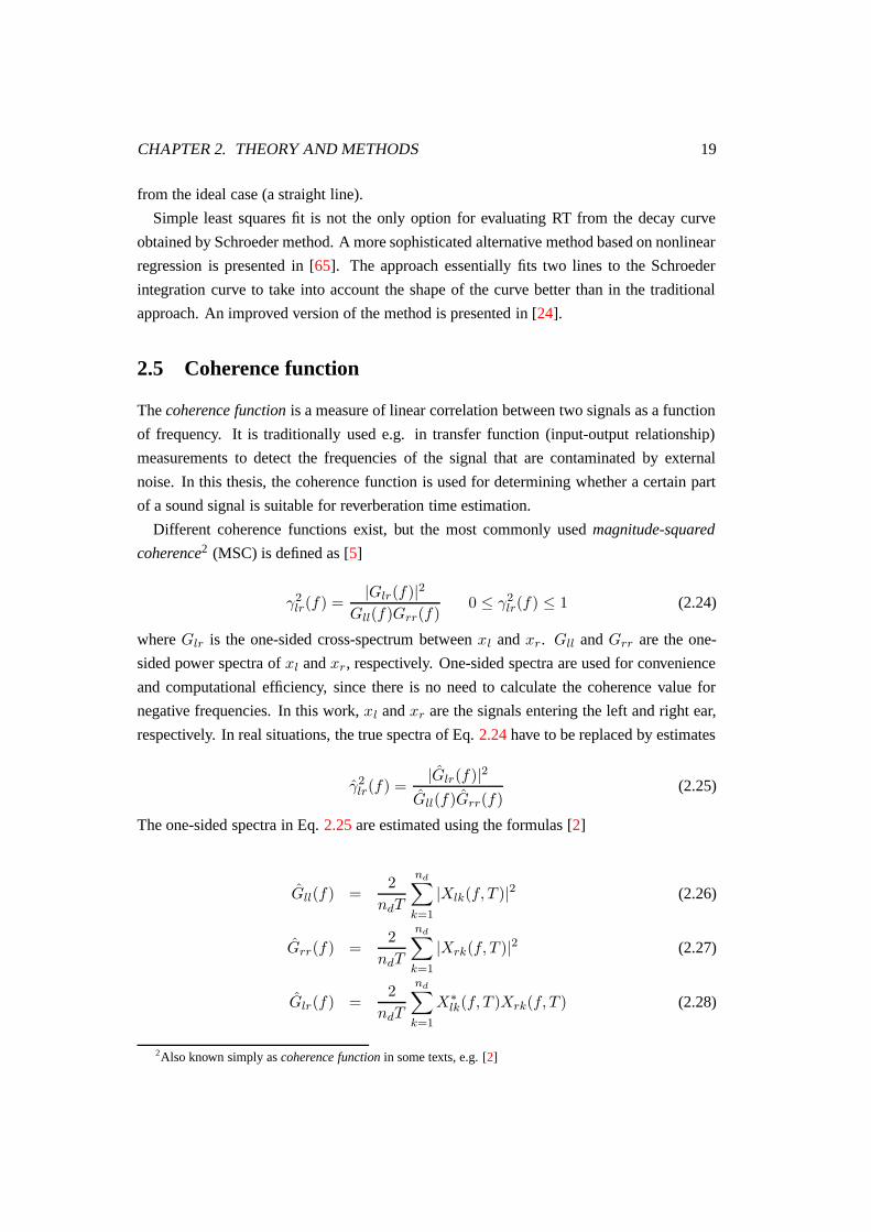
CHAPTER 2. THEORY AND METHODS 19
from the ideal case (a straight line).
Simple least squares fit is not the only option for evaluating RT from the decay curve
obtained by Schroeder method. A more sophisticated alternative method based on nonlinear
regression is presented in [65]. The approach essentially fits two lines to the Schroeder
integration curve to take into account the shape of the curve better than in the traditional
approach. An improved version of the method is presented in [24].
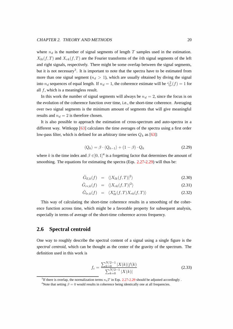
2.5 Coherence function
The coherence function is a measure of linear correlation between two signals as a function
of frequency. It is traditionally used e.g. in transfer function (input-output relationship)
measurements to detect the frequencies of the signal that are contaminated by external
noise. In this thesis, the coherence function is used for determining whether a certain part
of a sound signal is suitable for reverberation time estimation.
Different coherence functions exist, but the most commonly used magnitude-squared
coherence2 (MSC) is defined as [5]
γ2lr(f) =
|Glr(f)|2
Gll(f)Grr(f)0 ≤ γ2
lr(f) ≤ 1 (2.24)
where Glr is the one-sided cross-spectrum between xl and xr. Gll and Grr are the one-
sided power spectra of xl and xr, respectively. One-sided spectra are used for convenience
and computational efficiency, since there is no need to calculate the coherence value for
negative frequencies. In this work, xl and xr are the signals entering the left and right ear,
respectively. In real situations, the true spectra of Eq. 2.24 have to be replaced by estimates
γ2lr(f) =
|Glr(f)|2
Gll(f)Grr(f)(2.25)
The one-sided spectra in Eq. 2.25 are estimated using the formulas [2]
Gll(f) =2
ndT
nd∑
k=1
|Xlk(f, T )|2 (2.26)
Grr(f) =2
ndT
nd∑
k=1
|Xrk(f, T )|2 (2.27)
Glr(f) =2
ndT
nd∑
k=1
X∗
lk(f, T )Xrk(f, T ) (2.28)
2Also known simply as coherence function in some texts, e.g. [2]
CHAPTER 2. THEORY AND METHODS 20
where nd is the number of signal segments of length T samples used in the estimation.
Xlk(f, T ) and Xrk(f, T ) are the Fourier transforms of the kth signal segments of the left
and right signals, respectively. There might be some overlap between the signal segments,
but it is not necessary3 . It is important to note that the spectra have to be estimated from
more than one signal segment (nd > 1), which are usually obtained by diving the signal
into nd sequences of equal length. If nd = 1, the coherence estimate will be γ2lr(f) = 1 for
all f , which is a meaningless result.
In this work the number of signal segments will always be nd = 2, since the focus is on
the evolution of the coherence function over time, i.e., the short-time coherence. Averaging
over two signal segments is the minimum amount of segments that will give meaningful
results and nd = 2 is therefore chosen.
It is also possible to approach the estimation of cross-spectrum and auto-spectra in a
different way. Wittkopp [63] calculates the time averages of the spectra using a first order
low-pass filter, which is defined for an arbitrary time series Qk as [63]:
〈Qk〉 = β · 〈Qk−1〉 + (1 − β) · Qk (2.29)
where k is the time index and β ∈]0, 1]4 is a forgetting factor that determines the amount of
smoothing. The equations for estimating the spectra (Eqs. 2.27-2.29) will thus be:
Gll,k(f) = 〈|Xlk(f, T )|2〉 (2.30)
Grr,k(f) = 〈|Xrk(f, T )|2〉 (2.31)
Glr,k(f) = 〈X∗
lk(f, T )Xrk(f, T )〉 (2.32)
This way of calculating the short-time coherence results in a smoothing of the coher-
ence function across time, which might be a favorable property for subsequent analysis,
especially in terms of average of the short-time coherence across frequency.
2.6 Spectral centroid
One way to roughly describe the spectral content of a signal using a single figure is the
spectral centroid, which can be thought as the center of the gravity of the spectrum. The
definition used in this work is
fc =
∑N/2−1k=0 |X(k)|f(k)∑N/2−1
k=0 |X(k)|(2.33)
3If there is overlap, the normalization terms ndT in Eqs. 2.27-2.29 should be adjusted accordingly .4Note that setting β = 0 would results in coherence being identically one at all frequencies.
CHAPTER 2. THEORY AND METHODS 21
where N is the length of the DFT, X(k) is the DFT of the signal to be analyzed and f(k)
is the frequency (in Hz) corresponding to the discrete frequency bin k.
The spectral centroid is usually attributed to the perceived brightness of the sound. A
high value of the centroid indicates that there is considerable high frequency content in the
signal, which is usually perceived as brightness in the sound.
2.7 Signal detection, segmentation and classification
Before the estimation of reverberation time can take place, it has to be decided which parts
of the signal will be used for the estimation. That is, the relevant sound events have to be
detected from the sound signals and the suitability of the obtained segments for reverbera-
tion time estimation has to be assessed (this will be considered in Section 3.2). Methods for
signal detection, segmentation and classification will be presented in this section.
Audio signal segmentation and detection methods fall into two categories: general seg-
mentation/detection methods and segmentation/detection methods for a specific class of
sounds (e.g. speech). Methods from both categories will be presented in this chapter, even
though the focus will be on methods with general applicability. Another way of categorizing
the methods would be by features that are used in segmentation/detection. Some methods
rely on a single feature, the most obvious one being the short-time energy of the signal.
More advanced methods use either multi-dimensional features (such as time-frequency rep-
resentations (TFRs), e.g. short-time Fourier transforms) or a combination of several dif-
ferent features calculated from short-time signal windows. The same set of features could
also be used for signal classification. A general model that applies to signal segmentation,
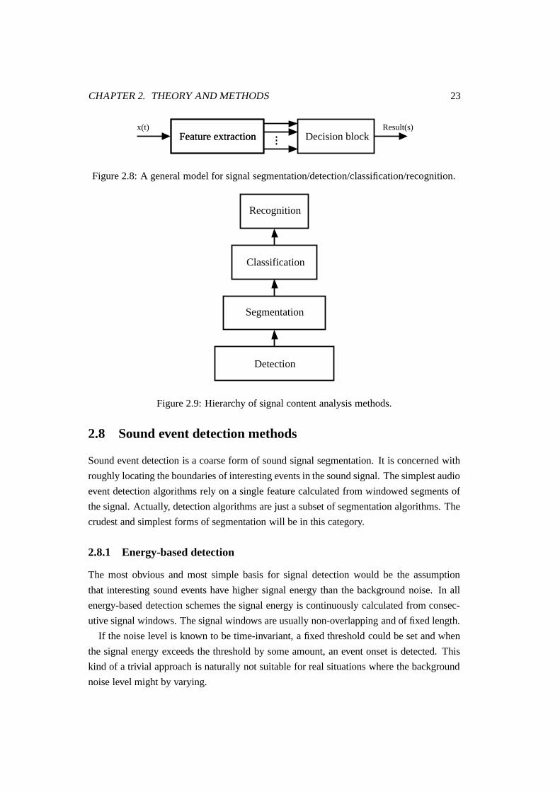
classification and detection alike, is presented in Figure 2.8.
The detection of speech, voice activity detection (VAD), is a very important and much
researched sub-topic of general audio signal segmentation and detection. The importance of
VAD is due to speech being the signal of interest that is to be transmitted in communications
applications, most importantly cellular phone networks. The channel capacity has to be
used as effectively as possible and thus transmitting useless information, i.e., noise, has to
be avoided. This can be accomplished by detecting the time regions with voice activity
in the signal picked up by the microphone. The VAD methods mostly fall outside of the
scope of this work, because of their limited applicability to detecting sound events other
than speech.
A few notes on the terminology should be made at this point. Audio signal segmentation
usually refers to the process of identifying changes in signal content and is often followed
by recognition or classification of the segments into discrete classes. The term is often used
in the area of multimedia indexing and speech processing. Signal segmentation in general
CHAPTER 2. THEORY AND METHODS 22
refers to locating the boundaries of change of a piecewise stationary signal, thus segment-
ing it into homogenous regions. Sound event detection5 refers to locating interesting sound
events that are then subjected to further processing, which could be classification or some
other form of analysis. One important part of the work described in this thesis was to find
a suitable way to detect important sound events from the continuous environmental sound
signal and subject them to analysis of room reverberation time. Thus the word detection
is more appropriate in this context, since segmentation is only concerned with finding any
significant changes in signals, usually in statistical sense. However, the terms detection and
segmentation will be used synonymously in this thesis, even though sound event detection
can also be seen as a front-end to segmentation and classification, which is exactly the ap-
proach taken in this work. The idea is to first roughly pick the possibly interesting sound
events and then do further processing, i.e., classification and segmentation on them. Sec-
tions 3.1.1 and 3.1.2 describe the sound event detection and segmentation algorithms used
in this work. It should be noted that the former will be termed coarse segmentation and the
latter fine segmentation starting from Chapter 3.
It is important to realize that all methods, whether termed detection, segmentation, clas-
sification or recognition, all have the basic structure presented in Figure 2.8. Different
short-time features are calculated from an input signal, followed by a decision block that
gives the result of the analysis as a function of time. One hierarchy of the four classes of
methods can be found in Figure 2.9. Detection is the crudest form of signal content anal-
ysis, being only concerned with roughly locating possibly interesting events in the signal.
Segmentation is more detailed analysis aiming at dividing the signal into homogenous re-
gions, with respect to some feature(s), e.g. the short-time frequency content. Classification
puts each segment, or a combination of segments, into discrete categories. Example cate-
gories could be “speech”, “music”, “environmental sounds” and “silence”. Recognition is a
more accurate form of classification attempting to recognize the sound more or less exactly.
For example, the category of environmental sounds might include “dog bark”, “car wheel
noise”, “crickets”, “bird song” and “unknown environmental sound”. Even though the rela-
tionships between the different hierarchy levels in Figure 2.9 are unidirectional, there could
be interaction from a higher to a lower level as well.
The area of signal segmentation and detection is so broad that only a small part of the
available methods will be reviewed here. The emphasis will be on methods that are relevant
in this work.5The term “detection” usually refers to detecting a known signal buried in noise in the area of telecommu-
nications signal processing.
CHAPTER 2. THEORY AND METHODS 23
Decision blockFeature extractionx(t)
Feature extractionResult(s)
Figure 2.8: A general model for signal segmentation/detection/classification/recognition.
Recognition
Classification
Segmentation
Detection
Figure 2.9: Hierarchy of signal content analysis methods.
2.8 Sound event detection methods
Sound event detection is a coarse form of sound signal segmentation. It is concerned with
roughly locating the boundaries of interesting events in the sound signal. The simplest audio
event detection algorithms rely on a single feature calculated from windowed segments of
the signal. Actually, detection algorithms are just a subset of segmentation algorithms. The
crudest and simplest forms of segmentation will be in this category.
2.8.1 Energy-based detection
The most obvious and most simple basis for signal detection would be the assumption
that interesting sound events have higher signal energy than the background noise. In all
energy-based detection schemes the signal energy is continuously calculated from consec-
utive signal windows. The signal windows are usually non-overlapping and of fixed length.
If the noise level is known to be time-invariant, a fixed threshold could be set and when
the signal energy exceeds the threshold by some amount, an event onset is detected. This
kind of a trivial approach is naturally not suitable for real situations where the background
noise level might by varying.
CHAPTER 2. THEORY AND METHODS 24
The varying background noise level should be taken into account somehow when detect-
ing audio events based on the signal energy level only. The most straightforward idea is to
calculate the signal energy on a fixed-length signal window. The mean short-term signal
energy computed in the previous signal frames is used as the reference. If the signal energy
in the current frame exceeds the reference by a certain amount, a new event is detected.
The mean of the signal energy can also be replaced by the median over the previous signal
frames.
For more reliable detection of events, the time variations of the noise level can be taken
into account [60]. The energy prediction method uses calculated energy values from a
number of previous windows to predict the energy value for the current window. If the
estimate differs from the true value by certain amount, an event is detected. The prediction
is done using the spline interpolation method [26] to extrapolate the next energy value
from the past measurements. The details on how exactly this is done are not given in [60].
Naturally, any other interpolation (or prediction) method could be used besides splines. The
abovementioned detection method based on the average of short-time energy could also be
thought as a predictive interpolation method (or more precisely, extrapolation method), even
if a simple one. In that case the next short-time energy value is predicted to stay close to
the average across a few frames.
2.8.2 Cross-correlation based detection
The similarity between two signals can be measured by evaluating the cross-correlation
function between the signals. By thresholding the maximum value of the cross-correlation
function calculated between two consecutive signal windows, abrupt changes in the signal
statistics can be detected as minima in the sequence of maximum cross-correlation values
[60] [59]. If the energies of the signal windows are normalized to have a maximum value of
one before calculating the correlations, the method will be suitable for detecting transients,
because the short onset will cause the rest of the energy values of the window to be scaled
down to very small values. This will cause the sequences of correlation maxima to have a
steep local minimum at the transient location.
This method can also be seen from the perspective of prediction. It is predicted that the
correlation properties of the signal stay the same until something interesting, i.e., an event,
happens. Yet another point of view would be that of signals and systems (see Section 2.1).
The reverberation time is a property of the system and thus it can not be estimated when the
output signal of the system is stationary. When there is a change in the output, a property
of the system (RT in this case) can be estimated if some conditions (such as a high enough
SNR) are met.
CHAPTER 2. THEORY AND METHODS 25
2.9 Signal classification and segmentation methods
When the interest in the signal content is not confined to its overall energy or some other
simple measure, more advanced methods are needed. This section reviews some common
methods that are used for signal segmentation and classification. These two tasks are of-
ten interconnected by the fact that the same or partially same set of features is used by
both. Segmentation can also appear as a “byproduct” of classification, because the segment
boundaries are at the time instants at which the classification result changes. The cate-
gorization presented here is not very strict, many methods might actually fall into several
categories.
Since recognition is just a more accurate form of classification, it will not be treated sep-
arately in this thesis. Many of the methods presented here can also be used in recognition,
even though recognition usually requires more features than classification to discriminate
between the larger number of categories. Speech recognition is not treated here at all, even
though some of the methods presented here are used in that area as well.
2.9.1 Pattern recognition based approaches
Since audio segmentation and classification can be seen as a pattern recognition problem,
methods from that field have been applied to the problem by many authors, including [64]
[34], [6], [33] and [44]. The usual procedure common to all approaches of this kind is to
calculate some features from short-time signal windows and then pass the obtained feature
vector to a classifier. The segmentation then follows from changes in the classification
result. The actual classification of the segments into discrete categories might follow as
the next separate stage. It is also common that a thin line exists between segmentation
and classification. For example, the classification module might first discriminate between
speech and non-speech signal (which is actually voice activity detection, see Section 2.9.5),
followed by classification of the non-speech category into environmental sounds, music
and silence [37]. The actual segmentation then follows from combining the results of the
classified shorter segments.
2.9.2 Hidden Markov model based approaches
The time evolution of the statistics of a signal can be taken into account as an additional
“feature” to increase recognition performance. A popular way to do this is to use hidden
Markov models (HMMs) [47] as classifiers. The basic idea is that the statistics of the signal
are modeled as states, to which initial state probabilities and state transition probabilities are
assigned. The word “hidden” comes from the fact that the current state is not observable.
Instead, an output is observed with a certain probability. The output can be e.g. a feature
CHAPTER 2. THEORY AND METHODS 26
vector calculated from the signal. When using hidden Markov models as classifiers, the
model has to be trained first, a procedure to which several algorithms have been developed.
One model is trained for each class. A given observation sequence is assigned to the class
for which the model score (likelihood) calculated from the sequence is greatest. Some
examples of using HMMs for audio signal classification can be found in e.g. [15] [14] [44].
2.9.3 Machine learning based segmentation
One subset of pattern recognition based approaches are machine learning based methods
[11] [12]. In practice this means applying support vector machines (SVM) to the segmen-
tation process. The idea is to continuously teach a support vector machine classifier with
features calculated from a number of previous signal windows and test the current signal
frame features on the SVM classifier. If the SVM decides that the current signal segment
does not belong to the class defined by the data set used for teaching, a signal segment
boundary is detected. The features are usually based on time-frequency representations of
the signals, e.g. spectrograms or other time-frequency distributions.
Other machine learning methods, such as multi-layer perceptrons (MLPs), could possibly
be used instead of SVMs, even though not reported in literature.
2.9.4 Time-frequency representation based abrupt change detection
There exists several papers on non-parametric statistical abrupt change detection based on
different measures calculated from time-frequency representations of the signals [29] [30]
[31] [55]. The idea is to calculate a stationarity index at a certain time instant. The station-
arity index compares slices of two time-frequency representations around the current time
instant using some distance measure. A high value indicates that there is a sudden change
in the spectral content of the signal at the current time instant. Yet again, this could be seen
as one form of prediction.
2.9.5 Voice activity detection (VAD)
Voice activity detection (VAD) is a category for methods for deciding whether or not there
is speech present in a given signal frame. A multitude of methods are mentioned in the
literature [56]. However, the common idea in most methods is to choose features that are
found to discriminate well between speech and non-speech waveforms and use them in
a classifier. Most most VAD methods are thus based on pattern recognition (see Section
2.9.1).
CHAPTER 2. THEORY AND METHODS 27
2.10 Reverberation time estimation methods
The main task of this work is to estimate the room reverberation time (T60) using arbitrary
binaural signals. This section reviews some methods related to reverberation time estima-
tion, starting from standard measurement techniques, in which the excitation signal can
be controlled. Some methods that use more or less arbitrary environment signals as the
excitation are described next.
2.11 Estimation methods with controlled excitation
All standard room acoustic measurements methods involve the possibility to send a con-
trolled excitation signal to the acoustic space and the possibility to measure the response
signal. The impulse response is then derived mathematically based on the excitation signal
and the measured signals. Sometimes the excitation signal is not completely in control, but
can be measured simultaneously with the response signal (two-channel measurement). The
reverberation time is obtained from the measured room impulse response (RIR) by meth-
ods such as the method of least squares and/or Schroeder method (see Sections 2.3 and
2.4). The most common types of excitation signals are an impulse (pistol shot), a swept
sine wave [42] and the maximum length sequence (MLS) [53]. A presentation of some
typical excitation signals can be found in [45].
2.11.1 MLS
The MLS method uses a pseudo-random deterministic binary sequence as the excitation
signal. The sequence has special properties that allow an efficient calculation of the impulse
response by calculating a circular cross-correlation between the excitation and the response
signals. The fast Hadamard transform (FHT) can be used for efficient calculation of the
cross-correlation. The MLS method has some properties that make it attractive for impulse
response measurements, such as a high signal-to-noise ratio, the possibility to calculate very
long impulse responses and computational efficiency. However, much of the former hype
around MLS has vanished with the increase of computational power and memory capacity
of computers [42].
2.11.2 Sweep
The sweep method uses swept sine waves as the excitation signals. As with all excitation
signals used in measurements, the excitation should include all frequencies of interest. The
swept sine waves typically move from low to high frequencies, either in linear or logarith-
mic fashion. The advantages of the sweep method over MLS are higher immunity against
CHAPTER 2. THEORY AND METHODS 28
time variance and distortion. The immunity against harmonic distortion makes it possible
to attain a significantly higher signal-to-noise ratio than with the MLS method, without
introducing distortion artifacts to the impulse response [42]. Thus the sweep method is es-
pecially suitable for measuring (binaural) impulse responses for high-quality auralization
purposes, where an SNR higher than 90 dB is required [42]. Non-idealities in the measure-
ment chain can also be easily compensated in the sweep measurements.
2.12 Estimation methods without controlled excitation
Often it is desirable to get an idea of what the reverberation time of a concert hall is at the
situation where it is used, i.e., with audience and musicians playing. Measurement methods
based on controlled excitation signals (Section 2.11) cannot be used in most cases. MLS
could be used because the excitation signal could be played back at an inaudible level.
However, very long measurement periods would be required [17]. With applications such
as hearing aids it would be totally unfeasible to actively generate an artificial test signal into
the environment. Methods that use sounds that are already present in the environment, e.g.
speech and music, for estimation of the reverberation time are therefore needed. Not very
many such methods have been proposed in the literature and it seems that this area of room
acoustical analysis is constantly evolving.
Using passively received sounds as the basis for room acoustics analysis causes extra
difficulties that are not present when using an impulse response measured with dedicated
equipment. It is unrealistic to set a goal of estimating the room acoustic parameters to the
same precision. With the focus on reverberation time, in applications such as intelligent
hearing aids it is enough to know only roughly how reverberant the current environment is
[48].
The methods presented in this section are divided into two categories according to a
taxonomy presented in [49]. Partially blind methods do require some a priori knowledge
about the room or the signal or some form of segmentation procedure to find the interesting
sounds in the environment. The algorithm developed in this work (see Chapter 3) belongs
to this category. Blind methods require minimal amount (if none) of a priori knowledge.
The maximum likelihood (ML) estimation based method in [49] belongs to this category,
as well as all blind deconvolution techniques, which give the room impulse response as a
byproduct.
2.12.1 Partially blind methods
A method of using musical signals for the estimation of reverberation was presented in [17].
The method is based on the autocorrelation function of the reverberated musical signal. The
CHAPTER 2. THEORY AND METHODS 29
idea is that the envelope of the autocorrelation function can not decay faster than the room
impulse response. Thus the reverberation time can be calculated from the envelope of
the autocorrelation function of the reverberated signal. Averaging over many estimates is
naturally needed and unsuitable signal sections have to be discarded in advance.
An interesting approach for RT estimation is to use artificial neural networks for the
estimation procedure [10]. The idea is to train a multilayer feedforward network with a
large number of artificially created test signals that have known reverberation times. The
test signals used in [10] are short speech utterances convolved with artificially generated
room impulse responses of varying reverberation times. Short time RMS values are used
as the features. The trained network should be able to estimate the reverberation time
when the same speech utterances are spoken in an acoustic space. The method does not
currently work with unrestricted speech or arbitrary signal, which limits the applicability of
the method.
A dereverberation method that includes estimation of the reverberation time is presented
in [32]. The algorithm presented consists of locating the parts of the signal with exponen-
tial decay and the estimating reverberation time from the obtained segments. A smoothed
energy envelope is used for the calculations. The details of the detection of decaying signal
parts are not given in [32].
Baskind and Warusfel mention a method for reverberation time estimation in [1]. The
method is based on the idea of locating the areas of decay from an RMS plot of the sig-
nal and then calculating the Schroeder integral from each segment. The RT estimates are
derived from the decay curves by linear regression. The final RT estimate is derived by
discarding values that are too far from the mean and then choosing the minimum from the
remaining values. It is notable that this method is the only one (of the methods presented
here) which uses binaural signals for the analysis. However, the binaural nature is exploited
only so that two estimates are calculated for each segment and the mean of the estimations is
taken. The use of the interaural correlation function is also postulated in [1] to discriminate
between free decay and the resonance of a sound source.
A quite similar automatic reverberation time estimation method based on Schroeder in-
tegration was presented in [61]. The idea is to calculate the decay curve by the Schroeder
method using overlapping windows. The decay curve is calculated only when the energy of
the current window is smaller than that of the previous window, indicating that the sound
energy is decaying. This reduces the number of false estimates. An optimal line is fitted to
each decay curve using the least squares method and the final RT estimate is derived as the
maximum of a histogram of estimates. The method is quite simple and seems to depend on
the window length, because a too long or short window will cause bias in the decay curves
and the fitted lines.
CHAPTER 2. THEORY AND METHODS 30
2.12.2 Blind methods
All blind deconvolution methods, whether or not related to room acoustics, give the impulse
response of the system as a byproduct. By deconvolving the impulse response out of a sig-
nal recorded in an acoustic space, reverberation time can be calculated from the response by
standard methods such as the Schroeder method. Different approaches for blind deconvo-
lution exist, some being related to blind dereverberation. Blind deconvolution only works
when the impulse response is minimum-phase, a condition that is not fulfilled in most real
rooms [49]. This limits the applicability of the method.
A novel approach for a completely blind maximum likelihood (ML) estimation of room
reverberation time was proposed in [49]. A computationally efficient version of the algo-
rithm has also been developed by the same authors [48]. The method is based on an expo-
nential decay model for the diffuse reverberant tail of the room impulse response. As the
response is convolved with arbitrary sound radiated into the acoustic space, the exponential
decay will be present in the resulting signal. The idea is to formulate a likelihood function
for the observed sample sequence and find the maximum. The sample values are taken
from a sliding window, resulting in continuously updated estimates of the decay parameter,
which is directly related to the reverberation time.
There are certain difficulties in implementing the method though. First, the equation that
gives the value of the decay parameter that maximizes the likelihood function is transcen-
dental, i.e., it can not be solved directly. Numerical methods have to be used instead, the
authors proposing a combined use of the Newton-Raphson and bisection methods. Second,
the estimates have some variance, due to the fact that not all of them are calculated from a
free decay part in the signal. The main idea is that the measured signal can not decay faster
than the rate specified by the reverberation time. Thus, the output of an order statistics filter
is used to pick the decay parameter value corresponding to the peak value of a certain part
of the histogram of estimates.
Another ML based approach is presented in [8] and [9]. The method somehow resembles
the one presented in [49]. However, the models used are quite different. The method
proposed by Couvreur is based on an AR model of reverberation and a two-state linear
predictive hidden Markov model (LP-HMM) of the underlying clean speech, the two states
being called “silence” and “speech”. The errors in reverberation time estimation of the
system are in the order of 80 ms for speech convolved with real measured impulse responses
and in the order of 50 ms for artificial impulse responses. This estimation method is applied
for model selection in automatic speech recognition (ASR) systems. The idea is to train the
system with artificially reverberated speech, the impulse responses having varied, known
reverberation times. The model with RT most closely matching the one estimated from the
environment is chosen. An increase in the ASR performance is reported in [9].
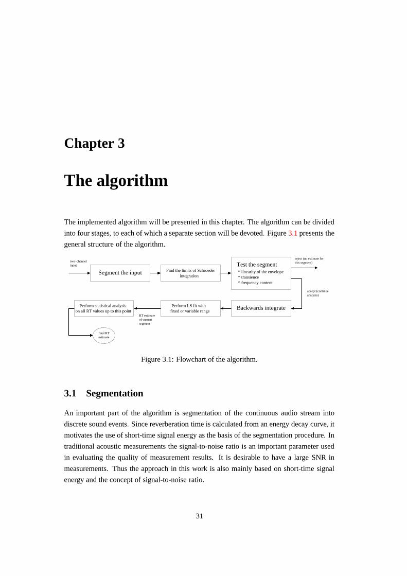
Chapter 3
The algorithm
The implemented algorithm will be presented in this chapter. The algorithm can be divided
into four stages, to each of which a separate section will be devoted. Figure 3.1 presents the
general structure of the algorithm.
RT estimateof currentsegment
final RTestimate
fixed or variable range
* linearity of the envelope* transience* frequency content
integration
inputtwo−channel
reject (no estimate forthis segment)
accept (continueanalysis)
Find the limits of SchroederTest the segment
Perform LS fit with Backwards integrate
Segment the input
on all RT values up to this pointPerform statistical analysis
Figure 3.1: Flowchart of the algorithm.
3.1 Segmentation
An important part of the algorithm is segmentation of the continuous audio stream into
discrete sound events. Since reverberation time is calculated from an energy decay curve, it
motivates the use of short-time signal energy as the basis of the segmentation procedure. In
traditional acoustic measurements the signal-to-noise ratio is an important parameter used
in evaluating the quality of measurement results. It is desirable to have a large SNR in
measurements. Thus the approach in this work is also mainly based on short-time signal
energy and the concept of signal-to-noise ratio.
31
CHAPTER 3. THE ALGORITHM 32
The segmentation procedure consists of two parts. Coarse segmentation1 is performed
first. The basic idea of the coarse segmentation algorithm is to calculate an estimate for
the mean background noise level and to detect sound event onsets whenever there is a large
enough sudden increase in signal energy. The size of required deviation from the mean can
be adjusted too meet the desired SNR requirements, since the maximum upward deviation
of short-time signal energy from the noise level can be thought as an estimate for the SNR
of a sound segment. Too low SNR will result in an unreliable estimate of the reverberation
time.
Fine segmentation follows the coarse one, giving the exact limits that will be used for
Schroeder integration (described in Section 2.3) and thus RT estimation. Each signal seg-
ment obtained as the result of coarse segmentation will be subjected to this fine-scale anal-
ysis. This part of the algorithm is the only part where the binaural nature of the signals, i.e.
the fact that two different input signals exist, is used. The interaural coherence function,
described in Section 2.5, is used for estimating the length of direct sound. The idea is that
the average of short-time coherence over frequency tells something about the diffusiveness
of an acoustical situation [63]. One could think that areas of low coherence correspond
to free decay and those of high coherence to direct sound. However, the situation is more
complicated than that, because the average coherence seems to depend on the frequency
content of the signal and the way the different frequencies are spread across time, acting as
an indicator of how transient-like a sound is (a fact that will be exploited in the estimation
algorithm). More discussion on using the coherence follows in Section 4.2.
3.1.1 Coarse segmentation
The first part of the segmentation algorithm detects interesting sound events based on
short-time energy values calculated from subsegments of length Nsub, i.e., short windowed
sequences of the signal. The length of a subsegment is typically around 50 ms. Each
subsegment sample x(n) is calculated as an average of the two channels, i.e., x(n) =
0.5(xl(n) + xr(n)). The start sample index of each subsegment is denoted by nsub. The
energy EdB of each subsegment is calculated and compared against an estimate for back-
ground noise energy level, which is the average of Nnoise latest subsegment energy values
EdB . Calculation of the noise level is implemented as a circular buffer of length Nnoise.
If the energy level of the current segment exceeds the background noise energy level by
amount Eup, a sound event is detected. When the algorithm is started, it is assumed that
the signal is background noise. It takes a few subsegments time before the algorithm gets
a good estimate for the background noise level. The background noise level estimation is
1“Sound event detection” could be also used, but it is more clear to call the entire algorithm “segmentation”,
which is divided into two parts, coarse and fine segmentation.
CHAPTER 3. THE ALGORITHM 33
naturally turned off during a sound event. It is also possible to clear the circular buffer
at this point. The end of an event is detected when the subsegment energy level falls to
Enoise + Edown or when the sound event buffer is filled completely. It is usually a good
idea to set Edown to 0 dB, because the sound event might otherwise be cut too short. The
algorithm can be presented in pseudo-code as follows:
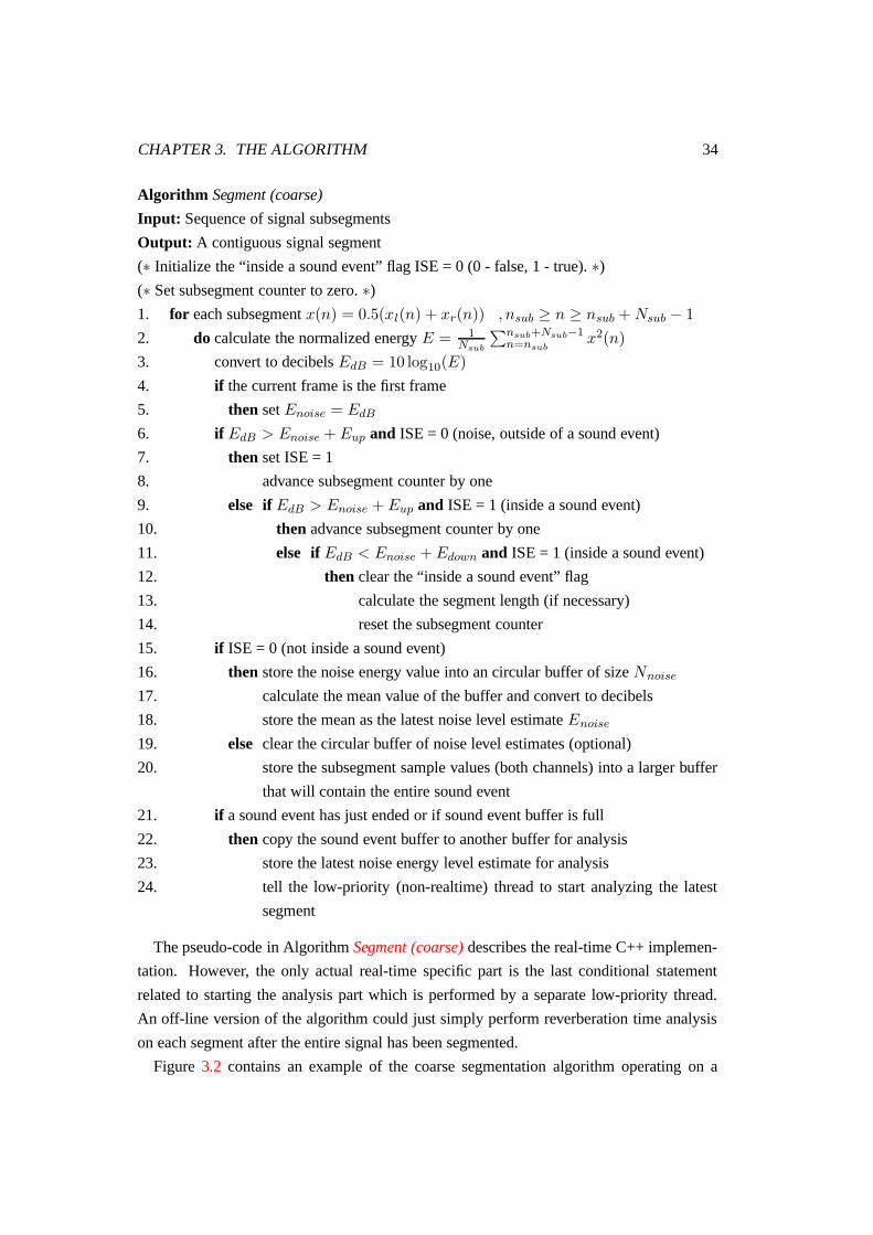
CHAPTER 3. THE ALGORITHM 34
Algorithm Segment (coarse)
Input: Sequence of signal subsegments
Output: A contiguous signal segment
(∗ Initialize the “inside a sound event” flag ISE = 0 (0 - false, 1 - true). ∗)
(∗ Set subsegment counter to zero. ∗)
1. for each subsegment x(n) = 0.5(xl(n) + xr(n)) , nsub ≥ n ≥ nsub + Nsub − 1
2. do calculate the normalized energy E = 1Nsub
∑nsub+Nsub−1n=nsub
x2(n)
3. convert to decibels EdB = 10 log10(E)
4. if the current frame is the first frame
5. then set Enoise = EdB
6. if EdB > Enoise + Eup and ISE = 0 (noise, outside of a sound event)
7. then set ISE = 1
8. advance subsegment counter by one
9. else if EdB > Enoise + Eup and ISE = 1 (inside a sound event)
10. then advance subsegment counter by one
11. else if EdB < Enoise + Edown and ISE = 1 (inside a sound event)
12. then clear the “inside a sound event” flag
13. calculate the segment length (if necessary)
14. reset the subsegment counter
15. if ISE = 0 (not inside a sound event)
16. then store the noise energy value into an circular buffer of size Nnoise
17. calculate the mean value of the buffer and convert to decibels
18. store the mean as the latest noise level estimate Enoise
19. else clear the circular buffer of noise level estimates (optional)
20. store the subsegment sample values (both channels) into a larger buffer
that will contain the entire sound event
21. if a sound event has just ended or if sound event buffer is full
22. then copy the sound event buffer to another buffer for analysis
23. store the latest noise energy level estimate for analysis
24. tell the low-priority (non-realtime) thread to start analyzing the latest
segment
The pseudo-code in Algorithm Segment (coarse) describes the real-time C++ implemen-
tation. However, the only actual real-time specific part is the last conditional statement
related to starting the analysis part which is performed by a separate low-priority thread.
An off-line version of the algorithm could just simply perform reverberation time analysis
on each segment after the entire signal has been segmented.
Figure 3.2 contains an example of the coarse segmentation algorithm operating on a
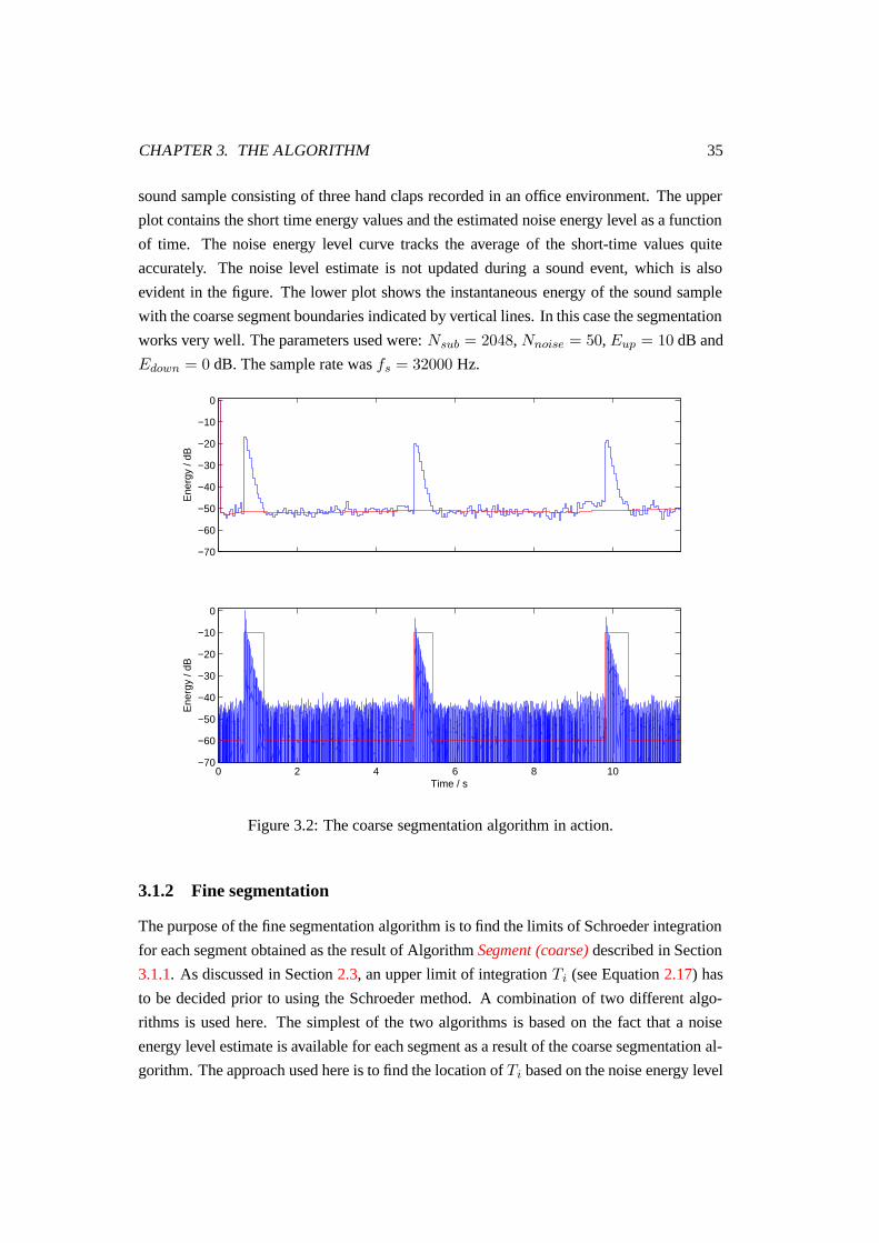
CHAPTER 3. THE ALGORITHM 35
sound sample consisting of three hand claps recorded in an office environment. The upper
plot contains the short time energy values and the estimated noise energy level as a function
of time. The noise energy level curve tracks the average of the short-time values quite
accurately. The noise level estimate is not updated during a sound event, which is also
evident in the figure. The lower plot shows the instantaneous energy of the sound sample
with the coarse segment boundaries indicated by vertical lines. In this case the segmentation
works very well. The parameters used were: Nsub = 2048, Nnoise = 50, Eup = 10 dB and
Edown = 0 dB. The sample rate was fs = 32000 Hz.
−70
−60
−50
−40
−30
−20
−10
0
Ene
rgy
/ dB
0 2 4 6 8 10−70
−60
−50
−40
−30
−20
−10
0
Ene
rgy
/ dB
Time / s
Figure 3.2: The coarse segmentation algorithm in action.
3.1.2 Fine segmentation
The purpose of the fine segmentation algorithm is to find the limits of Schroeder integration
for each segment obtained as the result of Algorithm Segment (coarse) described in Section
3.1.1. As discussed in Section 2.3, an upper limit of integration Ti (see Equation 2.17) has
to be decided prior to using the Schroeder method. A combination of two different algo-
rithms is used here. The simplest of the two algorithms is based on the fact that a noise
energy level estimate is available for each segment as a result of the coarse segmentation al-
gorithm. The approach used here is to find the location of Ti based on the noise energy level
CHAPTER 3. THE ALGORITHM 36
and energy envelope of the signal. The latter is calculated from logarithmic instantaneous
energy sequence of the signal using a standard envelope follower with different rise and fall
times, adjusted properly for this application. The resulting envelope will follow the peaks
of the instantaneous energy and can thus be used for finding Ti. The idea is to count how
many samples of the envelope are under the latest estimate for noise energy level Enoise
plus an extra marginal value Emarg , and then subtract this value from the buffer length2.
This procedure is only done from the maximum value location to the end of the buffer, be-
cause there might be low enough energy values before the maximum, causing Ti to be set
too early. It is also to be noted that in some cases Ti will be set to the end of the buffer if
there are no samples in the envelope filling the above-mentioned criterion. A pseudo code
description of the algorithm is presented in Algorithm Segment (fine).
A more complicated algorithm for location Ti is described in Section 3.1.3. This algo-
rithm requires that a part of each segment contains background noise only, i.e., the part of
the signal after the decaying sound has dived below the noise floor having almost constant
energy level. If there is too little samples of “background noise only” in the segment, the
more complicated knee point location algorithm will fail to correctly determine the inte-
gration end point (see Section 3.1.3 for more discussion). This typically happens when the
coarse segmentation algorithm sets the end of the segment to some point during the free
decay part (before diving below the noise floor). In this case Ti should be set to the very
end of the segment so that a maximal portion of the decay part is used for calculating the
integration curve. The simple algorithm for Ti usually sets Ti to the last sample of the seg-
ment in these cases, even though the extra marginal Emarg should be properly set for this
to happen. A combination of the two algorithms is therefore used for deciding the location
of Ti. If the simple algorithm gives Ti = Nseg(m), i.e., the end of the current segment, Ti
is set at the end. Otherwise the the knee point location algorithm is ran and the resulting Ti
is used. In this case there is need to truncate the segment from the end.
There is still one part of the overall algorithm belonging to the fine estimation proce-
dure: locating Td, the point up to which the decay curve is calculated using the Schroeder
method. According to [16], the direct sound and first reflections have to be excluded from
the reverberation time calculation. Td should thus be set to a location where the diffuse
sound field starts. One way of locating Td would be simply by finding the point in time
where the sound energy level falls below -5 dB from maximum. This approach is not very
accurate though, so a more sophisticated approach is taken. The coherence function, de-
scribed in Section 2.5, is used to find the length of the part of the signal containing the direct
2It is assumed that the energy envelope decays “almost monotonically” until the end of the envelope. This
is one condition that should be fulfilled if the segment contains a transient-like sound. The other conditions will
be described in Section 3.2.
CHAPTER 3. THE ALGORITHM 37
sound and possibly some early reflections (see Section 4.2 for more discussion). The use
of the coherence function is motivated by the hypothesis that the average of the short-time
coherence function (across frequency) between left and right ear signals can be used as a
measure for diffusiveness of a particular acoustic situation [63]. The interaural coherence
should thus be high during the direct sound and low during the decay. However, the short
time coherence depends on some other things as well. It can be used as an indicator of how
transient-like the direct sound is, because transient sounds have a lot of energy across a wide
range of frequencies, which in turn are concentrated around a small area in time. Thus the
short-time average coherence rises to a value close to one during a transient direct sound.
This fact will be exploited in Section 3.2 to discard unsuitable sound segments before the
actual RT analysis.
The short-time coherence function is evaluated in the fine segmentation part of the algo-
rithm, using it to find the point in time where the diffuse field starts by counting the number
of envelope samples during which the average of the short-time coherence is above a certain
threshold. The start of the diffuse sound, Td, is calculated as follows: Td = Tmax + nc,
where Tmax is the location of the maximum value of the envelope and nc is the number of
samples that are over the coherence threshold κcoh,dir. This way of calculating Td should
give a crude estimate for the point in time at which the diffuse sound starts. It should be
noted that Tmax might be at any location during the direct sound, not just at the beginning,
and thus Td might be overestimated. This is not a big issue because the system is designed
for transient sounds, which are usually not very lengthy. Overestimation is better than un-
derestimation also because underestimation will bias the integration curve upwards whereas
slight overestimation merely lowers the signal-to-noise ratio a bit.
The short-time coherence function is evaluated from overlapping windows of the entire
segment. Two NFFT point fast Fourier transforms (FFT) are calculated from each window
of length 2NFFT , one from the first NFFT samples and another from the last NFFT sam-
ples. Thus there are no overlapping samples used when calculating the two transforms from
a single window. The reason for calculating two transforms for each short-time coherence
function is that time averages have to be used when calculating coherence (see Section 2.5
and Eq. 2.25). This part is done for both channels, resulting in a total of four FFTs per
window.
The short-time coherence can alternatively be calculated using first order low-pass smooth-
ing of the spectra, as discussed in Section 2.5. The user can change the amount of smooth-
ing by adjusting the forgetting factor β. Setting β = 0 will revert into using the way of
calculating the coherence that was described before.
The algorithm can be summarized as follows:
Algorithm Segment (fine)
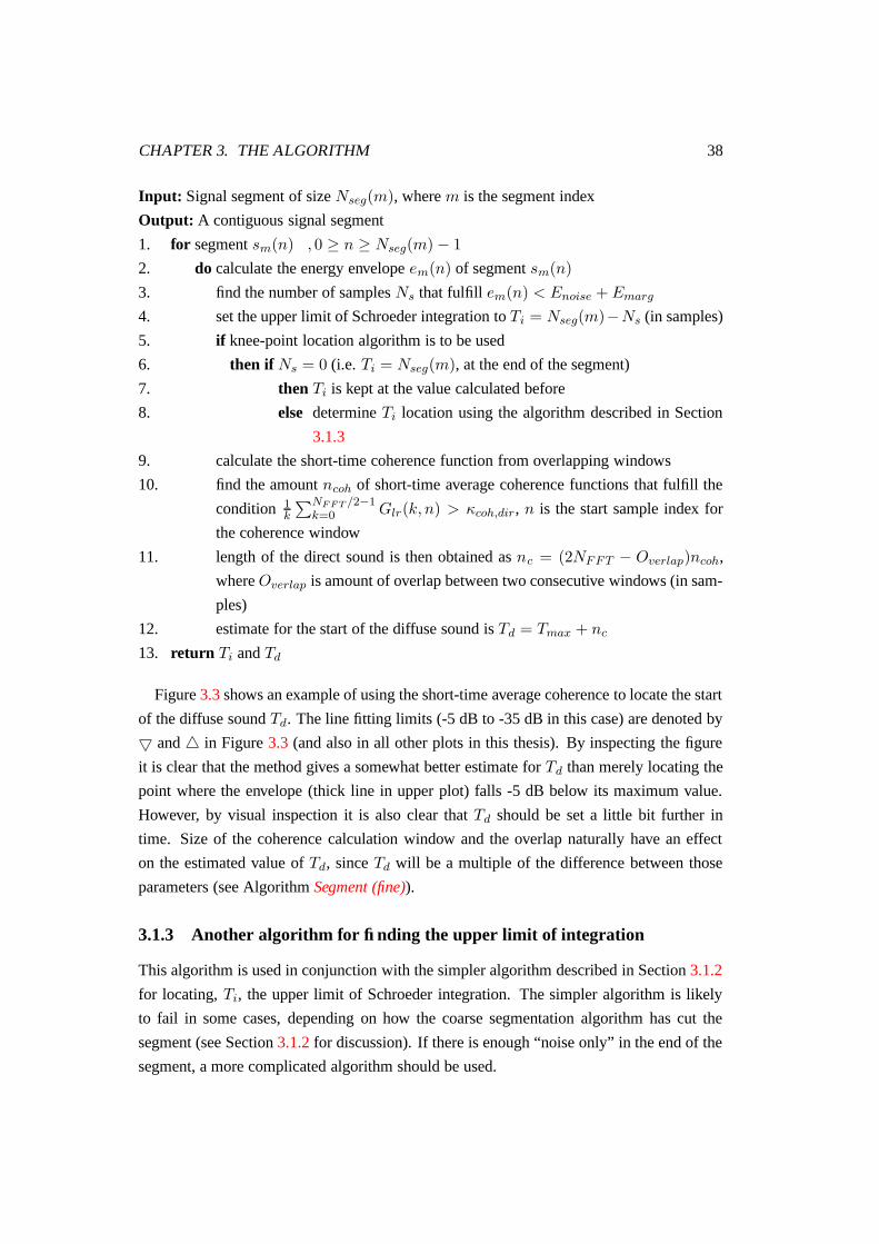
CHAPTER 3. THE ALGORITHM 38
Input: Signal segment of size Nseg(m), where m is the segment index
Output: A contiguous signal segment
1. for segment sm(n) , 0 ≥ n ≥ Nseg(m) − 1
2. do calculate the energy envelope em(n) of segment sm(n)
3. find the number of samples Ns that fulfill em(n) < Enoise + Emarg
4. set the upper limit of Schroeder integration to Ti = Nseg(m)−Ns (in samples)
5. if knee-point location algorithm is to be used
6. then if Ns = 0 (i.e. Ti = Nseg(m), at the end of the segment)
7. then Ti is kept at the value calculated before
8. else determine Ti location using the algorithm described in Section
3.1.3
9. calculate the short-time coherence function from overlapping windows
10. find the amount ncoh of short-time average coherence functions that fulfill the
condition 1k
∑NFFT /2−1k=0 Glr(k, n) > κcoh,dir, n is the start sample index for
the coherence window
11. length of the direct sound is then obtained as nc = (2NFFT − Overlap)ncoh,
where Overlap is amount of overlap between two consecutive windows (in sam-
ples)
12. estimate for the start of the diffuse sound is Td = Tmax + nc
13. return Ti and Td
Figure 3.3 shows an example of using the short-time average coherence to locate the start
of the diffuse sound Td. The line fitting limits (-5 dB to -35 dB in this case) are denoted by
5 and 4 in Figure 3.3 (and also in all other plots in this thesis). By inspecting the figure
it is clear that the method gives a somewhat better estimate for Td than merely locating the
point where the envelope (thick line in upper plot) falls -5 dB below its maximum value.
However, by visual inspection it is also clear that Td should be set a little bit further in
time. Size of the coherence calculation window and the overlap naturally have an effect
on the estimated value of Td, since Td will be a multiple of the difference between those
parameters (see Algorithm Segment (fine)).
3.1.3 Another algorithm for finding the upper limit of integration
This algorithm is used in conjunction with the simpler algorithm described in Section 3.1.2
for locating, Ti, the upper limit of Schroeder integration. The simpler algorithm is likely
to fail in some cases, depending on how the coarse segmentation algorithm has cut the
segment (see Section 3.1.2 for discussion). If there is enough “noise only” in the end of the
segment, a more complicated algorithm should be used.
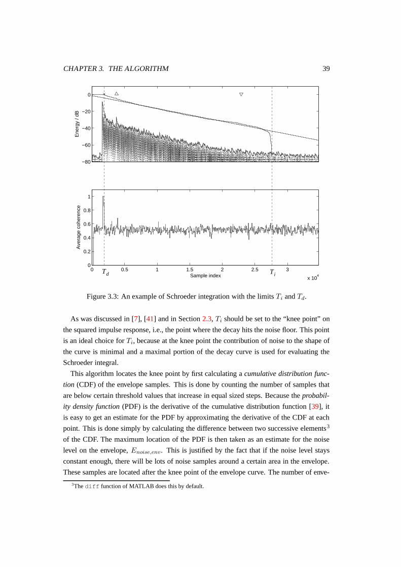
CHAPTER 3. THE ALGORITHM 39
−80
−60
−40
−20
0
Ene
rgy
/ dB
0 0.5 1 1.5 2 2.5 3
x 104
0
0.2
0.4
0.6
0.8
1
Sample index
Ave
rage
coh
eren
ce
Td T i
Figure 3.3: An example of Schroeder integration with the limits Ti and Td.
As was discussed in [7], [41] and in Section 2.3, Ti should be set to the “knee point” on
the squared impulse response, i.e., the point where the decay hits the noise floor. This point
is an ideal choice for Ti, because at the knee point the contribution of noise to the shape of
the curve is minimal and a maximal portion of the decay curve is used for evaluating the
Schroeder integral.
This algorithm locates the knee point by first calculating a cumulative distribution func-
tion (CDF) of the envelope samples. This is done by counting the number of samples that
are below certain threshold values that increase in equal sized steps. Because the probabil-
ity density function (PDF) is the derivative of the cumulative distribution function [39], it
is easy to get an estimate for the PDF by approximating the derivative of the CDF at each
point. This is done simply by calculating the difference between two successive elements3
of the CDF. The maximum location of the PDF is then taken as an estimate for the noise
level on the envelope, Enoise,env. This is justified by the fact that if the noise level stays
constant enough, there will be lots of noise samples around a certain area in the envelope.
These samples are located after the knee point of the envelope curve. The number of enve-
3The diff function of MATLAB does this by default.
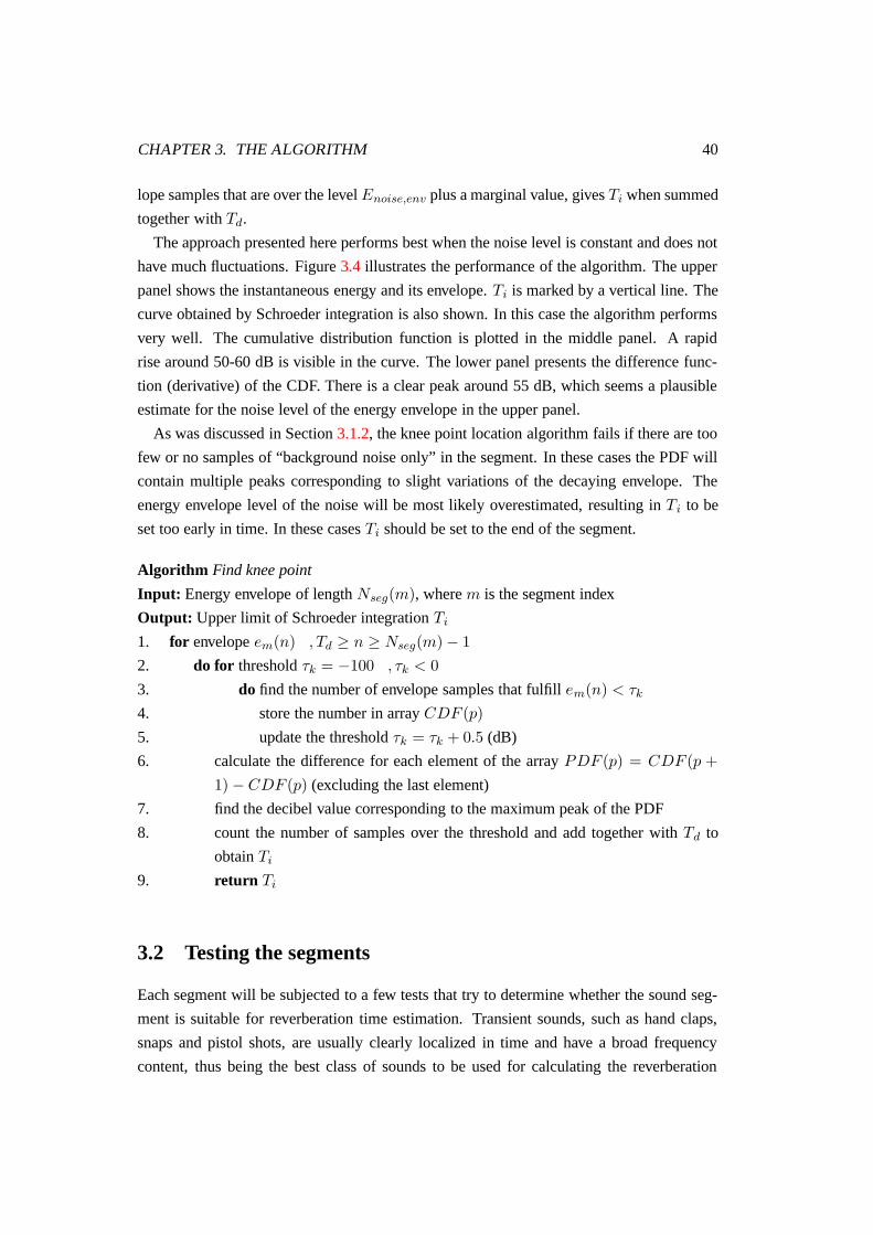
CHAPTER 3. THE ALGORITHM 40
lope samples that are over the level Enoise,env plus a marginal value, gives Ti when summed
together with Td.
The approach presented here performs best when the noise level is constant and does not
have much fluctuations. Figure 3.4 illustrates the performance of the algorithm. The upper
panel shows the instantaneous energy and its envelope. Ti is marked by a vertical line. The
curve obtained by Schroeder integration is also shown. In this case the algorithm performs
very well. The cumulative distribution function is plotted in the middle panel. A rapid
rise around 50-60 dB is visible in the curve. The lower panel presents the difference func-
tion (derivative) of the CDF. There is a clear peak around 55 dB, which seems a plausible
estimate for the noise level of the energy envelope in the upper panel.
As was discussed in Section 3.1.2, the knee point location algorithm fails if there are too
few or no samples of “background noise only” in the segment. In these cases the PDF will
contain multiple peaks corresponding to slight variations of the decaying envelope. The
energy envelope level of the noise will be most likely overestimated, resulting in Ti to be
set too early in time. In these cases Ti should be set to the end of the segment.
Algorithm Find knee point
Input: Energy envelope of length Nseg(m), where m is the segment index
Output: Upper limit of Schroeder integration Ti
1. for envelope em(n) , Td ≥ n ≥ Nseg(m) − 1
2. do for threshold τk = −100 , τk < 0
3. do find the number of envelope samples that fulfill em(n) < τk
4. store the number in array CDF (p)
5. update the threshold τk = τk + 0.5 (dB)
6. calculate the difference for each element of the array PDF (p) = CDF (p +
1) − CDF (p) (excluding the last element)
7. find the decibel value corresponding to the maximum peak of the PDF
8. count the number of samples over the threshold and add together with Td to
obtain Ti
9. return Ti
3.2 Testing the segments
Each segment will be subjected to a few tests that try to determine whether the sound seg-
ment is suitable for reverberation time estimation. Transient sounds, such as hand claps,
snaps and pistol shots, are usually clearly localized in time and have a broad frequency
content, thus being the best class of sounds to be used for calculating the reverberation
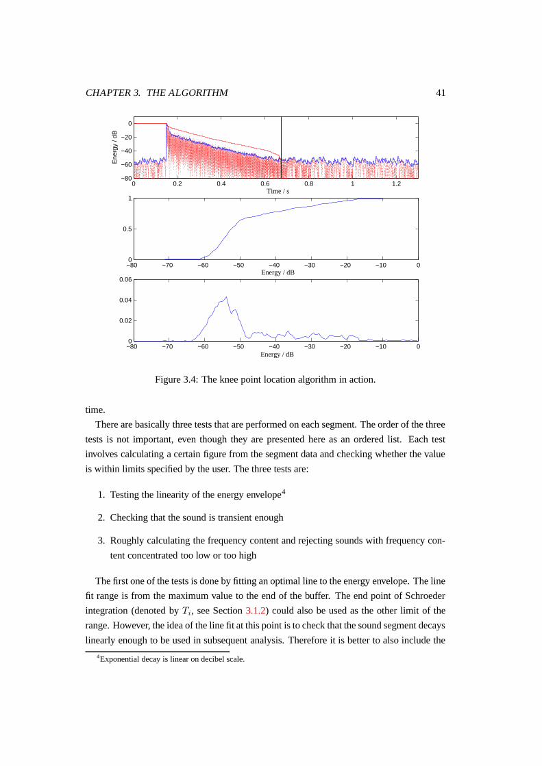
CHAPTER 3. THE ALGORITHM 41
0 0.2 0.4 0.6 0.8 1 1.2−80
−60
−40
−20
0
Ene
rgy
/ dB
−80 −70 −60 −50 −40 −30 −20 −10 00
0.5
1
−80 −70 −60 −50 −40 −30 −20 −10 00
0.02
0.04
0.06
Time / s
Energy / dB
Energy / dB
Figure 3.4: The knee point location algorithm in action.
time.
There are basically three tests that are performed on each segment. The order of the three
tests is not important, even though they are presented here as an ordered list. Each test
involves calculating a certain figure from the segment data and checking whether the value
is within limits specified by the user. The three tests are:
1. Testing the linearity of the energy envelope4
2. Checking that the sound is transient enough
3. Roughly calculating the frequency content and rejecting sounds with frequency con-
tent concentrated too low or too high
The first one of the tests is done by fitting an optimal line to the energy envelope. The line
fit range is from the maximum value to the end of the buffer. The end point of Schroeder
integration (denoted by Ti, see Section 3.1.2) could also be used as the other limit of the
range. However, the idea of the line fit at this point is to check that the sound segment decays
linearly enough to be used in subsequent analysis. Therefore it is better to also include the
4Exponential decay is linear on decibel scale.
CHAPTER 3. THE ALGORITHM 42
end of the buffer for this check, since something might happen after Ti, indicating that the
current segment is not very suitable for reverberation time analysis. This is intended to
be a very coarse check to make sure that there is nothing strange happening in the current
segment. A value for correlation coefficient of line fitting as low as 0.8 could be used.
The motivation behind the second test is the fact that transient sounds, such as hand
claps, have desirable properties for reverberation time estimation. Transient sounds usually
have their frequency content concentrated around a small time window, which in turn raises
the short-time average coherence. The test involves further inspection of the short-time
average coherence that was calculated in Algorithm Segment (fine) (Section 3.1.2). The
maximum value of the short-time coherence is compared against a user-definable threshold
value κcoh,max5. If the maximum value is below the threshold, the segment is discarded.
The reverberation time varies as a function of frequency and since arbitrary sounds may
have arbitrary frequency content, the frequency content of each sound segment has to be
taken into account. If a single figure, the reverberation time T60, is given, it is usually
assumed to be calculated on the octave band centered at 500 Hz (see Section 2.2.1). Sound
segments that have considerable frequency content at lower and higher frequencies should
thus be excluded from the reverberation time analysis. This is done by first calculating the
spectral centroid defined in Section 2.6. The spectral centroid is calculated from a single
window starting from the maximum value of the energy envelope. If the centroid value is
outside a frequency band specified by the user, the sound event is discarded. The spectral
centroid is a very rough measure of the frequency content of a signal, but quite adequate
for this application, since the idea is to simply rule out extreme cases, especially sounds
that have substantial low frequency content. Another way of getting rid of low-frequency
segments could be high-pass filtering of the signal prior to analysis. The cut-off frequency
could be somewhere around 100 Hz.
3.3 Estimation of RT
This part of the overall algorithm is quite straightforward and relies on the well-known
Schroeder method (see Section 2.3) and the least squares method for line fitting (see Section
2.4). The Schroeder integral is calculated from the instantaneous squared signal for a range
of Td to Ti. The integration curve is normalized to have its maximum value at 0 dB. This
is done by subtracting the maximum value from the curve. Line fitting is then performed
on the normalized integration curve. There is just one important decision related to the
least squares fit, namely the range of the integration curve that the line is fitted to. A
simple choice would be a fixed range, -5 to -25 dB or alternatively -5 to -35 dB. There is a
5This is not the same threshold that was used in locating the end of direct sound in Section 3.1.2.
CHAPTER 3. THE ALGORITHM 43
problem with the fixed range approach though. A bias might be introduced to the slope of
the fitted line at either end of the integration curve. This is a big problem especially with
uncontrolled excitation signals, when nothing can be done to improve the signal-to-noise
ratio. An algorithm (or rule) for finding the range of line fitting was developed as part of
this work (see Section 3.3.1).
The reverberation time T60 itself is calculated from the slope of the fitted line by a very
simple formula:
T60 = −60
b
1
fs, b < 0 (3.1)
where b is the slope of the fitted line and fs is the sampling frequency.
3.3.1 Finding the limits for line fitting
The limits of the least squares fit are important for accurateness of the RT estimates. Even
a small bending of the integration curve may strongly affect the slope of the fitted line and
the RT calculated based on the slope. The lower limit for line fit6 is especially important,
since the Schroeder integration curve always bends down at the end. If the integration is
started too far in time, i.e., during the background noise, the integration curve will be bent
upwards at the end, making RT to be overestimated. It would be advantageous to do the line
fitting to a part of the integration curve that is as linear as possible, yet having a maximal
portion of the curve to be included in the fitting.
One possible solution is based on doing the line fitting multiple times, moving the lower
limit from the end (or -25 / -35 dB) towards the -5 dB point, at which the other limit of
line fit is kept fixed. A small marginal is left near the -5 dB point, since the least squares fit
becomes very noisy in this application when the data record is too short. Obviously there
is no point in doing the line fitting for just a couple of integration curve samples. The end
point is moved after each least squares fit calculation and T60 is calculated from the slope
of the line b (using Equation 3.1). Finally the correlation coefficient r2 is stored in an array.
It is hypothesized that the best reverberation time estimate could be found by locating the
maximum of the r2 curve and picking the T60 from the same location in time.
Figure 3.5 shows the RT (middle panel) and correlation coefficient (lower panel) plotted
as a function of the location of the rightmost line fitting limit. The rightmost limit of line
fitting starts from -35 dB and moves with hops of 40 samples towards the -5 dB point,
leaving a 100 sample marginal. It seems that a good choice for the rightmost limit of line
fitting would be at the point where the correlation coefficient reaches its maximum value
(marked by ’x’ in the figures). The effect of downward bending of the integration curve is
6The one that is further in time.
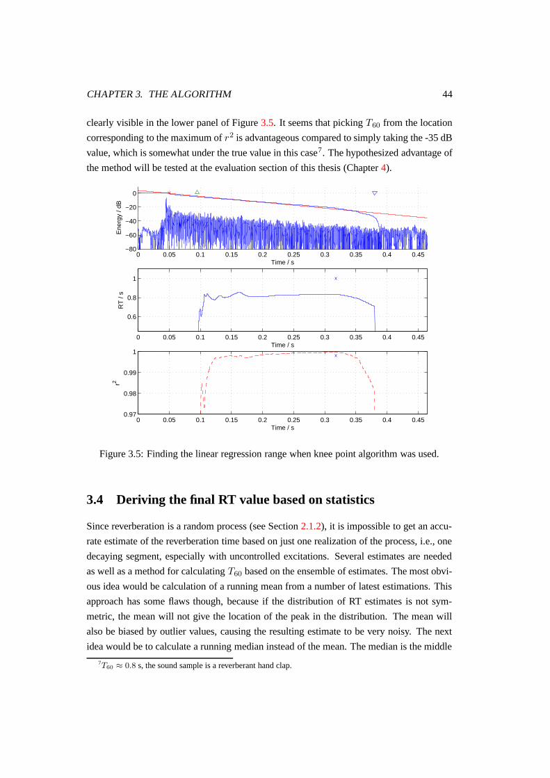
CHAPTER 3. THE ALGORITHM 44
clearly visible in the lower panel of Figure 3.5. It seems that picking T60 from the location
corresponding to the maximum of r2 is advantageous compared to simply taking the -35 dB
value, which is somewhat under the true value in this case7. The hypothesized advantage of
the method will be tested at the evaluation section of this thesis (Chapter 4).
0 0.05 0.1 0.15 0.2 0.25 0.3 0.35 0.4 0.45−80
−60
−40
−20
0
Ene
rgy
/ dB
Time / s
0 0.05 0.1 0.15 0.2 0.25 0.3 0.35 0.4 0.45
0.6
0.8
1
RT
/ s
Time / s
0 0.05 0.1 0.15 0.2 0.25 0.3 0.35 0.4 0.450.97
0.98
0.99
1
r2
Time / s
Figure 3.5: Finding the linear regression range when knee point algorithm was used.
3.4 Deriving the final RT value based on statistics
Since reverberation is a random process (see Section 2.1.2), it is impossible to get an accu-
rate estimate of the reverberation time based on just one realization of the process, i.e., one
decaying segment, especially with uncontrolled excitations. Several estimates are needed
as well as a method for calculating T60 based on the ensemble of estimates. The most obvi-
ous idea would be calculation of a running mean from a number of latest estimations. This
approach has some flaws though, because if the distribution of RT estimates is not sym-
metric, the mean will not give the location of the peak in the distribution. The mean will
also be biased by outlier values, causing the resulting estimate to be very noisy. The next
idea would be to calculate a running median instead of the mean. The median is the middle
7T60 ≈ 0.8 s, the sound sample is a reverberant hand clap.
CHAPTER 3. THE ALGORITHM 45
value after ordering a number of samples, i.e, 50 % of the distribution will be below the
median. For perfectly Gaussian distributions the median will be equal to the mean, giving
the peak location in the distribution (or probability density function).
The running median and the running mean are actually special cases of an order statistics
filter8 (OSF) [4]. The mean is a purely linear operation while the median is non-linear,
moving to the area of non-linear filtering [27]. A general order statistics filter gives out
a linear combination of ordered sample values. If only the middle value is given out, the
resulting filter is the median filter. Ratnam et al. [49] [48] use an order statistics filter
to derive the final RT estimate from a histogram of estimates using an order statistics filter.
They propose two different strategies to be used in different situations. One idea is to output
a value that limits 10 % of the histogram (distribution) values below itself. The other idea
is also motivated by the histogram of estimates and is not actually an order statistics filter.
The idea is to choose the RT value corresponding to the lowest peak in the histogram. This
is also very suitable for the current algorithm, because unlike in the algorithm proposed by
Ratnam et al., the estimates are only calculated from the parts of the signal with free decay,
provided that the checks in Section 3.2 do not fail. No estimate is calculated from other
parts and the histogram should thus have a clear peak close to the true RT value. Due to the
statistical nature of reverberation and the fact that the incoming signal is arbitrary, it will
take a few estimates before a prominent peak will appear in the histogram.
It is also possible to set a forgetting factor αh ∈ ]0, 1] to create a “fading” histogram.
After a new estimate is calculated and the corresponding histogram bin value is accumu-
lated by one, each histogram bin is multiplied by αh. The motivation behind the fading
histogram is that when the user moves into another room, the new RT will be picked up by
the algorithm sooner, thanks to the decreasing RT peak of the previous room. The value of
αh is typically a little bit below one. If αh = 1, the histogram remains untouched after each
new estimate is added.
3.5 Implementation of the algorithm
An initial version of the algorithm was first written for MATLAB. The MATLAB imple-
mentation was then translated to a real-time implementation in C++ using the Mustajuuri
[21] framework. The real-time algorithm uses threads [57] to divide the computational bur-
den over time. A real-time DSP thread is responsible for collecting samples to buffers and
locating sound events based on short-time energy calculations (more detailed discussion in
Section 3.1). The latter process will be termed “segmentation” (see Section 2.7 for more
discussion). After the end point of a sound segment is decided, the corresponding segment
8Also known as L-filter [27]
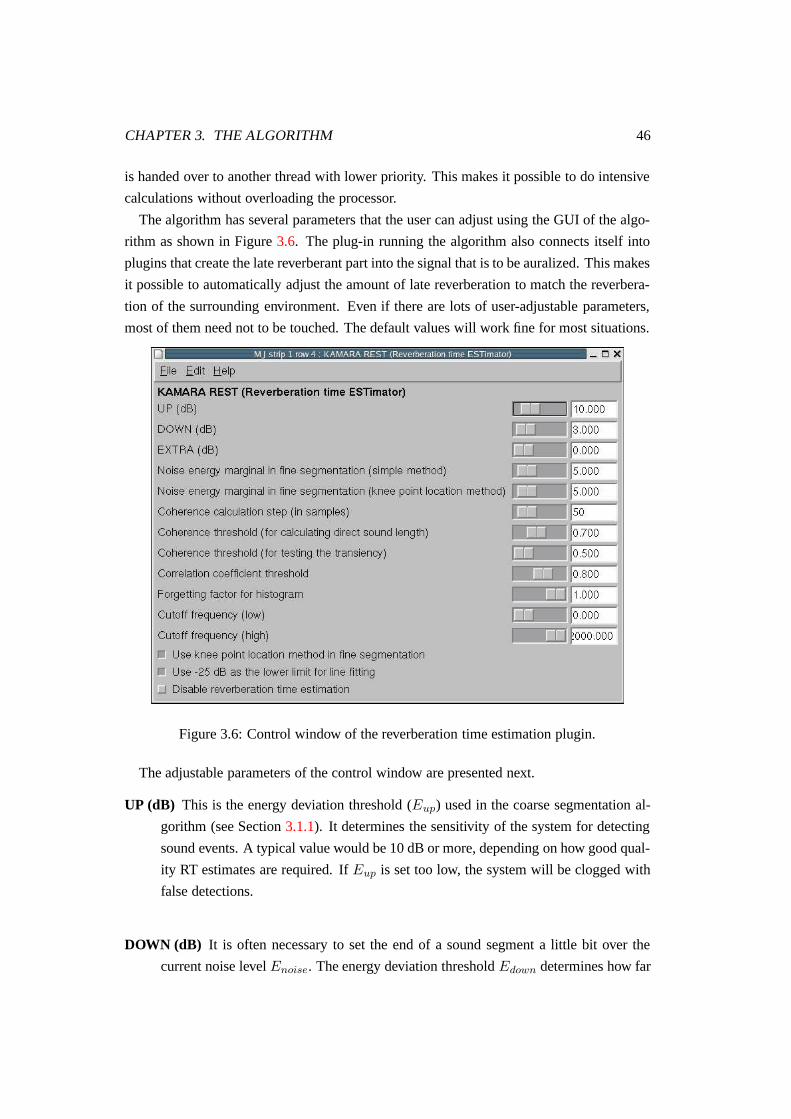
CHAPTER 3. THE ALGORITHM 46
is handed over to another thread with lower priority. This makes it possible to do intensive
calculations without overloading the processor.
The algorithm has several parameters that the user can adjust using the GUI of the algo-
rithm as shown in Figure 3.6. The plug-in running the algorithm also connects itself into
plugins that create the late reverberant part into the signal that is to be auralized. This makes
it possible to automatically adjust the amount of late reverberation to match the reverbera-
tion of the surrounding environment. Even if there are lots of user-adjustable parameters,
most of them need not to be touched. The default values will work fine for most situations.
Figure 3.6: Control window of the reverberation time estimation plugin.
The adjustable parameters of the control window are presented next.
UP (dB) This is the energy deviation threshold (Eup) used in the coarse segmentation al-
gorithm (see Section 3.1.1). It determines the sensitivity of the system for detecting
sound events. A typical value would be 10 dB or more, depending on how good qual-
ity RT estimates are required. If Eup is set too low, the system will be clogged with
false detections.
DOWN (dB) It is often necessary to set the end of a sound segment a little bit over the
current noise level Enoise. The energy deviation threshold Edown determines how far
CHAPTER 3. THE ALGORITHM 47
into the decay the coarse segmentation algorithm sets the end of the segment. A too
low value will cause too much noise to be left into the segments, while a too high
value will cut the segment too early. A good choice for Edown would be around 2-5
decibels.
EXTRA (dB) If a high SNR and good quality estimates are desired, it might be advanta-
geous to analyze only those sound segments that have a large upward deviation from
the noise mean, yet excluding segments with lower SNR from calculating the noise
level. By adjusting this parameter to a value greater than zero, only segments that
have an onset of more than Eup + Eextra decibels will be included in reverberation
time analysis. Segments with onset greater than Eup will be excluded from the noise
level calculation but not included in RT analysis, i.e., the low-priority thread is not
started.
Noise energy marginal in fine segmentation (simple method) When the simple fine seg-
mentation method, described in Section 3.1.2, is used for determining the truncation
point Ti, an energy threshold little bit greater than the noise mean is needed. In prac-
tice, this marginal (Emarg) determines how far into the decay Ti is set. A typical
value for this parameter would be around 1-5 dB.
Noise energy marginal in fine segmentation (knee point location method) This is the sa-
me parameter as the previous one with the exception that this one is used in the more
advanced knee point location method described in Section 3.1.3. It is thus possible to
adjust the marginals of the two algorithms separately. This parameter is also usually
set around 1-5 dB.
Coherence calculation step (in samples) This is the window “hop” size for calculating
the short-time coherence of each signal segment. A too high value will cause the av-
erage coherence to be too coarse over time, whereas a too low value will most likely
clog the system, as the calculation will take too much time. A typical value for this
parameter is around 50 (samples).
Coherence threshold (for locating the start of diffuse sound) In Section 3.1.2 it was hy-
pothesized that the average of short-time coherence could be used to find the start
point of the diffuse sound and thus the point onwards from which the reverberation
CHAPTER 3. THE ALGORITHM 48
time would be evaluated. This parameter controls κcoh,dir, a threshold value for the
average short-time coherence. The start of diffuse sound is located based on the av-
erage coherence being higher during the direct sound and reflections. A typical value
for this threshold would be around 0.7 - 0.9. It is generally better to set this threshold
into a high enough value.
Coherence threshold (for testing transience) There is a clear peak in the average short-
time coherence for transient sounds. By thresholding the maximum value of the av-
erage short-time coherence for a given sound segment, the sounds that are “transient
enough” can be detected. A typical value for this parameter would be around 0.8 -
0.9. Setting this parameter to 0.5 effectively turns the transiency check off, since for
diffuse, non-correlating sound segments the average coherence over frequency will
fluctuate around 0.5, so there is always one value that is equal or greater than 0.5.
Correlation coefficient threshold Each segment is tested for anomalities in the energy
envelope shape, as described in Section 3.2. The idea is to rule out very nonlinearly
shaped envelopes, indicating that there is not well-behaving linear decay in the cur-
rent sound segment. A sound segment is totally useless for RT evaluation if there
is no exponential decay9 present in the energy envelope. This parameter would be
typically set to a value around 0.8, effectively ruling out the most pathological cases.
Forgetting factor for histogram It is possible to get a fading histogram by setting this
value to less than one. The histogram values are multiplied by the forgetting factor
after each new estimate has arrived, i.e., the corresponding histogram bin value is
accumulated by one. A typical value for the forgetting factor would be greater than
0.9. Setting the forgetting factor to one effectively results in a normal, non-fading
histogram.
Lower limit for spectral centroid (in Hz) The frequency content of the binaural signals
should somehow be taken into account, since reverberation time of an acoustic space
is more or less frequency dependent. This algorithm approaches the problem by dis-
carding segments that have their energy concentrated too high or too low (see Section
3.2). The spectral centroid, described in Section 2.6, is calculated from a signal win-
dow starting at the maximum value of the buffer (which is roughly close to the start
9Exponential decay is linear on a logarithmic scale.
CHAPTER 3. THE ALGORITHM 49
of the direct sound). This parameter gives the lower limit for acceptable value of
the spectral centroid in Hz. If the spectral centroid of a given segment is below this
lower limit, the segment is excluded from subsequent analysis. A typical value for
this parameter could be around 300-500 Hz.
Upper limit for spectral centroid (in Hz) This is the upper limit for spectral centroid (see
discussion above), typically set around 5 kHz.
Use knee point location method in fine segmentation If checked, the more complicated
algorithm for locating the upper limit of Schroeder integration (Ti) will be used (see
Section 3.1.3).
Use -25 dB as the lower limit for line fitting If checked, -25 decibels will be used as the
lower limit in the least squares calculations (see Section 2.4). Otherwise -35 dB will
be used. It should be noted that the algorithm that searches for the optimal linear
regression range (see Section 3.3.1) will use the same lower limit as a starting point,
if activated.
Disable reverberation time estimation Checking this box will disable the RT estimation,
i.e., the low-priority thread is not started. The coarse segmentation and noise level
estimation will keep on running.
Chapter 4
Evaluation
This chapter is devoted to the evaluation of the implemented algorithm. Some basic proper-
ties of the algorithm are tested first using synthetic excitation signals. The algorithm is also
tested with more realistic signals by convolving an anechoic recording with binaural room
impulse responses measured from a few different spaces.
It is important to verify the basic functionality of the algorithm. The first part of evalua-
tion uses simple artificial signals to check that the algorithm estimates the decay correctly.
Test signals of systematically varied frequency content are fed into the system to get an idea
of how the frequency content affects the estimation results. Short time coherence plots are
also investigated to see how the frequency content of the input signal affects the average of
the coherence and whether the coherence actually can be helpful in discriminating between
the direct sound/reflections and the diffuse tail.
Moving towards more realistic usage of the algorithm, the next part of evaluation con-
sists of convolving anechoic source signals with binaural room impulse responses (BRIRs)
measured from different rooms. This part of evaluation is quite similar to the part with
synthetic signals. The purpose is to verify that the algorithm also works with non-synthetic
signals.
The true performance of the algorithm is what really counts. That is why the algorithm
is also evaluated by using realistic signals, simulating a real usage situation. The binaural
signals from microphones worn by the user are recorded using a portable hard-disk recorder.
4.1 The signals and impulse responses used in evaluation
In order to test the algorithm, some monophonic anechoic source signals and binaural room
impulse responses are needed to compose the test signals. The author made a few record-
ings in the small anechoic chamber of the HUT Laboratory of Acoustics and Audio Signal
50
CHAPTER 4. EVALUATION 51
Processing1 . The recordings consisted of hand claps, finger snaps and some miscellaneous
utterances, all performed by the author.
Binaural room impulse responses were obtained by various methods. The author mea-
sured one of the responses from an office space (A152). Another impulse response of a
small lecture hall (T3) was provided courtesy of a colleague of the author and yet another
one (Pergola) was obtained from the Ramsete web site2. Thus a total of three different
binaural room impulse responses were used for the evaluation. All responses have rever-
beration times differing by more than approximately 200 milliseconds. All BRIRs were
processed by a method proposed in [22] in order to extend the reverberant decay below the
original noise floor. This is necessary for good quality auralization.
The true reverberation times were measured from each response by the standard Schroeder
method with the integration limits chosen by manual inspection. The objective was not to
get a very high quality estimate for the RT, but a “close enough” value. A high quality
RT estimate would have required several impulse response measurements. Results of the
manual reverberation time evaluation can be found from the in Table 4.1. The evaluation
ranges were also given. The range of T3 is five decibels shorter, because the poor SNR did
not allow evaluation up to -35 dB. The response measured from A152 has the best SNR,
thanks to the sweep measurement method (see Section 2.11.2).
The BRIR of the author’s office room was calculated as follows. A Genelec3 monitor
speaker was fed with a logarithmic sine sweep of length 3 seconds plus 2 seconds of silence.
The same amount of data was simultaneously recorded by using a custom-made headset (see
Section 1.1) worn by a user located approximately two meters from the speaker. Using the
acquired data, the BRIR was obtained by frequency domain division H(z) = Y (z)/X(z),
which is also the frequency-domain definition of transfer function. The method used for
measuring the BRIR did not include compensating for non-idealities in the measurement
chain, as described in a tutorial paper on sweep measurements by Müller and Massarani
[42]. Sweep method was chosen, because it gives a better signal-to-noise ratio than MLS
and is also easier to implement [42]. An estimate for the true reverberation time was calcu-
lated by Schroeder integration and line fitting. The integration limits Td and Ti (see Section
3.1.2) were chosen by hand. The procedure was performed for both channels and the final
T60 value was derived as the mean between the two channels. The same method was used
for determining the approximate true RTs of the two other responses (see Table 4.1).
1http://www.acoustics.hut.fi2http://www.ramsete.com/Public/Aurora_CD/RoomIR/3http://www.genelec.com
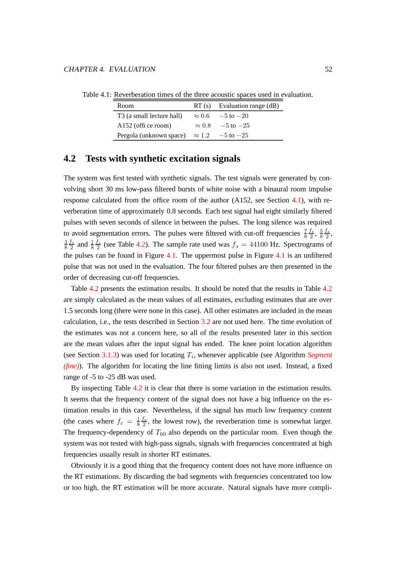
CHAPTER 4. EVALUATION 52
Table 4.1: Reverberation times of the three acoustic spaces used in evaluation.
Room RT (s) Evaluation range (dB)
T3 (a small lecture hall) ≈ 0.6 −5 to −20
A152 (office room) ≈ 0.8 −5 to −25
Pergola (unknown space) ≈ 1.2 −5 to −25
4.2 Tests with synthetic excitation signals
The system was first tested with synthetic signals. The test signals were generated by con-
volving short 30 ms low-pass filtered bursts of white noise with a binaural room impulse
response calculated from the office room of the author (A152, see Section 4.1), with re-
verberation time of approximately 0.8 seconds. Each test signal had eight similarly filtered
pulses with seven seconds of silence in between the pulses. The long silence was required
to avoid segmentation errors. The pulses were filtered with cut-off frequencies 78
fs
2 , 58
fs
2 ,38
fs
2 and 18
fs
2 (see Table 4.2). The sample rate used was fs = 44100 Hz. Spectrograms of
the pulses can be found in Figure 4.1. The uppermost pulse in Figure 4.1 is an unfiltered
pulse that was not used in the evaluation. The four filtered pulses are then presented in the
order of decreasing cut-off frequencies.
Table 4.2 presents the estimation results. It should be noted that the results in Table 4.2
are simply calculated as the mean values of all estimates, excluding estimates that are over
1.5 seconds long (there were none in this case). All other estimates are included in the mean
calculation, i.e., the tests described in Section 3.2 are not used here. The time evolution of
the estimates was not a concern here, so all of the results presented later in this section
are the mean values after the input signal has ended. The knee point location algorithm
(see Section 3.1.3) was used for locating Ti, whenever applicable (see Algorithm Segment
(fine)). The algorithm for locating the line fitting limits is also not used. Instead, a fixed
range of -5 to -25 dB was used.
By inspecting Table 4.2 it is clear that there is some variation in the estimation results.
It seems that the frequency content of the signal does not have a big influence on the es-
timation results in this case. Nevertheless, if the signal has much low frequency content
(the cases where fc = 18
fs
2 , the lowest row), the reverberation time is somewhat larger.
The frequency-dependency of T60 also depends on the particular room. Even though the
system was not tested with high-pass signals, signals with frequencies concentrated at high
frequencies usually result in shorter RT estimates.
Obviously it is a good thing that the frequency content does not have more influence on
the RT estimations. By discarding the bad segments with frequencies concentrated too low
or too high, the RT estimation will be more accurate. Natural signals have more compli-
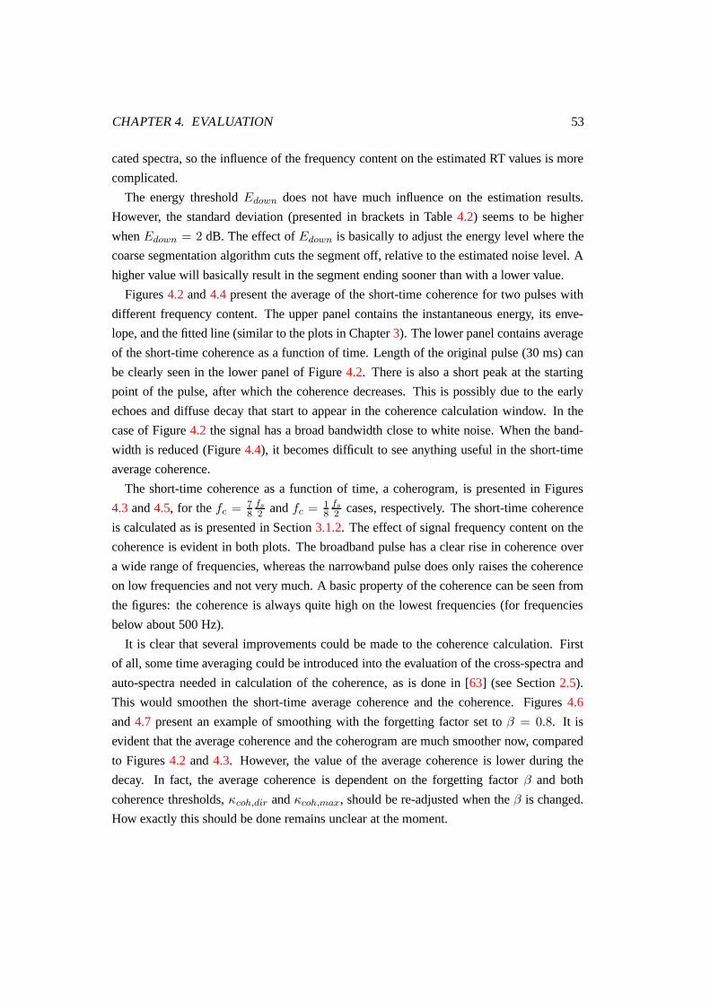
CHAPTER 4. EVALUATION 53
cated spectra, so the influence of the frequency content on the estimated RT values is more
complicated.
The energy threshold Edown does not have much influence on the estimation results.
However, the standard deviation (presented in brackets in Table 4.2) seems to be higher
when Edown = 2 dB. The effect of Edown is basically to adjust the energy level where the
coarse segmentation algorithm cuts the segment off, relative to the estimated noise level. A
higher value will basically result in the segment ending sooner than with a lower value.
Figures 4.2 and 4.4 present the average of the short-time coherence for two pulses with
different frequency content. The upper panel contains the instantaneous energy, its enve-
lope, and the fitted line (similar to the plots in Chapter 3). The lower panel contains average
of the short-time coherence as a function of time. Length of the original pulse (30 ms) can
be clearly seen in the lower panel of Figure 4.2. There is also a short peak at the starting
point of the pulse, after which the coherence decreases. This is possibly due to the early
echoes and diffuse decay that start to appear in the coherence calculation window. In the
case of Figure 4.2 the signal has a broad bandwidth close to white noise. When the band-
width is reduced (Figure 4.4), it becomes difficult to see anything useful in the short-time
average coherence.
The short-time coherence as a function of time, a coherogram, is presented in Figures
4.3 and 4.5, for the fc = 78
fs
2 and fc = 18
fs
2 cases, respectively. The short-time coherence
is calculated as is presented in Section 3.1.2. The effect of signal frequency content on the
coherence is evident in both plots. The broadband pulse has a clear rise in coherence over
a wide range of frequencies, whereas the narrowband pulse does only raises the coherence
on low frequencies and not very much. A basic property of the coherence can be seen from
the figures: the coherence is always quite high on the lowest frequencies (for frequencies
below about 500 Hz).
It is clear that several improvements could be made to the coherence calculation. First
of all, some time averaging could be introduced into the evaluation of the cross-spectra and
auto-spectra needed in calculation of the coherence, as is done in [63] (see Section 2.5).
This would smoothen the short-time average coherence and the coherence. Figures 4.6
and 4.7 present an example of smoothing with the forgetting factor set to β = 0.8. It is
evident that the average coherence and the coherogram are much smoother now, compared
to Figures 4.2 and 4.3. However, the value of the average coherence is lower during the
decay. In fact, the average coherence is dependent on the forgetting factor β and both
coherence thresholds, κcoh,dir and κcoh,max, should be re-adjusted when the β is changed.
How exactly this should be done remains unclear at the moment.
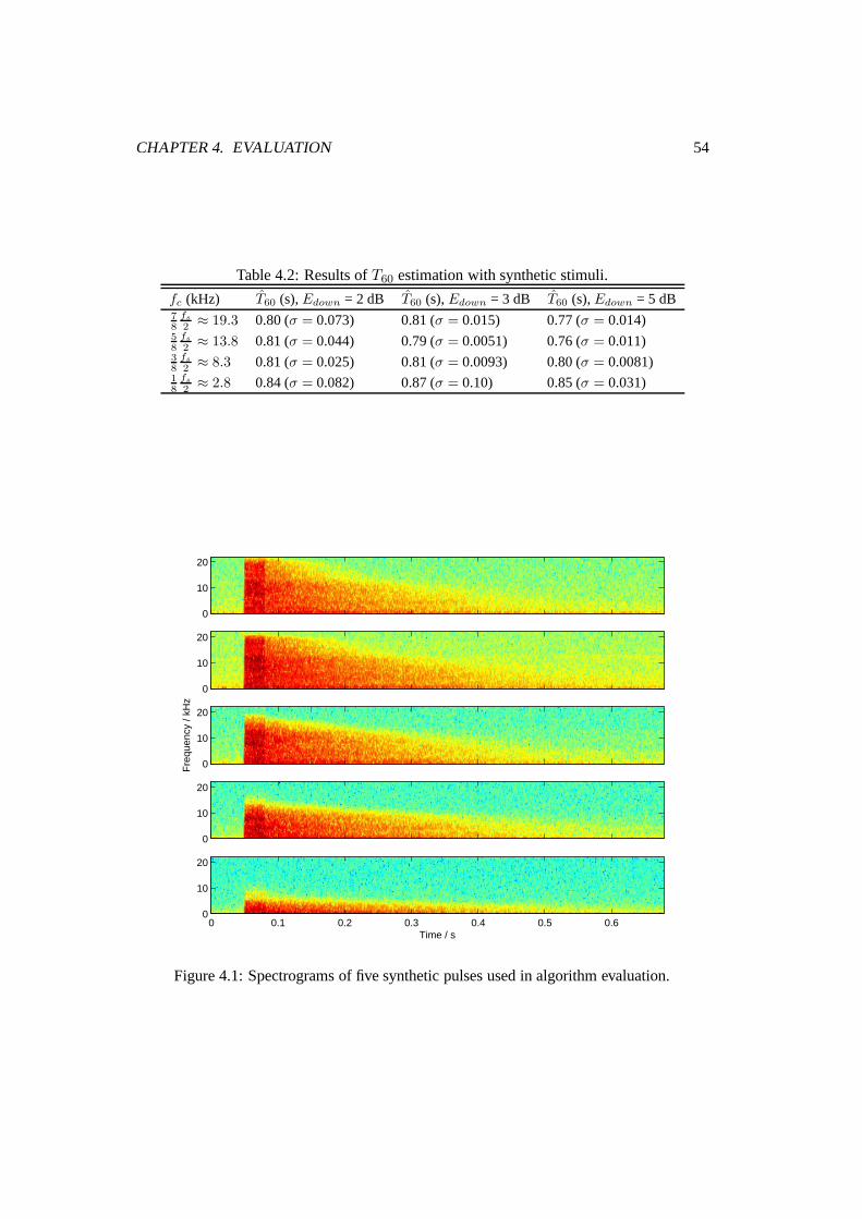
CHAPTER 4. EVALUATION 54
Table 4.2: Results of T60 estimation with synthetic stimuli.
fc (kHz) T60 (s), Edown = 2 dB T60 (s), Edown = 3 dB T60 (s), Edown = 5 dB7
8
fs
2≈ 19.3 0.80 (σ = 0.073) 0.81 (σ = 0.015) 0.77 (σ = 0.014)
5
8
fs
2≈ 13.8 0.81 (σ = 0.044) 0.79 (σ = 0.0051) 0.76 (σ = 0.011)
3
8
fs
2≈ 8.3 0.81 (σ = 0.025) 0.81 (σ = 0.0093) 0.80 (σ = 0.0081)
1
8
fs
2≈ 2.8 0.84 (σ = 0.082) 0.87 (σ = 0.10) 0.85 (σ = 0.031)
0
10
20
0
10
20
Fre
quen
cy /
kHz
0
10
20
0
10
20
Time / s0 0.1 0.2 0.3 0.4 0.5 0.6
0
10
20
Figure 4.1: Spectrograms of five synthetic pulses used in algorithm evaluation.
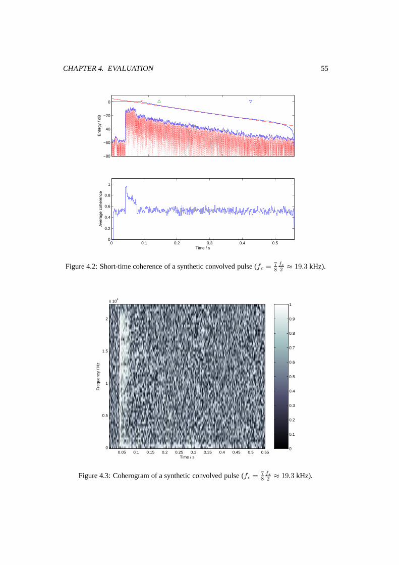
CHAPTER 4. EVALUATION 55
−80
−60
−40
−20
0E
nerg
y / d
B
0 0.1 0.2 0.3 0.4 0.50
0.2
0.4
0.6
0.8
1
Time / s
Ave
rage
coh
eren
ce
Figure 4.2: Short-time coherence of a synthetic convolved pulse (fc = 78
fs
2 ≈ 19.3 kHz).
Time / s
Fre
quen
cy /
Hz
0.05 0.1 0.15 0.2 0.25 0.3 0.35 0.4 0.45 0.5 0.550
0.5
1
1.5
2
x 104
0
0.1
0.2
0.3
0.4
0.5
0.6
0.7
0.8
0.9
1
Figure 4.3: Coherogram of a synthetic convolved pulse (fc = 78
fs
2 ≈ 19.3 kHz).
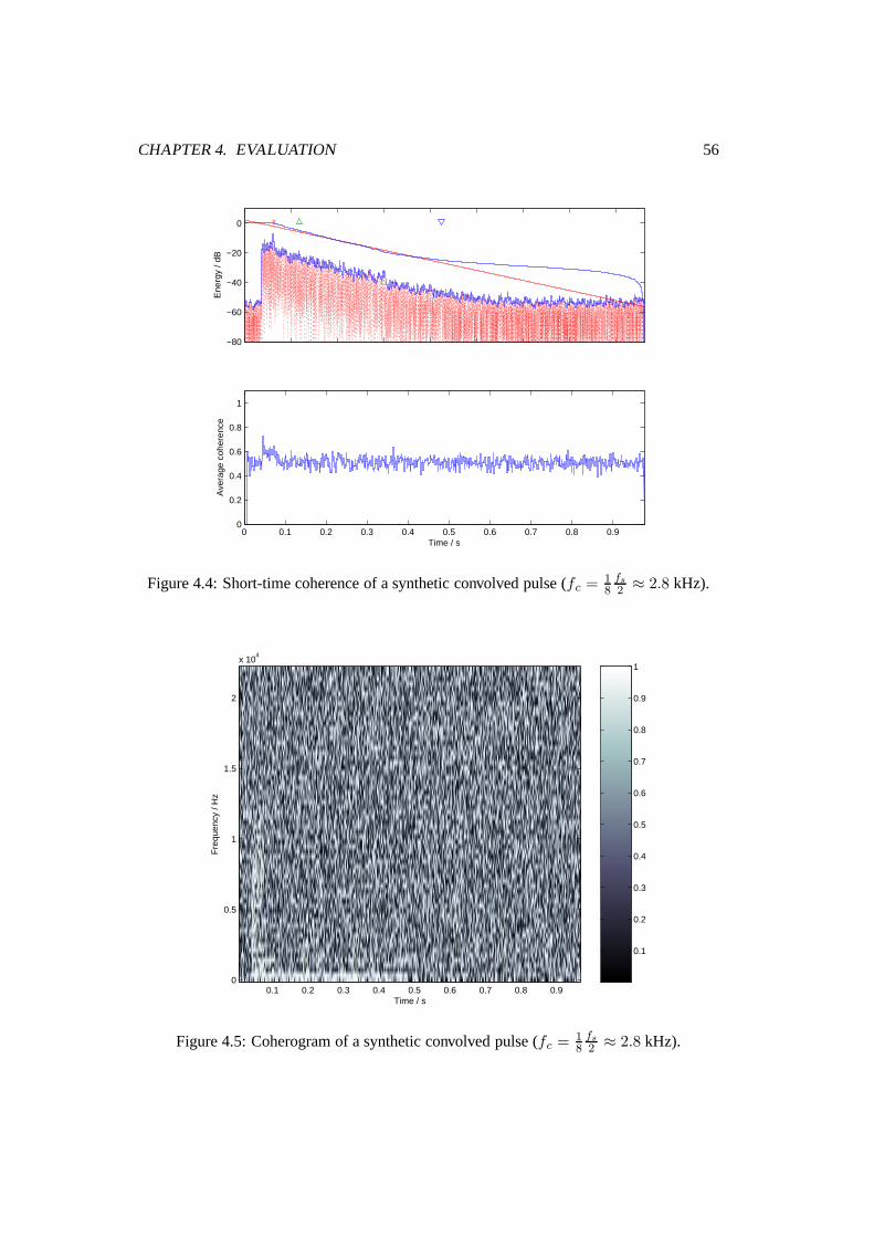
CHAPTER 4. EVALUATION 56
−80
−60
−40
−20
0E
nerg
y / d
B
0 0.1 0.2 0.3 0.4 0.5 0.6 0.7 0.8 0.90
0.2
0.4
0.6
0.8
1
Time / s
Ave
rage
coh
eren
ce
Figure 4.4: Short-time coherence of a synthetic convolved pulse (fc = 18
fs
2 ≈ 2.8 kHz).
Time / s
Fre
quen
cy /
Hz
0.1 0.2 0.3 0.4 0.5 0.6 0.7 0.8 0.90
0.5
1
1.5
2
x 104
0.1
0.2
0.3
0.4
0.5
0.6
0.7
0.8
0.9
1
Figure 4.5: Coherogram of a synthetic convolved pulse (fc = 18
fs
2 ≈ 2.8 kHz).
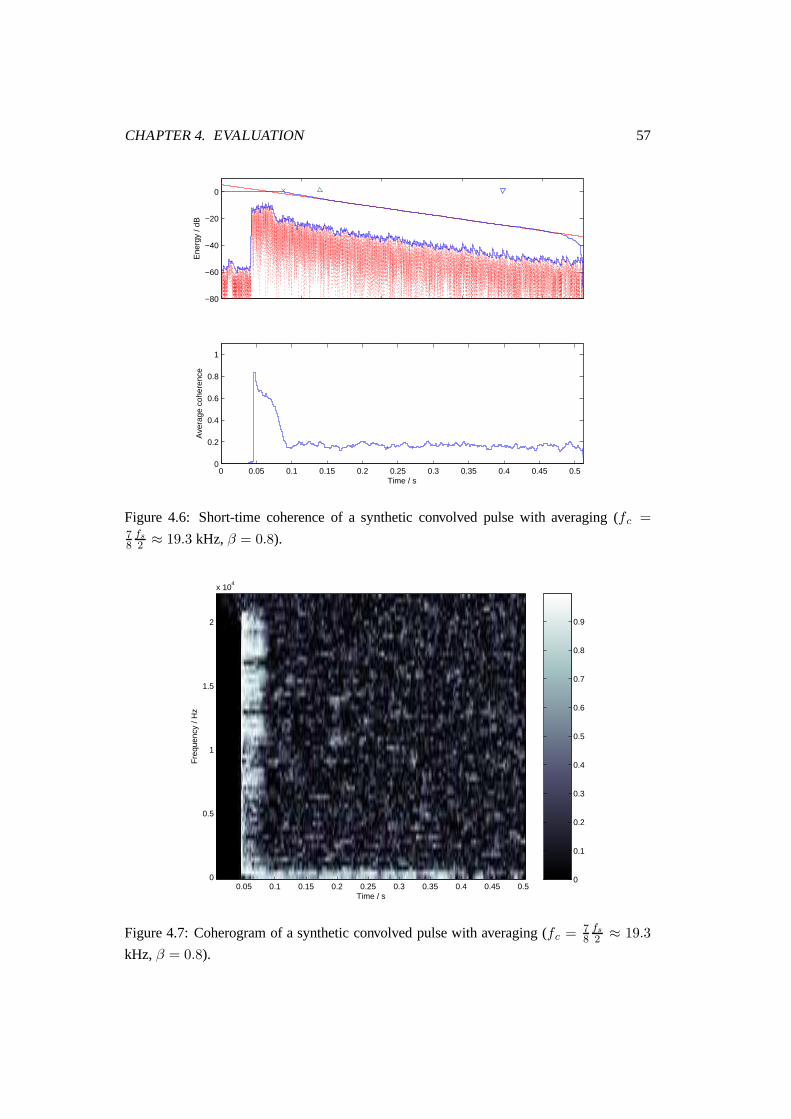
CHAPTER 4. EVALUATION 57
−80
−60
−40
−20
0E
nerg
y / d
B
0 0.05 0.1 0.15 0.2 0.25 0.3 0.35 0.4 0.45 0.50
0.2
0.4
0.6
0.8
1
Time / s
Ave
rage
coh
eren
ce
Figure 4.6: Short-time coherence of a synthetic convolved pulse with averaging (fc =78
fs
2 ≈ 19.3 kHz, β = 0.8).
Time / s
Fre
quen
cy /
Hz
0.05 0.1 0.15 0.2 0.25 0.3 0.35 0.4 0.45 0.50
0.5
1
1.5
2
x 104
0
0.1
0.2
0.3
0.4
0.5
0.6
0.7
0.8
0.9
Figure 4.7: Coherogram of a synthetic convolved pulse with averaging (fc = 78
fs
2 ≈ 19.3
kHz, β = 0.8).
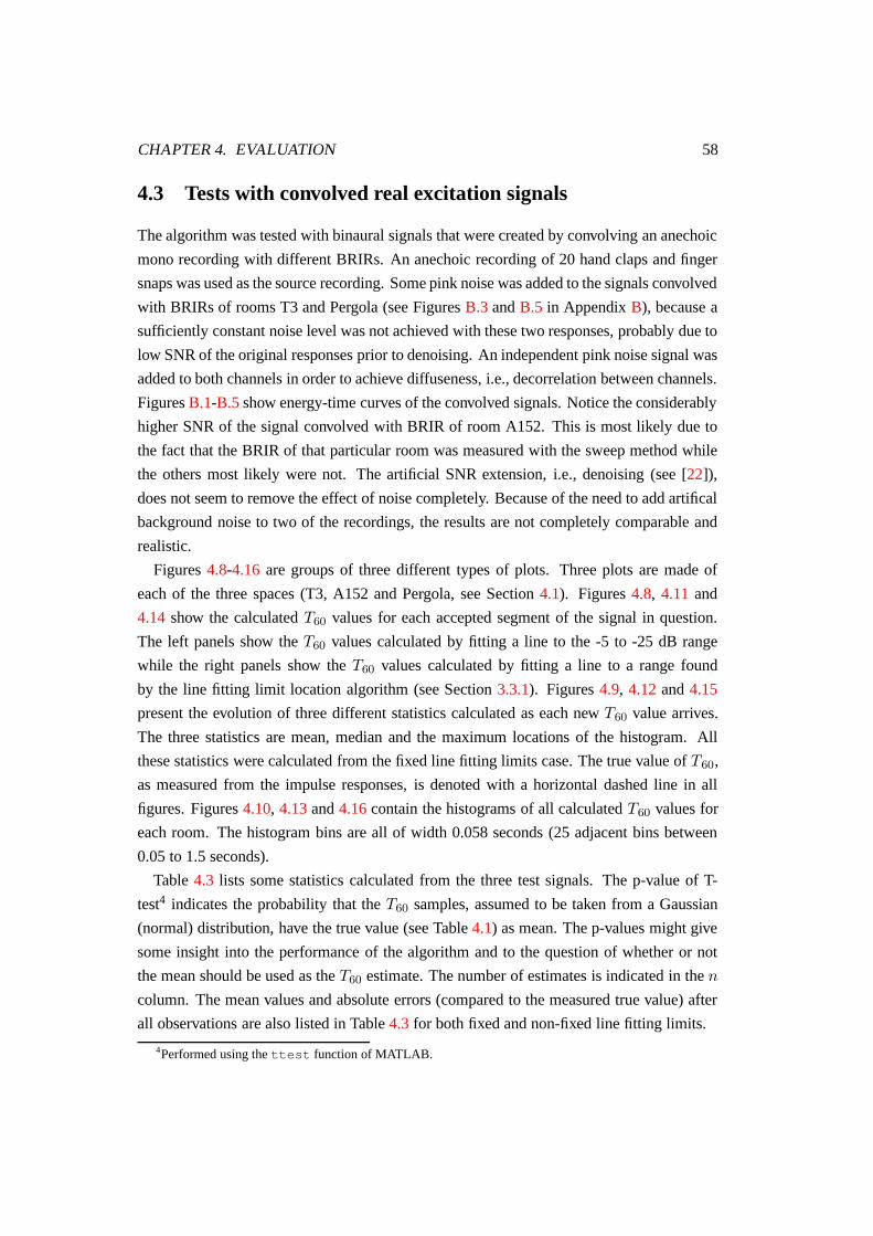
CHAPTER 4. EVALUATION 58
4.3 Tests with convolved real excitation signals
The algorithm was tested with binaural signals that were created by convolving an anechoic
mono recording with different BRIRs. An anechoic recording of 20 hand claps and finger
snaps was used as the source recording. Some pink noise was added to the signals convolved
with BRIRs of rooms T3 and Pergola (see Figures B.3 and B.5 in Appendix B), because a
sufficiently constant noise level was not achieved with these two responses, probably due to
low SNR of the original responses prior to denoising. An independent pink noise signal was
added to both channels in order to achieve diffuseness, i.e., decorrelation between channels.
Figures B.1-B.5 show energy-time curves of the convolved signals. Notice the considerably
higher SNR of the signal convolved with BRIR of room A152. This is most likely due to
the fact that the BRIR of that particular room was measured with the sweep method while
the others most likely were not. The artificial SNR extension, i.e., denoising (see [22]),
does not seem to remove the effect of noise completely. Because of the need to add artifical
background noise to two of the recordings, the results are not completely comparable and
realistic.
Figures 4.8-4.16 are groups of three different types of plots. Three plots are made of
each of the three spaces (T3, A152 and Pergola, see Section 4.1). Figures 4.8, 4.11 and
4.14 show the calculated T60 values for each accepted segment of the signal in question.
The left panels show the T60 values calculated by fitting a line to the -5 to -25 dB range
while the right panels show the T60 values calculated by fitting a line to a range found
by the line fitting limit location algorithm (see Section 3.3.1). Figures 4.9, 4.12 and 4.15
present the evolution of three different statistics calculated as each new T60 value arrives.
The three statistics are mean, median and the maximum locations of the histogram. All
these statistics were calculated from the fixed line fitting limits case. The true value of T60,
as measured from the impulse responses, is denoted with a horizontal dashed line in all
figures. Figures 4.10, 4.13 and 4.16 contain the histograms of all calculated T60 values for
each room. The histogram bins are all of width 0.058 seconds (25 adjacent bins between
0.05 to 1.5 seconds).
Table 4.3 lists some statistics calculated from the three test signals. The p-value of T-
test4 indicates the probability that the T60 samples, assumed to be taken from a Gaussian
(normal) distribution, have the true value (see Table 4.1) as mean. The p-values might give
some insight into the performance of the algorithm and to the question of whether or not
the mean should be used as the T60 estimate. The number of estimates is indicated in the n
column. The mean values and absolute errors (compared to the measured true value) after
all observations are also listed in Table 4.3 for both fixed and non-fixed line fitting limits.
4Performed using the ttest function of MATLAB.
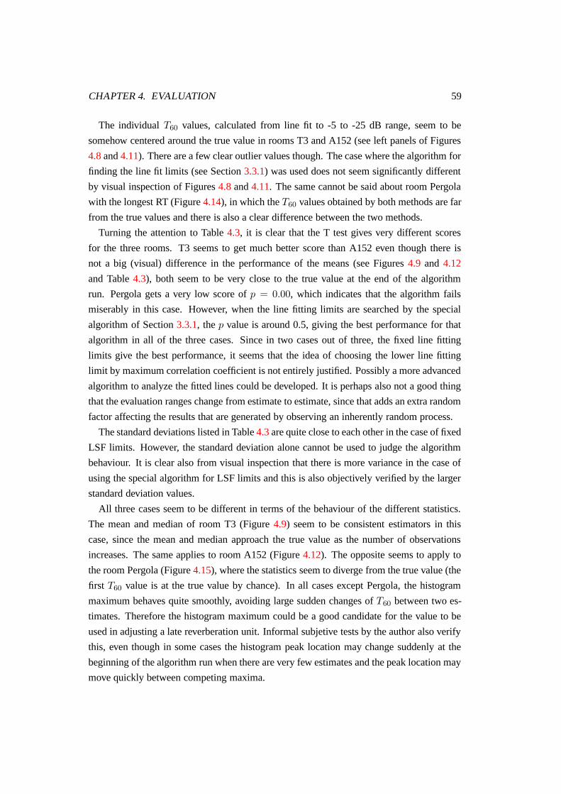
CHAPTER 4. EVALUATION 59
The individual T60 values, calculated from line fit to -5 to -25 dB range, seem to be
somehow centered around the true value in rooms T3 and A152 (see left panels of Figures
4.8 and 4.11). There are a few clear outlier values though. The case where the algorithm for
finding the line fit limits (see Section 3.3.1) was used does not seem significantly different
by visual inspection of Figures 4.8 and 4.11. The same cannot be said about room Pergola
with the longest RT (Figure 4.14), in which the T60 values obtained by both methods are far
from the true values and there is also a clear difference between the two methods.
Turning the attention to Table 4.3, it is clear that the T test gives very different scores
for the three rooms. T3 seems to get much better score than A152 even though there is
not a big (visual) difference in the performance of the means (see Figures 4.9 and 4.12
and Table 4.3), both seem to be very close to the true value at the end of the algorithm
run. Pergola gets a very low score of p = 0.00, which indicates that the algorithm fails
miserably in this case. However, when the line fitting limits are searched by the special
algorithm of Section 3.3.1, the p value is around 0.5, giving the best performance for that
algorithm in all of the three cases. Since in two cases out of three, the fixed line fitting
limits give the best performance, it seems that the idea of choosing the lower line fitting
limit by maximum correlation coefficient is not entirely justified. Possibly a more advanced
algorithm to analyze the fitted lines could be developed. It is perhaps also not a good thing
that the evaluation ranges change from estimate to estimate, since that adds an extra random
factor affecting the results that are generated by observing an inherently random process.
The standard deviations listed in Table 4.3 are quite close to each other in the case of fixed
LSF limits. However, the standard deviation alone cannot be used to judge the algorithm
behaviour. It is clear also from visual inspection that there is more variance in the case of
using the special algorithm for LSF limits and this is also objectively verified by the larger
standard deviation values.
All three cases seem to be different in terms of the behaviour of the different statistics.
The mean and median of room T3 (Figure 4.9) seem to be consistent estimators in this
case, since the mean and median approach the true value as the number of observations
increases. The same applies to room A152 (Figure 4.12). The opposite seems to apply to
the room Pergola (Figure 4.15), where the statistics seem to diverge from the true value (the
first T60 value is at the true value by chance). In all cases except Pergola, the histogram
maximum behaves quite smoothly, avoiding large sudden changes of T60 between two es-
timates. Therefore the histogram maximum could be a good candidate for the value to be
used in adjusting a late reverberation unit. Informal subjetive tests by the author also verify
this, even though in some cases the histogram peak location may change suddenly at the
beginning of the algorithm run when there are very few estimates and the peak location may
move quickly between competing maxima.
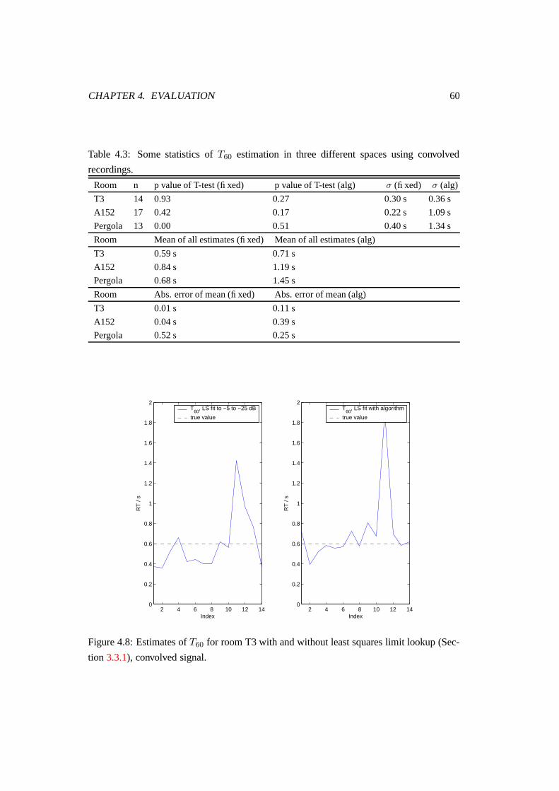
CHAPTER 4. EVALUATION 60
Table 4.3: Some statistics of T60 estimation in three different spaces using convolved
recordings.
Room n p value of T-test (fixed) p value of T-test (alg) σ (fixed) σ (alg)
T3 14 0.93 0.27 0.30 s 0.36 s
A152 17 0.42 0.17 0.22 s 1.09 s
Pergola 13 0.00 0.51 0.40 s 1.34 s
Room Mean of all estimates (fixed) Mean of all estimates (alg)
T3 0.59 s 0.71 s
A152 0.84 s 1.19 s
Pergola 0.68 s 1.45 s
Room Abs. error of mean (fixed) Abs. error of mean (alg)
T3 0.01 s 0.11 s
A152 0.04 s 0.39 s
Pergola 0.52 s 0.25 s
2 4 6 8 10 12 140
0.2
0.4
0.6
0.8
1
1.2
1.4
1.6
1.8
2
RT
/ s
Index
T60
, LS fit to −5 to −25 dB
true value
2 4 6 8 10 12 140
0.2
0.4
0.6
0.8
1
1.2
1.4
1.6
1.8
2
RT
/ s
Index
T60
, LS fit with algorithm
true value
Figure 4.8: Estimates of T60 for room T3 with and without least squares limit lookup (Sec-
tion 3.3.1), convolved signal.
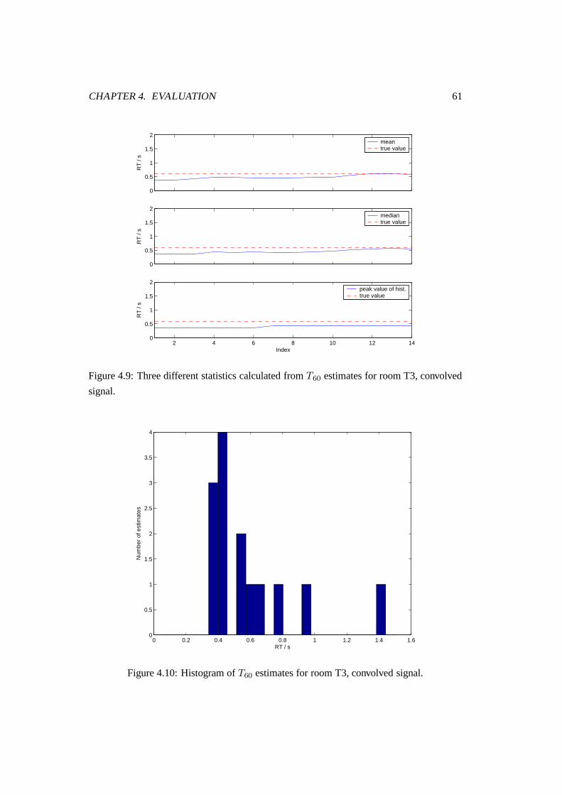
CHAPTER 4. EVALUATION 61
0
0.5
1
1.5
2R
T /
smeantrue value
0
0.5
1
1.5
2
RT
/ s
mediantrue value
2 4 6 8 10 12 140
0.5
1
1.5
2
RT
/ s
Index
peak value of hist.true value
Figure 4.9: Three different statistics calculated from T60 estimates for room T3, convolved
signal.
0 0.2 0.4 0.6 0.8 1 1.2 1.4 1.60
0.5
1
1.5
2
2.5
3
3.5
4
Num
ber
of e
stim
ates
RT / s
Figure 4.10: Histogram of T60 estimates for room T3, convolved signal.
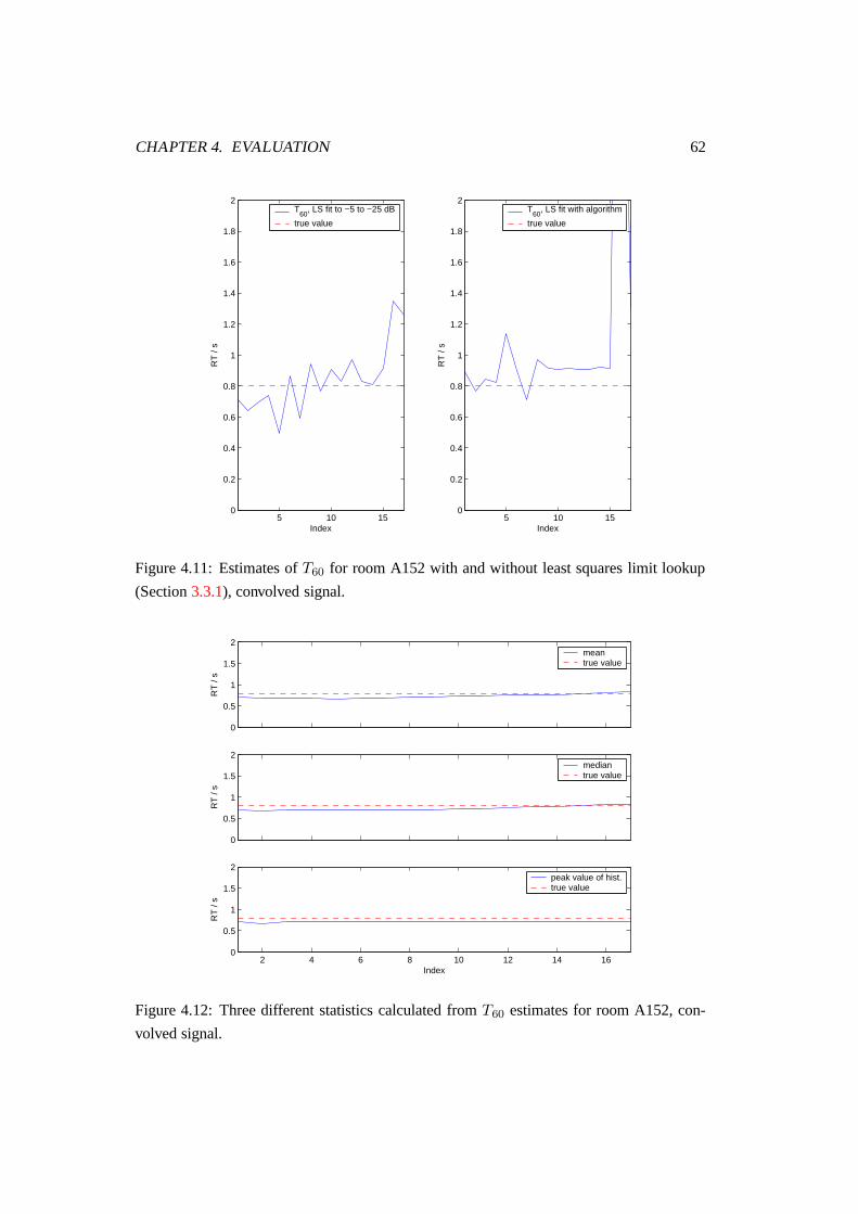
CHAPTER 4. EVALUATION 62
5 10 150
0.2
0.4
0.6
0.8
1
1.2
1.4
1.6
1.8
2
RT
/ s
Index
T60
, LS fit to −5 to −25 dB
true value
5 10 150
0.2
0.4
0.6
0.8
1
1.2
1.4
1.6
1.8
2
RT
/ s
Index
T60
, LS fit with algorithm
true value
Figure 4.11: Estimates of T60 for room A152 with and without least squares limit lookup
(Section 3.3.1), convolved signal.
0
0.5
1
1.5
2
RT
/ s
meantrue value
0
0.5
1
1.5
2
RT
/ s
mediantrue value
2 4 6 8 10 12 14 160
0.5
1
1.5
2
RT
/ s
Index
peak value of hist.true value
Figure 4.12: Three different statistics calculated from T60 estimates for room A152, con-
volved signal.
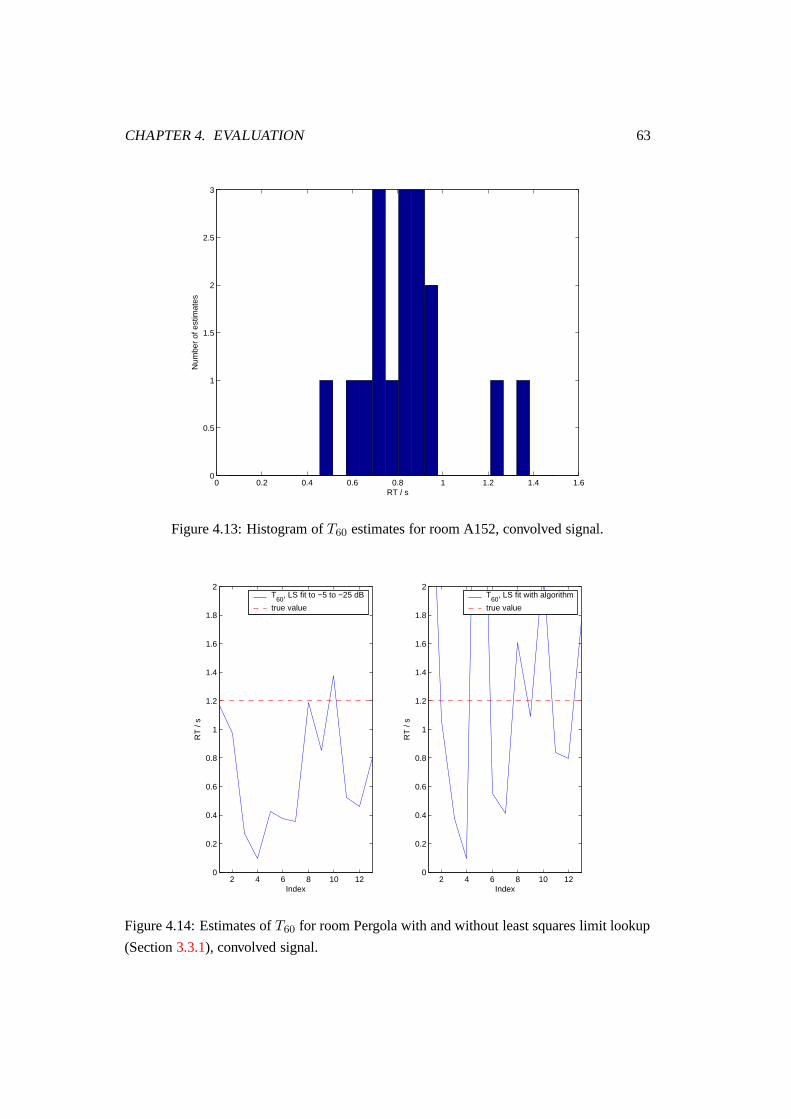
CHAPTER 4. EVALUATION 63
0 0.2 0.4 0.6 0.8 1 1.2 1.4 1.60
0.5
1
1.5
2
2.5
3N
umbe
r of
est
imat
es
RT / s
Figure 4.13: Histogram of T60 estimates for room A152, convolved signal.
2 4 6 8 10 120
0.2
0.4
0.6
0.8
1
1.2
1.4
1.6
1.8
2
RT
/ s
Index
T60
, LS fit to −5 to −25 dB
true value
2 4 6 8 10 120
0.2
0.4
0.6
0.8
1
1.2
1.4
1.6
1.8
2
RT
/ s
Index
T60
, LS fit with algorithm
true value
Figure 4.14: Estimates of T60 for room Pergola with and without least squares limit lookup
(Section 3.3.1), convolved signal.
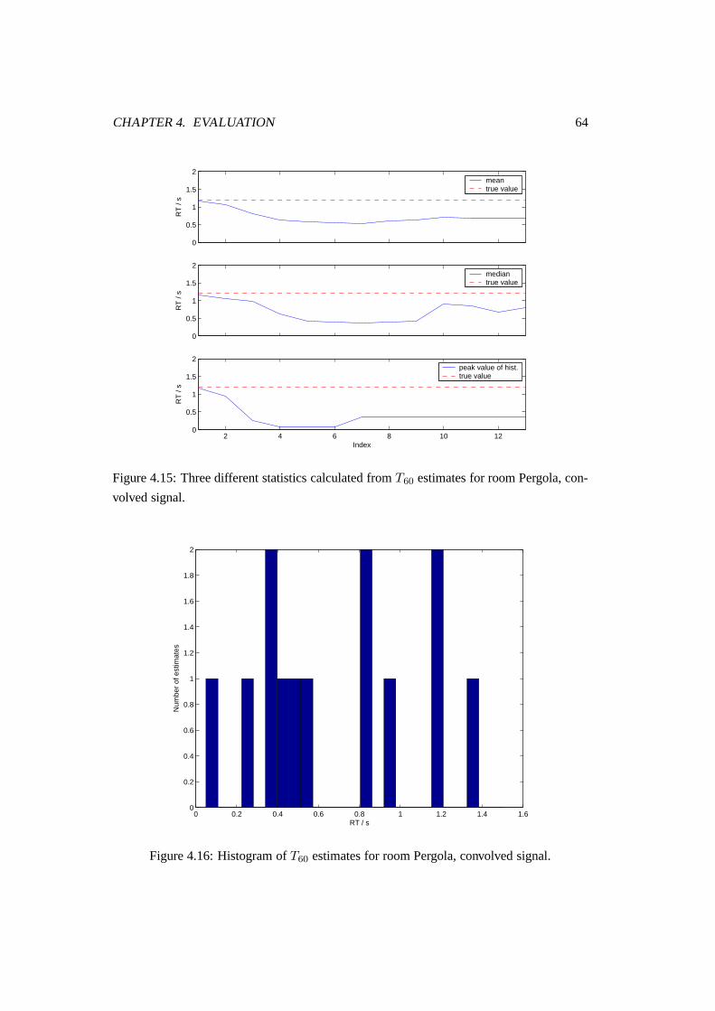
CHAPTER 4. EVALUATION 64
0
0.5
1
1.5
2R
T /
smeantrue value
0
0.5
1
1.5
2
RT
/ s
mediantrue value
2 4 6 8 10 120
0.5
1
1.5
2
RT
/ s
Index
peak value of hist.true value
Figure 4.15: Three different statistics calculated from T60 estimates for room Pergola, con-
volved signal.
0 0.2 0.4 0.6 0.8 1 1.2 1.4 1.60
0.2
0.4
0.6
0.8
1
1.2
1.4
1.6
1.8
2
Num
ber
of e
stim
ates
RT / s
Figure 4.16: Histogram of T60 estimates for room Pergola, convolved signal.
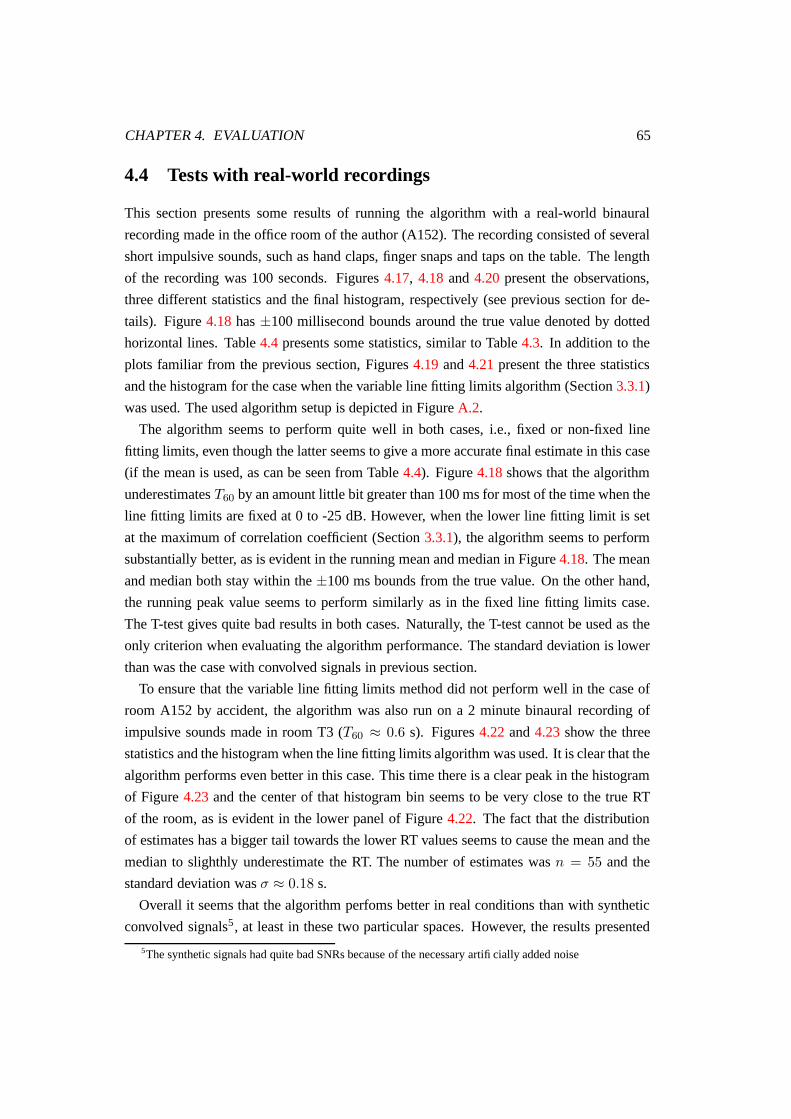
CHAPTER 4. EVALUATION 65
4.4 Tests with real-world recordings
This section presents some results of running the algorithm with a real-world binaural
recording made in the office room of the author (A152). The recording consisted of several
short impulsive sounds, such as hand claps, finger snaps and taps on the table. The length
of the recording was 100 seconds. Figures 4.17, 4.18 and 4.20 present the observations,
three different statistics and the final histogram, respectively (see previous section for de-
tails). Figure 4.18 has ±100 millisecond bounds around the true value denoted by dotted
horizontal lines. Table 4.4 presents some statistics, similar to Table 4.3. In addition to the
plots familiar from the previous section, Figures 4.19 and 4.21 present the three statistics
and the histogram for the case when the variable line fitting limits algorithm (Section 3.3.1)
was used. The used algorithm setup is depicted in Figure A.2.
The algorithm seems to perform quite well in both cases, i.e., fixed or non-fixed line
fitting limits, even though the latter seems to give a more accurate final estimate in this case
(if the mean is used, as can be seen from Table 4.4). Figure 4.18 shows that the algorithm
underestimates T60 by an amount little bit greater than 100 ms for most of the time when the
line fitting limits are fixed at 0 to -25 dB. However, when the lower line fitting limit is set
at the maximum of correlation coefficient (Section 3.3.1), the algorithm seems to perform
substantially better, as is evident in the running mean and median in Figure 4.18. The mean
and median both stay within the ±100 ms bounds from the true value. On the other hand,
the running peak value seems to perform similarly as in the fixed line fitting limits case.
The T-test gives quite bad results in both cases. Naturally, the T-test cannot be used as the
only criterion when evaluating the algorithm performance. The standard deviation is lower
than was the case with convolved signals in previous section.
To ensure that the variable line fitting limits method did not perform well in the case of
room A152 by accident, the algorithm was also run on a 2 minute binaural recording of
impulsive sounds made in room T3 (T60 ≈ 0.6 s). Figures 4.22 and 4.23 show the three
statistics and the histogram when the line fitting limits algorithm was used. It is clear that the
algorithm performs even better in this case. This time there is a clear peak in the histogram
of Figure 4.23 and the center of that histogram bin seems to be very close to the true RT
of the room, as is evident in the lower panel of Figure 4.22. The fact that the distribution
of estimates has a bigger tail towards the lower RT values seems to cause the mean and the
median to slighthly underestimate the RT. The number of estimates was n = 55 and the
standard deviation was σ ≈ 0.18 s.
Overall it seems that the algorithm perfoms better in real conditions than with synthetic
convolved signals5 , at least in these two particular spaces. However, the results presented
5The synthetic signals had quite bad SNRs because of the necessary artificially added noise
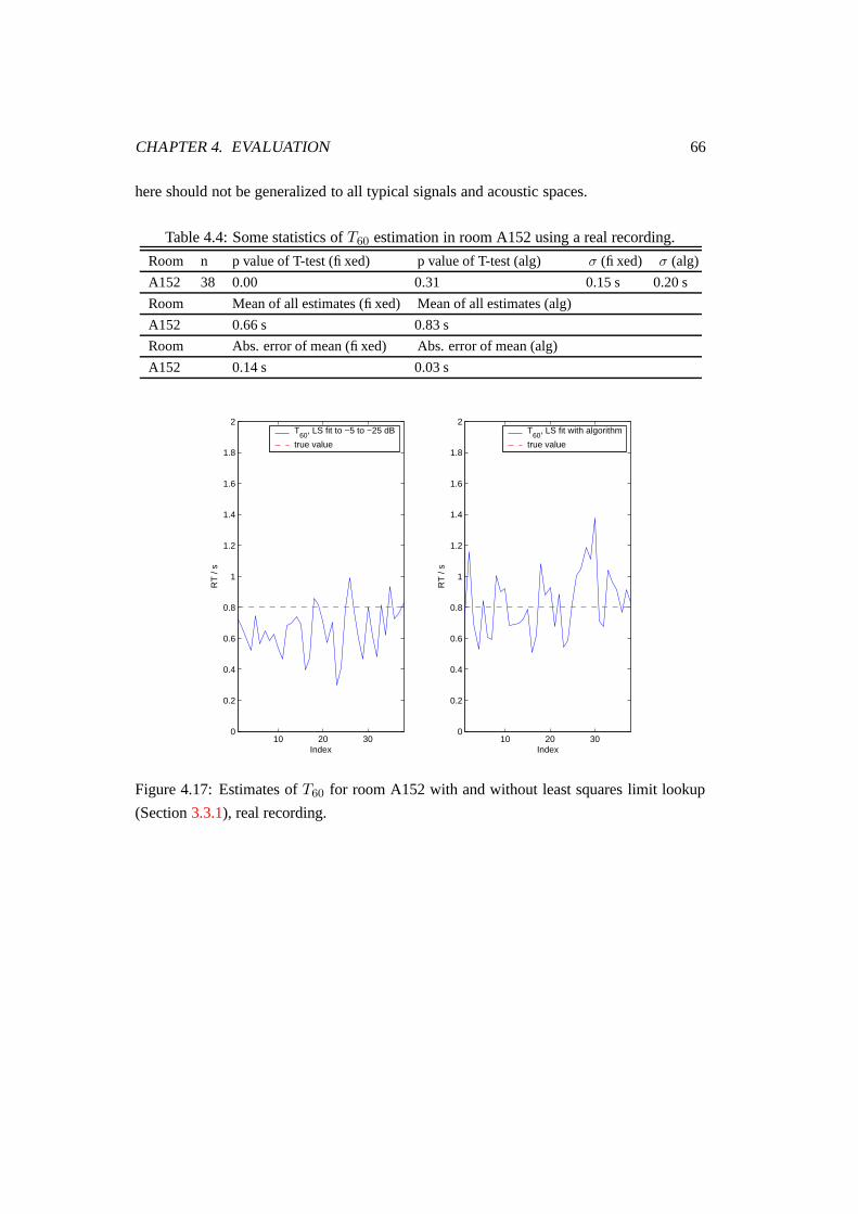
CHAPTER 4. EVALUATION 66
here should not be generalized to all typical signals and acoustic spaces.
Table 4.4: Some statistics of T60 estimation in room A152 using a real recording.
Room n p value of T-test (fixed) p value of T-test (alg) σ (fixed) σ (alg)
A152 38 0.00 0.31 0.15 s 0.20 s
Room Mean of all estimates (fixed) Mean of all estimates (alg)
A152 0.66 s 0.83 s
Room Abs. error of mean (fixed) Abs. error of mean (alg)
A152 0.14 s 0.03 s
10 20 300
0.2
0.4
0.6
0.8
1
1.2
1.4
1.6
1.8
2
RT
/ s
Index
T60
, LS fit to −5 to −25 dB
true value
10 20 300
0.2
0.4
0.6
0.8
1
1.2
1.4
1.6
1.8
2
RT
/ s
Index
T60
, LS fit with algorithm
true value
Figure 4.17: Estimates of T60 for room A152 with and without least squares limit lookup
(Section 3.3.1), real recording.
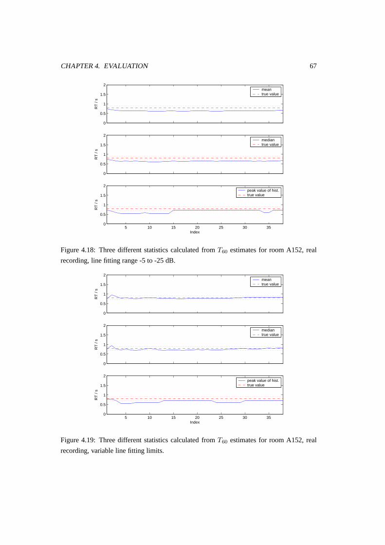
CHAPTER 4. EVALUATION 67
0
0.5
1
1.5
2
RT
/ s
meantrue value
0
0.5
1
1.5
2
RT
/ s
mediantrue value
5 10 15 20 25 30 350
0.5
1
1.5
2
RT
/ s
Index
peak value of hist.true value
Figure 4.18: Three different statistics calculated from T60 estimates for room A152, real
recording, line fitting range -5 to -25 dB.
0
0.5
1
1.5
2
RT
/ s
meantrue value
0
0.5
1
1.5
2
RT
/ s
mediantrue value
5 10 15 20 25 30 350
0.5
1
1.5
2
RT
/ s
Index
peak value of hist.true value
Figure 4.19: Three different statistics calculated from T60 estimates for room A152, real
recording, variable line fitting limits.
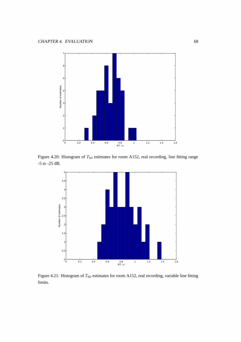
CHAPTER 4. EVALUATION 68
0 0.2 0.4 0.6 0.8 1 1.2 1.4 1.60
1
2
3
4
5
6
7
Num
ber
of e
stim
ates
RT / s
Figure 4.20: Histogram of T60 estimates for room A152, real recording, line fitting range
-5 to -25 dB.
0 0.2 0.4 0.6 0.8 1 1.2 1.4 1.60
0.5
1
1.5
2
2.5
3
3.5
4
4.5
5
Num
ber
of e
stim
ates
RT / s
Figure 4.21: Histogram of T60 estimates for room A152, real recording, variable line fitting
limits.
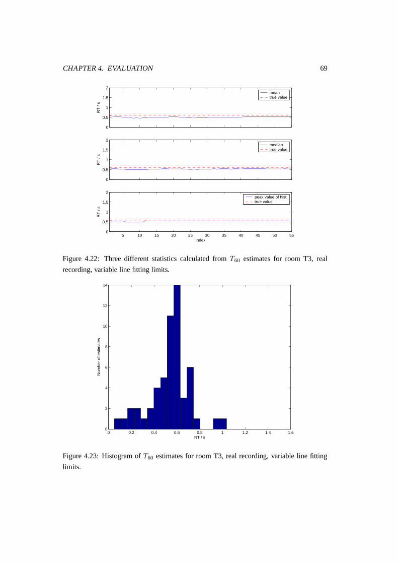
CHAPTER 4. EVALUATION 69
0
0.5
1
1.5
2
RT
/ s
meantrue value
0
0.5
1
1.5
2
RT
/ s
mediantrue value
5 10 15 20 25 30 35 40 45 50 550
0.5
1
1.5
2
RT
/ s
Index
peak value of hist.true value
Figure 4.22: Three different statistics calculated from T60 estimates for room T3, real
recording, variable line fitting limits.
0 0.2 0.4 0.6 0.8 1 1.2 1.4 1.60
2
4
6
8
10
12
14
Num
ber
of e
stim
ates
RT / s
Figure 4.23: Histogram of T60 estimates for room T3, real recording, variable line fitting
limits.
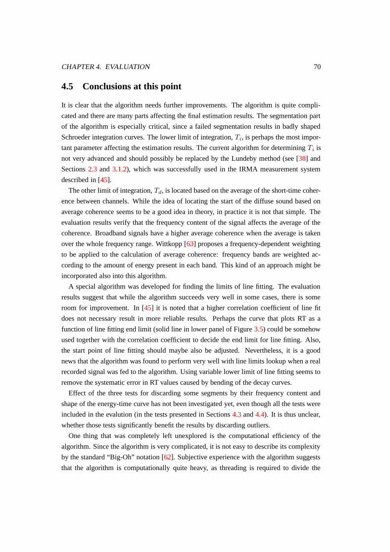
CHAPTER 4. EVALUATION 70
4.5 Conclusions at this point
It is clear that the algorithm needs further improvements. The algorithm is quite compli-
cated and there are many parts affecting the final estimation results. The segmentation part
of the algorithm is especially critical, since a failed segmentation results in badly shaped
Schroeder integration curves. The lower limit of integration, Ti, is perhaps the most impor-
tant parameter affecting the estimation results. The current algorithm for determining Ti is
not very advanced and should possibly be replaced by the Lundeby method (see [38] and
Sections 2.3 and 3.1.2), which was successfully used in the IRMA measurement system
described in [45].
The other limit of integration, Td, is located based on the average of the short-time coher-
ence between channels. While the idea of locating the start of the diffuse sound based on
average coherence seems to be a good idea in theory, in practice it is not that simple. The
evaluation results verify that the frequency content of the signal affects the average of the
coherence. Broadband signals have a higher average coherence when the average is taken
over the whole frequency range. Wittkopp [63] proposes a frequency-dependent weighting
to be applied to the calculation of average coherence: frequency bands are weighted ac-
cording to the amount of energy present in each band. This kind of an approach might be
incorporated also into this algorithm.
A special algorithm was developed for finding the limits of line fitting. The evaluation
results suggest that while the algorithm succeeds very well in some cases, there is some
room for improvement. In [45] it is noted that a higher correlation coefficient of line fit
does not necessary result in more reliable results. Perhaps the curve that plots RT as a
function of line fitting end limit (solid line in lower panel of Figure 3.5) could be somehow
used together with the correlation coefficient to decide the end limit for line fitting. Also,
the start point of line fitting should maybe also be adjusted. Nevertheless, it is a good
news that the algorithm was found to perform very well with line limits lookup when a real
recorded signal was fed to the algorithm. Using variable lower limit of line fitting seems to
remove the systematic error in RT values caused by bending of the decay curves.
Effect of the three tests for discarding some segments by their frequency content and
shape of the energy-time curve has not been investigated yet, even though all the tests were
included in the evalution (in the tests presented in Sections 4.3 and 4.4). It is thus unclear,
whether those tests significantly benefit the results by discarding outliers.
One thing that was completely left unexplored is the computational efficiency of the
algorithm. Since the algorithm is very complicated, it is not easy to describe its complexity
by the standard “Big-Oh” notation [62]. Subjective experience with the algorithm suggests
that the algorithm is computationally quite heavy, as threading is required to divide the
CHAPTER 4. EVALUATION 71
computational burden over a longer time6. A few buffer underflows also occurred during
the evaluation runs, i.e., the real-time algorithm did not have time to process all incoming
data. Because of this, two algorithm runs on a same audio file might give slightly different
results.
6The algorithm was ran real-time on a 1.6 GHz Linux PC.
Chapter 5
Conclusions
The main goal of this work was to develop a method for estimating the reverberation time
from a binaural signal when the excitation signal cannot be controlled, i.e., the input signal
to the algorithm is arbitrary. It was hypothesized that the binaural nature of the signals could
be exploited to distinguish the diffuse decay from the direct sound and early reflections.
This would make it possible to accurately locate the starting point for reverberation time
analysis, which was decided to be based on the well-known Schroeder method. The whole
approach for reverberation time estimation was based on the idea of locating interesting
sound events from the input signal and then subjecting the obtained signal segments to
subsequent analysis. This approach is related to the auditory decomposition (see Section
1.1.3), part of which is the detection and localization of interesting sound events in the
environment around a listener, solely based on the binaural signals.
It is clear that the approach chosen in this work has some inherent problems. The most
important of them is that the algorithm requires transient excitation sounds for RT estima-
tion. This leaves many usable longer sounds with a sudden offset, which is followed by
a reverberant tail, out of the analysis. Because of this, the algorithm cannot determine RT
from speech, which is a very important and common signal class in everyday environments.
A natural future improvement to the algorithm would be rewriting the coarse segmentation
part. The most similar RT estimation algorithm reported in literature [61] performs the
analysis on signal segments that have decreasing energy. The criterion of decreasing energy
could also be included in the coarse segmentation algorithm of this work, so that instead
of looking for transient sounds, the algorithm would find the parts of the signal that have a
sound event onset with large enough SNR, which is later followed by a decrease in energy
with a steep enough slope. Only the part of the segment with decreasing energy would be
included in subsequent analysis. This way the algorithm would get a lot more estimates in
a normal environment, which normally does not have very many transient sounds.
72
CHAPTER 5. CONCLUSIONS 73
Nevertheless, the algorithm performs quite fine in a real environment, as was found out
in Chapter 4. The method for finding the line fitting limits (Section 3.3.1) works quite well
for real signals and significantly improves the accuracy of the RT estimations. It would
be interesting to compare the algorithm performance to the RT discrimination abilities of
humans. Naturally, humans can rarely give an absolute RT value for a room, but they can
discriminate changes in the environment. According to [43], the difference limen for rever-
beration time is on the order of 40 ms in rooms with mid-frequency T60 < 600 ms. Another
study reported the mean upper and lower just noticeable differences for reverberated speech
to be in the range of 3.3 − 9.6 % of the corresponding RT [25]. Since one of the main ap-
plications of this algorithm was to use the estimated RT to adjust a late reverberation unit
of an augmented reality application (see Section 1.1), it would be advantageous to match
the RT as closely to the surrounding space as possible. The algorithm estimated the RT to
an accuracy ranging from 10 to 500 ms, depending on the room and the statistics used. The
algorithm therefore matches the difference limen of humans at its best. But it is unclear
how big changes between the true RT of a room and the RT of the artificially added sound
sources is allowed for the listener to perceive the augmented sources as not belonging to the
environment around the listener.
Automatic estimation of reverberation time is a relatively unexplored topic in the area
of audio signal processing. There are not very many different algorithms mentioned in the
literature at the moment. The work described in this thesis provides some new contributions
to the field of automatic RT estimation. While the algorithm is quite choosy about the
sounds that it accepts, the quality of the estimates is relatively high. A downside of the
algorithm is its complexity, in both computational and algorithmic sense. There are more
than 10 adjustable parameters, which is quite a lot. However, once a good combination of
parameter values is found, there is no need for re-adjusting them.
Bibliography
[1] Alexis Baskind and Olivier Warusfel. Methods for Blind Computational Estimation
of Perceptual Attributes of Room Acoustics. In Proceedings of the AES 22nd Inter-
national Conference on Virtual, Synthetic and Entertainment Audio (AES22), Espoo,
Finland, June 2002.
[2] Julius S. Bendat and Allan G. Piersol. Engineering Applications of Correlation and
Spectral Analysis. John Wiley & Sons Ltd, 1980.
[3] Leo Beranek. Concert and Opera Halls - How They Sound. The Acoustical Society
of America, New York, 1984.
[4] Alan C. Bovik, Thomas S. Huang, and Jr. David C. Munson. A Generalization of Me-
dian Filtering Using Linear Combinations of Order Statistics. IEEE Transactions on
Acoustics, Speech, and Signal Processing, ASSP-31(6):1342–1350, December 1972.
[5] G. Clifford Carter, Charles H. Knapp, and Albert H. Nuttall. Estimation of the
Magnitude-Squared Coherence Function Via Overlapped Fast Fourier Transform Pro-
cessing. IEEE Transactions on Audio and Electroacoustics, AU-21(4):337–344, 1972.
[6] Michael A. Casey. MPEG-7 Sound-Recognition Tools. IEEE Transactions on Circuits
and Systems for Video Technology, 11(6):737–747, 2001.
[7] W. T. Chu. Comparison of Reverberation Measurements Using Schroeder’s Impulse
Method and Decay-Curve Averaging Method. Journal of The Acoustical Society of
America, 63(5):1444–1450, 1978.
[8] Laurent Couvreur and Christophe Couvreur. Robust Automatic Speech Recognition
in Reverberant Environments by Model Selection. In Proceedings of the International
Workshop on Hands-Free Speech Communication (HSC-2001), pages 147–150, Ky-
oto, Japan, April 2001.
74
BIBLIOGRAPHY 75
[9] Laurent Couvreur, Christophe Ris, and Christophe Couvreur. Model-based Blind Es-
timation of Reverberation Time: Application to Robust ASR in Reverberant Environ-
ments. In Proceedings of the European Conference on Speech Communication and
Technology (EUROSPEECH-2001), volume 1, pages 2631–2634, Aalborg, Denmark,
September 2001.
[10] Trevor J. Cox and Francis F. Li nand Paul Darlington. Extracting Room Reverberation
Time from Speech Using Artificial Neural Networks. Journal of The Audio Engineer-
ing Society, 49(4):219–230, April 2001.
[11] Manuel Davy and Simon Godsill. Detection of Abrupt Spectral Changes Using Sup-
port Vector Machines. In Proceedings of the IEEE International Conference on Acous-
tics, Speech, and Signal Processing (ICASSP 2002), Orlando, Florida, USA, May
2002. http://www.irccyn.ec-nantes.fr/˜davy/papers/davy-icassp2002.pdf.
[12] Frédéric Desobry and Manuel Davy. Support Vector-Based Online Detection of
Abrupt Changes. In Proceedings of the IEEE International Conference on Acous-
tics, Speech, and Signal Processing (ICASSP2003), Hong-Kong, China, April 2003.
http://www.irccyn.ec-nantes.fr/˜davy/papers/desobry-icassp-03.pdf.
[13] Sasha Devore and Barbara Shinn-Cunningham. Perceptual Consequences of Includ-
ing Reverberation in Spatial Auditory Displays. In Proceedings of the International
Conference on Auditory Display (ICAD-03), Boston, MA, USA, July 2003.
[14] Alain Dufaux, Laurent Besacier, Michael Ansorge, and Fausto Pellandini. Automatic
Sound Detection and Recognition for Noisy Environment. In Proceedings of the Euro-
pean Signal Processing Conference (EUSIPCO 2000), Tampere, Finland, September
2000.
[15] Antti Eronen, Juha Tuomi, Anssi Klapuri, Seppo Fagerlund, Timo Sorsa, Gaëtan
Lorho, and Jyri Huopaniemi. Audio-based Context Awareness - Acoustic Modeling
and Perceptual Evaluation. In Proceedings of the IEEE International Conference on
Acoustics, Speech, and Signal Processing (ICASSP2003), Hong-Kong, China, April
2003. http://www.cs.tut.fi/sgn/arg/music/eronen_icassp03.pdf.
[16] Laurent Faiget, Claude Legros, and Robert Ruiz. Optimization of the Impulse Re-
sponse Length: Application to Noisy and Highly Reverberant Rooms. Journal of The
Audio Engineering Society, 46(9):741–750, September 1998.
[17] Martin Hansen. A Method for Calculating Reverberation Time from Musical Signals.
Technical Report 60, The Acoustics Laboratory, Technical University of Denmark,
Building 352, DK-2800 Lynbgy, 1995.
BIBLIOGRAPHY 76
[18] Monson H. Hayes. Statistical Digital Signal Processing and Modeling. John Wiley &
Sons Ltd, 1996.
[19] Aki Härmä, Julia Jakka, Miikka Tikander, Matti Karjalainen, Tapio Lokki, Jarmo
Hiipakka, and Gaëtan Lorho. Augmented Reality Audio for Mobile and Wearable
Appliances. Journal of The Audio Engineering Society, 52(6):618–639, June 2004.
[20] Aki Härmä, Julia Jakka, Miikka Tikander, Matti Karjalainen, Tapio Lokki, Heli Niro-
nen, and Sampo Vesa. Techniques and Applications of Wearable Augmented Reality
Audio. In Proceedings of the AES 114th International Convention, Amsterdam, the
Netherlands, March 2003.
[21] Tommi Ilmonen. Mustajuuri - An Application and Toolkit for Interactive Audio Pro-
cessing. In Proceedings of the The Seventh International Conference on Auditory
Display (ICAD 2001), Espoo, Finland, July/August 2001.
[22] Jean-Marc Jot, Laurent Cerveau, and Olivier Warusfel. Analysis and Synthesis of
Room Reverberation Based on a Statistical Time-Frequency Model. In Proceedings
of the AES 103rd International Convention, New York, USA, 1997. Preprint 4629.
[23] Matti Karjalainen. Kommunikaatioakustiikka. Technical Report 51, Teknillinen kor-
keakoulu, Sähkö- ja tietoliikennetekniikan osasto, Akustiikan ja äänenkäsittelyteknii-
kan laboratorio, TKK, Otaniemi, 1999.
[24] Matti Karjalainen, Poju Antsalo, Aki Mäkivirta, Timo Peltonen, and Vesa Välimäki.
Estimation of Modal Decay Parameters from Noisy Response Measurements. Journal
of The Audio Engineering Society, 50(11):867–878, November 2002.
[25] Matti Karjalainen and Hanna Järveläinen. More About This Reverberation Science:
Perceptually Good Late Reverberation. In Proceedings of the AES 111th International
Convention, New York, USA, September 2001. Convention Paper 5415.
[26] Erwin Kreyszig. Advanced Engineering Mathematics. John Wiley & Sons Ltd, 7th
edition, 1993.
[27] Pauli Kuosmanen and Jaakko Astola. Fundamentals of Nonlinear Digital Filtering.
CRC Press Inc., 1998.
[28] Tapio Lahti. Akustinen mittaustekniikka. Technical Report 38, Teknillinen korkea-
koulu, sähkötekniikan osasto, akustiikan ja äänenkäsittelytekniikan laboratorio, TKK,
Otaniemi, 1995. Toinen korjattu painos 1997.
BIBLIOGRAPHY 77
[29] Hélène Laurent and Christian Doncarli. Abrupt Changes Detection in the Time-
Frequency Plane. In Proceedings of the IEEE-SP International Symposium on Time-
Scale Analysis, pages 285–288, Paris, France, 1996.
[30] Hélène Laurent and Christian Doncarli. Stationarity Index for Abrupt Changes De-
tection in the Time-Frequency Plane. IEEE Signal Processing Letters, 5(2):43–45,
1998.
[31] Hélène Laurent, Eric Hitti, and Marie-Francoise Lucas. Abrupt Changes Detection in
the Time-Scale and in the Time-Frequency Planes: a Comparative Study. In Proceed-
ings of the IEEE-SP International Symposium on Time-Scale Analysis, pages 501–504,
Pittsburgh, Philadelphia, USA, October 1998.
[32] Katia Lebart, Jean-Marc Boucher, and Philippe Denbigh. A New Method Based on
Spectral Subtraction for Speech Dereverberation. Acustica/Acta Acustica, 87(3):359–
366, 2001.
[33] Sébastien Lefèvre, Benjamin Maillard, and Nicole Vincent. A Two Level Classifier
Process for Audio Segmentation. In Proceedings of the IAPR International Confer-
ence on Pattern Recognition, pages 891–894, Quebec City, Canada, August 2002.
[34] Stan Z. Li. Content-Based Audio Classification and Retrieval Using the Nearest Fea-
ture Line Method. IEEE Signal Processing Letters, 8(5):619–625, September 2000.
[35] Chen Liu, Bruce C. Wheeler, William D. O’Brien Jr., Robert C. Bilger, Charissa R.
Lansing, and Albert S. Feng. Localization of Multiple Sound Sources with Two Mi-
crophones. Journal of The Acoustical Society of America, 108(4):1888–1905, October
2003.
[36] Tapio Lokki, Heli Nironen, Sampo Vesa, Lauri Savioja, Aki Härmä, and Matti Kar-
jalainen. Application Scenarios of Wearable and Mobile Augmented Reality Audio.
In Proceedings of the AES 116th International Convention, Berlin, Germany, May
2004.
[37] Lie Lu, Hao Jiang, and Hong Zhang. A robust audio classification and segmentation
method. In Proceedings of the 9th ACM International Conference on Multimedia,
pages 203–211. ACM Press, 2001.
[38] Anders Lundeby, Tor Erik Vigran, Heinrich Bietz, and Michael Vorländer. Uncertain-
ties of Measurements in Room Acoustics. Acustica, 81:344–355, 1995. Dedicated to
Prof. Dr. Heinrich Kuttruff on the occasion of his 65th birthday.
BIBLIOGRAPHY 78
[39] Janet S. Milton and Jesse C. Arnold. Introduction to Probability and Statistics.
McGraw-Hill, 2nd edition, 1990.
[40] Sanjit K. Mitra. Digital Signal Processing - A Computer-Based Approach. McGraw-
Hill, 2nd edition, 2001.
[41] Dennis R. Morgan. A Parametric Error Analysis of the Backward Integration Method
for Reverberation Time Estimation. Journal of The Acoustical Society of America,
101(5):2686–2693, 1997.
[42] Swen Müller and Paulo Massarani. Transfer-Function Measurement with Sweeps.
Journal of The Audio Engineering Society, 49(6):443–471, June 2001.
[43] Theodoros I. Niaounakis and William J. Davies. Perception of Reverberation Time in
Small Listening Rooms. Journal of The Audio Engineering Society, 50(5):343–350,
May 2002.
[44] Naoki Nitanda, Miki Haseyama, and Hideo Kitajima. An Audio Signal Segmenta-
tion and Classification Using Fuzzy c-means Clustering. In Proceedings of the 2nd
International Conference on Information Technology for Application (ICITA 2004),
Harbin, China, January 2004.
[45] Timo Peltonen. A Multichannel Measurement System for Room Acous-
tics Analysis. Master’s thesis, Helsinki University of Technology, 2000.
http://www.acoustics.hut.fi/publications/files/theses/peltonen_mst.pdf.
[46] Allan D. Pierce. Acoustics - An Introduction to Its Physical Principles and Applica-
tions. The Acoustical Society of America, 2nd edition, 1991.
[47] Lawrence R. Rabiner. A Tutorial on Hidden Markov Models and Selected Applica-
tions in Speech Recognition. Proceedings of the IEEE, 77(2):257–286, 1989.
[48] Rama Ratnam, Douglas L. Jones, and William D. O’Brien Jr. Fast Algorithms for
Blind Estimation of Reverberation Time. IEEE Signal Processing Letters, 11(6):537–
540, 2004.
[49] Rama Ratnam, Douglas L. Jones, Bruce C. Wheeler, William D. O’Brien Jr.,
Charissa R. Lansing, and Albert S. Feng. Blind Estimation of Reverberation Time.
Journal of The Acoustical Society of America, 114(5):2877–2892, November 2003.
[50] Thomas D. Rossing. The Science of Sound. Addison Wesley, 2nd edition, 1990.
BIBLIOGRAPHY 79
[51] Lauri Savioja. Modeling Techniques for Virtual Acoustics. PhD thesis, Helsinki Uni-
versity of Technology, Telecommunications Software and Multimedia Laboratory, Es-
poo, Finland, 1999. http://www.tml.hut.fi/˜las/publications/thesis/.
[52] Manfred R. Schroeder. A New Method of Measuring Reverberation Time. Journal of
The Acoustical Society of America, 37:490–412, 1965.
[53] Manfred R. Schroeder. Integrated-Impulse Method Measuring Sound Decay Without
Using Impulses. Journal of The Acoustical Society of America, 66(2):497–500, 1979.
[54] Barbara Shinn-Cunningham. Learning Reverberation: Considerations for Spatial Au-
ditory Displays. In Proceedings of the International Conference on Auditory Display
(ICAD-00), Atlanta, GA, USA, April 2000.
[55] Janusz M. Smulko. Abrupt Changes Detection of Broad-Band Signals. In Proceedings
of the IEEE Instrumentation and Measurement Technology Conference, Budapest,
Hungary, May 2001.
[56] Jongseo Sohn, Nam Soo Kim, and Wonyong Sung. A Statistical Model-Based Voice
Activity Detection. IEEE Signal Processing Letters, 6(1):1–3, 1999.
[57] Andrew S. Tanenbaum. Modern Operating Systems. Prentice-Hall, 2nd edition, 2001.
[58] Miikka Tikander, Aki Härmä, and Matti Karjalainen. Binaural Positioning System
for Wearable Augmented Reality Audio. In Proceedings of the IEEE Workshop on
Applications of Signal Processing to Audio and Acoustics (WASPAA’03), New Paltz,
New York, USA, October 2003.
[59] Michel Vacher. Smart audio sensor for telemedicine. In Smart Objects Conference
2003, pages 222–225, Grenoble, France, May 2003.
[60] Michel Vacher, Dan Istrate, Laurent Besacier, Jean-Francois Serignat, and Eric
Castelli. Life Sounds Extraction and Classification in Noisy Environment. In Pro-
ceedings of the 5th IASTED International Conference on Signal and Image Processing
2003, Honolulu, Hawaii, USA, August 2003.
[61] José Vieira. Automatic Estimation of Reverberation Time. In Proceedings of the AES
116th International Convention, Berlin, Germany, May 2004.
[62] Mark Allen Weiss. Data Structures and Algorithm Analysis in Java. Addison Wesley
Longman, Inc., 1999.
BIBLIOGRAPHY 80
[63] Thomas Wittkopp. Two-Channel Noise Reduction Algorithms Moti-
vated by Models of Binaural Interaction. PhD thesis, Carl von Ossi-
etzky University Oldenburg, March 2001. http://docserver.bis.uni-
oldenburg.de/publikationen/dissertation/2001/wittwo01/pdf/wittwo01.pdf.
[64] Erling Wold, Thom Blum, Douglas Keislar, and James Wheaton. Content-Based Clas-
sification, Search, and Retrieval of Audio. IEEE MultiMedia, 3(3):27–36, 1996.
[65] Ning Xiang. Evaluation of Reverberation Times Using a Nonlinear Regression Ap-
proach. Journal of The Acoustical Society of America, 98(4):2112–2121, 1995.
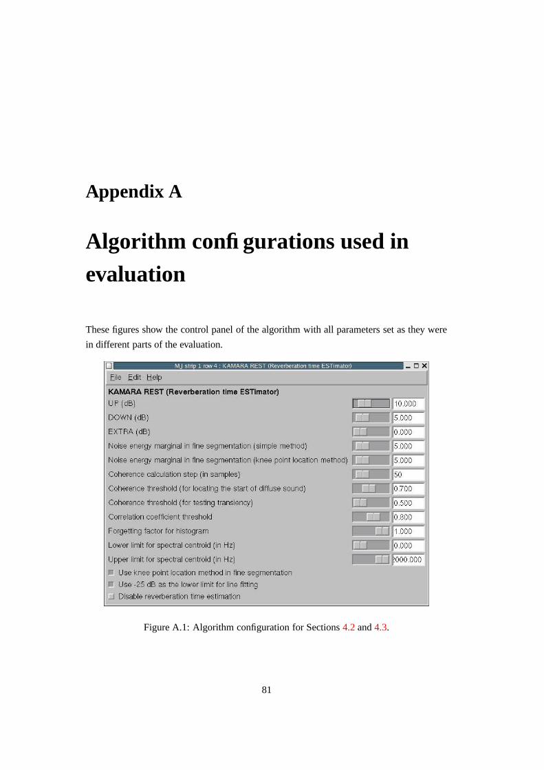
Appendix A
Algorithm configurations used in
evaluation
These figures show the control panel of the algorithm with all parameters set as they were
in different parts of the evaluation.
Figure A.1: Algorithm configuration for Sections 4.2 and 4.3.
81
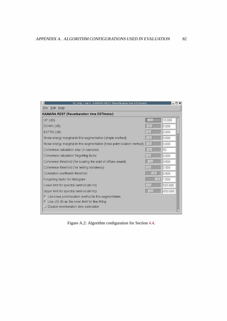
APPENDIX A. ALGORITHM CONFIGURATIONS USED IN EVALUATION 82
Figure A.2: Algorithm configuration for Section 4.4.
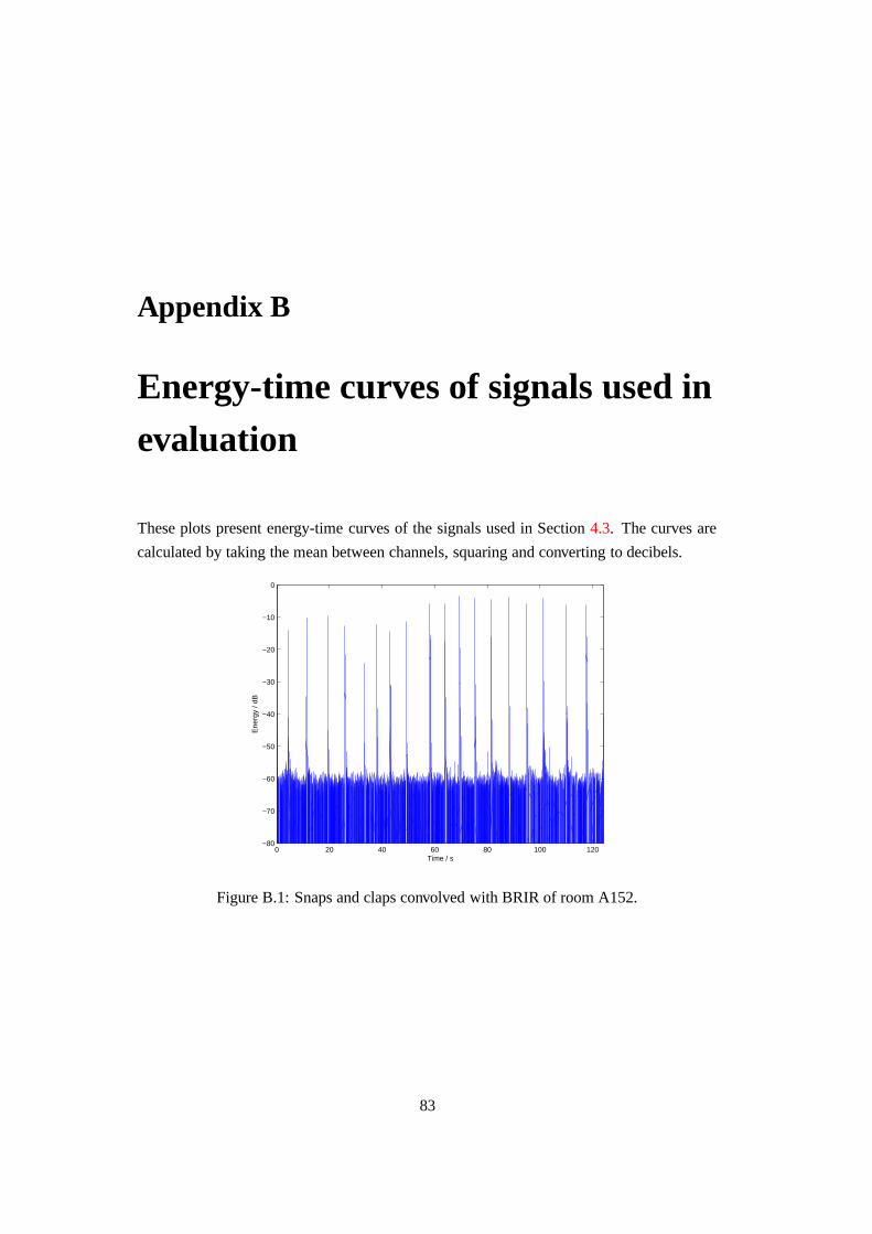
Appendix B
Energy-time curves of signals used in
evaluation
These plots present energy-time curves of the signals used in Section 4.3. The curves are
calculated by taking the mean between channels, squaring and converting to decibels.
0 20 40 60 80 100 120−80
−70
−60
−50
−40
−30
−20
−10
0
Time / s
Ene
rgy
/ dB
Figure B.1: Snaps and claps convolved with BRIR of room A152.
83
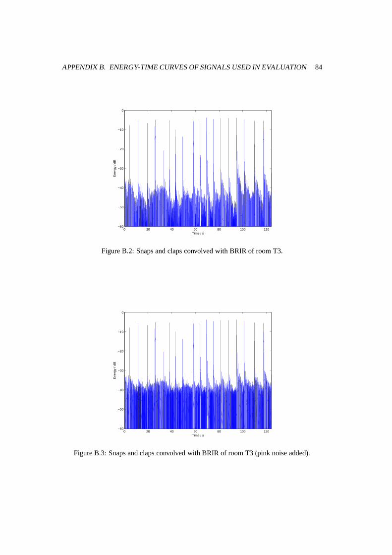
APPENDIX B. ENERGY-TIME CURVES OF SIGNALS USED IN EVALUATION 84
0 20 40 60 80 100 120−60
−50
−40
−30
−20
−10
0
Time / s
Ene
rgy
/ dB
Figure B.2: Snaps and claps convolved with BRIR of room T3.
0 20 40 60 80 100 120−60
−50
−40
−30
−20
−10
0
Time / s
Ene
rgy
/ dB
Figure B.3: Snaps and claps convolved with BRIR of room T3 (pink noise added).
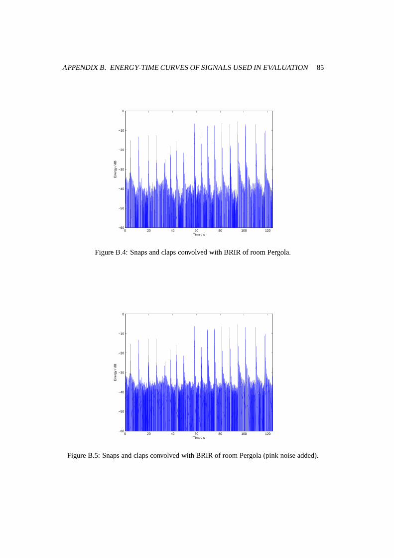
APPENDIX B. ENERGY-TIME CURVES OF SIGNALS USED IN EVALUATION 85
0 20 40 60 80 100 120−60
−50
−40
−30
−20
−10
0
Time / s
Ene
rgy
/ dB
Figure B.4: Snaps and claps convolved with BRIR of room Pergola.
0 20 40 60 80 100 120−60
−50
−40
−30
−20
−10
0
Time / s
Ene
rgy
/ dB
Figure B.5: Snaps and claps convolved with BRIR of room Pergola (pink noise added).