ESTIMATION OF RATES OF RETURN (ROR) ON SOCIAL

PROTECTION INVESTMENTS IN LESOTHO

Stephan Dietrich

Franziska Gassmann

Hanna Röth

Nyasha Tirivayi

28 January 2016

ii

This report was written on behalf of UNICEF Lesotho (LRPS-KMA-2015-9118790). The authors would

like to thank Ousmane Niang, Pierre Mohnen, and the participants of the dissemination workshop

held in Maseru on 28 January 2016, for their useful comments.

iii

Table of Contents

Executive Summary ................................................................................................................................ vi

1. Introduction .................................................................................................................................... 1

2. Background ..................................................................................................................................... 3

Lesotho Country Context ................................................................................................................ 3

Social Protection Landscape ........................................................................................................... 4

3. Direct and Indirect Benefits of Social Protection ............................................................................ 9

Social Protection ............................................................................................................................. 9

International evidence on the effect of social transfers ................................................................. 9

Conceptual Framework ................................................................................................................. 13

4. Study Framework .......................................................................................................................... 14

Reduced Study Framework ........................................................................................................... 14

SPI and Design Parameters ........................................................................................................... 16

Outcome variables ........................................................................................................................ 18

5. Data and Methodology ................................................................................................................. 19

Data ............................................................................................................................................... 19

Limitations..................................................................................................................................... 20

Methodology ................................................................................................................................. 21

6. Analysis and Results ...................................................................................................................... 23

Static simulation ............................................................................................................................ 23

Economic returns and behavioral effects of SPI ........................................................................... 26

Dynamic Simulation ...................................................................................................................... 35

Sensitivity Analysis ........................................................................................................................ 45

7. Conclusion ..................................................................................................................................... 46

References ............................................................................................................................................ 49

Annex .................................................................................................................................................... 53

iv

List of Tables

Table 1. Overview of core Social Protection Programs in Lesotho ......................................................... 5

Table 2: Included SP Programs and Design Parameters ....................................................................... 17

Table 3 Average (monthly) Consumption, Poverty and Inequality in Lesotho ..................................... 22

Table 4 Transfers and Number of Beneficiaries - Static Simulation ..................................................... 24

Table 5 Static Simulation: Relative Change in Poverty and Inequality ................................................. 24

Table 6 Static Simulation: Relative Change in Poverty and Inequality, Urban versus Rural Areas ....... 25

Table 7 Static Simulation: Cost Effectiveness ....................................................................................... 26

Table 8. 2SLS estimation of (log) household consumption per adult equivalent, age 18-69 ............... 28

Table 9. Consumption Effect on School Attendance of Individuals aged 6-24 (IV Probit).................... 31

Table 10. Consumption Effect on Labor Participation of Individuals aged 18-69 (IV Probit) ............... 34

Table 11 Simulation Procedure per Period ........................................................................................... 38

Table 12 Dynamic benefits in periods 5, 10 and 15 .............................................................................. 43

Table 14 Dynamic Benefits with different propensities to consume ................................................... 54

Table 15 Dynamic Benefits of CGP with different targeting mechanisms ............................................ 56

List of Figures

Figure 1: Direct and indirect returns to Social Protection .................................................................... 13

Figure 2: Reduced Study Framework .................................................................................................... 16

Figure 3: Consumption-based Lorenz Curve, 2002/2003 ..................................................................... 22

Figure 4: School Attendance (Age 6-24) - Mean, rural, and urban ....................................................... 29

Figure 5: School Attendance (Age 6-24) - mean, male, female ............................................................ 30

Figure 6: Paid Work (18-70 years) - mean, rural, urban ....................................................................... 33

Figure 7: Paid Work (18-70 years) - mean, female, male ..................................................................... 33

Figure 8: Relative changes in school attendance (% change compared to control group) .................. 40

Figure 9: SPI Effect on Consumption Growth (% compared to control scenario) ................................ 41

Figure 10: SPI Effect on Poverty Headcount ......................................................................................... 42

Figure 11: SPI Effects on Extreme Poverty Headcounts ........................................................................ 42

Figure 13: Rates of Return of Social Protection Instruments ............................................................... 45

Figure 14: Simulated Population Development .................................................................................... 53

Figure 15: Simulated Development of Poverty Headcount .................................................................. 53

Figure 16: SPI monetary returns to education (average consumption per capita effect in Maloti) .... 54

Figure 17: CGP Rate of Return using different Discount Rates ............................................................. 54

Figure 18: CGP Rate of Return using different Targeting Mechanisms ................................................ 56

v

List of abbreviations

BOS Bureau of Statistics Lesotho

CGP Child Grant Program

CMS Continuous Multipurpose Survey

EU European Union

GDP Gross Domestic Product

HBS Household Budget Survey

IMF International Monetary Fund

IV Instrumental Variables

MGSOG Maastricht Graduate School of Governance

MoSD Ministry of Social Development

NISSA National Information System for Social Assistance

NSDP National Strategic Development Plan

NSPS National Social Protection Strategy

OAP Old Age Pension

OVC Orphans and Vulnerable Children

PA Public Assistance

PWP Public Works Program

RoR Rate of Return

SFP School Feeding Program

SP Social Protection

SPI Social Protection Investments

UNICEF United Nations Children’s Fund

WDI World Development Indicators

WFP World Food Program

WHO World Health Organization

vi

Executive Summary

Compared to other low-income countries, Lesotho is one of the leaders in social protection. It is at the

forefront of moving towards a social protection systems approach in Sub-Sahara Africa and beyond.

The National Social Protection Strategy (NSPS) 2014/15-2018/19 (Government of the Kingdom of

Lesotho, 2015) represents the Government’s vision and ambitions for the coming years to address the

risks and challenges over the life-course to protect its citizens and particularly the poor and vulnerable

Basotho. The implementation of the envisaged core social protection programs for children, the

elderly and poor adults, supplemented by complementary programs in other sectors has the potential

to significantly reduce the extent and depth of poverty and provide citizens with the means to improve

their livelihoods in the short and long term.

It is estimated that the implementation of the core programs of the NSPS will cost four percent of GDP

at full coverage (Government of the Kingdom of Lesotho, 2015). Although the analysis has shown that

the strategy is affordable, four percent of GDP represents a considerable amount of national

resources. In order to garner continued political and financial support for the implementation of the

NSPS, it is essential to build strong economic arguments, proving that the investment is worthwhile in

terms of expected benefits in the future.

The aim of this study is to estimate the Rate of Return (RoR) on Social Protection Investments (SPI) in

Lesotho, thereby generating evidence to support the advocacy for social protection in Lesotho and

assisting relevant ministries in planning the allocations for SP instruments. The primary focus of the

study is the Child Grant Program (CGP). The CGP targets extremely poor households with children

aged between 3 and 17 years. The net benefits of the CGP are compared with the Old Age Pension

program (OAP), the school feeding program (SFP) and with a combined package of CGP and OAP.

Non-contributory social transfers directly affect household disposable income, and as such household

consumption. However, social transfers also affect household behavior through income and non-

income effects. Additional and/or secure income encourages households to invest in health,

education, livelihoods and productive activities. The study thus builds on a framework assuming both

direct and indirect benefits through increased consumption due to social protection investments (i.e.

poverty reduction and human capital accumulation).

The methodology applied in this study consists of three main elements. First, a static simulation is

implemented, revealing the direct effects of the increase in household consumption on poverty and

inequality. Secondly, different empirical models are used to estimate the relationship between

household consumption and school attendance, school attainment and household consumption, and

vii

household consumption and labor market participation. Finally, a dynamic simulation model was

constructed in order to predict the effects of social transfers over a period of 15 years. The simulation

procedure remains the same in each period. Eligible beneficiaries of the respective SP instrument

receive the benefits, which increases their consumption levels with 80% of the transfer values. Based

on the new consumption level, the likelihood of school age children to attend school is predicted.

Subsequently, the educational attainment is updated depending on whether children attended

school. The new consumption levels are calculated as the sum of the previous consumption level plus

the direct effect (transfers) and the behavioral benefit. Fertility and mortality rates are integrated into

the simulation model in order to reflect demographic changes over time. The dynamic simulation

compares the outcomes of the programs to a scenario without SPI. Therefore, the focus is not on

predictions of outcome variables in future periods, but rather on the relative development in

outcomes compared to the control scenario. The Rate of Return compares the net present value of

benefits of an intervention to the net present value of the costs of this intervention.

The analysis is based on the nationally representative Household Budget Survey 2002/2003. Further,

data on demographic projections was obtained from the Bureau of Statistics of Lesotho and from the

World Health Organization to simulate demographic developments over the time period of the

analysis.

With respect to the direct effects on poverty and inequality, the largest reduction in poverty

headcount can be observed for OAP followed by SFP and CGP. For the CGP no immediate effect on

the poverty headcount can be measured. This is due to its focus on extremely poor households that

do not graduate out of poverty with the transfer as the gap is too large. However, the potential effects

of the CGP become evident when considering extreme poverty outcomes. The simulation suggests

that CGP reduces the extreme poverty headcount by 20% compared to a scenario without SPI. The

results of the static simulation also suggest that the CGP is the most cost-effective program as it would

generate the largest reductions in outcomes for each percent of GDP invested. According to the static

simulation, investing 1% of GDP in the CGP would generate a reduction of 15.3% in extreme poverty,

which is about five times the size of the OAP program effect at the same cost.

Based on the empirical models, which are based on the situation in 2002, the estimates imply positive

returns to education of an additional year of schooling of 9%, which is close to the international

standard of approximately 10% (Psacharopoulos and Patrinos 2004). The effect of household

consumption on school attendance is also positive. At the national level, a 10 percent increase in

household consumption is associated with a 1.1 percentage point higher probability of a child

attending school. The findings suggest that household consumption positively affects school

viii

attendance rates in Lesotho. This implies that SP instruments that increase household consumption

levels likely improve education outcomes and therefore contribute to human capital development in

Lesotho. The results further show that household consumption has a positive effect on labor market

participation. At national level, a 10 percent increase in household consumption level is associated

with a 1.6 percentage point increased probability of labor participation for individuals aged 18 to 69.

Overall, the findings suggest that SPI that increase household consumption levels (income) potentially

raise participation in the labor markets in Lesotho.

The dynamic simulation model is applied to examine the effects over time including the behavioral

effects through increased school attendance and higher school attainments. Thus, the SP effects are

simulated over a 15 years’ time range. All three programs affect school attendance and educational

attainments positively. School attendance rates of individuals between 6 and 24 years increased

strongest for the CGP scenario and the combination of CGP and OAP. The CGP school attendance rate

increased by 5% in the first period, which grows up to an annual increase of more than 12% in period

15 compared to the control scenario. As the SP effects sum up over time, an exponential growth in

school attendance rates can be observed. As a consequence, after 15 periods the working-age adults

dispose of a 2% higher school attainment in the CGP scenario as compared to the control scenario.

The OAP effect on school attendance is markedly smaller. Despite the larger transfer values of OAP

the effect is lower as it is not specifically targeted at children. The combination of CGP and OAP further

increases school attendance rates, however, adding only little to the CGP effect.

The effect of the SFP on school attendance is smaller than the CGP effect and increases up to around

7% at the end of the simulation period. Yet, the annual growth rates are smaller than for the other

programs. This is due to the SFP assignment to children that are already enrolled in school with thus

little scope to further increase attendance rates. However, it has to be noted that the potential effects

of SFP on aspects such as school performance or health cannot be regarded in the model. These effect

pathways could have important impacts on school attainments and may result in underestimation of

the educational effects of SFP in the simulation model.

The analysis of the returns to education suggests that an additional year of schooling increased

consumption levels on average by 9% in 2003. At the same time results of the dynamic simulation

model show that CGP increased the number of years of schooling on average by 2% per year. This

highlights the potential of SPI to generate large returns in future periods. However, the results also

showed that school attainments tend to be low in Lesotho and that the education effects especially

on the extremely poor need more time to unfold their full returns.

ix

This results in initially negative RoR, which slowly start to improve and turn positive after 10 periods

for the CGP. The simulation results suggest that from period 10 onwards the net benefits of the CGP

exceed the costs. The RoR of OAP and SFP remain negative throughout the simulation, but show a

positive trend. This finding is related to the fact that both programs have universal targeting

mechanisms and do not particularly benefit the extremely poor. Secondly, beneficiaries either already

attend school (SFP) or left school age long ago (OAP). Thus, their scope to generate returns through

school attendance is much lower compared to CGP resulting in lower behavioral benefits.

The findings suggest large program effects on poverty and inequality outcomes. Simulating the CGP

on the national level reduced extreme poverty by more than 20% per year and reduced inequality by

up to 7%. This indicates the potential of CGP for poverty reductions in Lesotho. Taking all future

returns into account, the educational benefits exceed all cost including transfers and operational costs

after 10 periods. This underpins the power of SPI for educational but also welfare developments in

Lesotho. On top of that, additional returns through health and agricultural investments and increasing

tax revenues are not considered in this study. Therefore, the results might only reflect a lower bound

estimate of the full potential of social cash transfers.

As a model can never cover the entire set of SPI linkages, it needs to be born in mind that simulation

models are always a simplification of reality. The study has a number of particular limitations that

need to be born in mind when interpreting the results. Due to the limitations of the HBS 2002/2003

data, not all potential indirect benefits of social transfers could be incorporated in the model. Effects

through improved health or investments in productive activities are not considered, which may be

particularly important for the OAP. Therefore, the resulting rates of return are likely an

underestimation of the actual achievements. Furthermore, the economic and social situation in

Lesotho has changed considerably since 2002/2003. For example, school attendance and highest

education achievements have increased considerably over the last decade. Nonetheless the models

show how specific aspects of SPI pathways generate monetary returns over the long term.

It is recommend to repeat the present analysis once more comprehensive and more recent household

survey data are available. Particularly the inclusion of other transmission channels next to education

would add value and provide additional insights in the potential benefits and the respective RoR in

the long term. Furthermore, information such as access to services and infrastructure would allow a

more detailed analysis of the returns of SPI which goes beyond the national average and provide

insights into policy areas that need to be strengthened in order to maximize the impact of SPI. The

BOS is keen to improve their data collection and adjust the survey instruments such that they better

serve the overall needs for regular analysis and evaluation of social protection policies.

1

1. Introduction

Compared to other low-income countries, Lesotho is one of the leaders in social protection. It is at the

forefront of moving towards a social protection systems approach in Sub-Sahara Africa and beyond.

The National Social Protection Strategy (NSPS) 2014/15-2018/19 (Government of the Kingdom of

Lesotho, 2015) represents the Government’s vision and ambitions for the coming years to address the

risks and challenges over the life-course to protect its citizens and particularly the poor and vulnerable

Basotho. The implementation of the envisaged core social protection programs for children, the

elderly and poor adults, supplemented by complementary programs in other sectors has the potential

to significantly reduce the extent and depth of poverty and provide citizens with the means to improve

their livelihoods in the short and long term. Simulations for Lesotho indicate that the implementation

of a set of core programs could reduce the poverty rate by 15 percent and the poverty gap by 40

percent (Government of the Kingdom of Lesotho, 2015:34).

It is estimated that the implementation of the core programs of the NSPS will cost four percent of GDP

at full coverage (Government of the Kingdom of Lesotho, 2015). Although the analysis has shown that

the strategy is affordable, four percent of GDP represents a considerable amount of national

resources. In order to garner continued political and financial support for the implementation of the

NSPS, it is essential to build strong economic arguments, proving that the investment is worthwhile in

terms of expected benefits in the future. Lesotho currently spends nine percent of its GDP on social

protection programs (World Bank, 2013), which is well above the average of most developing

countries. However, there is considerable scope for coordination and harmonization of existing social

protection programs. To achieve a more efficient allocation of funds, evidence is required to guide

policymakers in their investment decisions. Using the existing social protection funds more efficiently

could benefit the poor and strengthen the efforts to mitigate the consequences of pervasively high

poverty rates in Lesotho.

The aim of this study is to estimate the Rate of Return (RoR) on Social Protection Investments (SPI) in

Lesotho. The objective of the analysis is to generate evidence to support the advocacy for social

protection in Lesotho and to assist relevant ministries in planning the allocations for SP instruments.

This project has been commissioned by UNICEF in the framework of the EU-funded Support

Programme to Orphans and Vulnerable Children - Phase 2, and implemented by Maastricht University,

Maastricht Graduate School of Governance (MGSOG). The analysis compares economic benefits of SP

investments based on individual increments with the economic program costs. The estimation will

complement existing impact evaluation results by analyzing the returns to SP in the mid- and long

term perspective. The primary focus of the study is the Child Grant Program (CGP), which was

2

implemented on a pilot basis. The CGP targets extremely poor households with children aged between

3 and 17 years. The net benefits of the CGP are compared with the Old Age Pension program (OAP),

the school feeding program (SFP) and with a combined package of CGP and OAP. In this study the RoR

of the program is simulated ex ante at the national level providing evidence for the case of a national

implementation of the program.

The remainder of the report is structured as follows: Section two describes the economic country

context and the existing landscape of social protection in Lesotho. The conceptual framework linking

social protection with development and economic growth is introduced in section three. Section five

elaborates the study framework guiding the present analysis and section five introduces the data used.

Section six presents the results of the quantitative analysis and section seven concludes.

3

2. Background

Lesotho Country Context

Lesotho is a country with a population of 2.1 million (World Bank, 2014)1 and it is entirely surrounded

by South Africa in the South Eastern part of the country. It has been independent since 1966. The

geography is mainly characterized by mountainous and rural areas. Lesotho is one of the poorest

countries in southern Africa and one of the most unequal economies in the world (World Bank, 2015b).

The main sectors driving the economy are the textile industry and mining activities. In general,

economic activity is limited and informal employment is prevalent with 72 percent of those employed

working in the informal sector (Olivier, 2013). Over the last ten years, the economy has been growing

at an average of four percent annually (IMF, 2015). Yet, economic growth has not been pro-poor,

which is also due to a strong bifurcation of the economy in formally and informally employed sectors.

The incidence and depth of poverty and the level of inequality are far above average for a country

characterized by this level of growth.

The incidence of poverty has remained high over the last decade with an estimated poverty rate of 57

percent in 2010 (World Bank, 2013). There are several reasons that have contributed to persistently

high poverty rates. The depth of poverty, estimated at 30 percent of the poverty line, makes it difficult

for many households to graduate out of poverty. In addition, derailing factors such as the HIV/AIDS

epidemic and environmental and price shocks are other important sources for persistently high

poverty rates and a major source for households’ vulnerability to poverty (World Bank, 2015b).

The population of Lesotho faces numerous challenges, particularly regarding income insecurity and

health. In 2013, the value of the Human Development Index was 0.486 (UNDP, 2014), which is low in

international comparison. While the value has increased from 0.443 in 1980, the overall increase of

the index hides the development of individual factors. While the average number of years of schooling

and GNI per capita have increased, life expectancy at birth has decreased by 4.4 years (UNDP, 2014).

The decline in life expectancy and the general incidence of poor health outcomes are due to the high

prevalence of HIV/AIDS and high rates of tuberculosis infection among those living with HIV/AIDS,

which are particularly high in Lesotho (World Bank, 2015b). Considering the HIV/AIDS prevalence rate

of 23 percent among adults, it is evident that this affects the ability of the population to benefit from

growth on the one hand and the provision of productive labor on the other hand. Jointly, these

1 Retrieved from data.worldbank.org

4

difficulties inhibit Lesotho and its population from enhancing inclusive growth and well-being and

from fostering human development.

Income inequality is another challenge. The Gini coefficient was estimated to be 0.53 in 2010 (World

Bank, 2013), indicating that enhancing equality needs to be a central component of poverty alleviation

efforts. However, it is important to note that countries with a Human Development Index similar to

Lesotho like Senegal and Uganda face even higher levels of inequality (World Bank, 2013). The

population of Lesotho further face high levels of malnutrition as evidenced by the latest Demographic

and Health Survey 2014, which states that 33 percent of all children under the age of five are stunted

and 11 percent are severely stunted (Ministry of Health, 2015). The National Strategic Development

Plan (NSDP) 2012/13 – 2016/17 (Government of Lesotho, 2015) is an important development

framework that entails goals relating to employment, infrastructure, democratic governance,

improvement of health and technology and innovation. The NSDP was adopted in 2012 as part of the

ambition to realize Lesotho’s “Vision 2020”. It underlines the importance of social protection and

suggests considering the reduction of vulnerability and enhancing the coverage and efficiency of social

protection as a key component of national development initiatives.

Social Protection Landscape

The underlying goal of SPI in Lesotho is to provide a strong safety net for vulnerable groups. While still

belonging to the category of least developed countries, Lesotho shows one of the highest rates of

social protection expenditure in Africa (ILO, 2012). In 2010/2011 about 16 percent of Government

expenditures were used for SP, which was equivalent to 9 percent of GDP (World Bank, 2013:22). This

amount, however, includes a large variety of different transfers and programs of which not all would

necessarily be classified as social protection (for example, the tertiary bursary scheme) (Khondker &

Freeland, 2014a). Core social assistance programs accounted for 4.5 percent of GDP or 8 percent of

public expenditure (World Bank, 2013:22). Lesotho spends considerably more on social assistance

than most other countries in the region, where social safety net expenditures range between 0.2

percent of GDP in Zambia and 2.2 percent in Botswana or Swaziland (World Bank, 2013:23). Various

social protection programs are in place and several ministries are in charge of their implementation.

Details of the core programs, expenditures and ministries in charge are summarized in Table 1 and the

programs included in the simulation are outlined in more detail below. About 76 percent of all social

assistance expenditures are currently spent on Old Age Pensions (OAP) (2.39 percent of GDP) and

School Feeding Programs (SFP) (1.05 percent of GDP). Other key programs include the Child Grant

Program (CGP), Orphans and Vulnerable Children (OVC) Bursary Program, Public Assistance (PA), and

Public Works Programs (PWP).

5

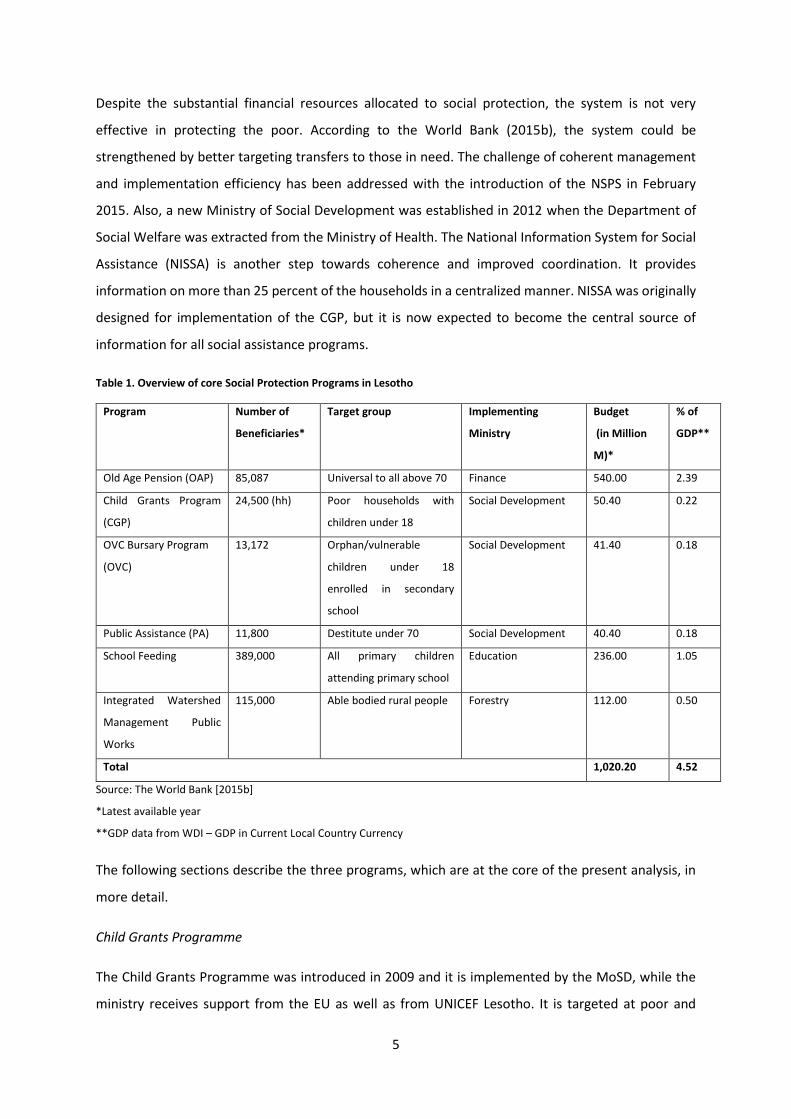
Despite the substantial financial resources allocated to social protection, the system is not very

effective in protecting the poor. According to the World Bank (2015b), the system could be

strengthened by better targeting transfers to those in need. The challenge of coherent management

and implementation efficiency has been addressed with the introduction of the NSPS in February

2015. Also, a new Ministry of Social Development was established in 2012 when the Department of

Social Welfare was extracted from the Ministry of Health. The National Information System for Social

Assistance (NISSA) is another step towards coherence and improved coordination. It provides

information on more than 25 percent of the households in a centralized manner. NISSA was originally

designed for implementation of the CGP, but it is now expected to become the central source of

information for all social assistance programs.

Table 1. Overview of core Social Protection Programs in Lesotho

Program Number of

Beneficiaries*

Target group Implementing

Ministry

Budget

(in Million

M)*

% of

GDP**

Old Age Pension (OAP) 85,087 Universal to all above 70 Finance 540.00 2.39

Child Grants Program

(CGP)

24,500 (hh) Poor households with

children under 18

Social Development 50.40 0.22

OVC Bursary Program

(OVC)

13,172 Orphan/vulnerable

children under 18

enrolled in secondary

school

Social Development 41.40 0.18

Public Assistance (PA) 11,800 Destitute under 70 Social Development 40.40 0.18

School Feeding 389,000 All primary children

attending primary school

Education 236.00 1.05

Integrated Watershed

Management Public

Works

115,000 Able bodied rural people Forestry 112.00 0.50

Total 1,020.20 4.52

Source: The World Bank [2015b]

*Latest available year

**GDP data from WDI – GDP in Current Local Country Currency

The following sections describe the three programs, which are at the core of the present analysis, in

more detail.

Child Grants Programme

The Child Grants Programme was introduced in 2009 and it is implemented by the MoSD, while the

ministry receives support from the EU as well as from UNICEF Lesotho. It is targeted at poor and

6

vulnerable households that are selected according to a combined assessment of a proxy means test

and community validation, given that households belong to NISSA category 1 or 2 (thus considered

extremely poor). The transfer is paid on a household level and the amount depends on the number of

children in a household; it ranges from 360 to 750 Maloti per quarter. Previously the transfer amount

did not depend on the number of children and each eligible household received a flat amount of 360

Maloti per quarter. According to a recent report, approximately three hours in total are spent walking

to pay points and back (Pellerano et al., 2014).

Pellerano et al. (2014) observed that households received the intended amounts throughout the

evaluation period. However, these were provided irregularly and in large portions, which does not

correspond with the intention to offer a predictable and regular form of financial support. In general,

beneficiary households were found not to be aware of specific amounts and timing of future payments

(Pellerano et al., 2014).

Evidence from the impact evaluation of the Child Grant Program indicates that the program has had

beneficial outcomes particularly with respect to child well-being, but also with respect to outcomes

outside the direct realm of the program. Beneficiary households increased education-related spending

of pupils by 38 percent on average. The program also had a positive effect on school enrolment and

retention. With respect to health-related outcomes, birth registration increased by 37 percentage

points and the illness incidence of under-5 children decreased by 15 percentage points. Furthermore,

beneficiary households were more food secure. The positive effect on household livelihoods is

evidenced by the increased share of households using crop inputs. Moreover, beneficiary households

were better protected against shocks and as such did not have to refer to disruptive coping strategies.

The analysis of local multiplier effects with the LEWIE model confirmed the potential of cash transfers

of generating large multiplier effects. It is estimated that each Loti transferred to a poor household

can raise local income by M2.23 (Ministry of Social Development, 2014).

Old Age Pension

The Old Age Pension program was introduced in 2004 and is currently the largest social assistance

program in place (Olivier, 2013). It provides a universal non-contributory pension to all individuals

above the age of 70, excluding only former civil servants who receive a higher government pension.

The current transfer amount is 500 Maloti (USD 33) per month and the number of beneficiaries

increased by 30 percent between 2004 and 2011.

Based on a recent review conducted by the World Bank (2015b), there are currently about 85,000

beneficiaries. Interestingly, though, this number exceeds the actual number of citizens aged 70 or

7

older, pointing at potential implementation problems and/or lack of administrative monitoring.

Families of deceased pensioners often continue to receive benefits, which is facilitated by the fact that

authorities not always insist on receiving a proof of life. Further factors contributing to pensions

allocated to ineligible citizens are the lack of internal controls allowing staff members to generate

artificial records and collect benefits, and the lack of registration and birth certificates, which

facilitates reporting a higher age at application. Finally, beneficiaries are not always eliminated from

the records upon death due to technical constraints (World Bank, 2015b). Although the application

process for the Old Age Pension is rather straightforward and flexible, the amount of time and costs

involved in collecting payments and the labour intensive distribution process render the system less

efficient.

Even though only an estimated six percent of the poor are older than 64, the OAP has important

effects on household consumption and poverty. Beneficiaries hardly live in isolation and as such the

OAP benefits individuals living in the same household. Evidence indicates that the OAP increased food

security as most of the money is spent on food (Chroome, 2007; Ayala Consulting, 2011 – both quoted

in World Bank, 2013). Children also benefit indirectly from the OAP as an estimated 20 percent of the

pension is spent on dependent orphan children (Ayala Consulting, 2011 in World Bank 2013).

School Feeding Programme

Almost 400,000 children attending primary public schools benefit from a daily lunch at school. The

School Feeding Program targets all children attending public primary school intending to enhance both

educational and health outcomes. It is implemented by the Government of Lesotho with support from

the World Food Program (WFP). Children in school receive a lunch during 180 days per year. In areas

supported by the WFP, children also benefit from a mid-morning snack. In most cases the food is

prepared at school by local caterers, except in cases where schools lack the necessary facilities. In the

latter case, the food is prepared in the home of the caterer.

In kind transfer programs, such as the SFP, are often not the most cost-efficient ways to transfer

benefits to eligiblie households. This is also the case for the SFP in Lesotho. It is estimated that more

than 50 percent of the total program costs are operational costs such as food delivery and storage, or

catering. The value of the actual meal is about 203.4 Maloti per year, while total costs of the

Government-run program are 637 Maloti per child per year (World Bank, 2013).

Even though eligiblity for the SFP is universal, the program is slightly progressive given that an

estimated 43 percent of the primary school pupils are from the poorest 40 percent of the population.

It is an example of broad targeting with the aim to increase access to public services to the poor. The

8

SFP has positive impacts on school enrolment, attendance and reduces drop out rates (Motseng

Logistics Services, 2011; Haag et al. 2009, both in World Bank, 2013).

9

3. Direct and Indirect Benefits of Social Protection

Social Protection

The main objectives of social protection are to guarantee human rights (social, political and economic),

promote human development and encourage economic growth. Investments in social protection

contribute to economic growth and territorial development2, reduce poverty and inequality across

and between groups and contribute to the quality of governance by strengthening institutions. Social

protection also plays a role for employment policies and basic services. It contributes to the protection

and accumulation of human and physical capital and acts as stabilizer for effective demand. It provides

means and resources to solve poverty traps by easing credit constraints and covering transaction

costs. These features are essential for the successful implementation of effective employment policies

and the achievement of universal access to basic services, such as education and health, pointing at

the complementarity of social protection and other social policies.

The design of Social Protection policies covers a wide range of features, depending on the specific

priorities and context of the community where they are implemented. One key distinction needs to

be made between social insurance programs which are (mainly) financed through contributions of the

beneficiaries and thus granted to those who contribute, and social assistance programs provided on

the grounds of certain income or household criteria irrespective of any contributions made in the past.

Both types of designs can affect well-being and economic growth if implemented well, yet the most

financially deprived and vulnerable groups are commonly targeted with social assistance programs.

The following review as well as the analysis focus on the latter group of policies, thus non-contributory

transfers financed by the government or supported by international donors. Further, cash transfers

can be designed to be conditional on the fulfillment of a certain behavior of the recipient households,

e.g. regular school attendance or health inspection, while others are unconditionally provided to all

eligible households or individuals.

International evidence on the effect of social transfers

Non-contributory social transfers directly affect household disposable income and, subject to the

marginal propensity to consume, the level of consumption. Simulations for Lesotho indicate that the

implementation of a set of core programs could reduce the poverty rate by 15 percent and the poverty

gap by 40 percent (Government of the Kingdom of Lesothos, 2015:34). The increase in disposable

income as a result of social transfers affects household behavior and economic performance at

2 See e.g. Alderman & Yemtsov (2012); Cherrier, Gassmann, Mideros & Mohnen (2013); Barrientos (2012).

10

different levels. A substantial amount of research has been conducted in order to investigate and

emphasize these effects and potential enhancements of existing transfer schemes.

An underlying question often raised in this context is to what extent investments in social protection

transfers have an effect on economic growth. As Alderman & Yemtsov (2012) point out, early studies

assumed that by shifting resources to less productive shares of the population and by providing

disincentives to work or education, cash transfers would be an inefficient approach to poverty and

inequality with negative economic effects. Furthermore, rising inequality was not considered

problematic when weighed against efficiency and economic growth (Alderman & Yemtsov, 2012). At

a later stage, when long term data on new schemes became available it was found that such

investments could be beneficial for the overall economy and that disincentives were not substantial if

certain precautions were made (Barrientos & Scott, 2008). For instance, Castells and Himanen (2002)

found that cash transfers can enhance innovation and thereby increase competitiveness within and

across communities. Alderman and Yemtsov (2012) base their analysis on the potentially productive

effects achieved by well-designed cash transfer programs. When distributing regular and sufficient

resources to vulnerable groups, these may be invested in activities enhancing the level of education

or the opportunity for employment and investment. Here, four channels for these productive effects

are identified. According to their concept, social transfers may affect the economy through human

capital investments, by substituting for a lack of access to credit and thereby stimulating investment,

through labor market improvement due to pensions and through local spillover effects. These effects

can occur at the level of the household, within a community and at the national level.

Further evidence was provided by Barrientos (2012). With a focus on social transfers in developing

countries, Barrientos (2012) investigated different mechanisms how these policies affect growth at

the micro level. He also referred to the productive capacity of households, claiming that one should

focus on economic growth within the vulnerable group rather than the economy as a whole. He

emphasized that policies should be designed with a priority to enhance the productive capacity of

households, by stimulating human, physical and financial asset accumulation. In his study it is further

outlined that certain characteristics of the transfers are decisive. For instance, it has been found that

a regular and reliable payment of benefits is crucial for a sustainable use by beneficiaries and the

transfer amount needs to be sufficient to ensure the productive capacity while it may not be too high,

causing recipients to rely on them rather than making investments.

As Dercon (2011) points out, it is crucial for social protection mechanisms to be integrated with

policies promoting improvement of services available to the population, such as health and education

facilities and a stable formal labor market. The following sections present recent evidence on effects

11

of social transfers on education, health and labor and on local multiplier effects as well as evidence on

rates of return that have been estimated.

Education

International evidence is highly conclusive about a positive effect of social transfers on school

attendance. Social transfers increase the disposable income and, by reducing cost barriers, increase

school enrolment and attendance.3 Meng and Ryan (2009) evaluated the Food for Education (FFE)

program in Bangladesh seven years after its implementation and through propensity score matching

they were able to show that the school participation rates of recipient children were higher than those

of non-recipients by approximately 15 to 27 per cent. The number of years spent in school was also

found to be higher by 0.7 to 1.05 years. Here the benefit was paid per month given that the child

attended school at the time. In this context, Schady and Arujo (2006) found that even if conditions are

just assumed and not specified or monitored, beneficiary households tend to adjust their behavior.

They observed the case of the Bono de Desarrollo Humano (BDH) benefit in Ecuador which had

significant positive effects on school enrollment (10 pp.) and significant negative effects on child work

(17 pp). Approximately twenty-five per cent of all households in the sample believed eligibility was

tied to a certain behavior. When comparing beneficiaries and non-beneficiaries in this group and in

the group not assuming any conditions, the effect on school enrollment was only found to be

significant for those who perceived the benefit to be conditional (Schady & Arujo, 2006). Their study

thus demonstrated the effect that particularly conditional cash transfers can have on school

enrolment and thus human capital accumulation.

Health

The second behavioral income effect of social protection is on the health status of the population.

Several studies provide evidence about the positive effects of different social transfers on food

consumption and health. As Adato and Bassett (2009) claim, there are three likely mechanisms for

cash transfers to have positive sustainable effects on the health of recipients. Transfers can cover costs

incurred for counselling or treatment, they can indirectly affect health through enhancing the amount

and value of food available to the household, and they can encourage healthy behavior through

conditional transfer designs. Miller, Tsoka & Reichert (2008) analysed the Mchinji Cash Transfer

program in Malawi and found that recipients were more likely to be provided with care than non-

recipients and children were found to be ill in a significantly smaller number of cases, by 13 percentage

points. Further, the Progresa program in Mexico was found to incentivize particularly the health of

3 See Baird et al. (2013) for a systematic review.

12

children as the share of infants taken to growth monitoring visits significantly increased by 5.5 to 13.3

percentage points (Gertler, 2000). However, the main determinants of a positive effect on health are

the size and periodicity of the transfer, the target group and complementary investments.

Labor Supply

Thirdly, changes in disposable income due to social transfers may affect labor supply as they generate

the opportunity to take up work (e.g. covering transportation costs and reducing financial and care

constraints) or to change jobs as the person may afford a longer search period. International evidence

suggests that social transfers have a positive effect on labor supply, while reducing child work. As

mentioned above, early work on the relation between cash transfers and labor supply assumed that

the effect would be negative given the alternative source of income. Today the evidence is more

diverse and positive as well as negative effects have been demonstrated. While certain programs

specifically aim at promoting employment, others have indirect effects on labor supply (Samson,

2006). For instance, public work schemes can generate seasonal, short term employment while the

long-term effects are debated (Chirwa et al., 2004). As Devereux and Solomon (2006) found, a public

works scheme in Argentina (Jefes y Jefas de Hogar) successfully enabled beneficiaries to eventually

secure long-term employment outside of the program. Indirect effects are expected when other types

of transfers lead to improved education, for instance. Tembo et al. (2014) investigated a pilot cash

transfer scheme in Zambia and found that to a large extent benefits were used to hire labor which

facilitated higher productivity of the land and local employment while generating larger amounts of

resources for the household. Similarly, the former program ‘Progresa’ in Mexico appeared to increase

employment opportunities on the community level, benefitting recipients and non-recipients (Barber

& Gertler, 2008). As Samson (2009) emphasizes, one of the most important mechanisms in the labor

effect of cash transfers is the enhancement of social risk management. Households are more likely to

be able to maintain the productive capacity in the case of economic shocks and they can afford a more

effective job search when they are not forced to accept any type of employment due to the need for

immediate relief (Samson, 2009).

Additional effects relate to households’ investments in child wellbeing and productive activities that

raise human and physical capital and foster labor productivity. Moreover, social transfers are likely to

be spent locally, thereby generating local and regional economic multiplier effects. 4

4 See for further evidence on the benefits of social transfers, e.g., Arnold et al. (2011); Schady & Araujo (2006); Bourguignon, Ferreira & Leite (2003); Schady & Rosero (2008); Barrientos & Scott (2008); World Bank (2015c).

13

Conceptual Framework

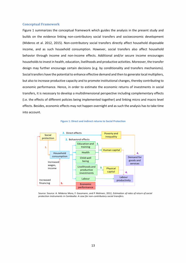
Figure 1 summarizes the conceptual framework which guides the analysis in the present study and

builds on the evidence linking non-contributory social transfers and socioeconomic development

(Mideros et al. 2012, 2015). Non-contributory social transfers directly affect household disposable

income, and as such household consumption. However, social transfers also affect household

behavior through income and non-income effects. Additional and/or secure income encourages

households to invest in health, education, livelihoods and productive activities. Moreover, the transfer

design may further encourage certain decisions (e.g. by conditionality and transfers mechanisms).

Social transfers have the potential to enhance effective demand and then to generate local multipliers,

but also to increase productive capacity and to promote institutional changes, thereby contributing to

economic performance. Hence, in order to estimate the economic returns of investments in social

transfers, it is necessary to develop a multidimensional perspective including complementary effects

(i.e. the effects of different policies being implemented together) and linking micro and macro level

effects. Besides, economic effects may not happen overnight and as such the analysis has to take time

into account.

Figure 1: Direct and indirect returns to Social Protection

Source: Source: A. Mideros Mora, F. Gassmann, and P. Mohnen, 2012, Estimation of rates of return of social protection instruments in Cambodia: A case for non-contributory social transfers.

14

4. Study Framework

The Rate of Return (RoR) compares the net present value of benefits of an intervention to the net

present value of the costs of this intervention. This study uses micro simulations to analyze how the

RoR of different SPI develops over time. More precisely, we simulate the RoR over a period of 15 years

to regard for the returns to behavioral effects such as education, which typically requires some time

to unfold their full benefits. Microsimulations is a technique for the analysis of economic and social

policies at the micro level when the focus is on distributional effects rather than average or aggregate

level.

Therefore the simulation results complement existing impact evaluation results in several ways: most

importantly the study extends the evidence horizon by adding a long-term, forward looking

perspective in addition to rather short-term, back ward looking evaluation studies. Furthermore, it

expands the scope of SPI from pilot areas to a hypothesized nationwide implementation, which

addresses concerns of external validity of impact evaluations. In addition, simulation models can be

used to examine to what extent different targeting procedures, transfer values, or complementary

interventions could change the program outcomes.

The study focuses on benefits at the individual and household level including direct and behavioral

effects of SPI. Income levels approximated by household consumption are used to monetarize effects

and to quantify returns using one common base for the aggregation of benefits. The costs for SPI are

derived from impact evaluation results and different cost assessments.

As a model can never cover the entire set of SPI linkages it needs to be born in mind that simulation

models are always a simplification of reality. Nonetheless the models show how specific aspects of SPI

pathways generate monetary returns in future periods. Therefore, the analysis is a scenario based ex-

ante simulation that sheds light on the cost-effectiveness of different SPI on the national level.

Reduced Study Framework

The applied study framework is determined by the data availability. The linkages to be drawn between

SPIs and other aspects of socio-economic development need to be covered in the data. For example

to analyze the returns to investment in SPI through human capital effects, data on educational

outcomes and health variables are required.

Typically data limitations do not allow simulating the complete conceptual model but only those

aspects sufficiently covered in the data. The data availability and limitations will be discussed in more

15

detail in section five. However, it is important to note that the outcomes of this study only refer to a

reduced model that cannot regard all SPI effect pathways as explained in previous section.

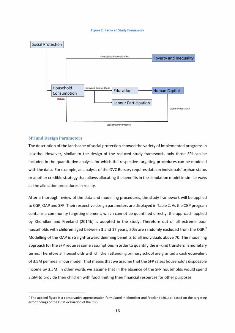
Figure 2 displays the reduced study framework adapted to the HBS 2002 data. The framework draws

linkages between SP, human capital and labor outcomes by modelling the behavioral responses of an

income increase on education and labor participation decisions. Impacts through agricultural

investments or improved health outcomes cannot be simulated with the HBS 2002 data. This means

that the analysis of the RoRs only refers to the reduced model, more specifically, it only considers

effects achieved through increased schooling, disregarding potentially important aspects such as

health, productive assets and agricultural impacts. Thus the reduced study framework could lead to a

lower bound estimation of the RoR, which needs to be kept in mind for the interpretation of the

results.

The proposed methodology to estimate the RoR follows the approach presented in Mideros et al.

(2012, 2015). Within the framework the national economic performance is kept constant and the RoR

is simulated based on consumption returns. In the model macro-economic and structural conditions

affect both the situation with and without SP and as such will be assumed constant.5

Households that fulfill the eligibility criteria receive a transfer and it is assumed that households use

80 percent of the transfers for consumption purposes.6 The HBS 2002 offers information on school

attendance and educational attainment, which will be used to approximate the returns to education.

In addition to that, the data set offers information on household labor participation. This allows

shedding light on the potential effect of cash transfers on labor supply decisions.

The program costs include program payments, administrative and delivery costs. In that sense the

costs are dependent on the number of beneficiaries and the fixed program costs. However, the model

does not consider financing aspects such as public versus external resources.

A demographic module furthermore accounts for a changing population over the simulation period.

Official mortality and fertility rates are incorporated accounting for ageing, death, and newborns.

5 The interplay of consumption and GDP growth would require a General Equilibrium Model, which is beyond the scope of this study. 6 A sensitivity analysis will test how variations of the marginal propensity of consumption affect RoR.

16

Figure 2: Reduced Study Framework

Social Protection

Household Consumption

Education

Labour Participation

Human Capital

Poverty and InequalityDirect (distributional) effect

Economic Performance

Labour Productivity

Return

Behavioral (Income) Effects

SPI and Design Parameters

The description of the landscape of social protection showed the variety of implemented programs in

Lesotho. However, similar to the design of the reduced study framework, only those SPI can be

included in the quantitative analysis for which the respective targeting procedures can be modeled

with the data. For example, an analysis of the OVC Bursary requires data on individuals’ orphan status

or another credible strategy that allows allocating the benefits in the simulation model in similar ways

as the allocation procedures in reality.

After a thorough review of the data and modelling procedures, the study framework will be applied

to CGP, OAP and SFP. Their respective design parameters are displayed in Table 2. As the CGP program

contains a community targeting element, which cannot be quantified directly, the approach applied

by Khondker and Freeland (2014b) is adopted in the study. Therefore out of all extreme poor

households with children aged between 3 and 17 years, 30% are randomly excluded from the CGP.7

Modelling of the OAP is straightforward deeming benefits to all individuals above 70. The modelling

approach for the SFP requires some assumptions in order to quantify the in-kind transfers in monetary

terms. Therefore all households with children attending primary school are granted a cash equivalent

of 3.5M per meal in our model. That means that we assume that the SFP raises household’s disposable

income by 3.5M. In other words we assume that in the absence of the SFP households would spend

3.5M to provide their children with food limiting their financial resources for other purposes.

7 The applied figure is a conservative approximation formulated in Khondker and Freeland (2014b) based on the targeting error findings of the OPM evaluation of the CPG.

17

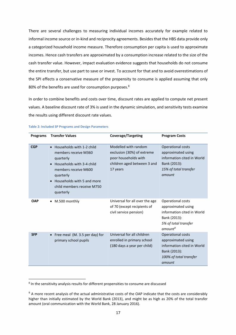
There are several challenges to measuring individual incomes accurately for example related to

informal income source or in-kind and reciprocity agreements. Besides that the HBS data provide only

a categorized household income measure. Therefore consumption per capita is used to approximate

incomes. Hence cash transfers are approximated by a consumption increase related to the size of the

cash transfer value. However, impact evaluation evidence suggests that households do not consume

the entire transfer, but use part to save or invest. To account for that and to avoid overestimations of

the SPI effects a conservative measure of the propensity to consume is applied assuming that only

80% of the benefits are used for consumption purposes.8

In order to combine benefits and costs over time, discount rates are applied to compute net present

values. A baseline discount rate of 3% is used in the dynamic simulation, and sensitivity tests examine

the results using different discount rate values.

Table 2: Included SP Programs and Design Parameters

Programs Transfer Values Coverage/Targeting Program Costs

CGP Households with 1-2 child

members receive M360

quarterly

Households with 3-4 child

members receive M600

quarterly

Households with 5 and more

child members receive M750

quarterly

Modelled with random

exclusion (30%) of extreme

poor households with

children aged between 3 and

17 years

Operational costs

approximated using

information cited in World

Bank (2013):

15% of total transfer

amount

OAP M.500 monthly Universal for all over the age

of 70 (except recipients of

civil service pension)

Operational costs

approximated using

information cited in World

Bank (2013):

5% of total transfer

amount9

SFP Free meal (M. 3.5 per day) for

primary school pupils

Universal for all children

enrolled in primary school

(180 days a year per child)

Operational costs

approximated using

information cited in World

Bank (2013):

100% of total transfer

amount

8 In the sensitivity analysis results for different propensities to consume are discussed

9 A more recent analysis of the actual administrative costs of the OAP indicate that the costs are considerably

higher than initially estimated by the World Bank (2013), and might be as high as 20% of the total transfer amount (oral communication with the World Bank, 28 January 2016).

18

To test for complementarities of combined SP instruments, the simulations will first analyze the

individual RoR of CGP, OAP and SFP. In a second step the CGP and OAP programs will be analyzed as

a combined package to test the integrated effect of the programs.

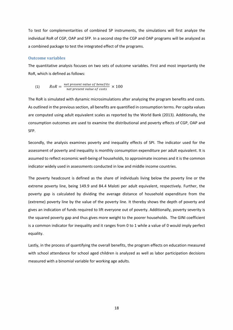
Outcome variables

The quantitative analysis focuses on two sets of outcome variables. First and most importantly the

RoR, which is defined as follows:

(1) 𝑅𝑜𝑅 = 𝑛𝑒𝑡 𝑝𝑟𝑒𝑠𝑒𝑛𝑡 𝑣𝑎𝑙𝑢𝑒 𝑜𝑓 𝑏𝑒𝑛𝑒𝑓𝑖𝑡𝑠

𝑛𝑒𝑡 𝑝𝑟𝑒𝑠𝑒𝑛𝑡 𝑣𝑎𝑙𝑢𝑒 𝑜𝑓 𝑐𝑜𝑠𝑡𝑠 × 100

The RoR is simulated with dynamic microsimulations after analyzing the program benefits and costs.

As outlined in the previous section, all benefits are quantified in consumption terms. Per capita values

are computed using adult equivalent scales as reported by the World Bank (2013). Additionally, the

consumption outcomes are used to examine the distributional and poverty effects of CGP, OAP and

SFP.

Secondly, the analysis examines poverty and inequality effects of SPI. The indicator used for the

assessment of poverty and inequality is monthly consumption expenditure per adult equivalent. It is

assumed to reflect economic well-being of households, to approximate incomes and it is the common

indicator widely used in assessments conducted in low and middle income countries.

The poverty headcount is defined as the share of individuals living below the poverty line or the

extreme poverty line, being 149.9 and 84.4 Maloti per adult equivalent, respectively. Further, the

poverty gap is calculated by dividing the average distance of household expenditure from the

(extreme) poverty line by the value of the poverty line. It thereby shows the depth of poverty and

gives an indication of funds required to lift everyone out of poverty. Additionally, poverty severity is

the squared poverty gap and thus gives more weight to the poorer households. The GINI coefficient

is a common indicator for inequality and it ranges from 0 to 1 while a value of 0 would imply perfect

equality.

Lastly, in the process of quantifying the overall benefits, the program effects on education measured

with school attendance for school aged children is analyzed as well as labor participation decisions

measured with a binomial variable for working age adults.

19

5. Data and Methodology

Data

In order to estimate rates of return of social protection interventions, micro-level data are required

for the analysis. At the core of the data requirements is a comprehensive household income and/or

consumption module, which allows determining household welfare and which is suitable for

quantifying the effects of social protection. Furthermore, the data should be nationally representative

and provide information on all possible links between social protection and household welfare

dimensions, such as education, health, labor, or livelihoods, in order to quantify the expected benefits

of social protection interventions. This means that the comprehensiveness and robustness of the

analysis is essentially determined by data availability.

The availability of household survey data in Lesotho is limited. During the inception mission, the team

together with UNICEF and the Bureau of Statistics identified all nationally representative household

data sets that could meet the data requirements of the analysis and decided to use the Household

Budget Survey (HBS). The Bureau of Statistics is in charge of the HBS. The survey is administered in

four waves over one year in order to capture seasonal variations. Over the last 20 years, the HBS has

been implemented three times with the latest round conducted in 2010/2011. The survey collects

data on households and individuals focusing on indicators relevant for the analysis of poverty and

welfare as well as education and labor statistics. The HBS is representative at the national and district

level, covering each of the ten districts and distinguishing between urban and rural regions.

Initially, it was decided to use the HBS 2010/11 data given that it is the most recent dataset which

contains detailed information on household consumption and hence meets the essential

requirements for the statistical estimations. However, as indicated by the World Bank, the

consumption data collected in 2010/2011 have to be treated with caution (World Bank, 2015b). The

2010/11 HBS differs from the previous round collected in 2002/03. In 2010/11, the HBS was integrated

with the Continuous Multipurpose Survey (CMS) that was launched in 2009 and implemented

annually. In this process, the survey instruments changed considerably. For example, the diary, which

is used to collect detailed information on household expenditures on food, drinks and other

consumables, covered only a one-week period compared to four weeks in the 2002/03 round.

According to the World Bank (2015b), the 2010/11 data collection suffered from high attrition after

the first quarter. Only 35 percent of the households could be revisited in the subsequent three

quarters. Moreover, the change in survey instruments resulted in almost half of the households in the

first quarter not reporting consumption of staple foods (Allwine et al. (2013) in: World Bank, 2015b).

20

Given that a reliable consumption aggregate is the key indicator for the analysis of social protection

benefits, the team decided to use the 2002/03 HBS data. The response rate in 2002/2003 was 87.1

percent. With households completing a consumption diary and receiving visits for face to face

interviews over a period of one month per survey wave, the survey provides comprehensive

information on consumption expenditure for specific goods, both in cash and in kind. It is therefore

considered the most appropriate dataset for this report as it facilitates the analysis of consumption

patterns in combination with labor and education indicators. As the HBS only covers standard

demographic and consumption variables, the data set is not suitable for drawing linkages between SP

and health or agricultural effects.

Limitations

There are several challenges in terms of data availability and quantification problems that impede to

incorporate all possibly existing linkages of SP in the study. These limitations need to be born in mind

in the interpretation of results as they might lead to an underestimation of the RoR. However, the

study can only descriptively point out potential missing links based on theory and findings of other

studies. Therefore it has to be noted that the following aspects cannot be incorporated in the

simulation models:

Due to the lack of appropriate data in the HBS, the link between SP and agricultural outcomes

such as investments in productive capital cannot be taken into account. The 2002/03 HBS does

not contain information on cultivation of land or livestock. Enterprise and detailed livelihood

information are not sufficiently covered in the HBS data to account for local multiplier effects in

the simulations.10

Information on health, disability or orphan status is also not available. The data therefore do not

permit a simulation of the OVC bursary benefit or the Public Assistance scheme. Furthermore, the

survey does not link households to their respective category in the NISSA system, which implies

that in the simulation of the CGP program eligibility is based on extreme poverty status rather

than belonging to NISSA category 1 or 2.

For the demographic projections, which are part of the dynamic simulation model, the study uses age-

specific mortality rates for Lesotho derived from the Global Health Observatory Data (WHO). Fertility

rates are based on projections of the BOS (2010).

10 This also applies to the 2010/11 HBS.

21

Methodology

Following the reduced study framework the simulation model aggregates direct and behavioral

benefits and compares them to the costs. To start we present a static model in which we simulate the

immediate direct effects of CGP, OAP and SFP effect on inequality and poverty outcomes.

Before testing the dynamic effects of the programs over several periods, the behavioral effects need

to be quantified. Thus the causal effect of a consumption increase on human capital needs to be

separated from the reversed causal effect of human capital on the level of consumption. Therefore

the indirect pathways are estimated stepwise: in the first step the effect of cash transfers on education

and labor participation is estimated. In the second step the returns to changes in educational decisions

are quantified estimating the effect of the highest educational attainment on household consumption

levels. The results describe the monetary returns to social transfers through the behavioral changes

on educational decisions. The methodological details and estimation formulas are presented in the

next section.

Subsequently, dynamic simulations estimate the RoR of CGP, OAP and SFP in each year from 1 to 15.

In each period the model tests whether the program eligibility criteria are met according to the

program targeting. If so, transfer values of the SP programs are assigned to the beneficiary. Moreover,

the model assigns the behavioral benefits in each period to past and current participants as estimated

in steps 1 and 2. The RoR are calculated for each period by comparing the monetarized benefits of SP

to the costs of SP. All values are discounted to net present values. The costs and benefits are computed

as the difference in a scenario with SP compared to a scenario without SP. That means, that in the

study the hypothetical case of SP investments is compared to a case without SP to test how

investments in SP would generate monetary returns.

A demographic module accounts for population ageing, mortality rates, and new borns according to

population projections by the WHO. Therefore, individuals age (stepwise) 15 years from the first to

the last period. Furthermore, the demographic model includes probabilities of newborns for women

in childbearing age and the probability of death per age group.

Consumption plays the essential role in the analysis of the RoR and poverty outcomes of SPI. It is used

to quantify the returns to education and fills the role of a common basis for the aggregation of

monetary benefits. Thus, before presenting the quantitative results, the consumption levels and the

baseline scenario without SPI is described. Table 3 displays the consumption level per capita according

to the HBS 2002 data. The average consumption level per adult equivalent was around 228 Maloti per

month with a large discrepancy between urban and rural consumption. The disaggregated values

show that urban consumption levels are about two thirds higher than rural consumption levels. This

22

is also reflected in significantly larger prevalence of poverty and especially extreme poverty levels in

rural areas. Based on our calculations, the data indicate that in 2002/2003 around 52% of the

population fall below the consumption poverty line of 149.91 Maloti.11 The share of extremely poor is

nearly twice as high in rural areas compared to urban regions. The inequality levels, as measured with

the GINI coefficient, are persistently high with a GINI of 0.52 with only minor differences between

urban and rural areas.

Table 3 Average (monthly) Consumption, Poverty and Inequality in Lesotho

Total Rural Urban

Consumption per capita 227 M. 171 M. 290 M.

Absolute Poverty (headcount)12 52.2% 62.5% 40.4%

Extreme Poverty (headcount) 30.3% 38.7% 20.8%

Inequality (GINI) 0.52 0.50 0.50

Note: Own calculations based on HBS 2002.

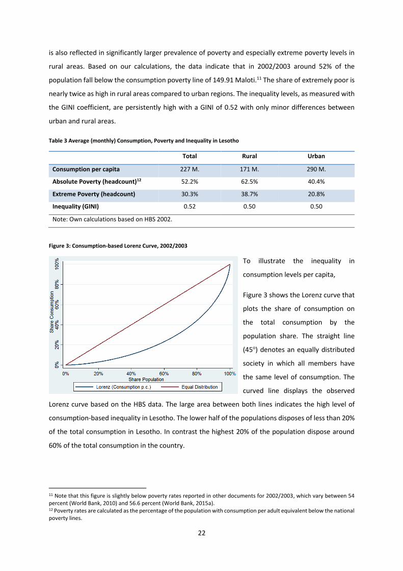
Figure 3: Consumption-based Lorenz Curve, 2002/2003

To illustrate the inequality in

consumption levels per capita,

Figure 3 shows the Lorenz curve that

plots the share of consumption on

the total consumption by the

population share. The straight line

(45○) denotes an equally distributed

society in which all members have

the same level of consumption. The

curved line displays the observed

Lorenz curve based on the HBS data. The large area between both lines indicates the high level of

consumption-based inequality in Lesotho. The lower half of the populations disposes of less than 20%

of the total consumption in Lesotho. In contrast the highest 20% of the population dispose around

60% of the total consumption in the country.

11 Note that this figure is slightly below poverty rates reported in other documents for 2002/2003, which vary between 54 percent (World Bank, 2010) and 56.6 percent (World Bank, 2015a). 12 Poverty rates are calculated as the percentage of the population with consumption per adult equivalent below the national poverty lines.

23

6. Analysis and Results

Static simulation

To test how SPI affects distributional and poverty outcomes in Lesotho, the results of static

microsimulations at the individual level are presented in this section. Which distributional and poverty

effects can we expect from CGP, OAP and SFP and a combined set of SPI?

Based on the HBS data and the SPI design assumptions (see Table 2), the direct distributional (𝐺) and

poverty (𝑃0) effects of the programs are simulated. Note that in this section the behavioral responses

are not (yet) included. To quantify the benefits (𝐵), the baseline without SPI is compared to a scenario

with SPI, assigning the difference in both scenarios to the direct program effects.

Equation (1) 𝐵𝑃 = [(𝑃1 − 𝑃0)/𝑃0] × 100

Equation (2) 𝐵𝐺 = [(𝐺1 − 𝐺0)/𝐺0] × 100

The static simulation is applied to CGP, OAP and SFP separately and the combined package of CGP and

OAP in combination. Table 4 displays the transfer values, costs and number of beneficiaries according

to the static simulation. Total annual transfer values are largest for the OAP, followed by the CGP and

the SFP. In terms of percentage of GDP, it matters greatly what year is used for the comparison.

Expressed as a percentage of GDP in 2003, the OAP accounts for 4.8%, and the CGP and SFP for 1.4%

and 1.2% respectively. Taking 2013 as benchmark, the share of GDP that would have to be allocated

to the three programs has decreased significantly. This is not surprising given that GDP in 2013 was

almost three times the value of 2003 in nominal terms. The results also differ compared to Table 1,

which contained actual data with respect to the number of beneficiaries and costs incurred, while

Table 4 shows the simulated values based on the HBS data 2002/2003. The considerably lower value

for OAP is mainly due to the lower number of persons aged 70 and older in 2002/2003. A similar

observation can be made for the SFP. The data below indicate that much fewer children have been

attending primary school in 2002/2003 compared to the current situation. The difference in costs and

beneficiaries of the CGP is due to the nationwide coverage of the program in the simulation.

Table 5 displays the results of the static simulations on poverty and inequality outcomes. The figures

illustrate the percentage decrease in outcome variables compared to the baseline scenario without

SPI. The outcomes are simulated for CGP, OAP, SFP, and a scenario combining OAP and CGP. It has to

be noted that the static simulation only regards the immediate impact on the outcome variables

without considering any demographic or educational dynamics.

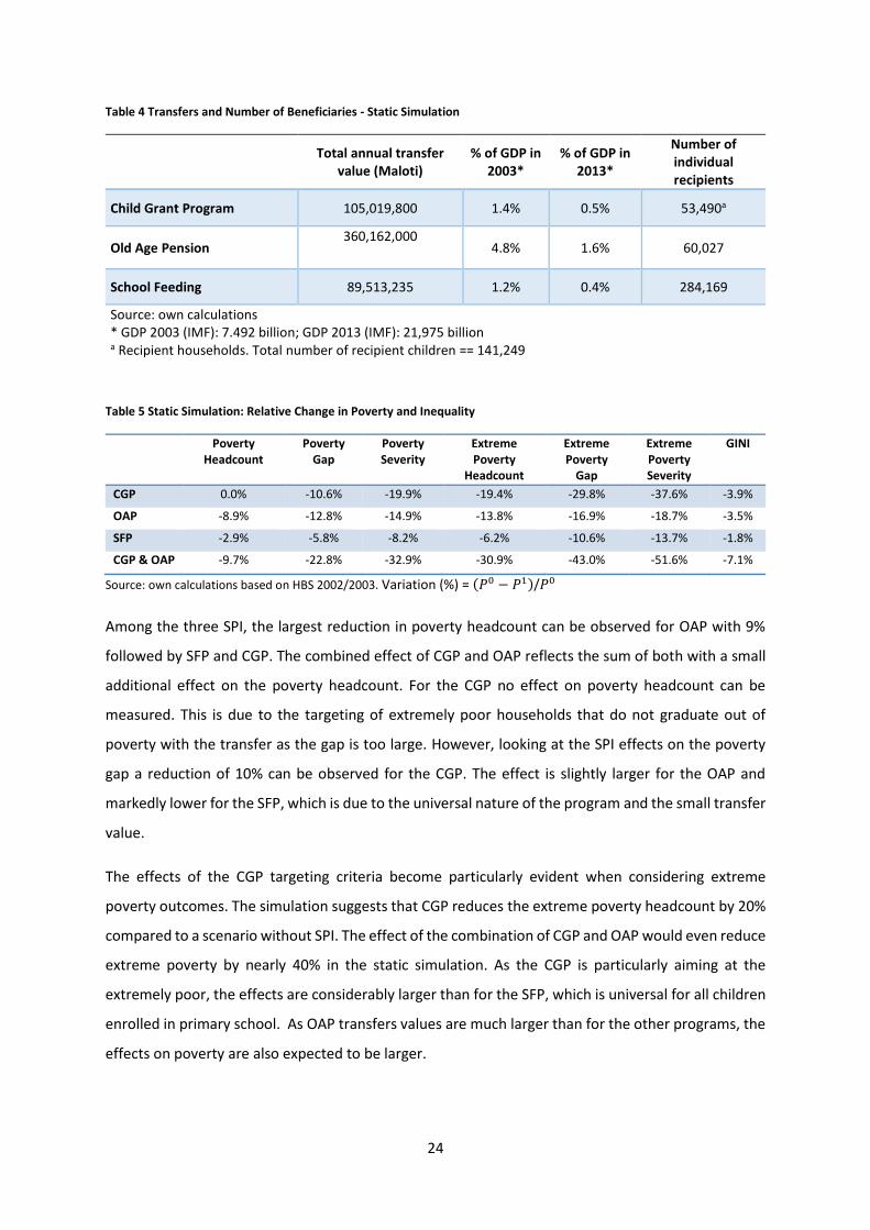
24

Table 4 Transfers and Number of Beneficiaries - Static Simulation

Total annual transfer

value (Maloti) % of GDP in

2003* % of GDP in

2013*

Number of individual recipients

Child Grant Program 105,019,800 1.4% 0.5% 53,490a

Old Age Pension 360,162,000

4.8% 1.6% 60,027

School Feeding 89,513,235 1.2% 0.4% 284,169

Source: own calculations * GDP 2003 (IMF): 7.492 billion; GDP 2013 (IMF): 21,975 billion a Recipient households. Total number of recipient children == 141,249

Table 5 Static Simulation: Relative Change in Poverty and Inequality

Poverty Headcount

Poverty Gap

Poverty Severity

Extreme Poverty

Headcount

Extreme Poverty

Gap

Extreme Poverty Severity

GINI

CGP 0.0% -10.6% -19.9% -19.4% -29.8% -37.6% -3.9%

OAP -8.9% -12.8% -14.9% -13.8% -16.9% -18.7% -3.5%

SFP -2.9% -5.8% -8.2% -6.2% -10.6% -13.7% -1.8%

CGP & OAP -9.7% -22.8% -32.9% -30.9% -43.0% -51.6% -7.1%

Source: own calculations based on HBS 2002/2003. Variation (%) = (𝑃0 − 𝑃1)/𝑃0

Among the three SPI, the largest reduction in poverty headcount can be observed for OAP with 9%

followed by SFP and CGP. The combined effect of CGP and OAP reflects the sum of both with a small

additional effect on the poverty headcount. For the CGP no effect on poverty headcount can be

measured. This is due to the targeting of extremely poor households that do not graduate out of

poverty with the transfer as the gap is too large. However, looking at the SPI effects on the poverty

gap a reduction of 10% can be observed for the CGP. The effect is slightly larger for the OAP and

markedly lower for the SFP, which is due to the universal nature of the program and the small transfer

value.

The effects of the CGP targeting criteria become particularly evident when considering extreme

poverty outcomes. The simulation suggests that CGP reduces the extreme poverty headcount by 20%

compared to a scenario without SPI. The effect of the combination of CGP and OAP would even reduce

extreme poverty by nearly 40% in the static simulation. As the CGP is particularly aiming at the

extremely poor, the effects are considerably larger than for the SFP, which is universal for all children

enrolled in primary school. As OAP transfers values are much larger than for the other programs, the

effects on poverty are also expected to be larger.

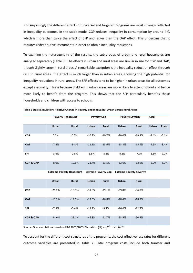
25

Not surprisingly the different effects of universal and targeted programs are most strongly reflected

in inequality outcomes. In the static model CGP reduces inequality in consumption by around 4%,

which is more than twice the effect of SFP and larger than the OAP effect. This underpins that it

requires redistributive instruments in order to obtain inequality reductions.

To examine the heterogeneity of the results, the sub-groups of urban and rural households are

analyzed separately (Table 6). The effects in urban and rural areas are similar in size for CGP and OAP,

though slightly larger in rural areas. A remarkable exception is the inequality reduction effect through

CGP in rural areas. The effect is much larger than in urban areas, showing the high potential for

inequality reductions in rural areas. The SFP effects tend to be higher in urban areas for all outcomes

except inequality. This is because children in urban areas are more likely to attend school and hence

more likely to benefit from the program. This shows that the SFP particularly benefits those

households and children with access to schools.

Table 6 Static Simulation: Relative Change in Poverty and Inequality, Urban versus Rural Areas

Poverty Headcount Poverty Gap Poverty Severity GINI

Urban Rural Urban Rural Urban Rural Urban Rural

CGP 0.0% 0.0% -10.3% -10.7% -20.0% -19.9% -2.4% -6.1%

OAP -7.4% -9.8% -11.1% -13.6% -13.8% -15.4% -2.6% -3.4%

SFP -3.6% -2.5% -6.8% -5.3% -9.5% -7.7% -1.6% -2.2%

CGP & OAP -8.0% -10.6% -21.4% -23.5% -32.6% -32.9% -5.0% -8.7%

Extreme Poverty Headcount Extreme Poverty Gap Extreme Poverty Severity

Urban Rural Urban Rural Urban Rural

CGP -21.2% -18.5% -31.8% -29.1% -39.8% -36.8%

OAP -13.2% -14.0% -17.0% -16.8% -18.4% -18.8%

SFP -7.8% -5.4% -12.7% -9.7% -16.4% -12.7%

CGP & OAP -34.6% -29.1% -46.3% -41.7% -53.5% -50.9%

Source: Own calculations based on HBS 2002/2003. Variation (%) = (𝑃0 − 𝑃1)/𝑃0

To account for the different cost structures of the programs, the cost effectiveness rates for different

outcome variables are presented in Table 7. Total program costs include both transfer and

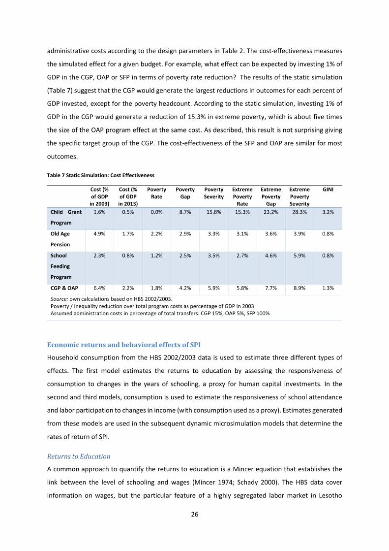
26

administrative costs according to the design parameters in Table 2. The cost-effectiveness measures

the simulated effect for a given budget. For example, what effect can be expected by investing 1% of

GDP in the CGP, OAP or SFP in terms of poverty rate reduction? The results of the static simulation

(Table 7) suggest that the CGP would generate the largest reductions in outcomes for each percent of

GDP invested, except for the poverty headcount. According to the static simulation, investing 1% of

GDP in the CGP would generate a reduction of 15.3% in extreme poverty, which is about five times

the size of the OAP program effect at the same cost. As described, this result is not surprising giving

the specific target group of the CGP. The cost-effectiveness of the SFP and OAP are similar for most

outcomes.

Table 7 Static Simulation: Cost Effectiveness

Cost (% of GDP

in 2003)

Cost (% of GDP

in 2013)

Poverty Rate

Poverty Gap

Poverty Severity

Extreme Poverty

Rate

Extreme Poverty

Gap

Extreme Poverty Severity

GINI

Child Grant

Program

1.6% 0.5% 0.0% 8.7% 15.8% 15.3% 23.2% 28.3% 3.2%

Old Age

Pension

4.9% 1.7% 2.2% 2.9% 3.3% 3.1% 3.6% 3.9% 0.8%

School

Feeding

Program

2.3% 0.8% 1.2% 2.5% 3.5% 2.7% 4.6% 5.9% 0.8%

CGP & OAP 6.4% 2.2% 1.8% 4.2% 5.9% 5.8% 7.7% 8.9% 1.3%

Source: own calculations based on HBS 2002/2003. Poverty / Inequality reduction over total program costs as percentage of GDP in 2003 Assumed administration costs in percentage of total transfers: CGP 15%, OAP 5%, SFP 100%

Economic returns and behavioral effects of SPI

Household consumption from the HBS 2002/2003 data is used to estimate three different types of

effects. The first model estimates the returns to education by assessing the responsiveness of

consumption to changes in the years of schooling, a proxy for human capital investments. In the

second and third models, consumption is used to estimate the responsiveness of school attendance

and labor participation to changes in income (with consumption used as a proxy). Estimates generated

from these models are used in the subsequent dynamic microsimulation models that determine the

rates of return of SPI.

Returns to Education

A common approach to quantify the returns to education is a Mincer equation that establishes the

link between the level of schooling and wages (Mincer 1974; Schady 2000). The HBS data cover

information on wages, but the particular feature of a highly segregated labor market in Lesotho

27

advocates for an alternative approach. Such an approach would need to account for the high levels of

informality in Lesotho. Alternatively, the returns to schooling at the household level are estimated by

using household consumption as a proxy for household disposable income. This allows for the direct

estimation of the effect of education on consumption which could also be interpreted as the monetary

returns to education and hence the returns of SPI through educational effects. The following model is

considered for estimation (equation 3):

Equation (3) ln(𝑐𝑜𝑛𝑠𝑢𝑚𝑝𝑡𝑖𝑜𝑛𝑖) = 𝛽 + 𝜌𝐸𝑖 + 𝜃𝑁𝑖 + 𝜋𝑖

where the logarithm of household consumption per adult equivalent i is used to approximate

income13, 𝐸𝑖 denotes the individual educational attainment measured by years of schooling for

individuals aged 18 to 69. 𝑁𝑖 refers to observable household characteristics such as age, sex, and

geographic control variables.

However, the main methodological problem with equation (3) is the two-way causal relationship of

consumption and education. On one side, increased household income (proxy is consumption) has a

positive effect on schooling either through reduced child labor or increased spending on education.

On the other side, education is an asset that boosts incomes. In order to correct for the potential bias

from reverse causality, an instrumental variable (IV) approach using a two-stage least squares model

is estimated. Education is instrumented with a variable measuring historical primary school

enrollment at district level. School enrollment data from 1979 to 2002 are used. Historical district level

school enrolment rates predict access to education which affects an individual’s educational

attainment, but they do not directly predict household consumption which justifies their use as an

instrumental variable. In the first stage the following model is estimated:

Equation (4) 𝐸𝑖 = 𝛾𝑍𝑖 + 𝜃𝑁𝑖 + 𝑒𝑖

Where 𝐸𝑖 refers to the educational attainment of individuals aged 18-69, which is instrumented using

𝑍𝑖 , historical district school enrollment rates.

Table 8 presents the results of the two-stage least squares (2SLS) model examining the returns to

education using household consumption per adult equivalent as a proxy for income. The results are

presented for the full sample and sub-populations of the poor, non-poor, urban and rural. The first

stage estimates an individual’s maximum level of education as a function of the instrumental variable

i.e. historical district school enrollment rates (equation 4). Using the minimum critical value of 10

13 Absolute household consumption values are normalized using the logarithm given the skewed distribution of household consumption and in order to account for outliers.

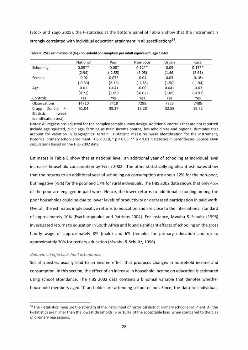
28

(Stock and Yogo 2005), the F-statistics at the bottom panel of Table 8 show that the instrument is

strongly correlated with individual education attainment in all specifications14.

Table 8. 2SLS estimation of (log) household consumption per adult equivalent, age 18-69

National Poor Non-poor Urban Rural

Schooling 0.09** -0.08* 0.12** 0.05 0.17** (2.94) (-2.55) (3.05) (1.46) (2.61) Female -0.02 0.07* -0.04 0.03 -0.18+ (-0.83) (2.12) (-1.38) (1.50) (-1.94) Age 0.01 0.04+ -0.00 0.04+ -0.03 (0.71) (1.89) (-0.02) (1.85) (-0.97) Controls Yes Yes Yes Yes Yes

Observations 14710 7418 7298 7225 7485 Cragg Donald F-Statistic (weak identification test)

51.04 38.27 15.28 32.58 19.72

Notes: All regressions adjusted for the complex sample survey design. Additional controls that are not reported include age squared, cubic age, farming as main income source, household size and regional dummies that account for variation in geographical terrain. F-statistic measures weak identification for the instrument, historical primary school enrolment. + p < 0.10, * p < 0.05, ** p < 0.01. t statistics in parentheses. Source: Own calculations based on the HBS 2002 data.

Estimates in Table 8 show that at national level, an additional year of schooling at individual level

increases household consumption by 9% in 2002. The other statistically significant estimates show

that the returns to an additional year of schooling on consumption are about 12% for the non-poor,

but negative (-8%) for the poor and 17% for rural individuals. The HBS 2002 data shows that only 45%

of the poor are engaged in paid work. Hence, the lower returns to additional schooling among the

poor households could be due to lower levels of productivity or decreased participation in paid work.

Overall, the estimates imply positive returns to education and are close to the international standard

of approximately 10% (Psacharopoulos and Patrinos 2004). For instance, Mwabu & Schultz (1996)

investigated returns to education in South Africa and found significant effects of schooling on the gross

hourly wage of approximately 8% (male) and 6% (female) for primary education and up to

approximately 30% for tertiary education (Mwabu & Schultz, 1996).

Behavioral effects: School attendance

Social transfers usually lead to an income effect that produces changes in household income and

consumption. In this section, the effect of an increase in household income on education is estimated

using school attendance. The HBS 2002 data contains a binomial variable that denotes whether

household members aged 10 and older are attending school or not. Since, the data for individuals

14 The F-statistics measure the strength of the instrument of historical district primary school enrollment. All the F-statistics are higher than the lowest thresholds (5 or 10%) of the acceptable bias when compared to the bias of ordinary regressions.

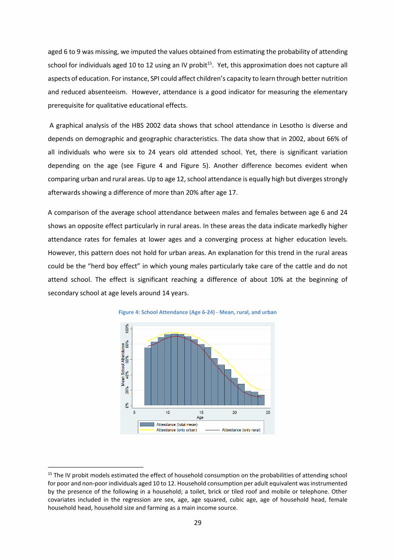
29

aged 6 to 9 was missing, we imputed the values obtained from estimating the probability of attending

school for individuals aged 10 to 12 using an IV probit15. Yet, this approximation does not capture all

aspects of education. For instance, SPI could affect children’s capacity to learn through better nutrition

and reduced absenteeism. However, attendance is a good indicator for measuring the elementary

prerequisite for qualitative educational effects.

A graphical analysis of the HBS 2002 data shows that school attendance in Lesotho is diverse and

depends on demographic and geographic characteristics. The data show that in 2002, about 66% of

all individuals who were six to 24 years old attended school. Yet, there is significant variation

depending on the age (see Figure 4 and Figure 5). Another difference becomes evident when

comparing urban and rural areas. Up to age 12, school attendance is equally high but diverges strongly

afterwards showing a difference of more than 20% after age 17.

A comparison of the average school attendance between males and females between age 6 and 24

shows an opposite effect particularly in rural areas. In these areas the data indicate markedly higher

attendance rates for females at lower ages and a converging process at higher education levels.

However, this pattern does not hold for urban areas. An explanation for this trend in the rural areas

could be the “herd boy effect” in which young males particularly take care of the cattle and do not

attend school. The effect is significant reaching a difference of about 10% at the beginning of

secondary school at age levels around 14 years.

Figure 4: School Attendance (Age 6-24) - Mean, rural, and urban

15 The IV probit models estimated the effect of household consumption on the probabilities of attending school for poor and non-poor individuals aged 10 to 12. Household consumption per adult equivalent was instrumented by the presence of the following in a household; a toilet, brick or tiled roof and mobile or telephone. Other covariates included in the regression are sex, age, age squared, cubic age, age of household head, female household head, household size and farming as a main income source.

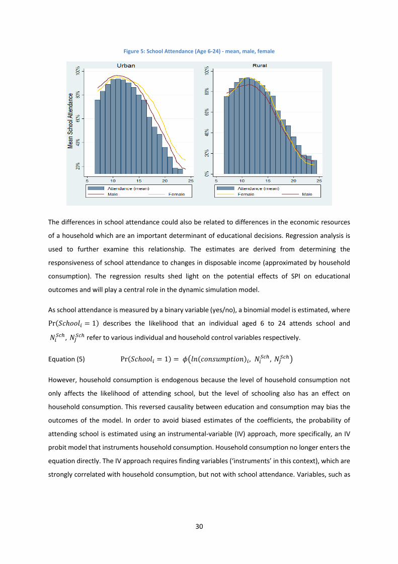
30

Figure 5: School Attendance (Age 6-24) - mean, male, female

The differences in school attendance could also be related to differences in the economic resources

of a household which are an important determinant of educational decisions. Regression analysis is

used to further examine this relationship. The estimates are derived from determining the

responsiveness of school attendance to changes in disposable income (approximated by household

consumption). The regression results shed light on the potential effects of SPI on educational

outcomes and will play a central role in the dynamic simulation model.

As school attendance is measured by a binary variable (yes/no), a binomial model is estimated, where

Pr(𝑆𝑐ℎ𝑜𝑜𝑙𝑖 = 1) describes the likelihood that an individual aged 6 to 24 attends school and

𝑁𝑖𝑆𝑐ℎ , 𝑁𝐽

𝑆𝑐ℎ refer to various individual and household control variables respectively.

Equation (5) Pr(𝑆𝑐ℎ𝑜𝑜𝑙𝑖 = 1) = 𝜙(𝑙𝑛(𝑐𝑜𝑛𝑠𝑢𝑚𝑝𝑡𝑖𝑜𝑛)𝑖, 𝑁𝑖𝑆𝑐ℎ , 𝑁𝐽

𝑆𝑐ℎ)

However, household consumption is endogenous because the level of household consumption not

only affects the likelihood of attending school, but the level of schooling also has an effect on

household consumption. This reversed causality between education and consumption may bias the

outcomes of the model. In order to avoid biased estimates of the coefficients, the probability of

attending school is estimated using an instrumental-variable (IV) approach, more specifically, an IV

probit model that instruments household consumption. Household consumption no longer enters the

equation directly. The IV approach requires finding variables (‘instruments’ in this context), which are

strongly correlated with household consumption, but not with school attendance. Variables, such as

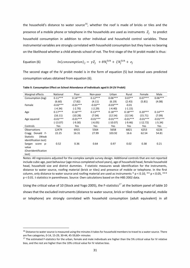
31

the household’s distance to water source16, whether the roof is made of bricks or tiles and the

presence of a mobile phone or telephone in the households are used as instruments 𝑍𝑗 to predict

household consumption in addition to other individual and household control variables. These

instrumental variables are strongly correlated with household consumption but they have no bearing

on the likelihood whether a child attends school of not. The first stage of the IV probit model is thus:

Equation (6) 𝑙𝑛(𝑐𝑜𝑛𝑠𝑢𝑚𝑝𝑡𝑖𝑜𝑛)𝑗 = 𝛾𝑍𝑗 + 𝜃𝑁𝑖𝑆𝑐ℎ + 𝜉𝑁𝑗

𝑆𝑐ℎ + 𝑒𝑗

The second stage of the IV probit model is in the form of equation (5) but instead uses predicted

consumption values obtained from equation (6).

Table 9. Consumption Effect on School Attendance of Individuals aged 6-24 (IV Probit)

Marginal effects National Poor Non-poor Urban Rural Female Male

Consumption (log) 0.11*** 0.14*** 0.12*** 0.06*** 0.07** 0.07*** 0.06*** (6.60) (7.82) (4.11) (6.19) (2.43) (5.81) (4.08) Female -0.02*** -0.01*** -0.02** -0.03*** -0.01 (-4.34) (-2.70) (-2.29) (-4.40) (-1.15) Age 0.17*** 0.16*** 0.13*** 0.18*** 0.18*** 0.20*** 0.14*** (16.11) (10.28) (7.04) (12.54) (12.54) (15.71) (7.09) Age squared -0.01*** -0.01*** -0.01*** -0.01*** -0.01*** -0.01*** -0.01*** (-13.07) (-9.30) (-6.05) (-10.07) (-9.46) (-12.72) (-5.34) Controls Yes Yes Yes Yes Yes Yes Yes

Observations 12479 6915 5564 5658 6821 6253 6226 Cragg Donald F- Statistic (Weak identification test)

22.25 16.31 27.99 103.92 16.6 62.54 54.81

Sargan score p-value (Overidentification test)

0.52 0.36 0.64 0.97 0.02 0.38 0.21

Notes: All regressions adjusted for the complex sample survey design. Additional controls that are not reported include cubic age, past behaviour (age minus completed school years), age of household head, female household head, household size and district dummies. F-statistic measures weak identification for the instruments, distance to water source, roofing material (brick or tiles) and presence of mobile or telephone. In the first column, only distance to water source and roofing material are used as instruments * p < 0.10, ** p < 0.05, *** p < 0.01. t statistics in parentheses. Source: Own calculations based on the HBS 2002 data.

Using the critical value of 10 (Stock and Yogo 2005), the F-statistics17 at the bottom panel of table 10

shows that the excluded instruments (distance to water source, brick or tiled roofing material, mobile

or telephone) are strongly correlated with household consumption (adult equivalent) in all

16 Distance to water source is measured using the minutes it takes for household members to travel to a water source. There

are five categories, 0-14, 15-29, 30-44, 45-59,60+ minutes 17 The estimated F-statistics for the urban, female and male individuals are higher than the 5% critical value for IV relative

bias, and the rest are higher than the 10% critical value for IV relative bias.

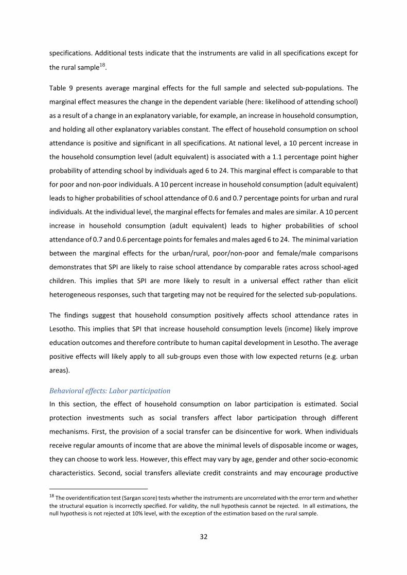
32

specifications. Additional tests indicate that the instruments are valid in all specifications except for

the rural sample18.

Table 9 presents average marginal effects for the full sample and selected sub-populations. The

marginal effect measures the change in the dependent variable (here: likelihood of attending school)

as a result of a change in an explanatory variable, for example, an increase in household consumption,

and holding all other explanatory variables constant. The effect of household consumption on school

attendance is positive and significant in all specifications. At national level, a 10 percent increase in

the household consumption level (adult equivalent) is associated with a 1.1 percentage point higher

probability of attending school by individuals aged 6 to 24. This marginal effect is comparable to that

for poor and non-poor individuals. A 10 percent increase in household consumption (adult equivalent)

leads to higher probabilities of school attendance of 0.6 and 0.7 percentage points for urban and rural

individuals. At the individual level, the marginal effects for females and males are similar. A 10 percent

increase in household consumption (adult equivalent) leads to higher probabilities of school

attendance of 0.7 and 0.6 percentage points for females and males aged 6 to 24. The minimal variation

between the marginal effects for the urban/rural, poor/non-poor and female/male comparisons

demonstrates that SPI are likely to raise school attendance by comparable rates across school-aged

children. This implies that SPI are more likely to result in a universal effect rather than elicit

heterogeneous responses, such that targeting may not be required for the selected sub-populations.

The findings suggest that household consumption positively affects school attendance rates in

Lesotho. This implies that SPI that increase household consumption levels (income) likely improve

education outcomes and therefore contribute to human capital development in Lesotho. The average

positive effects will likely apply to all sub-groups even those with low expected returns (e.g. urban

areas).

Behavioral effects: Labor participation

In this section, the effect of household consumption on labor participation is estimated. Social

protection investments such as social transfers affect labor participation through different

mechanisms. First, the provision of a social transfer can be disincentive for work. When individuals

receive regular amounts of income that are above the minimal levels of disposable income or wages,

they can choose to work less. However, this effect may vary by age, gender and other socio-economic

characteristics. Second, social transfers alleviate credit constraints and may encourage productive

18 The overidentification test (Sargan score) tests whether the instruments are uncorrelated with the error term and whether

the structural equation is incorrectly specified. For validity, the null hypothesis cannot be rejected. In all estimations, the null hypothesis is not rejected at 10% level, with the exception of the estimation based on the rural sample.

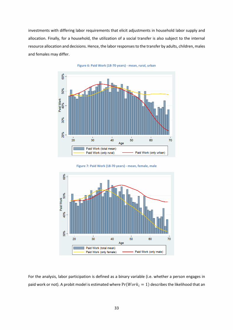
33

investments with differing labor requirements that elicit adjustments in household labor supply and

allocation. Finally, for a household, the utilization of a social transfer is also subject to the internal

resource allocation and decisions. Hence, the labor responses to the transfer by adults, children, males

and females may differ.

Figure 6: Paid Work (18-70 years) - mean, rural, urban

Figure 7: Paid Work (18-70 years) - mean, female, male

For the analysis, labor participation is defined as a binary variable (i.e. whether a person engages in

paid work or not). A probit model is estimated where Pr(𝑊𝑜𝑟𝑘𝑖 = 1) describes the likelihood that an

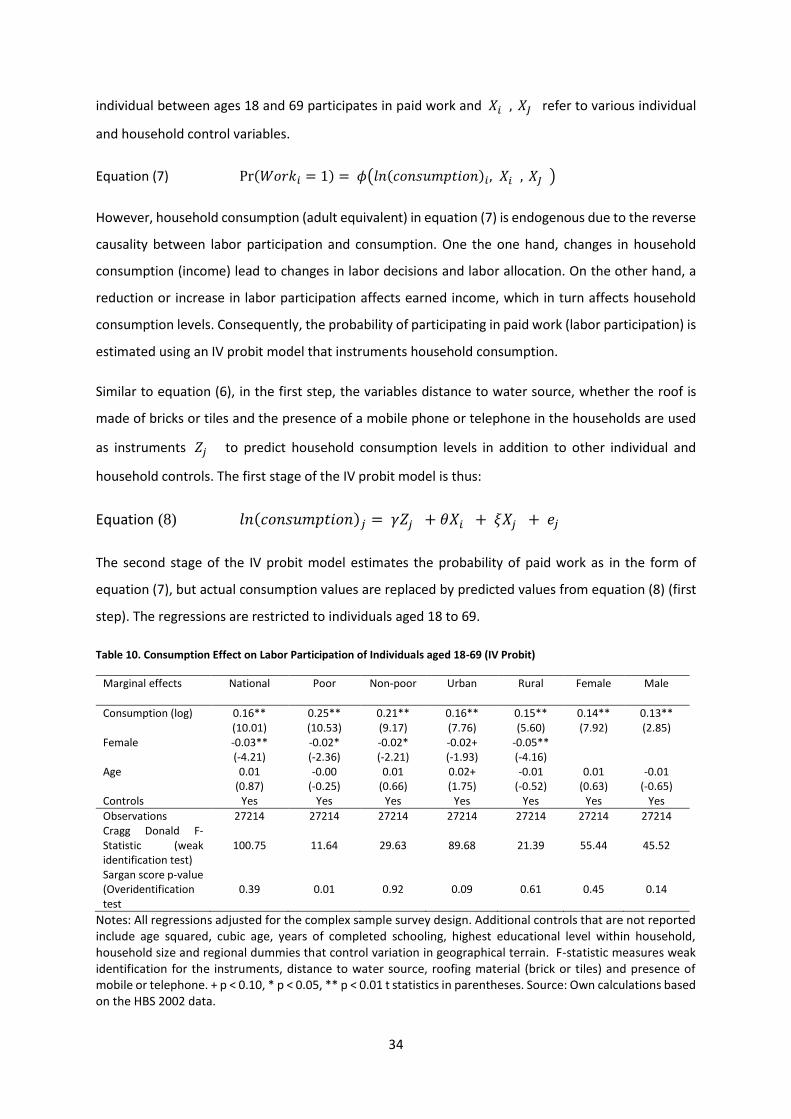
34

individual between ages 18 and 69 participates in paid work and 𝑋𝑖 , 𝑋𝐽 refer to various individual

and household control variables.

Equation (7) Pr(𝑊𝑜𝑟𝑘𝑖 = 1) = 𝜙(𝑙𝑛(𝑐𝑜𝑛𝑠𝑢𝑚𝑝𝑡𝑖𝑜𝑛)𝑖, 𝑋𝑖 , 𝑋𝐽 )

However, household consumption (adult equivalent) in equation (7) is endogenous due to the reverse

causality between labor participation and consumption. One the one hand, changes in household

consumption (income) lead to changes in labor decisions and labor allocation. On the other hand, a

reduction or increase in labor participation affects earned income, which in turn affects household

consumption levels. Consequently, the probability of participating in paid work (labor participation) is

estimated using an IV probit model that instruments household consumption.

Similar to equation (6), in the first step, the variables distance to water source, whether the roof is

made of bricks or tiles and the presence of a mobile phone or telephone in the households are used

as instruments 𝑍𝑗 to predict household consumption levels in addition to other individual and

household controls. The first stage of the IV probit model is thus:

Equation (8) 𝑙𝑛(𝑐𝑜𝑛𝑠𝑢𝑚𝑝𝑡𝑖𝑜𝑛)𝑗 = 𝛾𝑍𝑗 + 𝜃𝑋𝑖 + 𝜉𝑋𝑗 + 𝑒𝑗

The second stage of the IV probit model estimates the probability of paid work as in the form of

equation (7), but actual consumption values are replaced by predicted values from equation (8) (first

step). The regressions are restricted to individuals aged 18 to 69.

Table 10. Consumption Effect on Labor Participation of Individuals aged 18-69 (IV Probit)

Marginal effects National Poor Non-poor Urban Rural Female Male

Consumption (log) 0.16** 0.25** 0.21** 0.16** 0.15** 0.14** 0.13** (10.01) (10.53) (9.17) (7.76) (5.60) (7.92) (2.85) Female -0.03** -0.02* -0.02* -0.02+ -0.05** (-4.21) (-2.36) (-2.21) (-1.93) (-4.16) Age 0.01 -0.00 0.01 0.02+ -0.01 0.01 -0.01 (0.87) (-0.25) (0.66) (1.75) (-0.52) (0.63) (-0.65) Controls Yes Yes Yes Yes Yes Yes Yes

Observations 27214 27214 27214 27214 27214 27214 27214 Cragg Donald F- Statistic (weak identification test)

100.75

11.64

29.63

89.68

21.39

55.44

45.52

Sargan score p-value (Overidentification test

0.39

0.01

0.92

0.09

0.61

0.45

0.14

Notes: All regressions adjusted for the complex sample survey design. Additional controls that are not reported include age squared, cubic age, years of completed schooling, highest educational level within household, household size and regional dummies that control variation in geographical terrain. F-statistic measures weak identification for the instruments, distance to water source, roofing material (brick or tiles) and presence of mobile or telephone. + p < 0.10, * p < 0.05, ** p < 0.01 t statistics in parentheses. Source: Own calculations based on the HBS 2002 data.

35

Using the critical value of 10 (Stock and Yogo 2005), the F-statistics19 show that the excluded

instruments (distance to water source, brick or tiled roofing material, mobile or telephone) are

strongly correlated with household consumption (adult equivalent) in all specifications. Additional

tests indicate that the instruments are valid in all specifications except for poor individuals20.

Table 10 presents average marginal effects for labor participation for the full sample and selected sub-

populations. The results show that household consumption has a positive effect on labor participation

in all estimations. At national level, a 10 percent increase in the household consumption level (per

adult equivalent) is associated with a 1.6 percentage point increased probability of labor participation

by individuals aged 18 to 69. This marginal effect is comparable to that for urban and rural individuals.

A 10 percent increase in household consumption (adult equivalent) leads to higher probabilities of

labor participation of 2.5 and 2.1 percentage points for poor and no-poor individuals. At the individual

level, the marginal effects for females and males are similar. Similar to the findings on the probability

of school attendance, there is minimal variation in the average positive effects when the different sub-

populations are compared. Overall, the findings suggest that SPI that increase household consumption

levels (income) potentially raise participation in the labor markets in Lesotho.

Dynamic Simulation

The static simulation model showed the direct effects of SPI from the baseline year to the next. In this

section dynamic simulation model are applied to examine the effects over time including the

behavioral effects through increased school attendance and higher school attainments. Thus, the SPI

effects are simulated over a 15 years’ time range. The effects are simulated as if the programs were

implemented on the national level using nationally representative survey weights. The aim of the

dynamic simulation is to analyze the changes over time regarding human capital developments and

consumption. Therefore the dynamic model incorporates the behavioral responses as estimated in

equation 4 and 6. In order to refine the simulation the effect of consumption on school attendance

(equation 4) is simulated for poor and non-poor individuals separately. Thereby the much larger effect

of an additional Maloti for a poor household as compared to richer households regarding school

attendance is included in the simulations.

19 The estimated F-statistics are higher than the 5% critical value for IV relative bias in all cases except for poor individuals,

in which the F-statistic is higher than the 10% critical value for IV relative bias. 20 The overidentification test (Sargan score) tests whether the instruments are uncorrelated with the error term. For validity,

the null hypothesis cannot be rejected. In all estimations, except for those based on poor and urban individuals, the null hypothesis is not rejected at 10% level. The null hypothesis cannot be rejected at the 5% for estimations on urban individuals.

36

The model accounts for demographic changes during the 15-year simulation period regarding for

ageing, death, and newborns. The demographic module uses mortality rate projections by age and sex

to probabilistically determine deaths in each period. In the same way, yearly fertility rate projections

account for newborns of women in childbearing age (15-49) in each period. This demographic module

ensures that individuals change eligibility along the 15 years study framework. For example,

individuals that turn 70 during the simulation period become eligible for the OAP. On the other side,

households with children above 17 will no longer be eligible for the CGP.

Within the simulation model, population size increases at an average annual rate of 0.59% resulting

in an overall increase of 8.59% from 1.8 million in 2002 to 2.0 million in 2016. The resulting population

size in 2016 (1,949,196.82) is very close to a figure forecast by the IMF, based on the population census

in 2006 (1,920 million). The slow population growth reflects recent developments in Lesotho of

decreasing fertility rates and raising mortality rates. Figure 13 in the Annex summarizes the population

development according to the simulation model.

School attendance and educational attainment are used to predict the behavioral returns to SPI.

Therefore, the educational outcomes that can be expected with higher consumption levels due to the

SPI transfers is compared to the expected education outcomes without the transfers. In that regard

the behavioral benefits can be formulated as follows:

Equation (9) 𝐵𝑡=𝑇 = (𝐸𝑡=𝑇𝑆𝑃𝐼,1 − 𝐸𝑡=0

𝑆𝑃𝐼,0) − (𝐸𝑡=𝑇𝑆𝑃𝐼,0 − 𝐸𝑡=0

𝑆𝑃𝐼,0) = 𝐸𝑡=𝑇𝑆𝑃𝐼,1 − 𝐸𝑡=𝑇

𝑆𝑃𝐼,0

Where 𝐸𝑡=𝑇𝑆𝑃𝐼,1 refers to the expected consumption including the behavioral responses and 𝐸𝑡=𝑇

𝑆𝑃𝐼,0 to

the expected consumption in the absence of SPI transfers.

The consumption level is calibrated using the HBS 2002/2003 data. Based on the eligibility criteria of

the SPI, the transfers are assigned to individuals. Within households the benefits of SPI are equally

distributed among its members according to the adult equivalent weights. That means that individual

grants are shared with household members according to their respective weight within the household.

21

The simulation procedure remains the same in each period as outlined in Table 11: in the baseline

period consumption is determined by the HBS data. Assigned beneficiaries of the SPI receive the

benefits, which increases their consumption levels by the amount of the transfer values times the

propensity to consume (80%). Based on their new consumption level the likelihood of school age

21 Existing evidence advocates against the alternative assumption that pensions are not shared within households (e.g. Woolard & Klasen, 2005)

37

children to attend school is predicted (based on equation 4). Following this, the educational

attainment is updated probabilistically depending on whether children (age 6-24) attended school.

The behavioral benefits of SPI are computed as the difference of predicted consumption with and

without SPI as a function of the educational attainment as shown in equation 6. The new consumption

levels are calculated as the sum of the previous consumption level plus the direct effect (transfers)

and the behavioral benefit. The difference in consumption in a scenario with SPI and the baseline

without SPI reflects the overall benefits of the programs.

At the end of each period, the demographic changes are realized. In the next period households need

to qualify again for the SPI transfer and only the behavioral benefits are carried over to the next

period’s consumption. This procedure is automatically performed for 15 periods. Table 11 outlines the

simulation steps per period.

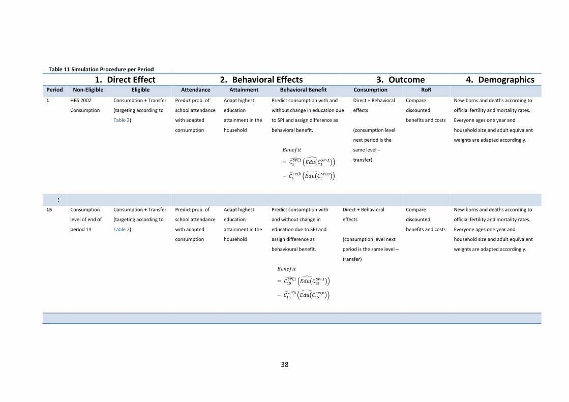
38

Table 11 Simulation Procedure per Period

1. Direct Effect 2. Behavioral Effects 3. Outcome 4. Demographics Period Non-Eligible Eligible Attendance Attainment Behavioral Benefit Consumption RoR

1 HBS 2002

Consumption

Consumption + Transfer

(targeting according to

Table 2)

Predict prob. of

school attendance

with adapted

consumption

Adapt highest

education

attainment in the

household

Predict consumption with and

without change in education due

to SPI and assign difference as

behavioral benefit.

𝐵𝑒𝑛𝑒𝑓𝑖𝑡

= 𝐶1𝑆𝑃𝑖,1̂ (𝐸𝑑𝑢(𝐶1

𝑆𝑃𝑖,1))̂

− 𝐶1𝑆𝑃𝑖,0̂ (𝐸𝑑𝑢(𝐶1

𝑆𝑃𝑖,0))̂

Direct + Behavioral

effects

(consumption level

next period is the

same level –

transfer)

Compare

discounted

benefits and costs

New-borns and deaths according to

official fertility and mortality rates.

Everyone ages one year and

household size and adult equivalent

weights are adapted accordingly.

...

15 Consumption

level of end of

period 14

Consumption + Transfer

(targeting according to

Table 2)

Predict prob. of

school attendance

with adapted

consumption

Adapt highest

education

attainment in the

household

Predict consumption with

and without change in

education due to SPI and

assign difference as

behavioural benefit.

𝐵𝑒𝑛𝑒𝑓𝑖𝑡

= 𝐶15𝑆𝑃𝑖,1̂ (𝐸𝑑𝑢(𝐶15

𝑆𝑃𝑖,1))̂

− 𝐶15𝑆𝑃𝑖,0̂ (𝐸𝑑𝑢(𝐶15

𝑆𝑃𝑖,0))̂

Direct + Behavioral

effects

(consumption level next

period is the same level –

transfer)

Compare

discounted

benefits and costs

New-borns and deaths according to

official fertility and mortality rates.

Everyone ages one year and

household size and adult equivalent

weights are adapted accordingly.

39

Dynamic Simulation Results

The dynamic simulation compares the outcomes of the programs to a scenario without SPI. Therefore,

the focus is not on predictions of outcome variables in future periods, but rather on the relative

development in outcomes compared to the control scenario.

Figure 8 presents the program effects on current school attendance relative to the baseline scenario

without SPI. The figure shows that all SPIs affect school attendance and educational attainments

positively. School attendance rates of individuals between 6 and 24 years increased strongest for the

CGP scenario and the combination of CGP and OAP. The CGP school attendance rate increased by 5%

in the first period, which grows up to an annual increase of more than 12% in period 15 compared to

the control scenario. As the SPI effects sum up over time later periods also include the returns to the

returns, which lead to an exponential growth in school attendance rates. As a consequence, after 15

periods the working-age adults dispose of a 2% higher school attainment in the CGP scenario as

compared to the control scenario.

The OAP effect on school attendance is markedly smaller ranging from 1.5% to around 10%. Despite

the larger transfer values of OAP the effect is lower as it is not targeted at children. The combination

of CGP and OAP further increases school attendance rates, however, adding only little to the CGP

effect.

The SFP effect on school attendance is smaller than the CGP effect and increases up to around 7% at

the end of the simulation period. Yet, the annual growth rates are smaller than for the other programs.

This is due to the SFP assignment to children that are already enrolled in school with thus little scope

to further increase attendance rates. However, it has to be noted that the potential effects of SFP on

aspects such as school performance or health cannot be regarded in the model.22 These effect

pathways could have important impacts on school attainments and lead to an underestimation of the

educational effects of SFP in the simulation model.

22 Data on school performance are not covered in the HBS 2002/2003.

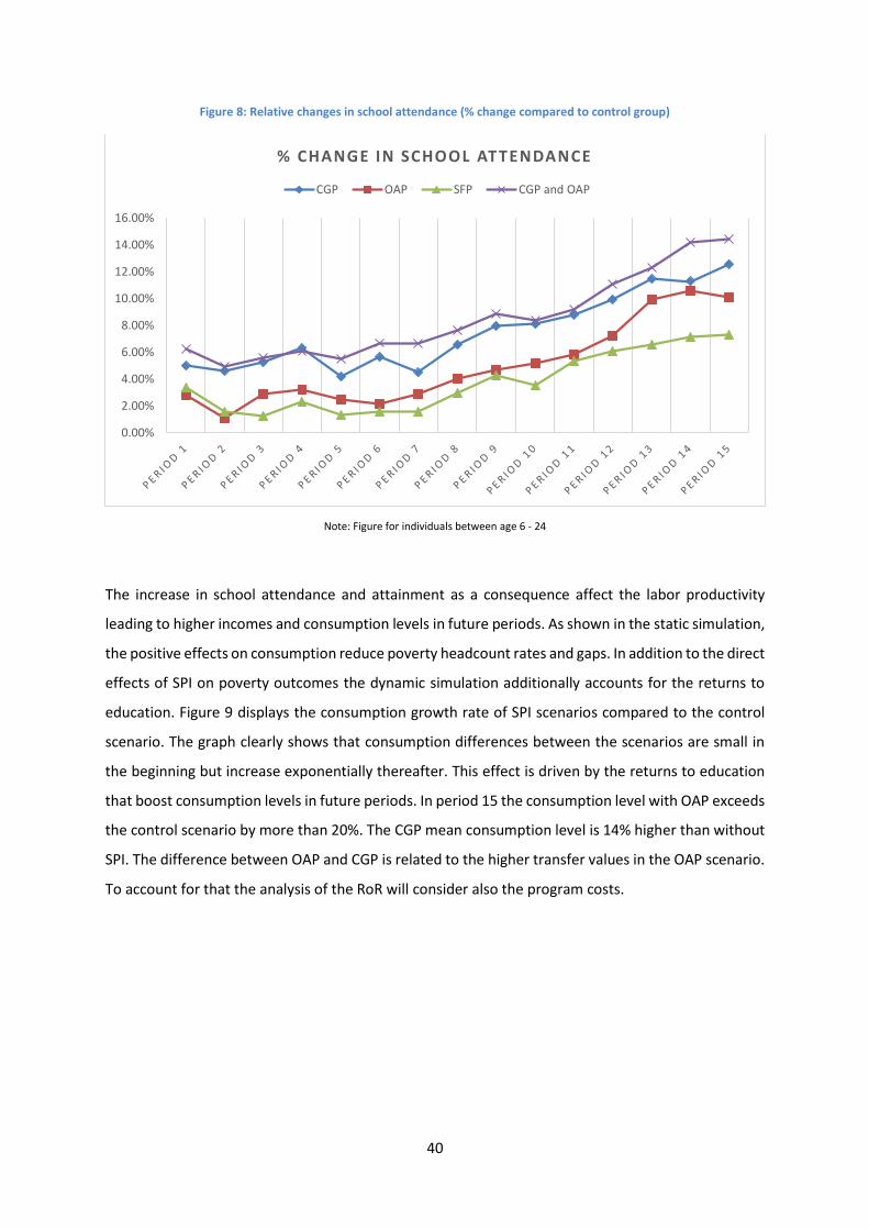
40

Figure 8: Relative changes in school attendance (% change compared to control group)

Note: Figure for individuals between age 6 - 24

The increase in school attendance and attainment as a consequence affect the labor productivity

leading to higher incomes and consumption levels in future periods. As shown in the static simulation,

the positive effects on consumption reduce poverty headcount rates and gaps. In addition to the direct

effects of SPI on poverty outcomes the dynamic simulation additionally accounts for the returns to

education. Figure 9 displays the consumption growth rate of SPI scenarios compared to the control

scenario. The graph clearly shows that consumption differences between the scenarios are small in

the beginning but increase exponentially thereafter. This effect is driven by the returns to education

that boost consumption levels in future periods. In period 15 the consumption level with OAP exceeds

the control scenario by more than 20%. The CGP mean consumption level is 14% higher than without

SPI. The difference between OAP and CGP is related to the higher transfer values in the OAP scenario.

To account for that the analysis of the RoR will consider also the program costs.

0.00%

2.00%

4.00%

6.00%

8.00%

10.00%

12.00%

14.00%

16.00%

% CHANGE IN SCHOOL AT TENDANCE

CGP OAP SFP CGP and OAP

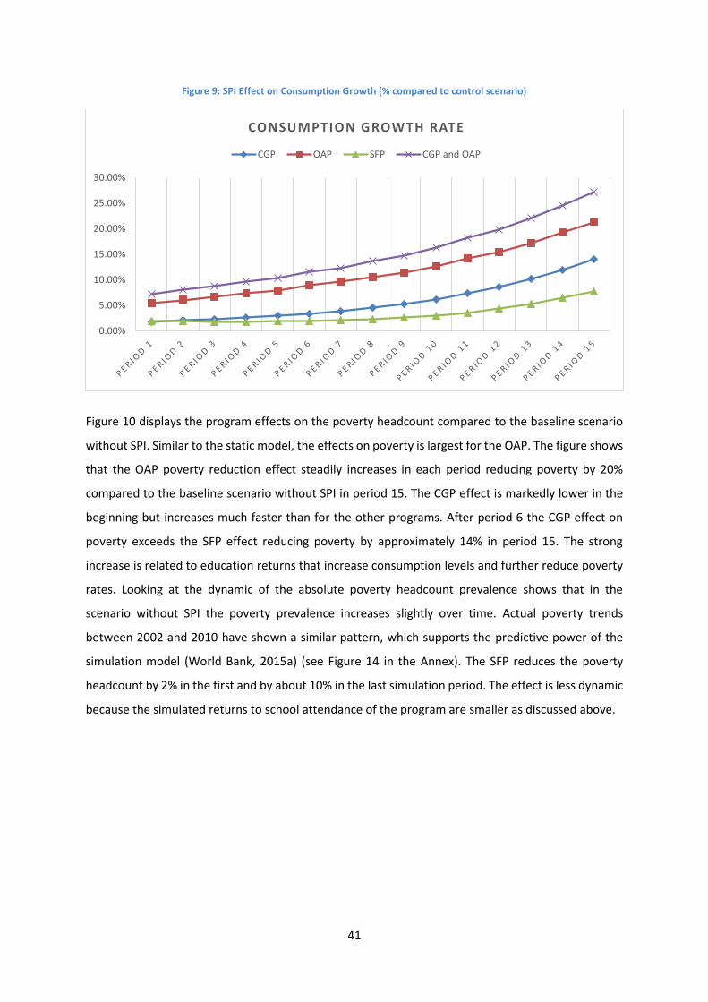
41

Figure 9: SPI Effect on Consumption Growth (% compared to control scenario)

Figure 10 displays the program effects on the poverty headcount compared to the baseline scenario

without SPI. Similar to the static model, the effects on poverty is largest for the OAP. The figure shows

that the OAP poverty reduction effect steadily increases in each period reducing poverty by 20%

compared to the baseline scenario without SPI in period 15. The CGP effect is markedly lower in the

beginning but increases much faster than for the other programs. After period 6 the CGP effect on

poverty exceeds the SFP effect reducing poverty by approximately 14% in period 15. The strong

increase is related to education returns that increase consumption levels and further reduce poverty

rates. Looking at the dynamic of the absolute poverty headcount prevalence shows that in the

scenario without SPI the poverty prevalence increases slightly over time. Actual poverty trends

between 2002 and 2010 have shown a similar pattern, which supports the predictive power of the

simulation model (World Bank, 2015a) (see Figure 14 in the Annex). The SFP reduces the poverty

headcount by 2% in the first and by about 10% in the last simulation period. The effect is less dynamic

because the simulated returns to school attendance of the program are smaller as discussed above.

0.00%

5.00%

10.00%

15.00%

20.00%

25.00%

30.00%

CONSUMPTION GROWTH RATE

CGP OAP SFP CGP and OAP

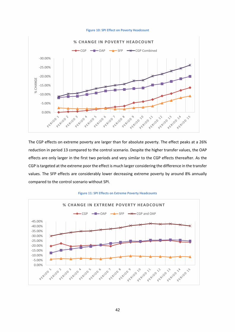
42

Figure 10: SPI Effect on Poverty Headcount

The CGP effects on extreme poverty are larger than for absolute poverty. The effect peaks at a 26%

reduction in period 13 compared to the control scenario. Despite the higher transfer values, the OAP

effects are only larger in the first two periods and very similar to the CGP effects thereafter. As the

CGP is targeted at the extreme poor the effect is much larger considering the difference in the transfer

values. The SFP effects are considerably lower decreasing extreme poverty by around 8% annually

compared to the control scenario without SPI.

Figure 11: SPI Effects on Extreme Poverty Headcounts

-30.00%

-25.00%

-20.00%

-15.00%

-10.00%

-5.00%

0.00%

% C

HA

NG

E

% CHANGE IN POVERTY HEADCOUNT

CGP OAP SFP CGP Combined

-45.00%

-40.00%

-35.00%

-30.00%

-25.00%

-20.00%

-15.00%

-10.00%

-5.00%

0.00%

% CHAN GE IN EXTREME POVERTY HEADCOUN T

CGP OAP SFP CGP and OAP

43

Table 12 summarizes all simulated outcomes for periods 5, 10, and 15. The effects of CGP and OAP on

consumption inequality measured with the GINI are similar in size. Both programs decrease inequality

by about 8% in period 15. The combination of both programs results in a decrease of 12% in inequality.

The SFP effects are smaller leading to a 3% decrease at the end of the simulation period.

Table 12 Dynamic benefits in periods 5, 10 and 15

Period 5 Period 10 Period 15

CGP Years in school 0.1% 0.9% 2.0%

Average household consumption growth rate per year 3.0% 6.2% 14.0%

Poverty Headcount -1.7% -6.0% -13.8%

Extreme Poverty Headcount -20.4% -23.8% -23.6%

Inequality -5.0% -6.7% -7.4%

OAP Years in school 0.2% 0.7% 1.0%

Average household consumption growth rate per year 7.9% 12.6% 21.3%

Poverty Headcount -10.8% -13.6% -20.0%

Extreme Poverty Headcount -19.3% -24.4% -24.8%

Inequality -4.8% -6.5% -8.1%

SFP Years in school 0.1% 0.5% 0.9%

Average household consumption growth rate per year 1.9% 3.0% 7.7%

Poverty Headcount -2.2% -2.8% -9.1%

Extreme Poverty Headcount -6.7% -9.1% -8.4%

Inequality -1.8% -2.6% -3.4%

CGP and OAP Years in school 0.1% 0.8% 1.8%

Average household consumption growth rate per year 10.4% 16.3% 27.2%

Poverty Headcount -13.2% -17.9% -26.3%

Extreme Poverty Headcount -35.2% -41.5% -40.4%

Inequality -9.0% -11.3% -12.2%

Rates of Return Results

In this section the RoR results are discussed. The RoR is defined as the net present benefits in terms

of consumption compared to the net present costs as outlined in equation 1. The benefits comprise

the direct effects and the consumption returns to the behavioral effects on school attendance and

attainment. The costs include the transfers and the administrative costs as outlined in Table 2.

Figure 12 displays the RoR of the SPI scenarios along the 15 periods of the simulation. The most striking

result is that only the RoR of the CGP turns positive during the 15 periods of the simulation. That

suggests that the investments in OAP, SFP and the combination of CGP and SFP did not generate

positive returns during the 15 periods for the considering the returns to education. The break-even

point of CGP is in period 10. In each period after that the net present value of returns exceeds the net

present value of costs. That means that all operational costs and the assumption that only 80% of the

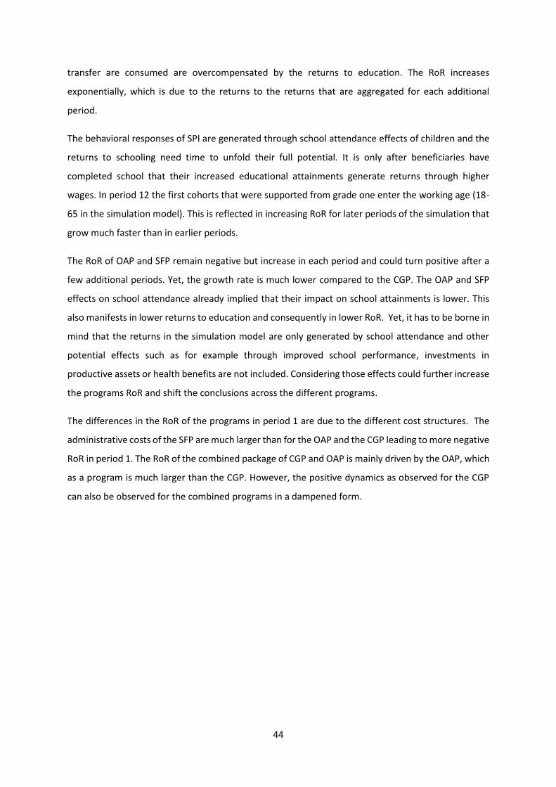
44

transfer are consumed are overcompensated by the returns to education. The RoR increases

exponentially, which is due to the returns to the returns that are aggregated for each additional

period.

The behavioral responses of SPI are generated through school attendance effects of children and the

returns to schooling need time to unfold their full potential. It is only after beneficiaries have

completed school that their increased educational attainments generate returns through higher

wages. In period 12 the first cohorts that were supported from grade one enter the working age (18-

65 in the simulation model). This is reflected in increasing RoR for later periods of the simulation that

grow much faster than in earlier periods.

The RoR of OAP and SFP remain negative but increase in each period and could turn positive after a

few additional periods. Yet, the growth rate is much lower compared to the CGP. The OAP and SFP

effects on school attendance already implied that their impact on school attainments is lower. This

also manifests in lower returns to education and consequently in lower RoR. Yet, it has to be borne in

mind that the returns in the simulation model are only generated by school attendance and other

potential effects such as for example through improved school performance, investments in

productive assets or health benefits are not included. Considering those effects could further increase

the programs RoR and shift the conclusions across the different programs.

The differences in the RoR of the programs in period 1 are due to the different cost structures. The

administrative costs of the SFP are much larger than for the OAP and the CGP leading to more negative

RoR in period 1. The RoR of the combined package of CGP and OAP is mainly driven by the OAP, which

as a program is much larger than the CGP. However, the positive dynamics as observed for the CGP

can also be observed for the combined programs in a dampened form.

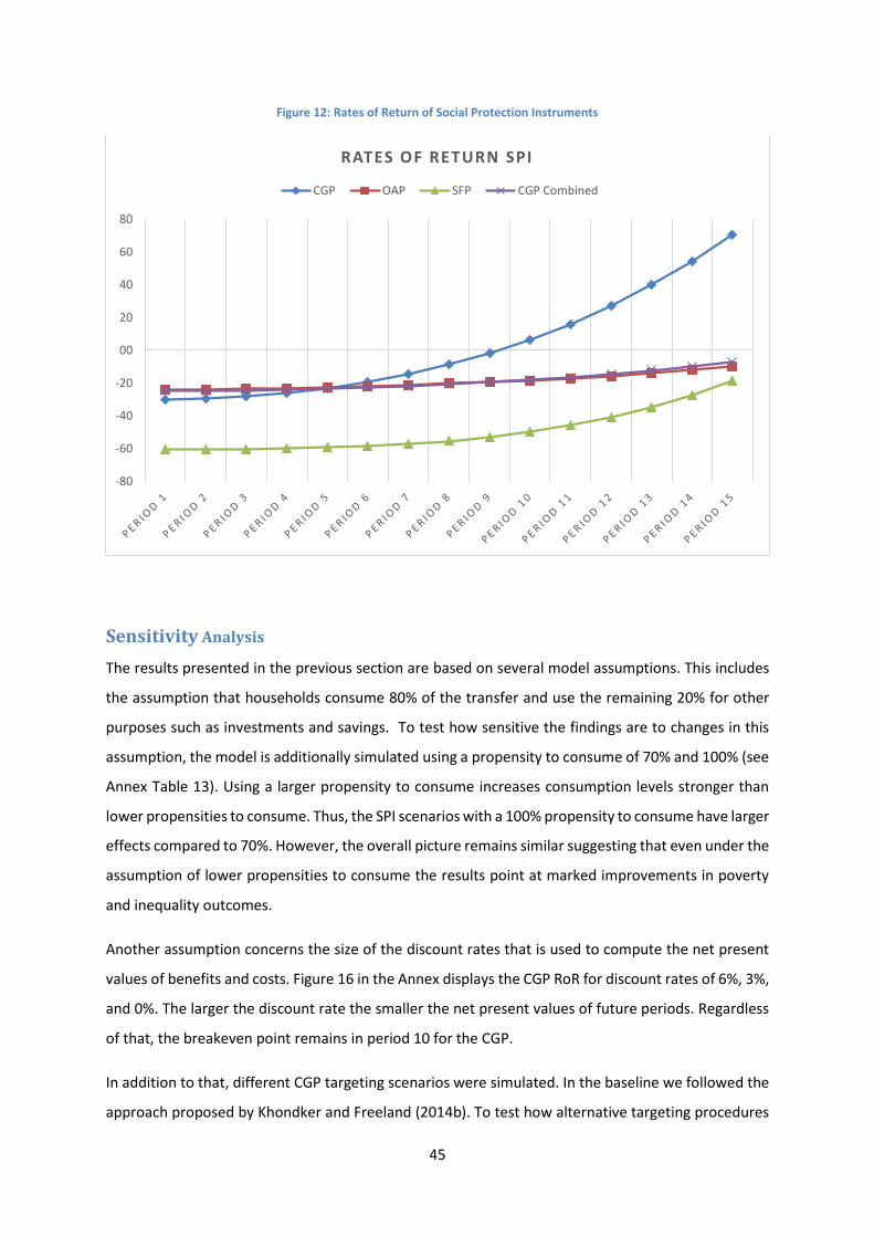
45

Figure 12: Rates of Return of Social Protection Instruments

Sensitivity Analysis

The results presented in the previous section are based on several model assumptions. This includes

the assumption that households consume 80% of the transfer and use the remaining 20% for other

purposes such as investments and savings. To test how sensitive the findings are to changes in this

assumption, the model is additionally simulated using a propensity to consume of 70% and 100% (see

Annex Table 13). Using a larger propensity to consume increases consumption levels stronger than

lower propensities to consume. Thus, the SPI scenarios with a 100% propensity to consume have larger

effects compared to 70%. However, the overall picture remains similar suggesting that even under the

assumption of lower propensities to consume the results point at marked improvements in poverty

and inequality outcomes.

Another assumption concerns the size of the discount rates that is used to compute the net present

values of benefits and costs. Figure 16 in the Annex displays the CGP RoR for discount rates of 6%, 3%,

and 0%. The larger the discount rate the smaller the net present values of future periods. Regardless

of that, the breakeven point remains in period 10 for the CGP.

In addition to that, different CGP targeting scenarios were simulated. In the baseline we followed the

approach proposed by Khondker and Freeland (2014b). To test how alternative targeting procedures

-80

-60

-40

-20

00

20

40

60

80

RATES OF RETURN SPI

CGP OAP SFP CGP Combined

46

could affect outcomes, scenarios for a CGP including also poor households and a universal CGP are

simulated. A summary of outcomes can be found in Annex Table 14. As the effect on school attendance

and thus the returns to education are largest for extremely poor households, the RoR are largest for

the current targeting mechanism. The universal program also generates positive returns at the end of

the simulation period. As a universal program increases the investments markedly, the outcomes also

increase compared to the CGP for extremely poor households. Yet, it has to be noted that we kept the

cost structures identical for all targeting scenarios. Given that a universal targeting would reduce the

(relative) operational costs, the RoR would be larger in each period than presented in Figure 17.

Lastly, the RoR were simulated for a single investment. That means it is tested how an investment in

the first period would affect future consumption levels only through increases in educational

attainments. In this scenario the direct transfer payment of the first period is solely regarded as a cost.

The results show that the educational returns exceed the net present value of transfer payments and

all operational costs after 10 periods. That implies that taking the return to returns into account a one-

time investment in CGP charges off after 10 periods.

7. Conclusion

Lesotho is one of the poorest countries in southern Africa and one of the most unequal economies in

the world (World Bank, 2015a). The depth of poverty makes it difficult for many households to

graduate out of poverty. Besides that, derailing factors such as the HIV/AIDS epidemic are important

sources for persistently high poverty rates and a major source for household’s vulnerability to poverty.

Addressing these challenges, the government of Lesotho expresses the importance of social

protection for achieving these aims by spending about 9% of its GDP on social protection (SP)

programs.

However, despite the large expenditures there is considerable scope for coordination and

harmonization of existing safety net programs. To achieve a more efficient allocation of funds,

evidence is required to guide policymakers in their investment decisions. Using the existing SP funds

more efficiently could benefit the poor and strengthen the efforts to mitigate the consequences of

pervasively high poverty rates in Lesotho.

This simulation study analyzed the short- and mid-term benefits of SPIs in terms of poverty, inequality

and human capital outcomes. In order to contrast the benefits with program costs, the RoR were

computed for a simulated time horizon of 15 years. The simulated benefits include direct transfer

payments and the behavioral responses that are induced by the transfers. This approach allows to

47

examine the direct and indirect returns to SPI and to compare the RoR of different program

interventions.

However, to estimate the RoR several econometric steps are necessary in order to quantify the costs

and benefits. Most essentially the data availability determines the different effect pathways of SPI

that can be considered in the analysis. At the core of the data requirements is a comprehensive

consumption data in order to quantify all benefits and cost. The most current nationally representative

consumption data for Lesotho are from 2002. Moreover, due to data restrictions the indirect benefits

of SPI are limited to returns to education. Other effects, such as for example benefits through

improved health outcomes or agricultural investments cannot be considered in this study.

The analysis of the returns to education suggests that an additional year of schooling increased

consumption levels on average by 9% in 2003. At the same time results of the static simulation model

show that CGP increased the number of years of schooling on average by 2% per year. This highlights

the potential of SPI to generate large returns in future periods. However, the results also showed that

school attainments tend to be low in Lesotho and that the education effects especially on the

extremely poor need more time to unfold their full returns. This results in negative RoR that increased

exponentially and turn positive after 10 periods for the CGP. The simulation results suggest that from

period 10 onwards the CGP generates larger benefits (in net present values) than costs. The RoR of

OAP and SFP remain negative throughout the simulation, but show a positive trend. This finding is

related to the fact that both programs have universal targeting mechanisms and do not particularly

benefit the extremely poor. Secondly, beneficiaries either already attend school (SFP) or left school

age long ago (OAP). Thus, their scope to generate returns through school attendance is much lower

compared to CGP resulting in lower behavioral benefits.

The findings suggest large program effects on poverty and inequality outcomes. Simulating the CGP

on the national level reduced extreme poverty by more than 20% per year and reduced inequality by

up to 7%. This indicates the potential of CGP for poverty reductions in Lesotho. Taking all future

returns into account, the educational benefits exceed all cost including transfers and operational costs

after 10 periods. This underpins the power of SPI for educational but also welfare developments in

Lesotho. On top of that, additional returns through health and agricultural investments and increasing

tax revenues are not considered in this study. Therefore, the results might only reflect a lower bound

estimate of the full potential of social cash transfers.

As a model can never cover the entire set of SPI linkages, it needs to be born in mind that simulation

models are always a simplification of reality. The study has a number of particular limitations that

48

need to be born in mind when interpreting the results. Due to the limitations of the HBS 2002/2003

data, not all potential indirect benefits of social transfers could be incorporated in the model. Effects

through improved health or investments in productive activities are not considered, which may be

particularly important for the OAP. Furthermore, the economic and social situation in Lesotho has

changed considerably since 2002/2003. For example, school attendance and highest education

achievements have increased considerably over the last decade. Nonetheless the models show how

specific aspects of SPI pathways generate monetary returns over the long term.

It is recommend to repeat the present analysis once more comprehensive and more recent household

survey data are available. Particularly the inclusion of other transmission channels next to education

would add value and provide additional insights in the potential benefits and the respective RoR in

the long term. Furthermore, information such as access to services and infrastructure would allow a

more detailed analysis of the returns of SPI which goes beyond the national average and provide

insights into policy areas that need to be strengthened in order to maximize the impact of SPI. The

BOS is keen to improve their data collection and adjust the survey instruments such that they better

serve the overall needs for regular analysis and evaluation of social protection policies.

49

References

Adato, M., and Bassett, L. (2009). ‘Social protection to support vulnerable children and families: the

potential of cash transfers to protect education, health and nutrition’. AIDS Care, 21, 60–75.

Alderman, H. and R. Yemtsov (2012). ‘Productive Role of Safety Nets, Background Paper for the World

Bank 2012–2022 Social Protection and Labor Strategy’, Social Protection & Labor Discussion

Paper, No. 1203, The World Bank, Washington DC.

Arnold et al. (2011). DFID Cash Transfers Evidence Paper. London: Department of International

Development.

Baird, S., Ferreira, F.H.G., Özler, B. and M. Woolcock (2013), ‘Relative Effectiveness of Conditional and

unconditional Cash Transfers for Schooling Outcomes in Developing Countries: A Systematic

Review’. Campbell Systematic Reviews 2013:8 DOI: 10.4073/csr.2013.8

Barber, S. L., & Gertler, P. J. (2008). The impact of Mexico’s conditional cash transfer programme,

Oportunidades, on birthweight. Tropical Medicine & International Health, 13(11), 1405–1414.

Barrientos, A. (2012). ‘Social Transfers and Growth: What Do We Know? What Do We Need to Find

Out?’, World Development, 40(1), pp. 11-20.

Barrientos and Scott (2008); Social Transfers and Growth: A Review. Working Paper, 52, Brooks World

Poverty Institute, University of Manchester.

Bourguignon, Ferreira & Leite (2003). The Poverty-Growth-Inequality Triangle. Policy Research

Working Paper, 28102, The World Bank, Washington DC.

Castells M. and P. Himanen (2002). The Information Society and the Welfare State: The

Finnish Model; Oxford; Oxford University Press

Cherrier, C., Gassmann, F., Mideros Mora, A., and P. Mohnen (2013), ‘Making the investment case for

social protection’, Office of Research Working Paper, WP-2013-06, UNICEF, Florence.

Chirwa, E. et al. (2004). The Evaluation Of The Improving Livelihoods Through Public Works

Programme (ILTPWP). Wadonda Consult/MASAF/CARE Malawi.

Dercon, S. (2011). Social Protection, Efficiency and Growth. Centre for the Study of African Economics,

WPS /2011-17.

50

Devereux, S. and C. Solomon. (2006), Employment Creation Programmes: The International

Experience, Issues in Employment and Poverty, Discussion Paper No. 24, Economic and Labour

Market Analysis Department, International Labour Office (ILO), Geneva.

Gertler, P.J. (2000). The impact of PROGRESA on health. Washington, DC: International Food Policy

Research Institute. Retrieved from

http://ebrary.ifpri.org/cdm/ref/collection/p15738coll2/id/125436

Government of the Kingdom of Lesotho (2015), National Social Protection Strategy.

International Monetary Fund (2015). World Economic Outlook Database October 2015, retrieved from

https://www.imf.org/external/pubs/ft/weo/2015/02/weodata/index.aspx

Khondker, B. and N. Freeland (2014a), Cost estimates of core life‐course schemes proposed under

Lesotho National Social Protection Strategy, mimeo

Khondker and Freeland (2014b). Poverty impacts of core life-course programs proposed under Lesotho

National Social Protection Strategy – A micro simulation exercise, mimeo.

Meng, X., and Ryan, J. (2009). Does a food for education program affect school outcomes? The

Bangladesh case. Journal of Population Economics, 23(2), 415–447.

Mideros, A., Gassmann, F., and P. Mohnen (2012), Estimation of Rates of Return of Social Protection

Investments in Cambodia: A Case for Non-Contributory Social Transfers, UNICEF

Cambodia/Maastricht Graduate School of Governance.

Mideros, A., Gassmann, F., & Mohnen, P. (2015). Estimation of rates of return on social protection: ex

ante microsimulation of social transfers in Cambodia. Journal of Development Effectiveness, 0(0),

1–20.

Miller, C., Tsoka, M., & Reichert, K. (2008). Impact evaluation report: External evaluation of the Mchinji

social cash transfer pilot . Draft. Boston, MA: Center for International Health and Development,

Boston University, and Lilongwe: Center for Social Research, University of Malawi

Mincer, J. A. (1974). Schooling and earnings. In Schooling, experience, and earnings (pp. 41-63). NBER.

51

Ministry of Health (2015), Lesotho Demographic and Health Survey 2014, Maseru: Ministry of Health.

Ministry of Social Development, Lesotho (2014): Policy Brief – Policy Options for the Lesotho Child

Grants Programme, retrieved from http://www.fao.org/3/a-i3848e.pdf

Mwabu, G. and Schultz, T.P. (1996). "Education Returns Across Quantiles of the Wage Function:

Alternative Explanations for Returns to Education by Race in South Africa." American

Economic Review, 86:2, pp. 335-39.

Olivier, M. (2013). Social protection in Lesotho: Innovations and reform challenges. Development

Southern Africa, 30(1), 98–110.

Pellerano et al. (2012). CGP Impact Evaluation –Targeting and baseline evaluation report. Oxford

Policy Management, Oxford, UK

Pellerano et al. (2014). Lesotho Child Grants Programme Impact Evaluation – Follow up report. Oxford

Policy Management, Oxford, UK

Psacharopoulos, G., & Patrinos, H. A. (2004). Returns to investment in education: a further

update. Education economics, 12(2), 111-134.

Samson, M. (2006). Designing and implementing social transfer programmes. EPRI Press.

Samson, M. (2009). Social Cash Transfers and Employment. A note on empirical linkages in developing

countries. In: Promoting pro-poor growth: Employment. OECD Publishing.

Schady, N. (2000). What Education Pays? Non-Linear Returns to Schooling Among Filipino Men. World

Bank.

Schady, N., & Araujo, M. C. (2006). Cash Transfers, Conditions, School Enrollment, And Child Work :

Evidence From A Randomized Experiment In Ecuador. The World Bank.

Schady & Rosero (2008). Are Cash Transfers Made to Women Spent Like Other Sources of Income?

Policy Research Working Paper, 4282, The World Bank, Washington DC.

Stock, J. H., & Yogo, M. (2005). Testing for weak instruments in linear IV regression. Identification and

inference for econometric models: Essays in honor of Thomas Rothenberg.

Tembo, G., Freeland, N., Chimai, B., & Schüring, E. (2014). Social Cash Transfers and Household

Welfare: Evidence from Zambia’s Oldest Scheme. Applied Economics and Finance, 1(1).

52

UNDP (2014). Briefing note for countries on the 2015 Human Development Report: Lesotho.

UNICEF (2012). Lesotho Country Programme Document 2013-2017. Maseru.

World Bank (2010), Lesotho. Sharing Growth by Reducing Inequality and Vulnerability: Choices for

Change. A Poverty, Gender, and Social Assessment, Report #46297-LS, Washington DC: The World

Bank.

World Bank (2013). Lesotho : A Safety Net to End Extreme Poverty. Washington, DC.

World Bank (2015a), Lesotho: Systematic Country Diagnostics, Report #97182, Washington DC: The

World Bank.

World Bank (2015b). Project Appraisal Document on a proposed IDA Credit to the Kingdom of Lesotho

for a Social Assistance Project.

World Bank (2015c). The State of Social Safety Nets 2015. Washington DC: The World Bank.

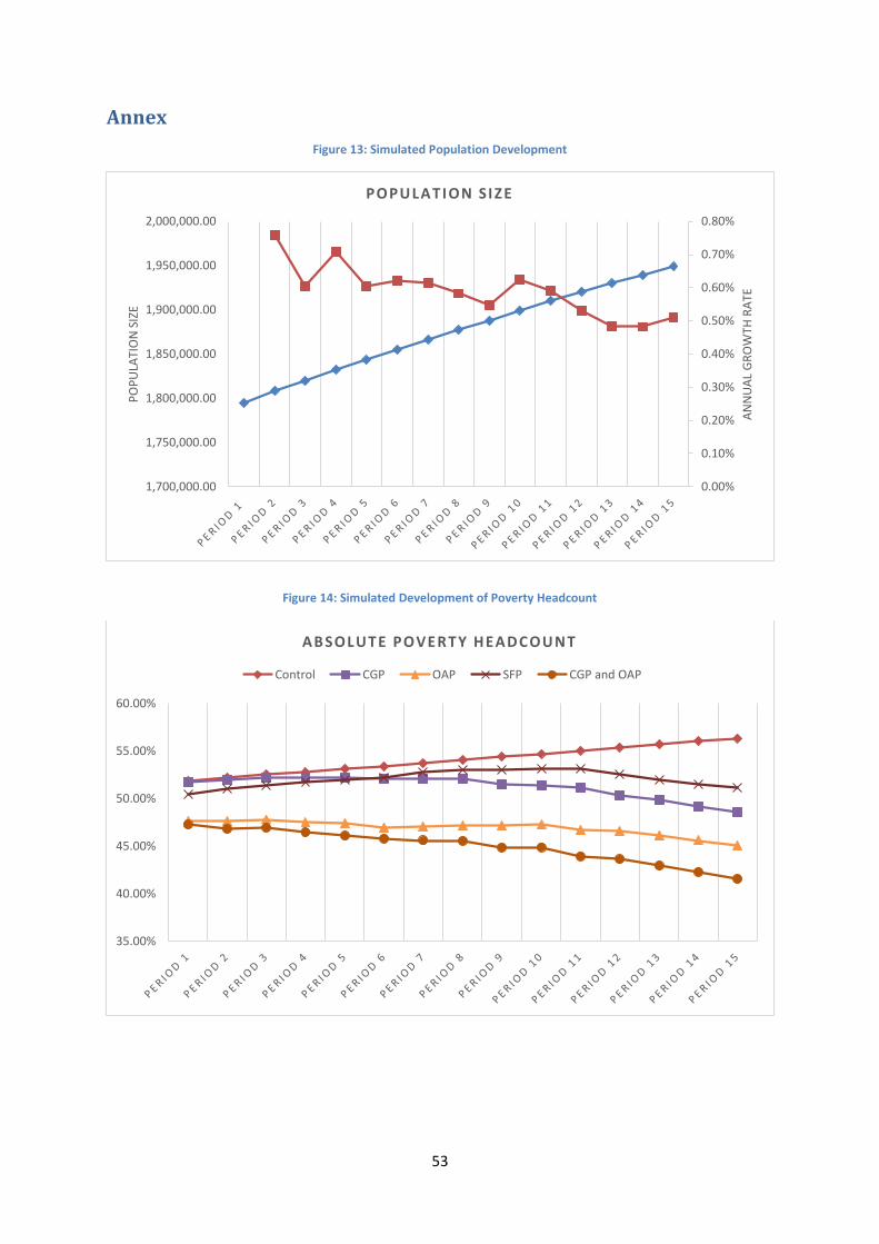
53

Annex

Figure 13: Simulated Population Development

Figure 14: Simulated Development of Poverty Headcount

0.00%

0.10%

0.20%

0.30%

0.40%

0.50%

0.60%

0.70%

0.80%

1,700,000.00

1,750,000.00

1,800,000.00

1,850,000.00

1,900,000.00

1,950,000.00

2,000,000.00

AN

NU

AL

GR

OW

TH R

ATE

PO

PU

LATI

ON

SIZ

E

POPULATION SIZE

35.00%

40.00%

45.00%

50.00%

55.00%

60.00%

ABSOLUTE POVERTY HEADCOUNT

Control CGP OAP SFP CGP and OAP

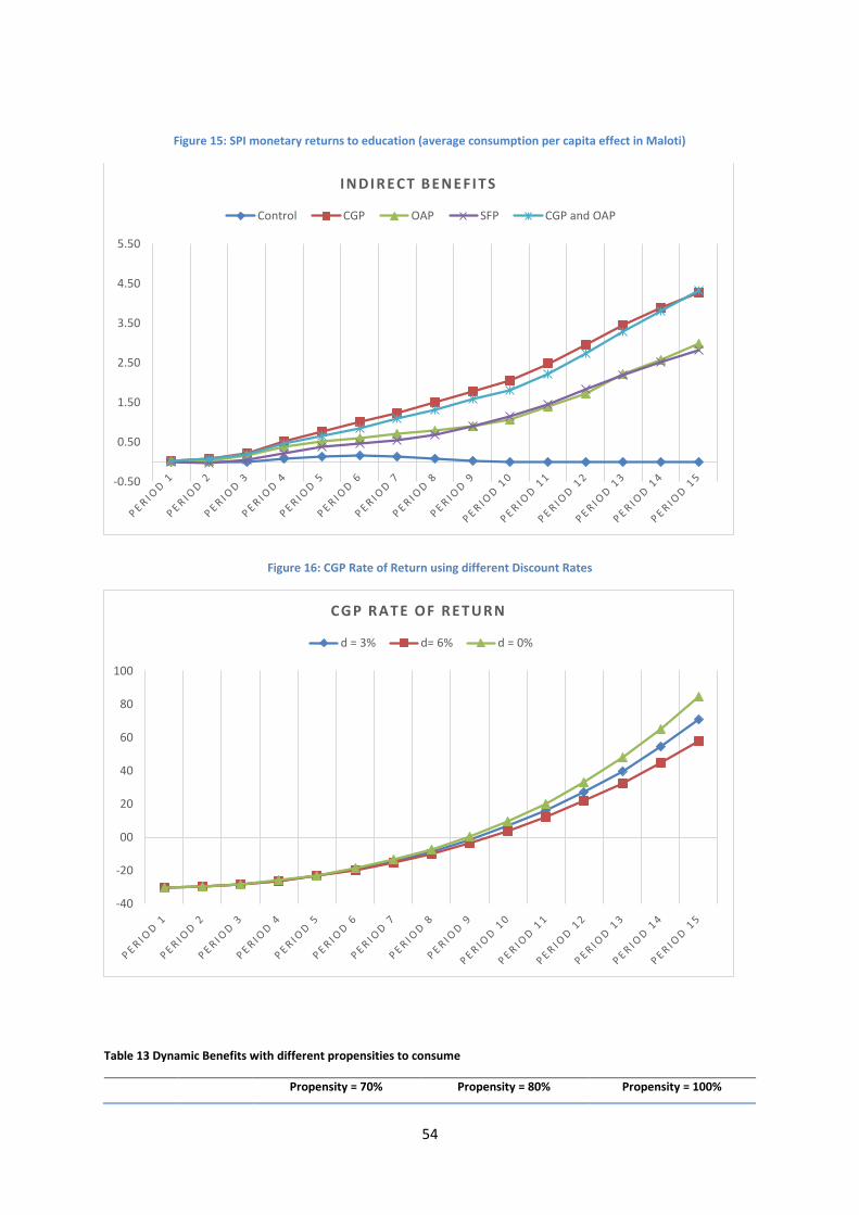
54

Figure 15: SPI monetary returns to education (average consumption per capita effect in Maloti)

Figure 16: CGP Rate of Return using different Discount Rates

Table 13 Dynamic Benefits with different propensities to consume

Propensity = 70% Propensity = 80% Propensity = 100%

-0.50

0.50

1.50

2.50

3.50

4.50

5.50

INDIRECT BENEFITS

Control CGP OAP SFP CGP and OAP

-40

-20

00

20

40

60

80

100

CGP RATE OF RETURN

d = 3% d= 6% d = 0%

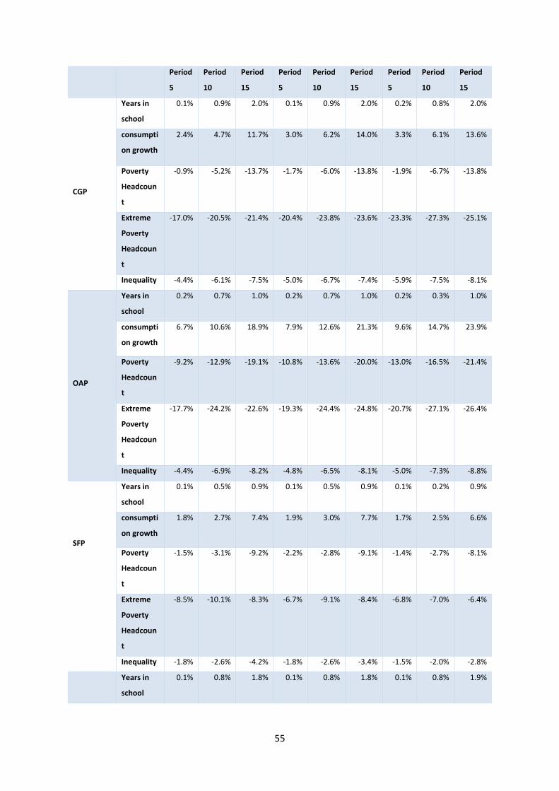
55

Period

5

Period

10

Period

15

Period

5

Period

10

Period

15

Period

5

Period

10

Period

15

CGP

Years in

school

0.1% 0.9% 2.0% 0.1% 0.9% 2.0% 0.2% 0.8% 2.0%

consumpti

on growth

2.4% 4.7% 11.7% 3.0% 6.2% 14.0% 3.3% 6.1% 13.6%

Poverty

Headcoun

t

-0.9% -5.2% -13.7% -1.7% -6.0% -13.8% -1.9% -6.7% -13.8%

Extreme

Poverty

Headcoun

t

-17.0% -20.5% -21.4% -20.4% -23.8% -23.6% -23.3% -27.3% -25.1%

Inequality -4.4% -6.1% -7.5% -5.0% -6.7% -7.4% -5.9% -7.5% -8.1%

OAP

Years in

school

0.2% 0.7% 1.0% 0.2% 0.7% 1.0% 0.2% 0.3% 1.0%

consumpti

on growth

6.7% 10.6% 18.9% 7.9% 12.6% 21.3% 9.6% 14.7% 23.9%

Poverty

Headcoun

t

-9.2% -12.9% -19.1% -10.8% -13.6% -20.0% -13.0% -16.5% -21.4%

Extreme

Poverty

Headcoun

t

-17.7% -24.2% -22.6% -19.3% -24.4% -24.8% -20.7% -27.1% -26.4%

Inequality -4.4% -6.9% -8.2% -4.8% -6.5% -8.1% -5.0% -7.3% -8.8%

SFP

Years in

school

0.1% 0.5% 0.9% 0.1% 0.5% 0.9% 0.1% 0.2% 0.9%

consumpti

on growth

1.8% 2.7% 7.4% 1.9% 3.0% 7.7% 1.7% 2.5% 6.6%

Poverty

Headcoun

t

-1.5% -3.1% -9.2% -2.2% -2.8% -9.1% -1.4% -2.7% -8.1%

Extreme

Poverty

Headcoun

t

-8.5% -10.1% -8.3% -6.7% -9.1% -8.4% -6.8% -7.0% -6.4%

Inequality -1.8% -2.6% -4.2% -1.8% -2.6% -3.4% -1.5% -2.0% -2.8%

Years in

school

0.1% 0.8% 1.8% 0.1% 0.8% 1.8% 0.1% 0.8% 1.9%

56

CGP and

OAP

consumpti

on growth

9.0% 13.9% 23.9% 10.4% 16.3% 27.2% 12.8% 19.7% 32.3%

Poverty

Headcoun

t

-11.5% -16.8% -23.8% -13.2% -17.9% -26.3% -16.1% -22.3% -30.7%

Extreme

Poverty

Headcoun

t

-33.1% -38.4% -37.5% -35.2% -41.5% -40.4% -38.8% -47.3% -46.1%

Inequality -8.3% -10.7% -11.7% -9.0% -11.3% -12.2% -10.1% -12.9% -14.4%

Figure 17: CGP Rate of Return using different Targeting Mechanisms

Table 14 Dynamic Benefits of CGP with different targeting mechanisms

Extreme poor hh with children Poor hh with children All hh with children

Period

5

Period

10

Period

15

Period

5

Period

10

Period

15

Period

5

Period

10

Period

15

Years in

school

0.1% 0.9% 2.0% 0.1% 0.5% 1.4% 0.2% 0.8% 1.8%

consumptio

n growth

per year

3.0% 6.2% 14.0% 3.9% 5.8% 12.4% 6.3% 8.0% 14.7%

Poverty

Headcount

-1.7% -6.0% -13.8% -5.5% -6.2% -13.8% -6.6% -7.9% -15.2%

-40

-20

0

20

40

60

80

CGP RATE OF RETURN: DIFFERENT TARGETING MECHANISMS

Standard Targeting All poor households with children All households with children

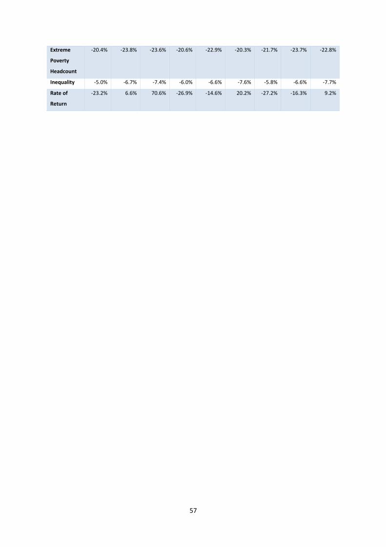
57

Extreme

Poverty

Headcount

-20.4% -23.8% -23.6% -20.6% -22.9% -20.3% -21.7% -23.7% -22.8%

Inequality -5.0% -6.7% -7.4% -6.0% -6.6% -7.6% -5.8% -6.6% -7.7%

Rate of

Return

-23.2% 6.6% 70.6% -26.9% -14.6% 20.2% -27.2% -16.3% 9.2%