ESTIMATION OF (NEAR) LOW-RANK MATRICES WITH NOISE AND …wainwrig/Papers/NegWai11_FullVersion.pdf · estimation of (near) low-rank matrices with noise and high-dimensional scaling

The Annals of Statistics

2011, Vol. 39, No. 2, 1069–1097DOI: 10.1214/10-AOS850© Institute of Mathematical Statistics, 2011

ESTIMATION OF (NEAR) LOW-RANK MATRICES WITH NOISE

AND HIGH-DIMENSIONAL SCALING

BY SAHAND NEGAHBAN AND MARTIN J. WAINWRIGHT1,2

University of California, Berkeley

We study an instance of high-dimensional inference in which the goalis to estimate a matrix �∗ ∈ R

m1×m2 on the basis of N noisy observa-tions. The unknown matrix �∗ is assumed to be either exactly low rank, or“near” low-rank, meaning that it can be well-approximated by a matrix withlow rank. We consider a standard M-estimator based on regularization bythe nuclear or trace norm over matrices, and analyze its performance underhigh-dimensional scaling. We define the notion of restricted strong convexity(RSC) for the loss function, and use it to derive nonasymptotic bounds onthe Frobenius norm error that hold for a general class of noisy observationmodels, and apply to both exactly low-rank and approximately low rank ma-trices. We then illustrate consequences of this general theory for a number ofspecific matrix models, including low-rank multivariate or multi-task regres-sion, system identification in vector autoregressive processes and recovery oflow-rank matrices from random projections. These results involve nonasymp-totic random matrix theory to establish that the RSC condition holds, and todetermine an appropriate choice of regularization parameter. Simulation re-sults show excellent agreement with the high-dimensional scaling of the errorpredicted by our theory.

1. Introduction. High-dimensional inference refers to instances of statisticalestimation in which the ambient dimension of the data is comparable to (or pos-sibly larger than) the sample size. Problems with a high-dimensional characterarise in a variety of applications in science and engineering, including analysis ofgene array data, medical imaging, remote sensing and astronomical data analysis.In settings where the number of parameters may be large relative to the samplesize, the utility of classical (fixed dimension) results is questionable, and accord-ingly, a line of on-going statistical research seeks to obtain results that hold underhigh-dimensional scaling, meaning that both the problem size and sample size (aswell as other problem parameters) may tend to infinity simultaneously. It is usu-ally impossible to obtain consistent procedures in such settings without imposingsome sort of additional constraints. Accordingly, there are now various lines of

Received January 2010; revised August 2010.1Supported in part by a Sloan Foundation Fellowship, Grant AFOSR-09NL184.2Supported by NSF Grants CDI-0941742 and DMS-09-07632.MSC2010 subject classifications. Primary 62F30; secondary 62H12.Key words and phrases. High-dimensional inference, rank constraints, nuclear norm, trace norm,

M-estimators, random matrix theory.

1069

http://www.imstat.org/aos/

http://dx.doi.org/10.1214/10-AOS850

http://www.imstat.org

http://www.ams.org/mathscinet/msc/msc2010.html

1070 S. NEGAHBAN AND M. J. WAINWRIGHT

work on high-dimensional inference based on imposing different types of struc-tural constraints. A substantial body of past work has focused on models withsparsity constraints, including the problem of sparse linear regression [10, 16, 18,36, 50], banded or sparse covariance matrices [7, 8, 19], sparse inverse covariancematrices [24, 44, 48, 55], sparse eigenstructure [2, 30, 42], and sparse regressionmatrices [28, 34, 41, 54]. A theme common to much of this work is the use ofthe ℓ1-penalty as a surrogate function to enforce the sparsity constraint. A parallelline of work has focused on the use of concave penalties to achieve gains in modelselection and sparsity recovery [20, 21].

In this paper, we focus on the problem of high-dimensional inference in the set-ting of matrix estimation. In contrast to past work, our interest in this paper is theproblem of estimating a matrix �∗ ∈ R

m1×m2 that is either exactly low rank, mean-ing that it has at most r ≪ min{m1,m2} nonzero singular values, or more gener-ally is near low-rank, meaning that it can be well-approximated by a matrix of lowrank. As we discuss at more length in the sequel, such exact or approximate low-rank conditions are appropriate for many applications, including multivariate ormulti-task forms of regression, system identification for autoregressive processes,collaborative filtering, and matrix recovery from random projections. Analogousto the use of an ℓ1-regularizer for enforcing sparsity, we consider the use of thenuclear norm (also known as the trace norm) for enforcing a rank constraint in thematrix setting. By definition, the nuclear norm is the sum of the singular values of amatrix, and so encourages sparsity in the vector of singular values, or equivalentlyfor the matrix to be low-rank. The problem of low-rank matrix approximation andthe use of nuclear norm regularization have been studied by various researchers.In her Ph.D. thesis, Fazel [22] discusses the use of nuclear norm as a heuristicfor restricting the rank of a matrix, showing that in practice it is often able toyield low-rank solutions. Other researchers have provided theoretical guaranteeson the performance of nuclear norm and related methods for low-rank matrix ap-proximation. Srebro, Rennie and Jaakkola [49] proposed nuclear norm regulariza-tion for the collaborative filtering problem, and established risk consistency undercertain settings. Recht, Fazel and Parrilo [45] provided sufficient conditions forexact recovery using the nuclear norm heuristic when observing random projec-tions of a low-rank matrix, a set-up analogous to the compressed sensing modelin sparse linear regression [14, 18]. Other researchers have studied a version ofmatrix completion in which a subset of entries are revealed, and the goal is to ob-tain perfect reconstruction either via the nuclear norm heuristic [15] or by otherSVD-based methods [31]. For general observation models, Bach [6] has providedresults on the consistency of nuclear norm minimization in noisy settings, but ap-plicable to the classical “fixed p” setting. In addition, Yuan et al. [53] providenonasymptotic bounds on the operator norm error of the estimate in the multi-tasksetting, provided that the design matrices are orthogonal. Under the assumption ofRIP, Lee and Bresler [32] prove stability properties of least-squares under nuclearnorm constraint when a form of restricted isometry property is imposed on the

NUCLEAR NORM REGULARIZATION 1071

sampling operator. Liu and Vandenberghe [33] develop an efficient interior-pointmethod for solving nuclear-norm constrained problems and illustrate its usefulnessfor problems of system identification, an application also considered in this paper.Finally, in work posted shortly after our own, Rohde and Tsybakov [47] and Can-des and Plan [13] have studied certain aspects of nuclear norm minimization underhigh-dimensional scaling. We discuss connections to this concurrent work at morelength in Section 3.2 following the statement of our main results.

The goal of this paper is to analyze the nuclear norm relaxation for a gen-eral class of noisy observation models and obtain nonasymptotic error bounds onthe Frobenius norm that hold under high-dimensional scaling and are applicableto both exactly and approximately low-rank matrices. We begin by presenting ageneric observation model and illustrating how it can be specialized to the severalcases of interest, including low-rank multivariate regression, estimation of autore-gressive processes and random projection (compressed sensing) observations. Inparticular, this model is specified in terms of an operator X, which may be deter-ministic or random depending on the setting, that maps any matrix �∗ ∈ R

m1×m2

to a vector of N noisy observations. We then present a single main theorem (The-orem 1) followed by two corollaries that cover the cases of exact low-rank con-straints (Corollary 1) and near low-rank constraints (Corollary 2), respectively.These results demonstrate that high-dimensional error rates are controlled by twokey quantities. First, the (random) observation operator X is required to satisfy acondition known as restricted strong convexity (RSC), introduced in a more generalsetting by Negahban et al. [37], which ensures that the loss function has sufficientcurvature to guarantee consistent recovery of the unknown matrix �∗. As we showvia various examples, this RSC condition is weaker than the RIP property, whichrequires that the sampling operator behave very much like an isometry on low-rankmatrices. Second, our theory provides insight into the choice of regularization pa-

rameter that weights the nuclear norm, showing that an appropriate choice is to setit proportionally to the spectral norm of a random matrix defined by the adjoint ofobservation operator X, and the observation noise in the problem.

This initial set of results, though appealing in terms of their simple statementsand generality, are somewhat abstractly formulated. Our next contribution is toshow that by specializing our main result (Theorem 1) to three classes of mod-els, we can obtain some concrete results based on readily interpretable conditions.In particular, Corollary 3 deals with the case of low-rank multivariate regression,relevant for applications in multitask learning. We show that the random opera-tor X satisfies the RSC property for a broad class of observation models, and weuse random matrix theory to provide an appropriate choice of the regularizationparameter. Our next result, Corollary 4, deals with the case of estimating the ma-trix of parameters specifying a vector autoregressive (VAR) process [4, 35]. Theusefulness of the nuclear norm in this context has been demonstrated by Liu andVandenberghe [33]. Here we also establish that a suitable RSC property holdswith high probability for the random operator X, and also specify a suitable choice


of the regularization parameter. We note that the technical details here are con-siderably more subtle than the case of low-rank multivariate regression, due todependencies introduced by the autoregressive sampling scheme. Accordingly, inaddition to terms that involve the size, the matrix dimensions and rank, our boundsalso depend on the mixing rate of the VAR process. Finally, we turn to the com-pressed sensing observation model for low-rank matrix recovery, as introduced byRecht and colleagues [45, 46]. In this setting, we again establish that the RSCproperty holds with high probability, specify a suitable choice of the regulariza-tion parameter and thereby obtain a Frobenius error bound for noisy observations(Corollary 5). A technical result that we prove en route—namely, Proposition 1—is of possible independent interest, since it provides a bound on the constrainednorm of a random Gaussian operator. In particular, this proposition allows us toobtain a sharp result (Corollary 6) for the problem of recovering a low-rank matrixfrom perfectly observed random Gaussian projections with a general dependencystructure.

The remainder of this paper is organized as follows. Section 2 is devoted tobackground material, and the set-up of the problem. We present a generic observa-tion model for low-rank matrices, and then illustrate how it captures various casesof interest. We then define the convex program based on nuclear norm regulariza-tion that we analyze in this paper. In Section 3, we state our main theoretical resultsand discuss their consequences for different model classes. Section 4 is devoted tothe proofs of our results; in each case, we break down the key steps in a seriesof lemmas, with more technical details deferred to the appendices. In Section 5,we present the results of various simulations that illustrate excellent agreementbetween the theoretical bounds and empirical behavior.

NOTATION. For the convenience of the reader, we collect standard piecesof notation here. For a pair of matrices � and Ŵ with commensurate dimen-sions, we let 〈〈�,Ŵ〉〉 = trace(�T Ŵ) denote the trace inner product on matrixspace. For a matrix � ∈ R

m1×m2 , we define m = min{m1,m2}, and denote its(ordered) singular values by σ1(�) ≥ σ2(�) ≥ · · · ≥ σm(�) ≥ 0. We also usethe notation σmax(�) = σ1(�) and σmin(�) = σm(�) to refer to the maximaland minimal singular values, respectively. We use the notation ||| · ||| for varioustypes of matrix norms based on these singular values, including the nuclear norm

|||�|||1 = ∑mj=1 σj (�), the spectral or operator norm |||�|||op = σ1(�), and the

Frobenius norm |||�|||F =√

trace(�T �) =√∑m

j=1 σ 2j (�). We refer the reader to

Horn and Johnson [26, 27] for more background on these matrix norms and theirproperties.

2. Background and problem set-up. We begin with some background onproblems and applications in which rank constraints arise, before describing ageneric observation model. We then introduce the semidefinite program (SDP)based on nuclear norm regularization that we study in this paper.


2.1. Models with rank constraints. Imposing a rank r constraint on a matrix�∗ ∈ R

m1×m2 is equivalent to requiring the rows (or columns) of �∗ lie in somer-dimensional subspace of R

m2 (or Rm1 , resp.). Such types of rank constraints (or

approximate forms thereof) arise in a variety of applications, as we discuss here.In some sense, rank constraints are a generalization of sparsity constraints; ratherthan assuming that the data is sparse in a known basis, a rank constraint implicitlyimposes sparsity but without assuming the basis.

We first consider the problem of multivariate regression, also referred to asmulti-task learning in statistical machine learning. The goal of multivariate regres-

sion is to estimate a prediction function that maps covariates Zj ∈ Rm to multi-

dimensional output vectors Yj ∈ Rm1 . More specifically, let us consider the linear

model, specified by a matrix �∗ ∈ Rm1×m2 , of the form

Ya = �∗Za + Wa for a = 1, . . . , n,(1)

where {Wa}na=1 is an i.i.d. sequence of m1-dimensional zero-mean noise vectors.Given a collection of observations {Za, Ya}na=1 of covariate-output pairs, our goalis to estimate the unknown matrix �∗. This type of model has been used in manyapplications, including analysis of fMRI image data [25], analysis of EEG datadecoding [3], neural response modeling [12] and analysis of financial data. Thismodel and closely related ones also arise in the problem of collaborative filter-ing [49], in which the goal is to predict users’ preferences for items (such as moviesor music) based on their and other users’ ratings of related items. The papers [1, 5]discuss additional instances of low-rank decompositions. In all of these settings,the low-rank condition translates into the existence of a smaller set of “features”that are actually controlling the prediction.

As a second (not unrelated) example, we now consider the problem of systemidentification in vector autoregressive processes (see [35] for detailed background).A vector autoregressive (VAR) process in m-dimensions is a stochastic process{Zt }∞t=1 specified by an initialization Z1 ∈ R

m, followed by the recursion

Zt+1 = �∗Zt + Wt for t = 1,2,3, . . . .(2)

In this recursion, the sequence {Wt }∞t=1 consists of i.i.d. samples of innovationsnoise. We assume that each vector Wt ∈ R

m is zero-mean with covariance matrixC ≻ 0, so that the process {Zt }∞t=1 is zero-mean and has a covariance matrix �

given by the solution of the discrete-time Ricatti equation,

� = �∗�(�∗)T + C.(3)

The goal of system identification in a VAR process is to estimate the unknownmatrix �∗ ∈ R

m×m on the basis of a sequence of samples {Zt }nt=1. In many appli-cation domains, it is natural to expect that the system is controlled primarily by alow-dimensional subset of variables. For instance, models of financial data mighthave an ambient dimension m of thousands (including stocks, bonds, and other fi-nancial instruments), but the behavior of the market might be governed by a much


smaller set of macro-variables (combinations of these financial instruments). Sim-ilar statements apply to other types of time series data, including neural data [12,23], subspace tracking models in signal processing and motion models models incomputer vision. While the form of system identification formulated here assumesdirect observation of the state variables {Zt }nt=1, it is also possible to tackle themore general problem when only noisy versions are observed (e.g., see Liu andVandenberghe [33]). An interesting feature of the system identification problem isthat the matrix �∗, in addition to having low rank, might also be required to satisfysome type of structural constraint (e.g., having a Hankel-type structure), and theestimator that we consider here allows for this possibility.

A third example that we consider in this paper is a compressed sensing observa-tion model, in which one observes random projections of the unknown matrix �∗.This observation model has been studied extensively in the context of estimatingsparse vectors [14, 18], and Recht and colleagues [45, 46] suggested and studied itsextension to low-rank matrices. In their set-up, one observes trace inner products ofthe form 〈〈Xi,�

∗〉〉 = trace(XTi �∗), where Xi ∈ R

m1×m2 is a random matrix [e.g.,filled with standard normal N(0,1) entries], so that 〈〈Xi,�

∗〉〉 is a standard ran-dom projection. In the sequel, we consider this model with a more general familyof random projections involving matrices with dependent entries. Like compressedsensing for sparse vectors, applications of this model include computationally ef-ficient updating in large databases (where the matrix �∗ measures the differencebetween the data base at two different time instants) and matrix denoising.

2.2. A generic observation model. We now introduce a generic observationmodel that will allow us to deal with these different observation models in an uni-fied manner. For pairs of matrices A,B ∈ R

m1×m2 , recall the Frobenius or trace in-ner product 〈〈A,B〉〉 := trace(BAT ). We then consider a linear observation modelof the form

yi = 〈〈Xi,�∗〉〉 + εi for i = 1,2, . . . ,N ,(4)

which is specified by the sequence of observation matrices {Xi}Ni=1 and observa-tion noise {εi}Ni=1. This observation model can be written in a more compact man-ner using operator-theoretic notation. In particular, let us define the observationvector

y = [y1 · · · yN ]T ∈ RN

with a similar definition for ε ∈ RN in terms of {εi}Ni=1. We then use the obser-

vation matrices {Xi}Ni=1 to define an operator X : Rm1×m2 → R

N via [X(�)]i =〈〈Xi,�〉〉. With this notation, the observation model (4) can be re-written as

y = X(�∗) + ε.(5)

Let us illustrate the form of the observation model (5) for some of the applica-tions that we considered earlier.


EXAMPLE 1 (Multivariate regression). Recall the observation model (1) formultivariate regression. In this case, we make n observations of vector pairs(Ya,Za) ∈ R

m1 × Rm2 . Accounting for the m1-dimensional nature of the output,

after the model is scalarized, we receive a total of N = m1n observations. Let usintroduce the quantity b = 1, . . . ,m1 to index the different elements of the output,so that we can write

Yab = 〈〈ebZTa ,�∗〉〉 + Wab for b = 1,2, . . . ,m1.(6)

By re-indexing this collection of N = nm1 observations via the mapping

(a, b) �→ i = (a − 1)m1 + b,

we recognize multivariate regression as an instance of the observation model (4)with observation matrix Xi = ebZ

Ta and scalar observation yi = Yab.

EXAMPLE 2 (Vector autoregressive processes). Recall that a vector autore-gressive (VAR) process is defined by the recursion (2), and suppose that weobserve an n-sequence {Zt }nt=1 produced by this recursion. Since each Zt =[Zt1 · · · Ztm]T is m-variate, the scalarized sample size is N = nm. Lettingb = 1,2, . . . ,m index the dimension, we have

Z(t+1)b = 〈〈ebZTt ,�∗〉〉 + Wtb.(7)

In this case, we re-index the collection of N = nm observations via the mapping

(t, b) �→ i = (t − 1)m + b.

After doing so, we see that the autoregressive problem can be written in the form(4) with yi = Z(t+1)b and observation matrix Xi = ebZ

Tt .

EXAMPLE 3 (Compressed sensing). As mentioned earlier, this is a naturalextension of the compressed sensing observation model for sparse vectors to thecase of low-rank matrices [45, 46]. In a typical form of compressed sensing, theobservation matrix Xi ∈ R

m1×m2 has i.i.d. standard normal N(0,1) entries, so thatone makes observations of the form

yi = 〈〈Xi,�∗〉〉 + εi for i = 1,2, . . . ,N .(8)

By construction, these observations are an instance of the model (4). In the sequel,we study a more general observation model, in which the entries of Xi are allowedto have general Gaussian dependencies. For this problem, the more compact form(5) involves a random Gaussian operator mapping R

m1×m2 to RN , and we study

some of its properties in the sequel.


2.3. Regression with nuclear norm regularization. We now consider an es-timator that is naturally suited to the problems described in the previous sec-tion. Recall that the nuclear or trace norm of a matrix � ∈ R

m1×m2 is given by|||�|||1 = ∑m

j=1 σj (�), corresponding to the sum of its singular values. Given acollection of observations (yi,Xi) ∈ R × R

m1×m2 , for i = 1, . . . ,N from the ob-servation model (4), we consider estimating the unknown �∗ ∈ S by solving thefollowing optimization problem:

� ∈ arg min�∈S

{1

2N‖y − X(�)‖2

2 + λN |||�|||1},(9)

where S is a convex subset of Rm1×m2 , and λN > 0 is a regularization parameter.

When S = Rm1×m2 , the optimization problem (9) can be viewed as the analog of

the Lasso estimator [50], tailored to low-rank matrices as opposed to sparse vec-tors. We include the possibility of a more general convex set S since they arisenaturally in certain applications (e.g., Hankel-type constraints in system identifi-cation [33]). When S is a polytope (with S = R

m1×m2 as a special case), then theoptimization problem (9) can be solved in time polynomial in the sample size N

and the matrix dimensions m1 and m2. Indeed, the optimization problem (9) is aninstance of a semidefinite program [51], a class of convex optimization problemsthat can be solved efficiently by various polynomial-time algorithms [11]. For in-stance, Liu and Vandenberghe [33] develop an efficient interior point method forsolving constrained versions of nuclear norm programs. Moreover, as we discussin Section 5, there are a variety of first-order methods for solving the semidefiniteprogram (SDP) defining our M-estimator [29, 40]. These first-order methods arewell suited to the high-dimensional problems arising in statistical settings, and wemake use of one in performing our simulations.

Like in any typical M-estimator for statistical inference, the regularization pa-rameter λN is specified by the statistician. As part of the theoretical results in thenext section, we provide suitable choices of this parameter so that the estimate �

is close in Frobenius norm to the unknown matrix �∗. The setting of the regular-izer depends on the knowledge of the noise variance. While in general one mightneed to estimate this parameter through cross validation [9, 20], we assume knowl-edge of the noise variance in order to most succinctly demonstrate the empiricalbehavior of our results through the experiments.

3. Main results and some consequences. In this section, we state our mainresults and discuss some of their consequences. Section 3.1 is devoted to resultsthat apply to generic instances of low-rank problems, whereas Section 3.3 is de-voted to the consequences of these results for more specific problem classes,including low-rank multivariate regression, estimation of vector autoregressiveprocesses and recovery of low-rank matrices from random projections.


3.1. Results for general model classes. We begin by introducing the key tech-nical condition that allows us to control the error �−�∗ between an SDP solution� and the unknown matrix �∗. We refer to it as the restricted strong convexity con-dition [37], since it amounts to guaranteeing that the quadratic loss function in theSDP (9) is strictly convex over a restricted set of directions. Letting C ⊆ R

m1×m2

denote the restricted set of directions, we say that the operator X satisfies restrictedstrong convexity (RSC) over the set C if there exists some κ(X) > 0 such that

1

2N‖X()‖2

2 ≥ κ(X)||||||2F for all ∈ C .(10)

We note that analogous conditions have been used to establish error bounds in thecontext of sparse linear regression [10, 17], in which case the set C correspondedto certain subsets of sparse vectors. These types of conditions are weaker thanrestricted isometry properties, since they involve only lower bounds on the opera-tor X, and the constant κ(X) can be arbitrarily small.

Of course, the definition (10) hinges on the choice of the restricted set C . Inorder to specify some appropriate sets for the case of (near) low-rank matrices, werequire some additional notation. Any matrix �∗ ∈ R

m1×m2 has a singular valuedecomposition of the form �∗ = UDV T , where U ∈ R

m1×m1 and V ∈ Rm2×m2

are orthonormal matrices. For each integer r ∈ {1,2, . . . ,m}, we let U r ∈ Rm1×r

and V r ∈ Rm2×r be the sub-matrices of singular vectors associated with the top r

singular values of �∗. We then define the following two subspaces of Rm1×m2 :

A(U r ,V r) := { ∈ Rm1×m2 | row() ⊆ V r and col() ⊆ U r}(11a)

and

B(U r ,V r) := { ∈ Rm1×m2 | row() ⊥ V r and col() ⊥ U r},(11b)

where row() ⊆ Rm2 and col() ⊆ R

m1 denote the row space and column space,respectively, of the matrix . When (U r ,V r) are clear from the context, we adoptthe shorthand notation Ar and Br .

We can now define the subsets of interest. Let �Br denote the projection op-erator onto the subspace Br , and define ′′ = �Br () and ′ = − ′′. For apositive integer r ≤ m = min{m1,m2} and a tolerance parameter δ ≥ 0, considerthe following subset of matrices:

C(r; δ) :={ ∈ R

m1×m2 | ||||||F ≥ δ,

(12)

|||′′|||1 ≤ 3|||′|||1 + 4m∑

j=r+1

σj (�∗)

}.

Note that this set corresponds to matrices for which the quantity |||′′|||1 is rela-tively small compared to − ′′ and the remaining m − r singular values of �∗.


The next ingredient is the choice of the regularization parameter λN used insolving the SDP (9). Our theory specifies a choice for this quantity in terms of theadjoint of the operator X—namely, the operator X

∗ : RN → Rm1×m2 defined by

X∗(ε) :=

N∑

i=1

εiXi .(13)

With this notation, we come to the first result of our paper. It is a deterministicresult, which specifies two conditions—namely, an RSC condition and a choiceof the regularizer—that suffice to guarantee that any solution of the SDP (9) fallswithin a certain radius.

THEOREM 1. Suppose �∗ ∈ S and that the operator X satisfies restricted

strong convexity with parameter κ(X) > 0 over the set C(r; δ), and that the regu-

larization parameter λN is chosen such that λN ≥ 2|||X∗(ε)|||op/N . Then any solu-

tion � to the semidefinite program (9) satisfies

|||� − �∗|||F ≤ max{δ,

32λN

√r

κ(X),

[16λN

∑mj=r+1 σj (�

∗)

κ(X)

]1/2}.(14)

Apart from the tolerance parameter δ, the two main terms in the bound (14)have a natural interpretation. The first term (involving

√r) corresponds to estima-

tion error, capturing the difficulty of estimating a rank r matrix. The second is anapproximation error that describes the gap between the true matrix �∗ and the bestrank r approximation. Understanding the magnitude of the tolerance parameter δ

is a bit more subtle, and it depends on the geometry of the set C(r; δ) and, morespecifically, the inequality

|||′′|||1 ≤ 3|||′|||1 + 4m∑

j=r+1

σj (�∗).(15)

In the simplest case, when �∗ is at most rank r , then we have∑m

j=r+1 σj (�∗) = 0,

so the constraint (15) defines a cone. This cone completely excludes certain direc-tions, and thus it is possible that the operator X, while failing RSC in a globalsense, can satisfy it over the cone. Therefore, there is no need for a nonzero tol-erance parameter δ in the exact low-rank case. In contrast, when �∗ is only ap-proximately low-rank, then the constraint (15) no longer defines a cone; rather, itincludes an open ball around the origin. Thus, if X fails RSC in a global sense, thenit will also fail it under the constraint (15). The purpose of the additional constraint||||||F ≥ δ is to eliminate the open ball centered at the origin, so that it is possiblethat X satisfies RSC over C(r, δ).

Let us now illustrate the consequences of Theorem 1 when the true matrix �∗

has exactly rank r , in which case the approximation error term is zero. For thetechnical reasons mentioned above, it suffices to set δ = 0 in the case of exact rankconstraints, and we thus obtain the following result:


COROLLARY 1 (Exact low-rank recovery). Suppose that �∗ ∈ S has rank r ,and X satisfies RSC with respect to C(r;0). Then as long as λN ≥ 2|||X∗(ε)|||op/N ,any optimal solution � to the SDP (9) satisfies the bound

|||� − �∗|||F ≤ 32√

rλN

κ(X).(16)

Like Theorem 1, Corollary 1 is a deterministic statement on the SDP error.It takes a much simpler form since when �∗ is exactly low rank, then neithertolerance parameter δ nor the approximation term are required.

As a more delicate example, suppose instead that �∗ is nearly low-rank, anassumption that we can formalize by requiring that its singular value sequence{σi(�

∗)}mi=1 decays quickly enough. In particular, for a parameter q ∈ [0,1] and apositive radius Rq , we define the set

Bq(Rq) :={� ∈ R

m1×m2∣∣∣

m∑

i=1

|σi(�)|q ≤ Rq

},(17)

where m = min{m1,m2}. Note that when q = 0, the set B0(R0) corresponds to theset of matrices with rank at most R0.

COROLLARY 2 (Near low-rank recovery). Suppose that �∗ ∈ Bq(Rq) ∩ S ,the regularization parameter is lower bounded as λN ≥ 2|||X∗(ε)|||op/N , and the

operator X satisfies RSC with parameter κ(X) ∈ (0,1] over the set C(Rqλ−qN ; δ).

Then any solution � to the SDP (9) satisfies

|||� − �∗|||F ≤ max{δ,32

√Rq

(λN

κ(X)

)1−q/2}.(18)

Note that the error bound (18) reduces to the exact low rank case (16) whenq = 0 and δ = 0. The quantity λ

−qN Rq acts as the “effective rank” in this setting,

as clarified by our proof in Section 4.2. This particular choice is designed to pro-vide an optimal trade-off between the approximation and estimation error terms inTheorem 1. Since λN is chosen to decay to zero as the sample size N increases,this effective rank will increase, reflecting the fact that as we obtain more samples,we can afford to estimate more of the smaller singular values of the matrix �∗.

3.2. Comparison to related work. Past work by Lee and Bresler [32] providesstability results on minimizing the nuclear norm with a quadratic constraint, orequivalently, performing least-squares with nuclear norm constraints. Their resultsare based on the restricted isometry property (RIP), which is more restrictive thanthan the RSC condition given here; see Examples 4 and 5 for concrete examplesof operators X that satisfy RSC but fail RIP. In our notation, their stability re-sults guarantee that the error |||� − �∗|||F is bounded by a quantity proportional


t := ‖y − X(�∗)‖2/√

N . Given the observation model (5) with a noise vector εin which each entry is i.i.d., zero mean with variance ν2, note that we have t ≈ ν

with high probability. Thus, although such a result guarantees stability, it does notguarantee consistency, since for any fixed noise variance ν2 > 0, the error bounddoes not tend to zero as the sample size N increases. In contrast, our bounds alldepend on the noise and sample size via the regularization parameter, whose opti-mal choice is λ∗

N = 2|||X∗(ε)|||op/N . As will be clarified in Corollaries 3 through 5to follow, for noise ε with variance ν and various choices of X, this regularization

parameter satisfies the scaling λ∗N ≍ ν

√m1+m2

N. Thus, our results guarantee con-

sistency of the estimator, meaning that the error tends to zero as the sample sizeincreases.

As previously noted, some concurrent work [13, 47] has also provided resultson estimation of high-dimensional matrices in the noisy and statistical setting.Rohde and Tsybakov [47] derive results for estimating low-rank matrices basedon a quadratic loss term regularized by the Schatten-q norm for 0 < q ≤ 1. Notethat the nuclear norm (q = 1) is a convex program, whereas the values q ∈ (0,1)

provide analogs on concave regularized least squares [20] in the linear regressionsetting. They provide results on both multivariate regression and matrix comple-tion; most closely related to our work are the results on multivariate regression,which we discuss at more length following Corollary 3 below. On the other hand,Candes and Plan [13] present error rates in the Frobenius norm for estimating ap-proximately low-rank matrices under the compressed sensing model, and we dis-cuss below the connection to our Corollary 5 for this particular observation model.A major difference between our work and this body of work lies in the assumptionsimposed on the observation operator X. All of the papers [13, 32, 47] impose therestricted isometry property (RIP), which requires that all restricted singular val-ues of X very close to 1 (so that it is a near-isometry). In contrast, we require onlythe restricted strong convexity (RSC) condition, which imposes only an arbitrarilysmall but positive lower bound on the operator. It is straightforward to constructoperators X that satisfy RSC while failing RIP, as we discuss in Examples 4 and 5to follow.

3.3. Results for specific model classes. As stated, Corollaries 1 and 2 are fairlyabstract in nature. More importantly, it is not immediately clear how the key under-lying assumption—namely, the RSC condition—can be verified, since it is speci-fied via subspaces that depend on �∗, which is, itself, the unknown quantity thatwe are trying to estimate. Nonetheless, we now show how, when specialized tomore concrete models, these results yield concrete and readily interpretable re-sults. As will be clear in the proofs of these results, each corollary requires over-coming two main technical obstacles: establishing that the appropriate form of theRSC property holds in a uniform sense (so that a priori knowledge of �∗ is notrequired) and specifying an appropriate choice of the regularization parameter λN .


Each of these two steps is nontrivial, requiring some random matrix theory, but theend results are simply stated upper bounds that hold with high probability.

We begin with the case of rank-constrained multivariate regression. As dis-cussed earlier in Example 1, recall that we observe pairs (Yi,Zi) ∈ R

m1 × Rm2

linked by the linear model Yi = �∗Zi + Wi , where Wi ∼ N(0, ν2Im1×m1) is ob-servation noise. Here we treat the case of random design regression, meaning thatthe covariates Zi are modeled as random. In particular, in the following result,we assume that Zi ∼ N(0,�), i.i.d. for some m2-dimensional covariance matrix� ≻ 0. Recalling that σmax(�) and σmin(�) denote the maximum and minimumeigenvalues, respectively, we have the following.

COROLLARY 3 (Low-rank multivariate regression). Consider the random de-

sign multivariate regression model where �∗ ∈ Bq(Rq) ∩ S . There are universal

constants {ci, i = 1,2,3} such that if we solve the SDP (9) with regularization

parameter λN = 10 νm1

√σmax(�)

√(m1+m2)

n, we have

|||� − �∗|||2F ≤ c1

(ν2σmax(�)

σ 2min(�)

)1−q/2

Rq

(m1 + m2

n

)1−q/2

(19)

with probability greater than 1 − c2 exp(−c3(m1 + m2)).

REMARKS. Corollary 3 takes a particularly simple form when � = Im2×m2 :then there exists a constant c′

1 such that |||� − �∗|||2F ≤ c′1ν

2−qRq(m1+m2

n)1−q/2.

When �∗ is exactly low rank—that is, q = 0, and �∗ has rank r = R0—this sim-plifies even further to

|||� − �∗|||2F ≤ c′1ν2r(m1 + m2)

n.

The scaling in this error bound is easily interpretable: naturally, the squarederror is proportional to the noise variance ν2, and the quantity r(m1 + m2) countsthe number of degrees of freedom of a m1 × m2 matrix with rank r . Note that ifwe did not impose any constraints on �∗, then since a m1 × m2 matrix has a totalof m1m2 free parameters, we would expect at best3 to obtain rates of the order

|||� − �∗|||2F = �( ν2m1m2n

). Note that when �∗ is low rank—in particular, whenr ≪ min{m1,m2}—then the nuclear norm estimator achieves substantially fasterrates.4

3To clarify our use of sample size, we can either view the multivariate regression model as con-sisting of n samples with a constant SNR, or as N samples with SNR of order 1/m1. We adopt theformer interpretation here.

4We also note that as stated, the result requires that (m1 + m2) tend to infinity in order for theclaim to hold with high probability. Although such high-dimensional scaling is the primary focus ofthis paper, we note that for application to the classical setting of fixed (m1,m2), the same statement(with different constants) holds with m1 + m2 replaced by logn.


It is worth comparing this corollary to a result on multivariate regression due toRohde and Tsybakov [47]. Their result applies to exactly low-rank matrices (saywith rank r), but provides bounds on general Schatten norms (including the Frobe-nius norm). In this case, it provides a comparable rate when we make the settingq = 0 and R0 = r in the bound (19), namely showing that we require roughlyn ≈ r(m1 + m2) samples, corresponding to the number of degrees of freedom.A significant difference lies in the conditions imposed on the design matrices:whereas their result is derived under RIP conditions on the design matrices, werequire only the milder RSC condition. The following example illustrates the dis-tinction for this model.

EXAMPLE 4 (Failure of RIP for multivariate regression). Under the randomdesign model for multivariate regression, we have

F(�) := E[‖X(�)‖22]

n|||�|||2F=

∑m2j=1 ‖

√��j‖2

2

|||�|||2F,(20)

where �j is the j th row of �. In order for RIP to hold, it is necessary thatquantity F(�) is extremely close to 1—certainly less than two—for all low-rank matrices. We now show that this cannot hold unless � has a small con-dition number. Let v ∈ R

m2 and v′ ∈ Rm2 denote the minimum and maximum

eigenvectors of �. By setting � = e1vT , we obtain a rank one matrix for which

F(�) = σmin(�), and similarly, setting �′ = e1(v′)T yields another rank one ma-

trix for which F(�′) = σmax(�). The preceding discussion applies to the aver-age E[‖X(�)‖2

2]/n, but since the individual matrices matrices Xi are i.i.d. andGaussian, we have

‖X(�)‖22

n= 1

n

n∑

i=1

〈〈Xi,�〉〉2 ≤ 2F(�) = 2σmin(�)

with high probability, using χ2-tail bounds. Similarly, ‖X(�′)‖22/n ≥ (1/2) ×

σmax(�) with high probability. Thus, we have exhibited a pair of rank one ma-trices with |||�|||F = |||�′|||F = 1 for which

‖X(�′)‖22

‖X(�)‖22

≥ 1

4

σmax(�)

σmin(�).

Consequently, unless σmax(�)/σmin(�) ≤ 64, it is not possible for RIP tohold with constant δ ≤ 1/2. In contrast, as our results show, the RSC will holdw.h.p. whenever σmin(�) > 0, and the error is allowed to scale with the ratioσmax(�)/σmin(�).

Next we turn to the case of estimating the system matrix �∗ of an autoregressive(AR) model, as discussed in Example 2.


COROLLARY 4 (Autoregressive models). Suppose that we are given n sam-

ples {Zt }nt=1 from a m-dimensional autoregressive process (2) that is stationary,based on a system matrix that is stable (|||�∗|||op ≤ γ < 1) and approximately low-

rank (�∗ ∈ Bq(Rq) ∩ S ). Then there are universal constants {ci, i = 1,2,3} such

that if we solve the SDP (9) with regularization parameter λN = 2c0|||�|||opm(1−γ )

√mn

, then

any solution � satisfies

|||� − �∗|||2F ≤ c1

[σ 2

max(�)

σ 2min(�)(1 − γ )2

]1−q/2

Rq

(m

n

)1−q/2

(21)

with probability greater than 1 − c2 exp(−c3m).

REMARKS. Like Corollary 3, the result as stated requires that the matrix di-mension m tends to infinity, but the same bounds hold with m replaced by logn,yielding results suitable for classical (fixed dimension) scaling. Second, the factor(m/n)1−q/2, like the analogous term5 in Corollary 3, shows that faster rates areobtained if �∗ can be well approximated by a low rank matrix, namely for choicesof the parameter q ∈ [0,1] that are closer to zero. Indeed, in the limit q = 0, weagain reduce to the case of an exact rank constraint r = R0, and the correspondingsquared error scales as rm/n. In contrast to the case of multivariate regression, theerror bound (21) also depends on the upper bound |||�∗|||op = γ < 1 on the oper-ator norm of the system matrix �∗. Such dependence is to be expected since thequantity γ controls the (in)stability and mixing rate of the autoregressive process.As clarified in the proof, the dependence of the sampling in the AR model alsopresents some technical challenges not present in the setting of multivariate re-gression.

Finally, we turn to the analysis of the compressed sensing model for matrixrecovery, as initially described in Example 3. Although standard compressed sens-ing is based on observation matrices Xi with i.i.d. elements, here we consider amore general model that allows for dependence between the entries of Xi . Firstdefining the quantity M = m1m2, we use vec(Xi) ∈ R

M to denote the vector-ized form of the m1 × m2 matrix Xi . Given a symmetric positive definite ma-trix � ∈ R

M×M , we say that the observation matrix Xi is sampled from the �-ensemble if vec(Xi) ∼ N(0,�). Finally, we define the quantity

ρ2(�) := sup‖u‖2=1,‖v‖2=1

var(uT Xv),(22)

where the random matrix X ∈ Rm1×m2 is sampled from the �-ensemble. In the

special case � = I , corresponding to the usual compressed sensing model, wehave ρ2(I ) = 1.

5The term in Corollary 3 has a factor m1 + m2, since the matrix in that case could be nonsquare ingeneral.


The following result applies to any observation model in which the noise vectorε ∈ R

N satisfies the bound ‖ε‖2 ≤ 2ν√

N for some constant ν. This assumptionthat holds for any bounded noise, and also holds with high probability for anyrandom noise vector with sub-Gaussian entries with parameter ν. [The simplestexample is that of Gaussian noise N(0, ν2).]

COROLLARY 5 (Compressed sensing with dependent sampling). Suppose that

the matrices {Xi}Ni=1 are drawn i.i.d. from the �-Gaussian ensemble, and that the

unknown matrix �∗ ∈ Bq(Rq) ∩ S for some q ∈ (0,1]. Then there are universal

constants ci such that for a sample size N > c1ρ2(�)R

1−q/2q (m1 + m2), any so-

lution � to the SDP (9) with regularization parameter λN = c0ρ(�)ν√

m1+m2N

satisfies the bound

|||� − �∗|||2F ≤ c2Rq

((ν2 ∨ 1)(ρ2(�)/σ 2

min(�))(m1 + m2)

N

)1−q/2

(23)

with probability greater than 1 − c3 exp(−c4(m1 +m2)). In the special case q = 0and �∗ of rank r , we have

|||� − �∗|||2F ≤ c2ρ2(�)ν2

σ 2min(�)

r(m1 + m2)

N.(24)

The central challenge in proving this result is in proving an appropriate formof the RSC property. The following result on the random operator X may be ofindependent interest here:

PROPOSITION 1. Consider the random operator X : Rm1×m2 → RN formed

by sampling from the �-ensemble. Then it satisfies

‖X(�)‖2√N

≥ 1

4

∥∥√� vec(�)∥∥

2 − 12ρ(�)

(√m1

N+

√m2

N

)|||�|||1

(25)for all � ∈ R

m1×m2

with probability at least 1 − 2 exp(−N/32).

The proof of this result, provided in Appendix H, makes use of the Gordon–Slepian inequalities for Gaussian processes, and concentration of measure. As weshow in Section C, it implies the form of the RSC property needed to establishCorollary 5.

In concurrent work, Candes and Plan [13] derived a result similar to Corollary 5for the compressed sensing observation model. Their result applies to matriceswith i.i.d. elements with sub-Gaussian tail behavior. While the analysis given hereis specific to Gaussian random matrices, it allows for general dependence among


the entries. Their result applies only under certain restrictions on the sample sizerelative to matrix dimension and rank, whereas our result holds more generallywithout these extra conditions. Moreover, their proof relies on an application ofRIP, which is in general more restrictive than the RSC condition used in our analy-sis. The following example provides a concrete illustration of a matrix familywhere the restricted isometry constants are unbounded as the rank r grows, butRSC still holds.

EXAMPLE 5 (RSC holds when RIP violated). Here we consider a family ofrandom operators X for which RSC holds with high probability, while RIP fails.Consider generating an i.i.d. collection of design matrices Xi ∈ R

m×m, each of theform

Xi = ziIm×m + Gi for i = 1,2, . . . ,N,(26)

where zi ∼ N(0,1) and Gi ∈ Rm×m is a standard Gaussian random matrix, inde-

pendent of zi . Note that we have vec(Xi) ∼ N(0,�), where the m2 × m2 covari-ance matrix has the form

� = vec(Im×m)vec(Im×m)T + Im2×m2 .(27)

Let us compute the quantity ρ(�) = sup‖u‖2=1,‖v‖2=1 var(uT Xv). By the indepen-dence of z and G in the model (26), we have

ρ(�) ≤ var(z) supu∈Sm1−1,v∈Sm2−1

uT v + supu∈Sm1−1,v∈Sm2−1

var(uT Gv) ≤ 2.

Letting X be the associated random operator, we observe that for any � ∈R

m×m, the independence of zi and Gi implies that

E

[‖X(�)‖22

N

]=

∥∥√� vec(�)∥∥2

2 = trace(�)2 + |||�|||2F ≥ |||�|||2F .

Consequently, Proposition 1 implies that

‖X(�)‖2√N

≥ 1

4|||�|||F − 48

√m

N|||�|||1 for all � ∈ R

m×m(28)

with high probability. As mentioned previously, we show in Section C how thistype of lower bound implies the RSC condition needed for our results.

On the other hand, the random operator can never satisfy RIP (with the rank r

increasing), as the following calculation shows. In this context, RIP requires thatbounds of the form

‖X(�)‖22

N |||�|||2F∈ [1 − δ,1 + δ] for all � with rank at most r ,

where δ ∈ (0,1) is a constant independent of r . Note that the bound (28) impliesthat a lower bound of this form holds as long as N = �(rm). Moreover, this lower


bound cannot be substantially sharpened, since the trace term plays no role formatrices with zero diagonals.

We now show that no such upper bound can ever hold. For a rank 1 ≤ r < m,consider the m × m matrix of the form

Ŵ :=[Ir×r/

√r 0r×(m−r)

0(m−r)×r 0(m−r)×(m−r)

].

By construction, we have |||Ŵ|||F = 1 and trace(Ŵ) = √r . Consequently, we have

E

[‖X(Ŵ)‖22

N

]= trace(Ŵ)2 + |||Ŵ|||2F = r + 1.

The independence of the matrices Xi implies that‖X(Ŵ)‖2

2N

is sharply concentratedaround this expected value, so that we conclude that

‖X(Ŵ)‖22

N |||Ŵ|||2F≥ 1

2[1 + r]

with high probability, showing that RIP cannot hold with upper and lower boundsof the same order.

Finally, we note that Proposition 1 also implies an interesting property of thenull space of the operator X, one which can be used to establish a corollaryabout recovery of low-rank matrices when the observations are noiseless. In par-ticular, suppose that we are given the noiseless observations yi = 〈〈Xi,�

∗〉〉 fori = 1, . . . ,N , and that we try to recover the unknown matrix �∗ by solving theSDP

min�∈R

m1⋉m2|||�|||1 such that 〈〈Xi,�〉〉 = yi for all i = 1, . . . ,N .(29)

This recovery procedure was studied by Recht and colleagues [45, 46] in the spe-cial case that Xi is formed of i.i.d. N(0,1) entries. Proposition 1 allows us to obtaina sharp result on recovery using this method for Gaussian matrices with generaldependencies.

COROLLARY 6 (Exact recovery with dependent sampling). Suppose that the

matrices {Xi}Ni=1 are drawn i.i.d. from the �-Gaussian ensemble, and that �∗ ∈ S

has rank r . Given N > c0ρ2(�)r(m1 + m2) noiseless samples, then with proba-

bility at least 1 − 2 exp(−N/32), the SDP (29) recovers the matrix �∗ exactly.

This result removes some extra logarithmic factors that were included in initialwork [45] and provides the appropriate analog to compressed sensing results forsparse vectors [14, 18]. Note that (like in most of our results) we have made littleeffort to obtain good constants in this result: the important property is that thesample size N scales linearly in both r and m1 +m2. We refer the reader to Recht,Xu and Hassibi [46], who study the standard Gaussian model under the scalingr = �(m) and obtain sharp results on the constants.


4. Proofs. We now turn to the proofs of Theorem 1 and Corollary 1 throughCorollary 4. Owing to space constraints, we leave the proofs of Corollaries 5 and 6to the Appendix. However, we note that these proofs make use of Proposition 1 inorder to establish the respective RSC or restricted null space conditions. In eachcase, we provide the primary steps in the main text, with more technical detailsstated as lemmas and proved in the Appendix.

4.1. Proof of Theorem 1. By the optimality of � and feasibility of �∗ for theSDP (9), we have

1

2N‖y − X(�)‖2

2 + λN |||�|||1 ≤ 1

2N‖y − X(�∗)‖2

2 + λN |||�∗|||1.

Defining the error matrix = �∗ − � and performing some algebra yields theinequality

1

2N‖X()‖2

2 ≤ 1

N〈ε,X()〉 + λN {|||� + |||1 − |||�|||1}.(30)

By definition of the adjoint and Hölder’s inequality, we have

1

N|〈ε,X()〉| = 1

N|〈X∗(ε),〉| ≤ 1

N|||X∗(ε)|||op||||||1.(31)

By the triangle inequality, we have |||� + |||1 − |||�|||1 ≤ ||||||1. Substituting thisinequality and the bound (31) into the inequality (30) yields

1

2N‖X()‖2

2 ≤ 1

N|||X∗(ε)|||op||||||1 + λN ||||||1 ≤ 2λN ||||||1,

where the second inequality makes use of our choice λN ≥ 2N

|||X∗(ε)|||op.It remains to lower bound the term on the left-hand side, while upper bounding

the quantity ||||||1 on the right-hand side. The following technical result allows usto do so. Recall our earlier definition (11) of the sets A and B associated with agiven subspace pair.

LEMMA 1. Let U r ∈ Rm1×r and V r ∈ R

m2×r be matrices consisting of the

top r left and right (respectively) singular vectors of �∗. Then there exists a matrix

decomposition = ′ + ′′ of the error such that:

(a) the matrix ′ satisfies the constraint rank(′) ≤ 2r ;(b) if λN ≥ 2|||X∗(ε)|||op/N , then the nuclear norm of ′′ is bounded as

|||′′|||1 ≤ 3|||′|||1 + 4m∑

j=r+1

σj (�∗).(32)


See Appendix B for the proof of this claim. Using Lemma 1, we can completethe proof of the theorem. In particular, from the bound (32) and the RSC assump-tion, we find that for ||||||F ≥ δ, we have

1

2N‖X()‖2

2 ≥ κ(X)||||||2F .

Using the triangle inequality together with inequality (32), we obtain

||||||1 ≤ |||′|||1 + |||′′|||1 ≤ 4|||′|||1 + 4m∑

j=r+1

σj (�∗).

From the rank constraint in Lemma 1(a), we have |||′|||1 ≤√

2r|||′|||F . Puttingtogether the pieces, we find that either ||||||F ≤ δ or

κ(X)||||||2F ≤ max

{32λN

√r||||||F ,16λN

m∑

j=r+1

σj (�∗)

},

which implies that

||||||F ≤ max{δ,

32λN

√r

κ(X),

(16λN

∑mj=r+1 σj (�

∗)

κ(X)

)1/2}

as claimed.

4.2. Proof of Corollary 2. Let m = min{m1,m2}. In this case, we consider thesingular value decomposition �∗ = UDV T , where U ∈ R

m1×m and V ∈ Rm2×m

are orthogonal, and we assume that D is diagonal with the singular values in non-increasing order σ1(�

∗) ≥ σ2(�∗) ≥ · · ·σm(�∗) ≥ 0. For a parameter τ > 0 to be

chosen, we define

K := {i ∈ {1,2, . . . ,m} | σi(�

∗) > τ},

and we let UK (resp., V K ) denote the m1 × |K| (resp., the m2 × |K|) orthogo-nal matrix consisting of the first |K| columns of U (resp., V ). With this choice,the matrix �∗

Kc := �B|K|(�∗) has rank at most m − |K|, with singular values{σi(�

∗), i ∈ Kc}. Moreover, since σi(�∗) ≤ τ for all i ∈ Kc, we have

|||�∗Kc |||1 = τ

m∑

i=|K|+1

σi(�∗)

τ≤ τ

m∑

i=|K|+1

(σi(�

∗)τ

)q

≤ τ 1−qRq .

On the other hand, we also have Rq ≥ ∑mi=1 |σi(�

∗)|q ≥ |K|τ q , which impliesthat |K| ≤ τ−qRq . From the general error bound with r = |K|, we obtain

|||� − �∗|||F ≤ max{δ,

32λN

√Rqτ−q/2

κ(X),

[16λNτ 1−qRq

κ(X)

]1/2}.


Setting τ = λN/κ(X) yields that

|||� − �∗|||F ≤ max{δ,

32λ1−q/2N

√Rq

κ1−q/2,

[16λ

2−qN Rq

κ2−q

]1/2}

= max{δ,32

√Rq

(λN

κ(X)

)1−q/2}

as claimed.

4.3. Proof of Corollary 3. For the proof of this corollary, we adopt the follow-ing notation. We first define the three matrices

X =

⎡⎢⎢⎣

ZT1

ZT2

· · ·ZT

n

⎤⎥⎥⎦ ∈ R

n×m2, Y =

⎡⎢⎢⎣

Y T1

Y T2

· · ·Y T

n

⎤⎥⎥⎦ ∈ R

n×m1 and

(33)

W =

⎡⎢⎢⎣

W T1

W T2

· · ·W T

n

⎤⎥⎥⎦ ∈ R

n×m1 .

With this notation and using the relation N = nm1, the SDP objective function(9) can be written as 1

m1{ 1

2n|||Y − X�T |||2F + λn|||�|||1}, where we have defined

λn = λNm1.In order to establish the RSC property for this model, some algebra shows that

we need to establish a lower bound on the quantity

1

2n|||X|||2F = 1

2n

m∑

j=1

‖(X)j‖22 ≥ σmin(X

T X)

2n||||||2F ,

where σmin denotes the minimum eigenvalue. The following lemma follows byadapting known concentration results for random matrices (see [52] for details):

LEMMA 2. Let X ∈ Rn×m be a random matrix with i.i.d. rows sampled from

a m-variate N(0,�) distribution. Then for n ≥ 2m, we have

P

[σmin

(1

nXT X

)≥ σmin(�)

9, σmax

(1

nXT X

)≤ 9σmax(�)

]≥ 1 − 4 exp(−n/2).

As a consequence, we have σmin(XT X)

2n≥ σmin(�)

18 with probability at least 1 −4 exp(−n) for all n ≥ 2m, which establishes that the RSC property holds withκ(X) = 1

20m1σmin(�).


Next we need to upper bound the quantity |||X∗(ε)|||op for this model, so as toverify that the stated choice for λN is valid. Following some algebra, we find that

1

n|||X∗(ε)|||op = 1

n|||XT W |||op.

The following lemma is proved in Appendix F:

LEMMA 3. There are constants ci > 0 such that

P

[∣∣∣∣1

n|||XT W |||op

∣∣∣∣ ≥ 5ν√

σmax(�)

√m1 + m2

n

]≤ c1 exp

(−c2(m1 + m2)).(34)

Using these two lemmas, we can complete the proof of Corollary 3. First, re-calling the scaling N = m1n, we see that Lemma 3 implies that the choice λn =10ν

√σmax(�)

√m1+m2

nsatisfies the conditions of Corollary 2 with high probabil-

ity. Lemma 2 shows that the RSC property holds with κ(X) = σmin(�)/(20m1),again with high probability. Consequently, Corollary 2 implies that

|||� − �∗|||2F ≤ 322Rq

(10ν

√σmax(�)

√m1 + m2

n

20

σmin(�)

)2−q

= c1

(ν2σmax(�)

σ 2min(�)

)1−q/2

Rq

(m1 + m2

n

)1−q/2

with probability greater than 1 − c2 exp(−c3(m1 + m2)), as claimed.

4.4. Proof of Corollary 4. For the proof of this corollary, we adopt the notation

X =

⎡⎢⎢⎣

ZT1

ZT2

· · ·ZT

n

⎤⎥⎥⎦ ∈ R

n×m and Y =

⎡⎢⎢⎣

ZT2

ZT2

· · ·ZT

n+1

⎤⎥⎥⎦ ∈ R

n×m.

Finally, we let W ∈ Rn×m be a matrix where each row is sampled i.i.d. from

the N(0,C) distribution corresponding to the innovations noise driving the VARprocess. With this notation, and using the relation N = nm, the SDP objectivefunction (9) can be written as 1

m{ 1

2n|||Y − X�T |||2F +λn|||�|||1}, where we have de-

fined λn = λNm. At a high level, the proof of this corollary is similar to that ofCorollary 3, in that we use random matrix theory to establish the required RSCproperty and to justify the choice of λn, or equivalently λN . However, it is con-siderably more challenging, due to the dependence in the rows of the random ma-trices, and the cross-dependence between the two matrices X and W (which wereindependent in the setting of multivariate regression).

The following lemma provides the lower bound needed to establish RSC for theautoregressive model:


LEMMA 4. The eigenspectrum of the matrix XT X/n is well controlled in

terms of the stationary covariance matrix: in particular, as long as n > c3m, we

have

σmax

((1

nXT X

))(a)≤ 24σmax(�)

1 − γand σmin

((1

nXT X

))(b)≥ σmin(�)

4,(35)

both with probability greater than 1 − 2c1 exp(−c2m).

Thus, from the bound (35)(b), we see with the high probability, the RSC prop-erty holds with κ(X) = σmin(�)/(4m2) as long as n > c3m.

As before, in order to verify the choice of λn, we need to control the quantity1n|||XT W |||op. The following inequality, proved in Appendix G.2, yields a suitable

upper bound:

LEMMA 5. There exist constants ci > 0, independent of n,m,� etc. such that

P

[1

n|||XT W |||op ≥ c0|||�|||op

1 − γ

√m

n

]≤ c2 exp(−c3m).(36)

From Lemma 5, we see that it suffices to choose λn = 2c0|||�|||op1−γ

√mn

. With thischoice, Corollary 2 of Theorem 1 yields that

|||� − �∗|||2F ≤ c1Rq

[σmax(�)

σmin(�)(1 − γ )

]2−q(m

n

)1−q/2

with probability greater than 1 − c2 exp(−c3m), as claimed.

5. Experimental results. In this section, we report the results of various sim-ulations that demonstrate the close agreement between the scaling predicted byour theory, and the actual behavior of the SDP-based M-estimator (9) in practice.In all cases, we solved the convex program (9) by using our own implementa-tion in MATLAB of an accelerated gradient descent method which adapts a non-smooth convex optimization procedure [40] to the nuclear-norm [29]. We chosethe regularization parameter λN in the manner suggested by our theoretical re-sults; in doing so, we assumed knowledge of the noise variance ν2. In practice,one would have to estimate such quantities from the data using methods such ascross-validation, as has been studied in the context of the Lasso, and we leave thisas an interesting direction for future research.

We report simulation results for three of the running examples discussed inthis paper: low-rank multivariate regression, estimation in vector autoregressiveprocesses and matrix recovery from random projections (compressed sensing). Ineach case, we solved instances of the SDP for a square matrix �∗ ∈ R

m×m, wherem ∈ {40,80,160} for the first two examples, and m ∈ {20,40,80} for the com-pressed sensing example. In all cases, we considered the case of exact low rank


FIG. 1. Results of applying the SDP (9) with nuclear norm regularization to the problem of

low-rank multivariate regression. (a) Plots of the Frobenius error |||� − �∗|||F on a logarithmic

scale versus the sample size N for three different matrix sizes m2 ∈ {1600,6400,25600}, all with

rank r = 10. (b) Plots of the same Frobenius error versus the rescaled sample size N/(rm). Consis-

tent with theory, all three plots are now extremely well aligned.

constraints, with rank(�∗) = r = 10, and we generated �∗ by choosing the sub-spaces of its left and right singular vectors uniformly at random from the Grassmanmanifold.6 The observation noise had variance ν2 = 1, and we chose C = ν2I forthe VAR process. The VAR process was generated by first solving for the covari-ance matrix � using the MATLAB function dylap and then generating a samplepath. For each setting of (r,m), we solved the SDP for a range of sample sizes N .

Figure 1 shows results for a multivariate regression model with the covariateschosen randomly from a N(0, I ) distribution. Panel (a) plots the Frobenius error|||� − �∗|||F on a logarithmic scale versus the sample size N for three differentmatrix sizes, m ∈ {40,80,160}. Naturally, in each case, the error decays to zeroas N increases, but larger matrices require larger sample sizes, as reflected by therightward shift of the curves as m is increased. Panel (b) of Figure 1 shows theexact same set of simulation results, but now with the Frobenius error plotted ver-sus the rescaled sample size N := N/(rm). As predicted by Corollary 3, the errorplots now are all aligned with one another; the degree of alignment in this particu-lar case is so close that the three plots are now indistinguishable. (The blue curveis the only one visible since it was plotted last by our routine.) Consequently, Fig-ure 1 shows that N/(rm) acts as the effective sample size in this high-dimensionalsetting.

Figure 2 shows similar results for the autoregressive model discussed in Ex-ample 2. As shown in panel (a), the Frobenius error again decays as the sample

6More specifically, we let �∗ = XY T , where X,Y ∈ Rm×r have i.i.d. N(0,1) elements.


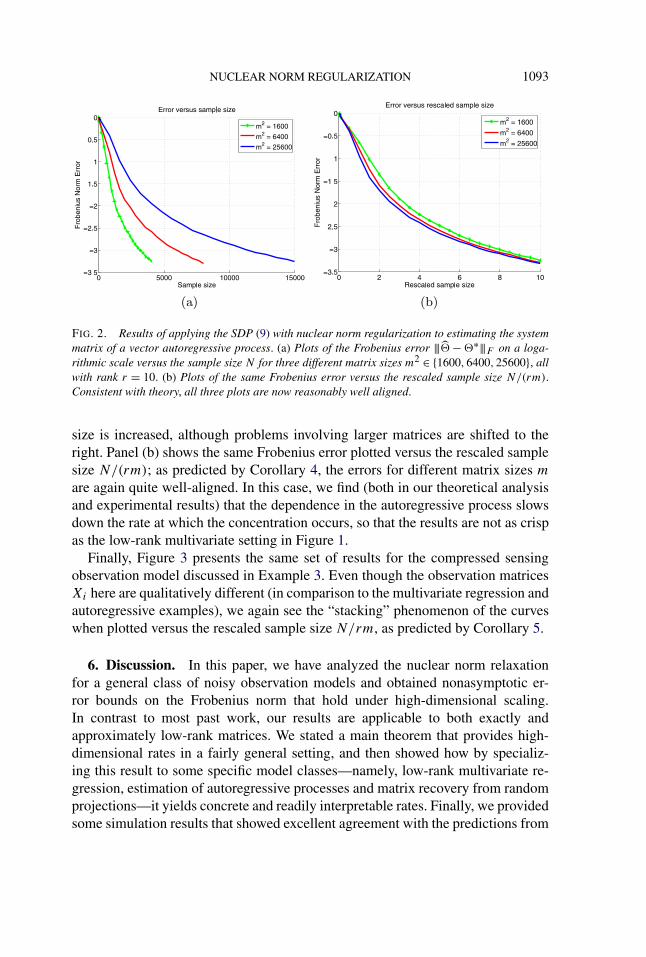
FIG. 2. Results of applying the SDP (9) with nuclear norm regularization to estimating the system

matrix of a vector autoregressive process. (a) Plots of the Frobenius error |||� − �∗|||F on a loga-

rithmic scale versus the sample size N for three different matrix sizes m2 ∈ {1600,6400,25600}, all

with rank r = 10. (b) Plots of the same Frobenius error versus the rescaled sample size N/(rm).Consistent with theory, all three plots are now reasonably well aligned.

size is increased, although problems involving larger matrices are shifted to theright. Panel (b) shows the same Frobenius error plotted versus the rescaled samplesize N/(rm); as predicted by Corollary 4, the errors for different matrix sizes m

are again quite well-aligned. In this case, we find (both in our theoretical analysisand experimental results) that the dependence in the autoregressive process slowsdown the rate at which the concentration occurs, so that the results are not as crispas the low-rank multivariate setting in Figure 1.

Finally, Figure 3 presents the same set of results for the compressed sensingobservation model discussed in Example 3. Even though the observation matricesXi here are qualitatively different (in comparison to the multivariate regression andautoregressive examples), we again see the “stacking” phenomenon of the curveswhen plotted versus the rescaled sample size N/rm, as predicted by Corollary 5.

6. Discussion. In this paper, we have analyzed the nuclear norm relaxationfor a general class of noisy observation models and obtained nonasymptotic er-ror bounds on the Frobenius norm that hold under high-dimensional scaling.In contrast to most past work, our results are applicable to both exactly andapproximately low-rank matrices. We stated a main theorem that provides high-dimensional rates in a fairly general setting, and then showed how by specializ-ing this result to some specific model classes—namely, low-rank multivariate re-gression, estimation of autoregressive processes and matrix recovery from randomprojections—it yields concrete and readily interpretable rates. Finally, we providedsome simulation results that showed excellent agreement with the predictions from


FIG. 3. Results of applying the SDP (9) with nuclear norm regularization to recovering a low-rank

matrix on the basis of random projections (compressed sensing model). (a) Plots of the Frobenius er-

ror |||� − �∗|||F on a logarithmic scale versus the sample size N for three different matrix sizes

m2 ∈ {400,1600,6400}, all with rank r = 10. (b) Plots of the same Frobenius error versus the

rescaled sample size N/(rm). Consistent with theory, all three plots are now reasonably well aligned.

our theory. Our more recent work has also shown that this same framework can beused to obtain near-optimal bounds for the matrix completion problem [38].

This paper has focused on achievable results for low-rank matrix estimationusing a particular polynomial-time method. It would be interesting to establishmatching lower bounds, showing that the rates obtained by this estimator areminimax-optimal. We suspect that this should be possible, for instance, by usingthe techniques exploited in Raskutti, Wainwright and Yu [43] in analyzing mini-max rates for regression over ℓq -balls.

Acknowledgments. We thank the editors and anonymous reviewers for theirconstructive comments.

SUPPLEMENTARY MATERIAL

Supplement to “Estimation of (Near) Low-Rank Matrices with Noise and

High-Dimensional Scaling” (DOI: 10.1214/10-AOS850SUPP; .pdf). Owing tospace constraints, we have moved many of the technical proofs and details to theAppendix, which is contained in the supplementary document [39].

REFERENCES

[1] ABERNETHY, J., BACH, F., EVGENIOU, T. and STEIN, J. (2006). Low-rank matrix factorizationwith attributes. Technical Report N-24/06/MM, Ecole des mines de Paris, France.

[2] AMINI, A. A. and WAINWRIGHT, M. J. (2009). High-dimensional analysis of semidefiniterelaxations for sparse principal components. Ann. Statist. 37 2877–2921. MR2541450

http://dx.doi.org/10.1214/10-AOS850SUPP

http://www.ams.org/mathscinet-getitem?mr=2541450


[3] ANDERSON, C. W., STOLZ, E. A. and SHAMSUNDER, S. (1998). Multivariate autoregressivemodels for classification of spontaneous electroencephalogram during mental tasks. IEEE

Trans. Bio-Med. Eng. 45 277.[4] ANDERSON, T. W. (1971). The Statistical Analysis of Time Series. Wiley, New York.

MR0283939[5] ARGYRIOU, A., EVGENIOU, T. and PONTIL, M. (2006). Multi-task feature learning. In Neural

Information Processing Systems (NIPS) 41–48. Vancouver, Canada.[6] BACH, F. (2008). Consistency of trace norm minimization. J. Mach. Learn. Res. 9 1019–1048.

MR2417263[7] BICKEL, P. and LEVINA, E. (2008). Covariance estimation by thresholding. Ann. Statist. 36

2577–2604. MR2485008[8] BICKEL, P. and LEVINA, E. (2008). Regularized estimation of large covariance matrices. Ann.

Statist. 36 199–227. MR2387969[9] BICKEL, P. and LI, B. (2006). Regularization in statistics. TEST 15 271–344. MR2273731

[10] BICKEL, P., RITOV, Y. and TSYBAKOV, A. (2009). Simultaneous analysis of Lasso and Dantzigselector. Ann. Statist. 37 1705–1732. MR2533469

[11] BOYD, S. and VANDENBERGHE, L. (2004). Convex Optimization. Cambridge Univ. Press,Cambridge. MR2061575

[12] BROWN, E. N., KASS, R. E. and MITRA, P. P. (2004). Multiple neural spike train data analysis:State-of-the-art and future challenges. Nature Neuroscience 7 456–466.

[13] CANDÈS, E. and PLAN, Y. (2010). Tight oracle bounds for low-rank matrix recovery from aminimal number of random measurements. Technical report, Stanford Univ. Available atarXiv:1001.0339v1.

[14] CANDES, E. and TAO, T. (2005). Decoding by linear programming. IEEE Trans. Inform. Theory

51 4203–4215. MR2243152[15] CANDÈS, E. J. and RECHT, B. (2009). Exact matrix completion via convex optimization.

Found. Comput. Math. 9 717–772. MR2565240[16] CHEN, S., DONOHO, D. L. and SAUNDERS, M. A. (1998). Atomic decomposition by basis

pursuit. SIAM J. Sci. Comput. 20 33–61. MR1639094[17] COHEN, A., DAHMEN, W. and DEVORE, R. (2009). Compressed sensing and best k-term ap-

proximation. J. Amer. Math. Soc. 22 211–231. MR2449058[18] DONOHO, D. (2006). Compressed sensing. IEEE Trans. Inform. Theory 52 1289–1306.

MR2241189[19] EL-KAROUI, N. (2008). Operator norm consistent estimation of large dimensional sparse co-

variance matrices. Ann. Statist. 36 2717–2756. MR2485011[20] FAN, J. and LI, R. (2001). Variable selection via non-concave penalized likelihood and its oracle

properties. J. Amer. Statist. Assoc. 96 1348–1360. MR1946581[21] FAN, J. and LV, J. (2010). A selective overview of variable selection in high dimensional feature

space. Statist. Sinica 20 101–148. MR2640659[22] FAZEL, M. (2002). Matrix Rank Minimization with Applications. Ph.D. thesis, Stanford Univ.

Available at http://faculty.washington.edu/mfazel/thesis-final.pdf.[23] FISHER, J. and BLACK, M. J. (2005). Motor cortical decoding using an autoregressive moving

average model. 27th Annual International Conference of the Engineering in Medicine and

Biology Society, 2005. IEEE-EMBS 2005 2130–2133.[24] FRIEDMAN, J., HASTIE, T. and TIBSHIRANI, R. (2007). Sparse inverse covariance estimation

with the graphical Lasso. Biostatistics 9 432–441.[25] HARRISON, L., PENNY, W. D. and FRISTON, K. (2003). Multivariate autoregressive modeling

of fmri time series. NeuroImage 19 1477–1491.[26] HORN, R. A. and JOHNSON, C. R. (1985). Matrix Analysis. Cambridge Univ. Press, Cambridge.

MR0832183








http://arxiv.org/abs/arXiv:1001.0339v1









http://faculty.washington.edu/mfazel/thesis-final.pdf



[27] HORN, R. A. and JOHNSON, C. R. (1991). Topics in Matrix Analysis. Cambridge Univ. Press,Cambridge. MR1091716

[28] HUANG, J. and ZHANG, T. (2009). The benefit of group sparsity. Technical report, RutgersUniv. Available at arXiv:0901.2962.

[29] JI, S. and YE, J. (2009). An accelerated gradient method for trace norm minimization. In Inter-

national Conference on Machine Learning (ICML) 457–464. ACM, New York.[30] JOHNSTONE, I. M. (2001). On the distribution of the largest eigenvalue in principal components

analysis. Ann. Statist. 29 295–327. MR1863961[31] KESHAVAN, R. H., MONTANARI, A. and OH, S. (2009). Matrix completion from noisy entries.

Technical report, Stanford Univ. Available at http://arxiv.org/abs/0906.2027v1.[32] LEE, K. and BRESLER, Y. (2009). Guaranteed minimum rank approximation from linear ob-

servations by nuclear norm minimization with an ellipsoidal constraint. Technical report.UIUC. Available at arXiv:0903.4742.

[33] LIU, Z. and VANDENBERGHE, L. (2009). Interior-point method for nuclear norm optimiza-tion with application to system identification. SIAM J. Matrix Anal. Appl. 31 1235–1256.MR2558821

[34] LOUNICI, K., PONTIL, M., TSYBAKOV, A. B. and VAN DE GEER, S. (2009). Taking ad-vantage of sparsity in multi-task learning. Technical report, ETH Zurich. Available atarXiv:0903.1468.

[35] LÜTKEPOLHL, H. (2006). New Introduction to Multiple Time Series Analysis. Springer, NewYork.

[36] MEINSHAUSEN, N. and BÜHLMANN, P. (2006). High-dimensional graphs and variable selec-tion with the Lasso. Ann. Statist. 34 1436–1462. MR2278363

[37] NEGAHBAN, S., RAVIKUMAR, P., WAINWRIGHT, M. J. and YU, B. (2009). A unified frame-work for high-dimensional analysis of M-estimators with decomposable regularizers. InProceedings of the NIPS Conference 1348–1356. Vancouver, Canada.

[38] NEGAHBAN, S. and WAINWRIGHT, M. J. (2010). Restricted strong convexity and (weighted)matrix completion: Near-optimal bounds with noise. Technical report, Univ. California,Berkeley.

[39] NEGAHBAN, S. and WAINWRIGHT, M. J. (2010). Supplement to “Estimation of (near) low-rank matrices with noise and high-dimensional scaling.” DOI:10.1214/10-AOS850SUPP.

[40] NESTEROV, Y. (2007). Gradient methods for minimizing composite objective function. Tech-nical Report 2007/76, CORE, Univ. Catholique de Louvain.

[41] OBOZINSKI, G., WAINWRIGHT, M. J. and JORDAN, M. I. (2011). Union support recovery inhigh-dimensional multivariate regression. Ann. Statist. 39 1–47.

[42] PAUL, D. and JOHNSTONE, I. (2008). Augmented sparse principal component analysis for high-dimensional data. Technical report, Univ. California, Davis.

[43] RASKUTTI, G., WAINWRIGHT, M. J. and YU, B. (2009). Minimax rates of estimation forhigh-dimensional linear regression over ℓq -balls. Technical report, Dept. Statistics, Univ.California, Berkeley. Available at arXiv:0910.2042.

[44] RAVIKUMAR, P., WAINWRIGHT, M. J., RASKUTTI, G. and YU, B. (2008). High-dimensionalcovariance estimation: Convergence rates of ℓ1-regularized log-determinant divergence.Technical report, Dept. Statistics, Univ. California, Berkeley.

[45] RECHT, B., FAZEL, M. and PARRILO, P. A. (2010). Guaranteed minimum-rank solutions oflinear matrix equations via nuclear norm minimization. SIAM Rev. 52 471–501.

[46] RECHT, B., XU, W. and HASSIBI, B. (2009). Null space conditions and thresholds for rankminimization. Technical report, Univ. Wisconsin–Madison. Available at http://pages.cs.wisc.edu/~brecht/papers/10.RecXuHas.Thresholds.pdf.

[47] ROHDE, A. and TSYBAKOV, A. (2011). Estimation of high-dimensional low-rank matrices.Ann. Statist. 39 887–930.


http://arxiv.org/abs/arXiv:0901.2962


http://arxiv.org/abs/0906.2027v1





http://dx.doi.org/10.1214/10-AOS850SUPP


http://pages.cs.wisc.edu/~brecht/papers/10.RecXuHas.Thresholds.pdf

http://pages.cs.wisc.edu/~brecht/papers/10.RecXuHas.Thresholds.pdf


[48] ROTHMAN, A. J., BICKEL, P. J., LEVINA, E. and ZHU, J. (2008). Sparse permutation invariantcovariance estimation. Electronic J. Statist. 2 494–515. MR2417391

[49] SREBRO, N., RENNIE, J. and JAAKKOLA, T. (2005). Maximum-margin matrix factorization. InProceedings of the NIPS Conference 1329–1336. Vancouver, Canada.

[50] TIBSHIRANI, R. (1996). Regression shrinkage and selection via the Lasso. J. Roy. Statist. Soc.

Ser. B 58 267–288. MR1379242[51] VANDENBERGHE, L. and BOYD, S. (1996). Semidefinite programming. SIAM Rev. 38 49–95.

MR1379041[52] WAINWRIGHT, M. J. (2009). Sharp thresholds for high-dimensional and noisy sparsity recov-

ery using ℓ1-constrained quadratic programming (Lasso). IEEE Trans. Inform. Theory 55

2183–2202.[53] YUAN, M., EKICI, A., LU, Z. and MONTEIRO, R. (2007). Dimension reduction and coefficient

estimation in multivariate linear regression. J. R. Stat. Soc. Ser. B Stat. Methodol. 69 329–346. MR2323756

[54] YUAN, M. and LIN, Y. (2006). Model selection and estimation in regression with groupedvariables. J. R. Stat. Soc. Ser. B Stat. Methodol. 68 49–67. MR2212574

[55] YUAN, M. and LIN, Y. (2007). Model selection and estimation in the Gaussian graphical model.Biometrika 94 19–35. MR2367824

DEPARTMENT OF ELECTRICAL ENGINEERING

UNIVERSITY OF CALIFORNIA, BERKELEY

BERKELEY, CALIFORNIA 94720USAE-MAIL: [email protected]

DEPARTMENT OF STATISTICS

UNIVERSITY OF CALIFORNIA, BERKELEY

BERKELEY, CALIFORNIA 94720USAE-MAIL: [email protected]







mailto:[email protected]

mailto:[email protected]

Submitted to the Annals of Statistics

SUPPLEMENTARY MATERIAL FOR: ESTIMATION OF(NEAR) LOW-RANK MATRICES WITH NOISE AND

HIGH-DIMENSIONAL SCALING

By Sahand Negahban and Martin J. Wainwright


APPENDIX A: INTRODUCTION

In this supplement we present many of the technical details from themain work [1]. Equation or theorem references made to the main documentare relative to the numbering scheme of the document and will not containletters.

APPENDIX B: PROOF OF LEMMA 1

Part (a) of the claim was proved in Recht et al. [2]; we simply providea proof here for completeness. We write the SVD as Θ∗ = UDV T , whereU ∈ R

m1×m1 and V ∈ Rm2×m2 are orthogonal matrices, and D is the matrix

formed by the singular values of Θ∗. Note that the matrices U r and V r aregiven by the first r columns of U and V respectively. We then define thematrix Γ = UT ΔV ∈ R

m1×m2 , and write it in block form as

Γ =

[Γ11 Γ12

Γ21 Γ22

], where Γ11 ∈ R

r×r, and Γ22 ∈ R(m1−r)×(m2−r).

We now define the matrices

Δ′′ = U

[0 00 Γ22

]V T , and Δ′ = Δ − Δ′′.

Note that we have

rank(Δ′) = rank

[Γ11 Γ12

Γ21 0

]≤ rank

[Γ11 Γ12

0 0

]+ rank

[Γ11 0Γ21 0

]≤ 2r,

which establishes Lemma 1(a). Moreover, we note for future reference thatby construction of Δ′′, the nuclear norm satisfies the decomposition

|||ΠAr (Θ∗) + Δ′′|||1 = |||ΠAr(Θ∗)|||1 + |||Δ′′|||1.(B.1)

1imsart-aos ver. 2010/08/03 file: RR_AOS_Sahand_trim.tex date: November 16, 2010


We now turn to the proof of Lemma 1(b). Recall that the error Δ = Θ−Θ∗

associated with any optimal solution must satisfy the inequality (30), whichimplies that

0 ≤ 1

N〈�ε, X(Δ)〉 + λN

{|||Θ∗|||1 − |||Θ|||1

}≤ ||| 1

NX∗(�ε)|||op |||Δ|||1 + λN

{|||Θ∗|||1 − |||Θ|||1

},

(B.2)

where we have used the bound (31).Note that we have the decomposition Θ∗ = ΠAr (Θ∗) + ΠBr(Θ∗). Using

this decomposition, the triangle inequality and the relation (B.1), we have

|||Θ|||1 = |||(ΠAr (Θ∗) + Δ′′) + (ΠBr(Θ∗) + Δ′)|||1≥ |||(ΠAr (Θ∗) + Δ′′)|||1 − |||(ΠBr (Θ∗) + Δ′)|||1≥ |||ΠAr (Θ∗)|||1 + |||Δ′′|||1 −

{|||(ΠBr (Θ∗)|||1 + |||Δ′|||1

}.

Consequently, we have

|||Θ∗|||1 − |||Θ|||1 ≤ |||Θ∗|||1 −{|||ΠAr (Θ∗)|||1 + |||Δ′′|||1

}+{|||(ΠBr (Θ∗)|||1 + |||Δ′|||1

}

= 2|||ΠBr (Θ∗)|||1 + |||Δ′|||1 − |||Δ′′|||1.Substituting this inequality into the bound (B.2), we obtain

0 ≤ ||| 1

NX∗(�ε)|||op |||Δ|||1 + λN

{2|||ΠBr (Θ∗)|||1 + |||Δ′|||1 − |||Δ′′|||1

}.

Finally, since ||| 1N X

∗(�ε)|||op ≤ λN/2 by assumption, we conclude that

0 ≤ λN{2|||ΠBr (Θ∗)|||1 +

3

2|||Δ′|||1 −

1

2|||Δ′′|||1

}.

Since |||ΠBr(Θ∗)|||1 =∑m

j=r+1 σj(Θ∗), the bound (32) follows.

APPENDIX C: PROOF OF COROLLARY 5

Recall that for this model, the observations are of the form yi = 〈〈Xi, Θ∗〉〉+εi, where Θ∗ ∈ R

m1×m2 is the unknown matrix, and {εi}Ni=1 is an associated

noise sequence.We now show how Proposition 1 implies the RSC property with an appro-

priate tolerance parameter δ > 0 to be defined. Observe that the bound (25)implies that for any Δ ∈ C, we have

‖X(Δ)‖2√N

≥√

σmin(Σ)

4|||Δ|||F − 12ρ(Σ)

(√m1

N+

√m2

N

)|||Δ|||1

=

√σmin(Σ)

4

{|||Δ|||F − 48ρ(Σ)√

σmin(Σ)

(√m1

N+

√m2

N

)

︸︷︷︸τ

|||Δ|||1}

,(C.1)

imsart-aos ver. 2010/08/03 file: RR_AOS_Sahand_trim.tex date: November 16, 2010

NUCLEAR NORM MINIMIZATION SUPPLEMENTARY MATERIAL 3

where we have defined the quantity τ > 0. Following the arguments used inthe proofs of Theorem 1 and Corollary 2, we find that

|||Δ|||1 ≤ 4|||Δ′|||1 + 4m∑

j=r+1

σj(Θ∗) ≤ 4

√2Rqτ−q |||Δ′|||F + 4Rqτ

1−q.

(C.2)

Note that this corresponds to truncating the matrices at effective rank r =2Rqτ

−q. Combining this bound with the definition of τ , we obtain

τ |||Δ|||1 ≤ 4√

2Rqτ1−q/2 |||Δ′|||F + 4Rqτ

2−q ≤ 4√

2Rqτ1−q/2 |||Δ|||F + 4Rqτ

2−q.

Substituting this bound into equation (C.1) yields

‖X(Δ)‖2√N

≥√

σmin(Σ)

4

{|||Δ|||F − 4

√2Rqτ

1−q/2 |||Δ′|||F − 4Rqτ2−q}

.

As long N > c0R2/(2−q)q

ρ2(Σ)σmin(Σ) (m1 +m2) for a sufficiently large constant c0,

we can ensure that 4√

2Rqτ1−q/2 < 1/2, and hence that

‖X(Δ)‖2√N

≥√

σmin(Σ)

4

{1

2|||Δ|||F − 4Rqτ

2−q}

.

Consequently, if we define δ := 16Rqτ2−q, then we are guaranteed that for

all |||Δ|||F ≥ δ, we have 4Rqτ2−q ≤ |||Δ|||F /4, and hence

‖X(Δ)‖2√N

≥√

σmin(Σ)

16|||Δ|||F

for all |||Δ|||F ≥ δ. We have thus shown that C(2Rqτ−q; δ) with parameter

κ(X) = σmin(Σ)256 .

The next step is to control the quantity |||X∗(�ε)|||op/N , required for speci-fying a suitable choice of λN .

Lemma C.1. If ‖�ε‖2 ≤ 2ν√

N , then there are universal constants ci suchthat

P

[ |||X∗(�ε)|||opN

≥ c0ρ(Σ)ν

(√m1

N+

√m2

N

)]≤ c1 exp(−c2(m1 + m2)).(C.3)



Proof. By the definition of the adjoint operator, we have Z = 1N X

∗(�ε) =1N

∑Ni=1 εiXi. Since the observation matrices {Xi}N

i=1 are i.i.d. Gaussian, ifthe sequence {εi}N

i=1 is viewed as fixed (by conditioning as needed), then therandom matrix Z is a sample from the Γ-ensemble with covariance matrix

Γ = ‖�ε‖2

N2 Σ 2ν2

N Σ. Therefore, letting Z ∈ Rm1×m2 be a random matrix

drawn from the 2ν2Σ/N -ensemble, we have

P[|||Z|||op ≥ t

]≤ P

[|||Z|||op ≥ t].

Using Lemma H.1 from Appendix H, we have

E[|||Z|||op] ≤ 12√

2νρ(Σ)√N

(√m1 +

√m2)

and

P[|||Z|||op ≥ E[|||Z|||op] + t

]≤ exp

(− c1

Nt2

ν2ρ2(Σ)

)

for a universal constant c1. Setting t2 = Ω(ν2ρ2(Σ)(

√m1+

√m2)2

N yields theclaim.

APPENDIX D: PROOF OF COROLLARY 6

This corollary follows from a combination of Proposition 1 and Lemma 1.Let Θ be an optimal solution to the SDP (29), and let Δ = Θ − Θ∗ be theerror. Since Θ is optimal and Θ∗ is feasible for the SDP, we have |||Θ|||1 =|||Θ∗ + Δ|||1 ≤ |||Θ∗|||1. Using the decomposition Δ = Δ′ + Δ′′ from Lemma 1and applying triangle inequality, we have

|||Θ∗ + Δ′ + Δ′′|||1 ≥ |||Θ∗ + Δ′′|||1 − |||Δ′|||1.

From the properties of the decomposition in Lemma 1 (see Appendix B),we find that

|||Θ|||1 = |||Θ∗ + Δ′ + Δ′′|||1 ≥ |||Θ∗|||1 + |||Δ′′|||1 − |||Δ′|||1.

Combining the pieces yields that |||Δ′′|||1 ≤ |||Δ′|||1, and hence |||Δ|||1 ≤ 2|||Δ′|||1.By Lemma 1(a), the rank of Δ′ is at most 2r, so that we obtain |||Δ|||1 ≤2√

2r|||Δ|||F ≤ 4√

r|||Δ|||F .



Note that X(Δ) = 0, since both Θ and Θ∗ agree with the observations.Consequently, from Proposition 1, we have that

0 =‖X(Δ)‖2√

N≥ 1

4|||Δ|||F − 12ρ(Σ)

(√m1

N+

√m2

N

)|||Δ|||1

≥ |||Δ|||F(

1

4− 12ρ(Σ)

√rm1

N+ 12ρ(Σ)

√rm2

N

)

≥ 1

20|||Δ|||F

where the final inequality as long as N > c0ρ2(Σ)r(m1+m2) for a sufficiently

large constant c0. We have thus shown that Δ = 0, which implies thatΘ = Θ∗ as claimed.

APPENDIX E: CONSISTENCY IN OPERATOR NORM

In this appendix, we derive a bound on the operator norm error for boththe low-rank multivariate regression and auto-regressive model estimationproblems. In this statement, it is convenient to specify these models in theform Y = XΘ∗ + W , where Y ∈ R

n×m2 is a matrix of observations.

Proposition E.1 (Operator norm consistency). Consider the multi-variate regression problem and the SDP under the conditions of Corollary 3.Then any solution Θ to the SDP satisfies the bound

|||Θ − Θ∗|||op ≤ c′ν√

σmax(Σ)

σmin(Σ)

√m1 + m2

n.(E.1)

We note that a similar bound applies to the auto-regressive model treatedin Corollary 4.

Proof. For any subgradient matrix Z ∈ ∂|||Θ|||1, we are guaranteed|||Z|||op ≤ 1. Furthermore, by the KKT conditions [3] for the nuclear normSDP, any solution Θ must satisfy the condition

1

nXT XΘ − XT Y

n+ λnZ = 0.

Hence, simple algebra and the triangle inequality yield that

|||Θ|||op ≤ |||( 1n

XT X)−1|||op

[|||XT W/n|||op + λn

].



Lemma 2 yields that |||(

1nXT X

)−1|||op ≤ 9σmin(Σ) with high probability. Com-

bining these inequalities yields

|||Θ|||op ≤ c1λn

σmin(Σ).

We require that λn ≥ 2|||XT W |||op/n. From Lemma 3, it suffices to set λn ≥c0

√σmax(Σ)ν

√m1+m2

n . Combining the pieces yields the claim.

APPENDIX F: PROOF OF LEMMA 3

Let Sm−1 = {u ∈ Rm | ‖u‖2 = 1} denote the Euclidean sphere in m-

dimensions. The operator norm of interest has the variational representation

1

n|||XT W |||op =

1

nsup

u∈Sm1−1

supv∈Sm2−1

vT XT Wu

For positive scalars a and b, define the (random) quantity

Ψ(a, b) := supu∈a Sm1−1

supv∈b Sm2−1

〈Xv, Wu〉.

and note that our goal is to upper bound Ψ(1, 1). Note moreover thatΨ(a, b) = a bΨ(1, 1), a relation which will be useful in the analysis.

Let A = {u1, . . . , uA} and B = {v1, . . . , vB} denote 1/4 coverings of Sm1−1

and Sm2−1, respectively. We now claim that we have the upper bound

(F.1) Ψ(1, 1) ≤ 4 maxua∈A,vb∈B

〈Xvb, Wua〉

To establish this claim, we note that since the sets A and B are 1/4-covers,for any pair (u, v) ∈ Sm−1 × Sm−1, there exists a pair (ua, vb) ∈ A × Bsuch that u = ua + Δu and v = vb + Δv, with max{‖Δu‖2, ‖Δv‖2} ≤ 1/4.Consequently, we can write

〈Xv, Wu〉 = 〈Xvb, Wua〉 + 〈Xvb, WΔu〉 + 〈XΔv, Wua〉 + 〈XΔv, WΔu〉.(F.2)

By construction, we have the bound |〈Xvb, WΔu〉| ≤ Ψ(1, 1/4) = 14Ψ(1, 1),

and similarly |〈XΔv, Wua〉| ≤ 14Ψ(1, 1) as well as |〈XΔv, WΔu〉| ≤ 1

16Ψ(1, 1).Substituting these bounds into the decomposition (F.2) and taking supremaover the left and right-hand sides, we conclude that

Ψ(1, 1) ≤ maxua∈A,vb∈B

〈Xvb, Wua〉 +9

16Ψ(1, 1),



from which the bound (F.1) follows.We now apply the union bound to control the discrete maximum. It is

known (e.g., [4, 5]) that there exists a 1/4 covering of Sm1−1 and Sm2−1

with at most A ≤ 8m1 and B ≤ 8m2 elements respectively. Consequently, wehave

P[|Ψ(1, 1)| ≥ 4δ n

]≤ 8m1+m2 max

ua,vbP

[|〈Xvb, Wua〉|

n≥ δ

].(F.3)

It remains to obtain a good bound on the quantity 1n〈Xv, Wu〉 = 1

n

∑ni=1〈v, Xi〉〈u, Wi〉,

where (u, v) ∈ Sm1−1 × Sm2−1 are arbitrary but fixed. Since Wi ∈ Rm1 has

i.i.d. N(0, ν2) elements and u is fixed, we have Zi : = 〈u, Wi〉 ∼ N(0, ν2)for each i = 1, . . . , n. These variables are independent of one another, andof the random matrix X. Therefore, conditioned on X, the sum Z : =1n

∑ni=1〈v, Xi〉〈u, Wi〉 is zero-mean Gaussian with variance

α2 : =ν2

n

(1

n‖Xv‖2

2

)≤ ν2

n|||XT X/n|||op.

Define the event T = {α2 ≤ 9ν2|||Σ|||opn }. Using Lemma 2, we have |||XT X/n|||op ≤

9σmax(Σ) with probability at least 1 − 2 exp(−n/2), which implies thatP[T c] ≤ 2 exp(−n/2). Therefore, conditioning on the event T and its com-plement T c, we obtain

P[|Z| ≥ t] ≤ P[|Z| ≥ t | T

]+ P[T c]

≤ exp

(−n

t2

2ν2 (4 + |||Σ|||op)

)+ 2exp(−n/2).

Combining this tail bound with the upper bound (F.3), we have

P[|ψ(1, 1)| ≥ 4δ n

]≤ 8m1+m2

{exp

(−n

t2

18ν2|||Σ|||op

)+ 2exp(−n/2)

}.

Setting t2 = 20ν2|||Σ|||op m1+m2

n , this probability vanishes as long as n >16(m1 + m2).

APPENDIX G: TECHNICAL DETAILS FOR COROLLARY 4

In this appendix, we collect the proofs of Lemmas 4 and 5.



G.1. Proof of Lemma 4. Recalling that Sm−1 denotes the unit-normEuclidean sphere in m-dimensions, we first observe that |||X|||op = supu∈Sm−1 ‖Xu‖2.Our next step is to reduce the supremum to a maximization over a finiteset, using a standard covering argument. Let A = {u1, . . . , uA} denote a 1/2-cover of it. By definition, for any u ∈ Sm−1, there is some ua ∈ A such thatu = ua + Δu, where ‖Δu‖2 ≤ 1/2. Consequently, for any u ∈ Sm−1, thetriangle inequality implies that

‖Xu‖2 ≤ ‖Xua‖2 + ‖XΔu‖2,

and hence that |||X|||op ≤ maxua∈A ‖Xua‖2 + 12 |||X|||op. Re-arranging yields

the useful inequality

|||X|||op ≤ 2 maxua∈A

‖Xua‖2.(G.1)

Using inequality (G.1), we have

P

[1

n|||XT X|||op > t

]≤ P

[maxua∈A

1

n

n∑

i=1

(〈ua, Xi〉)2 >t

2

]

≤ 4m maxua∈A

P

[1

n

n∑

i=1

(〈ua, Xi〉)2 >t

2

].(G.2)

where the last inequality follows from the union bound, and the fact [4, 5]that there exists a 1/2-covering of Sm−1 with at most 4m elements.

In order to complete the proof, we need to obtain a sharp upper bound onthe quantity P

[ 1n

∑ni=1(〈u, Xi〉)2 > t

2

], valid for any fixed u ∈ Sm−1. Define

the random vector Y ∈ Rn with elements Yi =

⟨u, Xi

⟩. Note that Y is zero

mean, and its covariance matrix R has elements Rij = E[YiYj] = uT Σ(Θ∗)|j−i| u.In order to bound the spectral norm of R, we note that since it is symmetric,we have |||R|||op ≤ max

i=1,...,m

∑mj=1 |Rij|, and moreover

|Rij | = |uT Σ(Θ∗)|j−i| u| ≤ (|||Θ∗|||op)|j−i| Σ ≤ γ|j−i| |||Σ|||op.

Combining the pieces, we obtain

|||R|||op ≤ maxi

m∑

j=1

|γ||i−j||||Σ|||op ≤ 2|||Σ|||op∞∑

j=0

|γ|j ≤ 2|||Σ|||op1 − γ

.(G.3)

Moreover, we have trace(R)/n = uT Σu ≤ |||Σ|||op. Applying Lemma I.2 with

t = 5√

mn , we conclude that

P

[1

n‖Y ‖2

2 > |||Σ|||op + 5

√m

n|||R|||op

]≤ 2 exp

(− 5m

)+ 2exp−n/2)..



Combined with the bound (G.2), we obtain

(G.4) ||| 1n

XT X|||op ≤ |||Σ|||op{

2 +20

(1 − γ)

√m

n

}≤ 24|||Σ|||op

(1 − γ),

with probability at least 1 − c1 exp(−c2 m), which establishes the upperbound (35)(a).

Turning to the lower bound (35)(b), we let B = {v1, . . . , vB} be an ǫ-cover of Sm−1 for some ǫ ∈ (0, 1) to be chosen. Thus, for any v ∈ R

m,there exists some vb such that v = vb + Δv, and ‖Δv‖2 ≤ ǫ. Define the

function Ψ : Rm × R

m → R via Ψ(u, v) = uT(

1nXT X

)v, and note that

Ψ(u, v) = Ψ(v, u). With this notation, we have

vT( 1

nXT X

)v = Ψ(v, v) = Ψ(vk, vk) + 2Ψ(Δv, v) + Ψ(Δv,Δv)

≥ Ψ(vk, vk) + 2Ψ(Δv, v),

since Ψ(Δv,Δv) ≥ 0. Since |Ψ(Δv, v)| ≤ ǫ |||(

1nXT X

)|||op, we obtain the

lower bound

σmin

(( 1

nXT X

))= inf

v∈Sm−1vT( 1

nXT X

)v ≥ min

vb∈BΨ(vb, vb) − 2ǫ||| 1

nXT X|||op.

By the previously established upper bound(35)(a), have ||| 1nXT X|||op ≤ 24|||Σ|||op(1−γ)

with high probability. Hence, choosing ǫ = (1−γ)σmin(Σ)200|||Σ|||op ensures that 2ǫ||| 1nXT X|||op ≤ σmin(Σ)/4.

Consequently, it suffices to lower bound the minimum over the coveringset. We first establish a concentration result for the function Ψ(v, v) thatholds for any fixed v ∈ Sm−1. Note that we can write

Ψ(v, v) =1

n

n∑

i=1

(〈v, Xi〉)2,

As before, if we define the random vector Y ∈ Rn with elements Yi = 〈v, Xi〉,

then Y ∼ N(0, R) with |||R|||op ≤ 2|||Σ|||op1−γ . Moreover, we have trace(R)/n =

vT Σv ≥ σmin(Σ). Consequently, applying Lemma I.2 yields

P

[1

n‖Y ‖2

2 < σmin(Σ) − 8t|||Σ|||op1 − γ

]≤ 2 exp

(− n(t − 2/

√n)2/2

)+ 2exp(−n

2),

Note that this bound holds for any fixed v ∈ Sm−1. Setting t∗ = (1−γ) σmin(Σ)16|||Σ|||op

and applying the union bound yields that

P[minvb∈B

Ψ(vb, vb) < σmin(Σ)/2]≤(4

ǫ

)m{

2 exp(− n(t∗ − 2/

√n)2/2

)+ 2exp(−n

2)

},



which vanishes as long as n > 4 log(4/ǫ)(t∗)2 m.

G.2. Proof of Lemma 5. Let Sm−1 = {u ∈ Rm | ‖u‖2 = 1} denote

the Euclidean sphere in m-dimensions, and for positive scalars a and b, definethe random variable

Ψ(a, b) := supu∈a Sm−1

supv∈b Sm−1

〈Xv, Wu〉.

Note that our goal is to upper bound Ψ(1, 1). Let A = {u1, . . . , uA} andB = {v1, . . . , vB} denote 1/4 coverings of Sm−1 and Sm−1, respectively.Following the same argument as in the proof of Lemma 3, we obtain theupper bound

(G.5) Ψ(1, 1) ≤ 4 maxua∈A,vb∈B

〈Xvb, Wua〉

We now apply the union bound to control the discrete maximum. It is known(e.g., [4, 5]) that there exists a 1/4 covering of Sm−1 with at most 8m ele-ments. Consequently, we have

P[|ψ(1, 1)| ≥ 4δ n

]≤ 82m max

ua,vbP[ |〈Xvb, Wua〉|

n≥ δ

].(G.6)

It remains to obtain a tail bound on the quantity P[ |〈Xv, Wu〉|

n ≥ δ], for any

fixed pair (u, v) ∈ A× B.For each i = 1, . . . , n, let Xi and Wi denote the ith row of X and W .

Following some simple algebra, we have the decomposition 〈Xv, Wu〉n = T1 −

T2 − T3, where

T1 =1

2n

n∑

i=1

(⟨u, Wi

⟩+⟨v, Xi

⟩)2 − 1

2(uT Cu + vT Σv)

T2 =1

2n

n∑

i=1

(⟨u, Wi

⟩)2 − 1

2uT Cu

T3 =1

2n

n∑

i=1

(⟨v, Xi

⟩)2 − 1

2vT Σv

We may now bound each Tj for j = 1, 2, 3 in turn; in doing so, we make re-peated use of Lemma I.2, which provides concentration bounds for a randomvariable of the form ‖Y ‖2

2, where Y ∼ N(0, Q) for some matrix Q � 0.



Bound on T3:. We can write the term T3 as a deviation of ‖Y ‖22/n from its

mean, where in this case the covariance matrix Q is no longer the identity.In concrete terms, let us define a random vector Y ∈ R

n with elements Yi :=〈v, Xi〉. As seen in the proof of Lemma 4 from Appendix G.1, the vector Y

is zero-mean Gaussian with covariance matrix R such that |||R|||op ≤ 2|||Σ|||op1−γ

(see equation (G.3)). Since we have trace(R)/n = vT Rv, applying Lemma I.2yields that

P[|T3| ≥

8|||Σ|||op1 − γ

t]≤ 2 exp

(− n (t − 2/

√n)2

2

)+ 2exp(−n/2).(G.7)

Bound on T2:. We control the term T2 in a similar way. Define the randomvector Y ′ ∈ R

n with elements Y ′i := 〈u, Wi〉. Then Y is a sample from the

distribution N(0, (uT Cu)In×n

), so that 2

uT CuT2 is the difference between a

rescaled χ2 variable and its mean. Applying Lemma I.2 with Q = (uT Cu)I,we obtain

P[|T2| > 4(uT Cu) t

]≤ 2 exp

(− n (t − 2/

√n)2

2

)+ 2exp(−n/2).(G.8)

Bound on T1:. To control this quantity, let us define a zero-mean Gaussianrandom vector Z ∈ R

n with elements Zi = 〈v, Xi〉 + 〈u, Wi〉. This randomvector has covariance matrix S with elements

Sij = E[ZiZj] = (uT Cu)δij +(1−δij)(uT Cu)vT (Θ∗)|i−j|−1u+vT (Θ∗)|i−j|Σv,

where δij is the Kronecker delta for the event {i = j}. As before, by sym-metry of S, we have |||S|||op ≤ maxi=1,...,n

∑nj=1 |Sij |, and hence

|||S|||op ≤ (uT Cu) + |||Σ|||op +i−1∑

j=1

|(uT Cu) vT (Θ∗)|i−j|−1u + vT (Θ∗)|i−j|Σv|

+n∑

j=i+1

|(uT Cu) vT (Θ∗)|i−j|−1u + vT (Θ∗)|i−j|Σv|.

Since |||Θ∗|||op ≤ γ < 1, and (uT Cu) ≤ |||C|||op ≤ |||Σ|||op, we have

|||S|||op ≤ |||C|||op + |||Σ|||op + 2∞∑

j=1

|||C|||opγj−1 + 2∞∑

j=1

|||Σ|||opγj

≤ 4 |||Σ|||op(1 +

1

1 − γ

)



Moreover, we have trace(S)n = (uT Cu)+vT Σv ≤ 2|||Σ|||op, so that by applying

Lemma I.2, we conclude that

(G.9) P

[|T1| >

(24|||Σ|||op1 − γ

)t

]≤ 2 exp

(− n (t − 2/

√n)2

2

)+2exp(−n/2),

which completes the analysis of this term.Combining the bounds (G.7), (G.8) and (G.9), we conclude that for all

t > 0,

P[ |〈Xv, Wu〉|

n≥ 40(|||Σ|||op t)

1 − γ

]≤ 6 exp

(− n (t − 2/

√n)2

2

)+ 6exp(−n/2).

(G.10)

Setting t = 10√

m/n and combining with the bound (G.6), we conclude that

P[|ψ(1, 1)| ≥ 1600|||Σ|||op

1 − γ

√m

n

]≤ 82m {6 exp(−16m) + 6 exp(−n/2)

}≤ 12 exp(−m)

as long as n > ((4 log 8) + 1)m.

APPENDIX H: PROOF OF PROPOSITION 1

We begin by stating and proving a useful lemma. Recall the definition (22)of ρ(Σ).

Lemma H.1. Let X ∈ Rm1×m2 be a random sample from the Σ-ensemble.

Then we have

E[|||X|||op] ≤ 12 ρ(Σ)[√

m1 +√

m2]

(H.1)

and moreover

P[|||X|||op ≥ E[|||X|||op] + t] ≤ exp

(− t2

2ρ2(Σ)

).(H.2)

Proof. We begin by making note of the variational representation

|||X|||op = sup(u,v)∈Sm1−1×Sm2−1

uT Xv.

Since each variable uT Xv is zero-mean Gaussian, we thus recognize |||X|||opas the supremum of a Gaussian process. The bound (H.2) thus follows fromTheorem 7.1 in Ledoux [6].



We now use a simple covering argument establish the upper bound (H.1).Let {v1, . . . , vM2} be a 1/4 covering of the sphere Sm2−1. For an arbitraryv ∈ Sm2−1, there exists some vj in the cover such that ‖v − vj‖2 ≤ 1/4,whence

‖Xv‖2 ≤ ‖Xvj‖2 + ‖X(v − vj)‖2.

Taking suprema over both sides, we obtain that |||X|||op ≤ maxj=1,...,M2‖Xvj‖2+

14 |||X|||op. A similar argument using a 1/4-covering {u1, . . . , uM1} of Sm1−1

yields that

‖Xvj‖2 ≤ maxi=1,...,M1

〈ui, Xvj〉 +1

4|||X|||op.

Combining the pieces, we conclude that

|||X|||op ≤ 2 maxi=1,...,M1

j=1,...,M2

〈ui, Xvj〉.

By construction, each variable 〈ui, Xvj〉 is zero-mean Gaussian with vari-ance at most ρ(Σ), so that by standard bounds on Gaussian maxima, weobtain

E[|||X|||op] ≤ 4ρ(Σ)√

log(M1M2) ≤ 4ρ(Σ)[√

log M1 +√

log M2].

There exist 1/4-coverings of Sm1−1 and Sm2−1 with log M1 ≤ m1 log 8 andlog M2 ≤ m2 log 8, from which the bound (H.1) follows.

We now return to the proof of Proposition 1. To simplify the proof, letus define an operator TΣ : R

m1×m2 → Rm1×m2 such that vec(TΣ(Θ)) =√

Σ vec(Θ). Let X′ : R

m1×m2 → RN be a random Gaussian operator formed

with X ′i sampled with i.i.d. N(0, 1) entries. By construction, we then have

X(Θ) = X′(TΣ(Θ)) for all Θ ∈ R

m1×m2 . Now by the variational characteri-zation of the ℓ2-norm, we have

‖X′(TΣ(Θ))‖2 = supu∈SN−1

〈u, X′(TΣ(Θ))〉.

Since the original claim (25) is invariant to rescaling, it suffices to prove itfor matrices such that |||TΣ(Θ)|||F = 1. Letting t ≥ 1 be a given radius, weseek lower bounds on the quantity

Z∗(t) := infΘ∈R(t)

supu∈SN−1

〈u, X′(TΣ(Θ)))〉,

where R(t) = {Θ ∈ Rm1×m2 | |||TΣ(Θ)|||F = 1, |||Θ|||1 ≤ t}.



In particular, our goal is to prove that for any t ≥ 1, the lower bound

(H.3)Z∗(t)√

N≥ 1

4− 12 ρ(Σ)

[m1 + m2

N

]1/2t

holds with probability at least 1 − c1 exp(−c2N). By a standard peelingargument (see Raskutti et al. [7] for details), this lower bound implies theclaim (25).

We establish the lower bound (H.3) using Gaussian comparison inequali-ties [4] and concentration of measure (see Lemma I.1). For each pair (u,Θ) ∈SN−1×R(t), consider the random variable Zu,Θ = 〈u, X

′(TΣ(Θ))〉, and notethat it is Gaussian with zero mean. For any two pairs (u,Θ) and (u′,Θ′),some calculation yields

E[(Zu,Θ − Zu′,Θ′)2] = |||u ⊗ TΣ(Θ) − u′ ⊗ TΣ(Θ′)|||2F .(H.4)

We now define a second Gaussian process {Yu,Θ | (u,Θ) ∈ SN−1 × R(t)}via

Yu,Θ : = 〈g, u〉 + 〈〈G, TΣ(Θ)〉〉,where g ∈ R

N and G ∈ Rm1×m2 are independent with i.i.d. N(0, 1) entries.

By construction, Yu,Θ is zero-mean, and moreover, for any two pairs (u,Θ)and (u′,Θ′), we have

E[(Yu,Θ − Yu′,Θ′)2] = ‖u − u′‖2

2 + |||TΣ(Θ) − TΣ(Θ′)|||2F .(H.5)

For all pairs (u,Θ), (u′,Θ′) ∈ SN−1 ×R(t), we have ‖u‖2 = ‖u′‖2 = 1, andmoreover |||TΣ(Θ)|||F = |||TΣ(Θ′)|||F = 1. Using this fact, some algebra yieldsthat

|||u ⊗ TΣ(Θ) − u′ ⊗ TΣ(Θ′)|||2F ≤ ‖u − u′‖22 + |||TΣ(Θ) − TΣ(Θ′)|||2F .(H.6)

Moreover, equality holds whenever Θ = Θ′. The conditions of the Gordon-Slepian inequality [4] are satisfied, so that we are guaranteed that

E[ infΘ∈R(t)

‖X′(TΣ(Θ))‖2] = E

[inf

Θ∈R(t)sup

u∈SN−1

Zu,Θ

]≥ E

[inf

Θ∈R(t)sup

u∈SN−1

Yu,Θ

](H.7)

We compute

E

[inf

Θ∈R(t)sup

u∈SN−1

Yu,Θ

]= E

[sup

u∈SN−1

〈g, u〉]

+ E

[inf

Θ∈R(t)〈〈G, TΣ(Θ)〉〉

]

= E[‖g‖2] − E[ supΘ∈R(t)

〈〈G, TΣ(Θ)〉〉]

≥ 1

2

√N − t E[|||TΣ(G)|||op],



where we have used the fact that TΣ is self-adjoint, and Holder’s inequality(involving the operator and nuclear norms). Since TΣ(G) is a random matrixfrom the Σ-ensemble, Lemma H.1 yields the upper bound E[|||TΣ(G)|||op] ≤12ρ(Σ) (

√m1 +

√m2). Putting together the pieces, we conclude that

E

[inf

Θ∈R(t)

‖X′(TΣ(Θ))‖2√N

]≥ 1

2− 12 ρ(Σ)

(√m1 +√

m2√N

)t.

Finally, we need to establish sharp concentration around the mean. Since|||TΣ(Θ)|||F = 1 for all Θ ∈ R(t), the function f(X) := infΘ∈R(t) ‖X′(TΣ(Θ))‖2/

√N

is Lipschitz with constant 1/√

N , so that Lemma I.1 implies that

P

[inf

Θ∈R(t)

‖X(Θ)‖2√N

≤ 1

2− 12 ρ(Σ)

(√m1 +√

m2√N

)t − δ

]≤ 2 exp(−Nδ2/2)

for all δ > 0. Setting δ = 1/4 yields the claim.

APPENDIX I: SOME USEFUL CONCENTRATION RESULTS

The following lemma is classical [4, 8], and yields sharp concentration ofa Lipschitz function of Gaussian random variables around its mean.

Lemma I.1. Let X ∈ Rn have i.i.d. N(0, 1) entries, and let and f : R

n →R be Lipschitz with constant L (i.e., |f(x)−f(y)| ≤ L‖x−y‖2 ∀x, y ∈ R

n).Then for all t > 0, we have

P[|f(X) − Ef(X)| > t] ≤ 2 exp(− t2

2L2

).

By exploiting this lemma, we can prove the following result, which yieldsconcentration of the squared ℓ2-norm of an arbitrary Gaussian vector:

Lemma I.2. Given a Gaussian random vector Y ∼ N(0, Q), for all t >2/√

n, we have(I.1)

P

[1

n

∣∣‖Y ‖22−trace Q

∣∣ > 4 t |||Q|||op]

≤ 2 exp

⎛⎝−

n(t − 2√n)2

2

⎞⎠+2exp (−n/2).

Proof. Let√

Q be the symmetric matrix square root, and consider thefunction f(x) = ‖√Qx‖2/

√n. Since it is Lipschitz with constant |||√Q|||op/

√n,

Lemma I.1 implies that(I.2)

P[∣∣ ‖√

QX‖2 − E‖√

QX‖2

∣∣ >√

nδ]≤ 2 exp

(− nδ2

2|||Q|||op

)for all δ > 0.



By integrating this tail bound, we find that the variable Z = ‖√QX‖2/√

nsatisfies the bound var(Z) ≤ 4|||Q|||op/n, and hence conclude that

∣∣√

E[Z2] − |E[Z]|∣∣ =

∣∣√

trace(Q)/n − E[‖√

QX‖2/√

n]∣∣ ≤

2√|||Q|||op√

n.

(I.3)

Combining this bound with the tail bound (I.2), we conclude that(I.4)

P

[ 1√n

∣∣‖√

QX‖2−√

trace(Q)∣∣ > δ+2

√|||Q|||op

n

]≤ 2 exp

(− nδ2

2|||Q|||op

)for all δ > 0.

Setting δ = (t − 2/√

n)√|||Q|||op in the bound (I.4) yields that

P

[ 1√n

∣∣‖√

QX‖2 −√

trace(Q)∣∣ > t

√|||Q|||op

]≤ 2 exp

(−n(t − 2/

√n)2

2

).

(I.5)

Similarly, setting δ =√|||Q|||op in the tail bound (I.4) yields that with prob-

ability greater than 1 − 2 exp(−n/2), we have

∣∣∣∣‖Y ‖2√

n+

√trace(Q)

n

∣∣∣∣ ≤√

trace(Q)

n+ 3

√|||Q|||op ≤ 4

√|||Q|||op.(I.6)

Using these two bounds, we obtain

∣∣∣∣‖Y ‖2

2

n− trace(Q)

n

∣∣∣∣ =∣∣∣∣‖Y ‖2√

n−√

trace(Q)

n

∣∣∣∣∣∣∣∣‖Y ‖2√

n+

√trace(Q)

n

∣∣∣∣ ≤ 4 t |||Q|||op

with the claimed probability.

REFERENCES

[1] S. Negahban and M. J. Wainwright. Estimation of (near) low-rank matrices with noiseand high-dimensional scaling. Technical Report http://arxiv.org/abs/0912.5100, UCBerkeley, Department of Statistics, December 2009.

[2] B. Recht, M. Fazel, and P. A. Parrilo. Guaranteed minimum-rank solutions of linearmatrix equations via nuclear norm minimization. SIAM Review, 2007. to appear.

[3] S. Boyd and L. Vandenberghe. Convex optimization. Cambridge University Press,Cambridge, UK, 2004.

[4] M. Ledoux and M. Talagrand. Probability in Banach Spaces: Isoperimetry and Pro-

cesses. Springer-Verlag, New York, NY, 1991.



[5] J. Matousek. Lectures on discrete geometry. Springer-Verlag, New York, 2002.

[6] M. Ledoux. The Concentration of Measure Phenomenon. Mathematical Surveys andMonographs. American Mathematical Society, Providence, RI, 2001.

[7] G. Raskutti, M. J. Wainwright, and B. Yu. Minimax rates of estimation for high-dimensional linear regression over ℓq-balls. Technical Report arXiv:0910.2042, UCBerkeley, Department of Statistics, 2009. Presented in part at Allerton Conference,Sep. 2009.

[8] P. Massart. Concentration Inequalties and Model Selection. Ecole d’Ete de Proba-bilites, Saint-Flour. Springer, New York, 2003.

Department of Electrical Engineering


Berkeley, CA 94720

USA

E-mail: sahand [email protected]

Department of Statistics


Berkeley, California 94720

USA

E-mail: [email protected]


Documents

ESTIMATION OF (NEAR) LOW-RANK MATRICES WITH NOISE AND …wainwrig/Papers/NegWai11_FullVersion.pdf · estimation of (near) low-rank matrices with noise and high-dimensional scaling