Estimation of Long-Run Inefficiency Levels: A Dynamic

Estimation of Long-Run Inefficiency Levels:A Dynamic Frontier Approach

Seung C. Ahn* , David H. Good** , Robin C. Sickles***

*Arizona State University, Tempe, Arizona.** Indiana University, Bloomington, Indiana

*** Rice University, Houston, Texas

Keywords and Phrases: panel data; long-run inefficiency; frontier productionfunction; generalized method of moments

JEL Classification: C23, D2

ABSTRACT

Cornwell, Schmidt, and Sickles (1990) and Kumbhakar (1990), among others,

developed stochastic frontier production models which allow firm specific

inefficiency levels to change over time. These studies assumed arbitrary restrictions

on the short-run dynamics of efficiency levels which have little theoretical

justification. Further, the models are inappropriate for estimation of long-run

efficiencies. We consider estimation of an alternative frontier model in which firm-

specific technical inefficiency levels are autoregressive. This model is particularly

useful to examine a potential dynamic link between technical innovations and

production inefficiency levels. We apply our methodology to a panel of US airlines.

1. Introduction

Many previous panel data studies of technical efficiency estimate frontier functions

and firm-specific inefficiency levels with a strong assumption that the inefficiency

levels are time-invariant (see, for example, Schmidt and Sickles, 1984; Kumbhakar,

1987). These studies typically have relied on static reduced form models to describe

production slack, providing little or no role for dynamics in explaining time-varying

efficiency levels. While static reduced form models have been motivated from

economic models of cost minimization, or profit maximization, they allow for only

a limited explanation and, hence, a limited analysis, of the sources of production

slack. This is especially true when the production slack changes over time. The

shortcoming of such models is their inability to link measurable changes in technical

inefficiency to a more sensible economic model which would allow for a structural

interpretation of the determinants of absolute and relative efficiency levels.

Only a few previous studies have allowed for dynamics in panel data models of

technical inefficiency. Examples are Cornwell, Schmidt and Sickles (1990),

Kumbhakar (1990), Battese and Coelli (1992), Lee and Schmidt (1993) and Ahn, Lee

and Schmidt (1995). While these studies propose flexible ways to estimate the

temporal pattern of time-series variations in firms’ inefficiency levels, they do so at

the cost of imposing arbitrary restrictions on the dynamics. With the exception of

Lee and Schmidt, these studies model technical inefficiency as a fixed function of

time. Lee and Schmidt (1993) use a nonlinear model which allows for any arbitrary

pattern of temporal change in technical inefficiency but with the restriction that the

pattern is identical for all firms. Battese and Coelli (1992) model technical

inefficiency as an exponential function of time. Cornwell, Schmidt and Sickles

(1990) allow firm effects to vary over time but in quadratic form. Kumbhakar (1990)

allows for an alternative specification, where technical inefficiency is an exponential

function of quadratic time.

Although these previous studies may provide reasonable approximations for the

dynamics of short-run technical inefficiency, they have two limitations. First, the

models are inappropriate for the analysis of long-run dynamics on technical

inefficiency. For example, in the Cornwell, Schmidt and Sickles (1990)

specification, a firm’s technical inefficiency increases or decreases infinitely with

time, T. That is, technical inefficiencies do not converge. In Kumbhakar’s model,

technical inefficiency converges to a finite level as T grows, but this also means that

in his model inefficiency varies little for large T. Second, the dynamic specifications

of firms’ inefficiencies proposed by these studies are arbitrary functional

approximations with little theoretical or intuitive justifications.

The purpose of this paper is to study a dynamic panel data model which allows

flexible and economically meaningful dynamics in a framework that also allows for

the estimation of firms’ long-run technical inefficiency levels. Specifically, we

consider a model in which technical inefficiency levels are permitted to be serially

correlated with potentially different patterns across firms. Our application of U.S.

airlines during the regulatory transition from 1981 through 1992 illustrates several

of the motivations for such a model. First, we do not anticipate that firms will

immediately be able to adjust their input levels to optimal values, because many of

the inputs, aircraft, crews and route structures are quasi-fixed. Short run efficiency

levels may also vary for institutional reasons. Civil Aeronautics Board regulation of

the airline industry was chartered with maintaining financial viability of the industry,

despite the presence of sometimes substantial inefficiencies. One obvious source of

such short-run variations in technical inefficiency is a firm’s tardy adjustment of their

inefficiency levels. Another possible source of the short-run variations is technical

innovations in the industry. Technical innovations may affect both short-run and

long-run efficiency levels. Specifically, in an industry which faces technical

innovation over time, firms may adopt such innovations in a sluggish manner. This

form of rigidity keeps firms from optimally choosing input levels in each period,

because they are unable to adjust instantly. The assumption that firms may adopt

continuous technical innovations in a sluggish manner leads to a dynamic panel data

model. Estimating this model, we can identify and test for long-run differences in

inefficiency.

Our empirical application to U.S. airlines during the deregulatory transition is an

interesting one in this respect since Civil Aeronautics Board regulation was charged

with promoting financial viability of firms despite large and widely varying levels of

inefficiency. Our application illustrates what we believe to be the important

generality of our model. Inefficiency levels may vary because of prior institutional

regimes. Inefficiencies are slow to disappear because of the potentially large

adjustment costs associated with network structure, union work rules and aircraft

fleets.

A notable feature of our model is that it reduces to the traditional fixed effects

model with auto correlated errors in which the fixed effects can be interpreted as each

firm’s long run technical efficiency. Still, since the traditional within estimator

requires strict exogeneity of regressors, it is inappropriate for our model because our

input variables are only weakly, not strictly, exogenous. Instead, we pose a choice

between two alternative estimation procedures along with specification tests:

Generalized method of moments or generalized least squares depending on whether

the production frontier is stochastic or deterministic.

In section 2, we introduce our dynamic model and address related specification

issues. Section 3 describes the estimation and specification-test procedures applied

to the model. Section 4 provides a discussion of some institutional consideration of

the airline industry, and provides a description of our data while section 5 describes

our empirical results. Section 6 concludes.

2. Specification

In our basic model, we consider an industry, each firm of which produces a

homogenous product with the following Cobb-Douglas production technology:

y Fit � Xit� � �

Ft � vit � Xit� � �0 � �t � vit , (1)

yit � Xit� � �it � Xit� � �0 � �t � vit � uit . (2)

uit � (1��i)ui , t�1 � �it ; E(�it��i , t�1) � �i � 0 , (3)

where , and = . Here, i = 1, ...,y Fit � ln(q F

it ) Xit � [ln(xit,1),...,ln(xit,k)] � (�1,...,�k)�

N indexes firms, t = 1, ... , Ti denotes time, is the output level at the frontier, q Fit xit,j

is the level of input j, the �j are parameters describing the technology, �Ft � �0+�t

denotes the time-varying component of technology which is common to every firm,

and the vit is a random noise which is independently distributed over different i and

t with zero mean. An alternative deterministic frontier can be obtained by dropping

the vit from (1). Consistent with other stochastic production frontier studies, the

input vectors in Xit are assumed to be strictly exogenous to the vit. We consider the

Cobb-Douglas frontier purely for notational convenience. The model we derive

below can be easily generalized to more general translog production functions though

doing so is at the expense of global regularity and parameter parsimony.

While our econometric model can accommodate other, perhaps polynomial

specifications of �Ft with respect to time, it is at the expense of our ability to identify

each firm’s long run efficiency level.

A firm’s technical inefficiency measures its inability to make full usage of

production capacity. Where present, the actual productivity level, which we denote

by �it, will be below �Ft ; that is, �it = �F

t-uit, where uit (� 0) is firm i’s technical

inefficiency level at time t. With this notation, we define the actual production by

Specifications of the dynamic evolution of uit (or �it) are central to the choice of

an appropriate estimation procedure for the frontier function and firms’ long-run

inefficiency levels. Our basic assumption is that each firm’s inefficiency follows a

simple AR(1) process:

where �i measures firm i’s ability to adjust its past-period inefficiency level (0 < �i

� 1), �it is a nonnegative random noise, and �i,t-1 is the information set available to

firm i at the beginning of time t. Here, we assume that the �it are independently

distributed over different i and t. The sizes of �i and �i may differ across firms due

to heterogeneity in average quality of a firm’s management and workers. An implicit

assumption behind (3) is that at the beginning of time period t, each firm learns about

the level of the inefficiency (ui,t-1) it suffered during the last time period and remedies

some part of the inefficiency (�iui,t-1). Accordingly, a firm’s current inefficiency

depends on two factors; the unadjusted portion of the last-period inefficiency

(1��i)ui,t-1 and the new arrival of unexpected inefficiency sources �it. While we

consider only this simple AR(1) specification, our estimation procedures discussed

below can be easily extended to more general AR specifications.

In this paper, we only consider the cases with strictly positive �i’s for economic

and econometric reasons. When �i = 0, specification (3) indicates that the

inefficiency score uit becomes equal to the sum of all of the past positive inefficiency

shocks �it. Accordingly, the inefficiency level of a firm with �i = 0 should explode

over time. Such firms can not continue for long in a competitive industry. Further,

when �i = 0, the firms’ actual output levels will be nonstationary. The econometric

methods we introduce later are only appropriate for the analysis of stationary or

trend-stationary data, but not for the data with stochastic trends. Accordingly, our

econometric methods do not provide for modeling or testing persistent inefficiency

shocks. A more general approach that applies to both stationary or nonstationary

input and output data should be an useful extension to this research.

While our AR specification might appear to be naive, it provides two important

features: First, it allows the identification of long-run average inefficiency levels �i/�i.

Furthermore, our specification seems well motivated economically. Consider a firm

which is currently operating efficiently. Now, some shock is introduced into the

environment. Such a shock may be the availability of new technology, the removal

of regulations, or changes in the behavior of competitors. In equilibrium, firms will

uit � (1��i)ui , t�1 � (1��i)� � �i�it , (4)

uLRi �

�i

�i

� i �(1��i)�

�i

, (5)

react to these changes and again be efficient.

In the short run, though, because the capital inputs are quasi-fixed and union

contracts already have been negotiated, the inefficiencies associated with this one

time shock will be persistent. Efficient management will be able to remove these

inefficiencies and reach the new equilibrium more quickly than inefficient

management. Quickly responding management is characterized by �i close to 1.

In the panel data frontier models, inefficiency is often assumed to be time-

invariant for a particular firm. We generalize this idea by allowing inefficiency to be

time varying with a partial adjustment process. To see this, let a random variable �it

(� 0) denote a firms time-varying inefficiency score. We assume E(�it��it) = i � 0.

With the �it, we define �*i t = �F

t - �it = �0+�t-�it, where �*i t is firm i’s productivity level

which could be achieved if the firm would adopt technology innovations timely.

Suppose now that firms adjust their production technology only slowly over time.

Specifically, we assume that technical innovations introduced at the beginning of

time t are only partially adopted; that is, �it = (1-�i)�i,t-1+�i �*i t. Then, the technical

inefficiency uit = �Ft-�it must be correlated with its lagged levels, because we have

which reduces to specification (3) if we denote �it = (1-�i)�+�i�it and �i = (1-�i)�+�ii.

Accordingly, the long-run average technical inefficiency level of firm i equals

which is finite unless �i = 0. The first component of uLiR, i, measures the long-run

inefficiency due to firm i’s poor management. The second component (1-�i)�/�i

captures the long-run efficiency loss due to the firm’s sluggish adoption of technical

innovations, which is negatively related with the adjustment speed �i. We note that

the result (5) crucially depends on our assumption of linear trend, �Ft = �0+�t. When

the industry productivity grows following a higher-order polynomial, the long-run

yit � Xit� � �t � (�o�uLRi ) � it , (6)

yit � Xit� � (1��i)yi,t�1 � Xi, t�1[�(1��i)�] � �i�t � �i �i � eit , (7)

inefficiency uLiR should depend on time.

Our AR assumption on dynamics of uit are consistent with the production

function of usual fixed effects form but with autocorrelated errors. To see this,

define the short-run deviation of technical inefficiency from the long-run level uLiR

� �i/�i by udi t = uit - u

LiR, With this notation and specification (3), we can rewrite the

production function (2) as

where it = udi t -vit and udi t = (1-�i) u

di ,t-1 +(�it-�i). The error term it in (6) will be

autocorrelated unless �i = 1.

The conventional within estimation procedure, which is equivalent to the least

squares with dummy variables for each individual firms, might be used to

consistently estimate the production function (6) if the input variables in Xit were

weakly exogenous to it. However, this condition could be violated even if firms are

assumed to maximize expected profits as in Zellner, Kmenta and Drèze (1966). To

illustrate this point, suppose that each firm is rational and determines its input levels

at the beginning of each production time period to maximize its conditional

expectation of profits (�it) given the information set �it; that is, firm i maximizes

E(�it��it) with respect to the input vector Xit given output and input prices. If a firm

can observe its previous-period inefficiency level (ui,t-1) at the beginning of time t as

we assume for specification (3), the firm’s input usages at time t must be correlated

with udi t. For expository convenience, we assume that all future output and input

prices are known. This assumption can be easily relaxed (Zellner, Kmenta and

Drèze, 1966). Thus, Xit must be correlated with it since the latter is a function of udi t

which is serially correlated.

As a treatment of the problem, we may transform (6) into a nonlinear dynamic

function:

1A referee raised an interesting identification issue for the cases in which the industry productivity�t

F follows a general autoregressive process in addition to time trends. The long-run inefficiency uLiR

can be identified, even if �tF follows an autoregressive process. However, the adjustment speeds �i

are identified only if they are heteroskedastic. To demonstrate this, consider a simple model withoutinput and time trends: yit = �F

t +vit-uit, where �Ft = � �F

t ,-1+ht. Assume that ht independently distributedover time with zero mean. For this model, we can easily show that

yit - (1-�i+�)yi,t-1 + �(1-�i)yi,t-2 + �i(1-�)uiLR

= [ht-(1-�i)ht-1] - [(�it-�i)-�(�i,t-1-�i)] + [vit-(1-�i+�)vi,t-1+�(1-�i)vi,t-2].

Clearly, the parameters (1-�i), � and uiLR = �i/�i are identified and can be estimated by GMM using yi,t-

3, yi,t-4, ... as instruments. However, when �i = � for all i, (1-�) and � are interchangeable so that theycannot be identified. These results also apply to usual production functions including both inputs andtime trends.

2 Note that the sum of a MA(1) process and white noise is also MA(1). See Hamilton (1994, pp.102-105).

where �i = �0- udi t +(1-�i)�/�i and eit = (�it-�i)-[vit-(1-�i)vi,t-1]. This model can be

identified even if we replace our linear time trend specification for �tF by time

dummy variables. When we use time effects gt instead of linear time trend, �i�t+�i�i

in (7) is replaced by gt�(1��i)gt�1+�i i, where i = �0-uiLR. Thus, the parameters gt,

�i and i are identified using time and individual dummy variables with the

normalization g1 = 0, if both T and N are large. However, this time-dummy variable

specification is inappropriate for data with small N. This is so because the model

suffers from incidental parameter problems when N is small compared to T (too

many time-specific parameters compared to cross-section units)1. Note that if �i =

1 for all i, that is, all firms can promptly adjust their inefficiencies, model (7) reduces

to the usual fixed-effects model with a linear time trend. Note also that if the frontier

production function is deterministic (e.g, eit = �it��i), all the regressors in (7) are

weakly exogenous. Thus, under the same assumption, model (7) can be consistently

estimated by nonlinear generalized least squares (NLGLS) incorporating the potential

heteroskedasticity in �di t. In contrast, under our stochastic frontier assumption, eit is

MA(1)2 and yi,t-1 is no longer weakly exogenous, so that NLGLS lead to biased

estimates. Because of this problem, we need to use generalized methods of moments

(GMM) to estimate the model (7). Detailed estimation procedures are discussed in

section 3.

3 Our empirical study does not use the estimation procedures suggested by these studies. Theirmethods are inappropriate for our data which contain a large number of time-series observations ona relatively small number of cross-sectional firms.

In model (7), the number of parameters to be estimated grows with the number

of firms (N) present in data. Accordingly, it could be computationally burdensome,

if not intractable, to estimate the model using data with large N. A more

parsimoniously parameterized model would be desirable in practice. Such a model

can be obtained if we can assume that the �i (adjustment speeds) are the same for all

i. Under this assumption, model (7) reduces to a simple dynamic panel data model

in which all coefficients of regressors are assumed to be the same over different i.

Studies regarding estimation of dynamic panel data models of this type are

exhaustive in the literature, and a number of convenient GMM procedures are

available, especially for data with large N and small T = maxi{T i} (see, for example,

Anderson and Hsiao, 1981; Arellano and Bond, 1991; and Ahn and Schmidt, 1995,

1997).3

In spirit, this homogeneity assumption on the �i is akin to the assumption implicit

in Lee and Schmidt (1993) that the pattern of temporal change in technical

inefficiency is identical for all firms. While this restriction could considerably

simplify necessary estimation procedures, estimates obtained with this restriction

could be severely biased if the �i are in fact different for each firm (see Pesaran and

Smith, 1995). Therefore, the use of the restricted model should accompany

appropriate specification tests discussed in section 3.

A possible criticism to our AR(1) assumption on firms’ inefficiencies is that it

is observably equivalent to an alternative AR(1) assumption imposed on the

stochastic components of the frontier vit: That is, an alternative assumption that uit =

uLiR for any t and vit = (1-�i)vi,t-1+hit also leads to the production function specified in

(6). Our response to this possible criticism is two-fold. Firstly, whichever

assumption is correct, firms’ long-run average inefficiencies can be recovered from

any consistent estimates of the parameters of (7). Secondly, it is possible to test for

4 Theorem 1 of Ahn (1997) implies that this Wald test is numerically identical to a Hansen test (1982)for the exogeneity of all the regressors in (6) and Xi,t-1. For the Wald test, we need aheteroskedasticity-and/or-autocorrelation-robust covariance matrix for the OLS estimates. Thiscovariance matrix can be estimated by a method introduced in section 3.

Zit � [X it ,di�(yi , t�1,Xi, t�1, t ,1)] , (8)

the alternative AR assumption against ours. In the stochastic frontier literature, the

vit are nothing but “statistical noise” (See Schmidt, 1984, p. 304); that is, the vit are

unexplainable error components which should not be systematically related with

firms’ input or output decisions. Thus, a firm’s input decisions Xit should be strictly

exogenous to the vit; all leads and lags of Xit are uncorrelated with vit. That is, Xi,t-1

and Xit should be uncorrelated with it in (6), since it simply equals vit. In contrast,

our assumption (3) implies that all the lagged values of Xit are correlated with it by

the same reason as Xit is not weakly exogenous in (6). In short, a test for exogeneity

of Xit and Xi,t-1 in (6) enables us to determine which of the uit and vit are

autocorrelated. Following Ahn (1997), we can derive a convenient statistic for

testing exogeneity of both Xit and Xi,t-1: We first estimate the model (6) by OLS

including Xi,t-1 as additional regressors, and then conduct a Wald test for the

significance of Xi,t-1. Intuitively, this test makes sense, because Xi,t-1 should not

explain yit if the vit, not the uit, are autocorrelated.4

3. Estimation and Specification Tests

We estimate and test for our dynamic model (7) using the generalized methods of

moments (GMM) estimator which is outlined below. Define

where di is the 1×N vector of dummy variables for individual firms. Define yi =

(yi1,...,yi,Ti)�; and Xi, Zi and ei are similarly defined. For model (7), we denote the

parameters of interest by � = (��,�1,�1,...,�N,�N)�, �i = (��,1-�i,-(1-�i)��,�i�,�i�i)� and

�(�) � (�1�,...,�N�)�. For the model with the restrictions �i = �, we denote � =

5 It is important to note that this result is obtained only if the error vector ei in (9) are cross-sectionallyuncorrelated. This condition is violated if the error vector ei includes any random error common toall individual firms as in footnote 8. For such cases, the covariance matrix � depends on the cross-sectional correlations among the ei.

yi � Zi�(�) � ei . (9)

1

�iTi

m(�) �d

N(0,�) , (10)

J(�) �

1�iTi

m(�)��1m(�) . (11)

(��,�,�1,...,�N)� and �i = (��,1-�,-(1-�)��,��,��i)�. With this notation, model (7) can

be written as

We have discussed in the previous section, the lagged dependent variable yi,t-1,

which is a component of Zi, is not weakly exogenous under the stochastic frontier

assumption. Accordingly, consistent estimation of model (9) requires use of

instrumental variables which are uncorrelated with the error vector ei. Possible

instruments are two-period (or more) lagged output levels, current and lagged input

levels, time (t), dummy variables (di) for each firms. Let Wit denote a set of such

instruments; and let Wi = [Wi1�, ... , Wi,Ti�]�. Define fi(�) = Wi�(yi�Zi�(�)) for each

i; and m(�) = �if i(�). If the instruments Wi are legitimate, it must be the case that

E[m(�)] = 0. Under this condition and other standard GMM assumptions, we have

as �iTi � �. This result implies that the optimal GMM estimator of �, , is�GMM

obtained by minimizing

In practice, � must be estimated to construct the criterion function J(�).

However, when each Ti is large, it is straightforward to show that � = �iri�i, where

�i is the asymptotic covariance of fi(�) and ri = .5 This resultTi lim�iTi��

Ti /�iTi

implies that a simple consistent estimate of � can be obtained by ,� � �i(Ti/�iTi)�i

where is a consistent estimate of �i. We can estimate �i by applying the Newey�i

6 We fix bandwidth at one to compute the Newey and West estimator of �i, since the errors eit areMA(1) under our stochastic frontier assumption.

min�

�N

i�1

1

�2i

(yi�Zi�(�))�(yi�Zi�(�)) . (12)

and West (1987) method to each fi(�) evaluated at an initial consistent estimator of

�.6 In our empirical study, we obtain the initial consistent estimator by nonlinear

2SLS using instruments Wi.

Once is computed, the legitimacy of instruments and our stochastic frontier�i

specification can be jointly tested with the J-statistic, . We also use anJ(�GMM)

exogeneity test method which tests for weak exogeneity of the two-period lagged

dependant variable (yi,t-2), which is constructed following Newey (1985b, p. 243). In

our model, technical inefficiency is assumed to be AR(1). If inefficiency follows an

autoregressive process of higher order, any lagged output levels are no longer weakly

exogenous. While the J-test has power to detect such possible misspecification, the

exogeneity test may have better power properties (see Newey, 1985b).

We can also compute firm i’s relative long-run average inefficiencies using the

resulting GMM estimates. The parameters �0 and the uLiR cannot be identified from

these estimates without further restrictions, although �LiR = �0-u

LiR can be identified

for each firm. However, following Schmidt and Sickles (1984), we can estimate the

relative size of uLiR by ), where = maxj{ }.(�LR

max� �LRi �

LRmax �

LRj

Model (7) or (9) can be more efficiently estimated under the deterministic frontier

assumption. Note that under this assumption the regressor matrix Zi in (9) is weakly

exogenous with respect to the error vector ei. Accordingly, we can consistently

estimate � by a nonlinear GLS (NLGLS) which iteratively solves the following

problem:

In the first stage, = 1 for all i. Based on the resulting , we compute for the�2i � �

2i

second stage. This procedure is repeated until converges.�

7 The J-test (14) can be used to test for weak exogeneity of yi,t-1, since the variable is included in Zi.However, rejection of the model by the test does not necessarily mean that yit,-1 is correlated with eitand the stochastic frontier is a better specification, since the rejection may be due to other possiblesources of misspecification such as endogeneity of input variables.

E(Z��

i e�

i ) � 0 , (13)

[�N

i�1Z �

�

i e�

i ]�[�N

i�1Z �

�

i Z �

i ]�[�N

i�1Z �

�

i e�

i ] , (14)

Consistency and asymptotic efficiency of the NLGLS estimator requires the

following moment conditions:

where Zi* = Zi/�i and ei

* = ei/�i. Thus, the deterministic frontier assumption can be

checked by testing these moment conditions. A Hansen test (1982) can be used to

test for the conditions. Although this test requires computation of a GMM estimator

optimal under given moment conditions, it can be easily shown that the NLGLS

estimator, say , is asymptotically identical to the optimal GMM estimator.�NLGLS

Thus, an appropriate Hansen statistic for testing the moment conditions in (13) can

be constructed by substituting for the optimal estimator. This replacement�NLGLS

leads to the statistic

where ei* = ei/�i and eI is the GLS residual vector for firm i. This statistic is

asymptotically �2 with degrees of freedom equal to the rank of �iZi*�Zi

* minus the

number of parameters in �.

An alternative specification method is also available. The main difference

between the deterministic and stochastic frontier assumptions is that in (7), yi,t-1 is

weakly exogenous under the former assumption, but not under latter. Thus, we can

test for the former assumption against the latter focusing on the moment condition

that E(eityi,t-1) = 0 for all i.7 The conditional moment (CM) test method developed by

Newey (1985a) and Tauchen (1985) can be used to test for the hypothesis that this

condition holds for any firm. In particular, using the method, we can easily obtain

8 An alternative CM statistic can be obtained if we replace (di�y*it-1) in (17) by y*i t-1. Which of this and

the CM test (15) may have better power is unknown, although the former test may be desirable forthe analysis of data with large N and a short time series. In our empirical study detailed in section 4,we used both of the CM tests, but there was no difference in test results.

e�

it � Z �

it �(�NLGLS)�1 � (di�y �

i , t�1)�2 � err , (15)

an appropriate statistic from an auxiliary regression. To be specific, let Ru2 be the

uncentered R2 from the regression of the model

where y*i t-1 = yi,t-1/�i and �(�) = �/��. Then, a CM test statistic is computed by

(�iTi)Ru2, which is asymptotically �2 with degrees of freedom equal to N.8

4. Data

We apply our production frontier model for the U.S. domestic airlines following

deregulation of the industry. Other profit- and cost-based studies of the U. S. airline

industry include, e.g. Sickles (1985), Sickles, Good and Johnson (1986), Kumbhakar

(1992), Atkinson and Cornwell (1994), Baltagi, Griffin and Daniel (1995), and Good,

Nadiri and Sickles (1997). Absolute and relative technical efficiencies as well as

adjustment speeds are based on within, NLGLS, and GMM estimators. We use

quarterly data (DOT-Form 41) from 1981-I to 1992-II (46 quarters) with a set

consisting of 11 airlines with subscripts described by their two letter ticket codes:

American (AA), Continental (CO), Delta (DL), Eastern (EA), Frontier (FL), Ozark

(OZ), Piedmont (PI), Trans World (TW), United (UA), USAir (US) and Western

(WA).

Our choice to begin the study in 1981 stems from the gradual way in which

deregulation was implemented. Initially, deregulation gave airlines some downward

flexibility in fares. Route entry and exit was very limited. Airlines could choose

only one new unrestricted route per year. Since control over route structure is

probably a more important mechanism for changing productive efficiency than is fare

flexibility, we chose the 1981, a point at which airlines were beginning to get

entry/exit flexibility as the beginning of our study.

Because of the way in which Civil Aeronautics Board regulation was

implemented in the 1970's the Air Deregulation Act of 1978 caused fundamental

structural changes in the industry. CAB regulation promoted primarily the stability

and financial viability of the industry. This meant that firms were not penalized for

inefficiencies. For example, the CAB mandated that firms maintain inefficient route

structures and service to small cities even though it was not profitable. Firms were

either compensated explicitly through subsidy or implicitly through new route awards

for these inefficiencies. Interpreted in the context of our model, the regulated era

during which time there was little incentive to remove inefficiencies values of the

�i near 0 would be plausible and this is what we found in earlier analyses using data

beginning in 1970 . The 1978 deregulation of the airline industry changed the

emphasis in the industry to efficiency and competitiveness. This clearly suggests a

structural change in our key parameters, the �i which are found to differ substantially

from 0. The implications of �i = 0 are not fully developed in our model. However,

we point to the institutional sensibility of our post deregulatory results, along with

the importance of the questions that are addressable by such a structural shift, in

illustrating the usefulness of our model.

The data set is unbalanced panel with a total of 404 observations. The unbalanced

nature of the panel raises the issue of selectivity, in particular that observations were

systematically excluded from the study when firm performance was poor, stemming

from high levels of inefficiency. Institutional evidence suggests that this was not the

major reason for exit. First, most of the airlines exiting the sample were the result

of mergers: USAir/Piedmont, TransWorld/Ozark, Delta/Western Frontier/People’s

Express. Only Braniff and Eastern Airlines left the industry as a result of failure.

Braniff effectively failed at the start of the sample and, with only 2 usable

observations, was left out of the study. Eastern’s failure occurred rather late in the

sample and lead to the loss of only two years of data. We chose to eliminate several

firms from the study because they merged quickly after deregulation and were not in

our panel long enough to provide useful estimates of their error structures. When

firms merged, we kept the dominant firm (typically the largest) in the sample.

Mergers may initially lead to an inefficiency shock to the decision making of the

acquiring firm as it is left with a potentially inefficient combination of resources to

serve their new route structure. However, a major advantage of our model is that it

can accommodate such shocks as well as their gradual elimination. Further, the

primary motivation behind the 1986 and 1987 flurry of mergers was the culmination

of strategic alliances aimed at growing the route structure as quickly as possible

through acquisition rather than expansion. These events occurred quickly because

of the expectation that under the prevailing political climate the Department of

Justice would not oppose such mergers. Finally, since nearly all of the airlines in the

sample were involved in this type of merger activity, they are clearly representative

of the industry. The unbalanced nature of the panel is not due to any major systematic

selection rule. In cases where selectivity cannot be ruled out, Verbeek and Nijman

(1992) provides statistical tests for these selection biases. The Hausman type test

suggested by Verbeek and Nijman compares the technology estimates of the entire

panel with the estimates from only the balanced portion of the panel. This yields a

chi-square of 134.9 with 10 df which is significant at any reasonable level. We

discovered that the problem was one of data, in particular the last two quarters for

Frontier Airlines which merged with People’s Express and which presumably

adopted the same shabby record keeping with the DOT as it was finalizing merger

discussions as did People’s Express during its entire operating life. If we delete the

last two quarters for Frontier Airlines then the test yields a chi-square of 17.2 and is

significant only at the 25% level. Deletion of these two observations from our

analysis has only a marginal effect on our estimates and does not change our

conclusions in any substantive way. We control for seasonal factors by including

dummy variables for the first, second and third quarters of each year (QUA1, QUA2

and QUA3). Moreover, we include two quality variables: logarithm of stage length

9 Cornwell, Schmidt and Sickles (1990) find the same problem for the airline data covering the earliertime period.

10 The reported results differ from the within estimation results reported in Cornwell, Schmidt, andSickles (1990) as well as Schmidt and Sickles (1984), because the sample period of our data do notoverlap with the data used in the two studies and we use different airlines. An interesting differencebetween our and their within results is that we obtain an insignificantly estimated time trend. Anplausible explanation is that the productivity growth in airline industry was much higher during the70’s than during 80’s when the adoption of jet technology has been long completed.

(SL) and percent wide body (PWB). The output measure is capacity-ton-mile and the

inputs are labor (L), energy (E), materials (M), capital (K). We use average stage

length to control for heterogeneities in networks and percent of the fleet that is wide

bodied aircraft to control for fleet heterogeneities. For a further discussion of the

data construction see Sickles (1985) and Sickles, Good, Johnson (1986) and Alam

and Sickles (2000).

For our empirical study, we estimate the Cobb-Douglas frontier instead of a more

flexible functional form. We do so because interaction terms of input variables in

our data are too highly correlated.9 Use of such variables would result in poorly

estimated coefficients. In addition, as discussed later, our Hansen test results indicate

little evidence against the Cobb-Douglas specification. Our Cobb-Douglas model

also has the advantage that it imposes regularity on the production technology which

might be violated with some technological specifications like the translog.

5. Results

We begin by estimating the frontier model (6) using the fixed effects panel frontier

estimator (Schmidt and Sickles, 1984) assuming that �i =1 for all i. The results are

reported in Table I.10 Panel A reports the estimation results for the frontier

production function. Panel B provides relative long-run average inefficiency levels

and the Wald statistic for testing the hypothesis that firms’ inefficiency levels

fluctuate around a common level in the long run.

11 For this test, we fix the bandwidth parameter for Newey-West estimators at four. Other values arealso used, but the test result remains unaffected.

TABLE I

Within Estimation Results

A. Results for the frontier production function

Variable Coefficient Std. Err. T-Stat. Variable Coefficient Std. Err. T-Stat

ln(L) -0.090 0.024 -3.791 QUA1 -0.019 0.009 -2.093

ln(E) 0.884 0.039 22.80 QUA2 0.003 0.009 0.283

ln(M) 0.044 0.029 1.494 QUA3 0.003 0.009 0.281

ln(K) 0.191 0.038 5.045 TREND 0.001 0.001 0.896

ln(SL) 0.227 0.041 5.464

PWB 0.621 0.125 4.980 RTS* 1.028 0.012 83.109

R2 0.996 Obs. 404

B. Relative Long-Run (LR) Inefficiency: The base firm is Frontier Airlines (FL)

Airline Estimate Std. Err. T-Stat. Airline Estimate Std. Err. T-Stat.

FL 0.000 --- --- CO 0.170 0.035 4.838

WA 0.037 0.033 1.107 EA 0.197 0.037 5.354

PI 0.044 0.024 1.878 AA 0.218 0.047 4.617

OZ 0.094 0.019 4.948 UA 0.220 0.048 4.602

US 0.112 0.022 5.057 TW 0.252 0.052 4.811

DL 0.134 0.039 3.440

Wald test for equality of LR effects (df=10) 117.42 (p=0.000)

C. Specification Test

Significance test for lagged values of inputs**

(df=4)13.961

(p=0.007)* RTS means “returns to scale” obtained adding the coefficients of ln(L), ln(E), ln(M) and ln(K).** The test is for the exogeneity of lagged ln(L), ln(E), ln(M) and in(K) (with bandwidth = 4).

The test result implies that this hypothesis should be rejected at any conventional

significance level. Panel C reports the Wald test for the significance of lagged values

of our four inputs (L, E, M and K). The robust covariance matrix used for this

statistic is obtained by the Newey-West method as introduced in section 3.11 The test

reveals evidence that the lagged values have power to explain the current output

level. As discussed in section 1, this result is consistent with our assumption that

firms’ inefficiencies are autocorrelated.

TABLE II

Unit Root Test Results

Tests with Linear Trend

AR(4) AR(6)

Variables Fisher Ststistic P-Value Fisher Ststistic P-Vaue

ln(Q) 24.7248 0.3104 37.1778 0.0226

ln(L) 62.5673 0.0000 54.1031 0.0002

ln(E) 27.5069 0.1926 32.4132 0.0706

ln(M) 37.1864 0.0226 39.1454 0.0136

ln(K) 18.1891 0.6947 37.4512 0.0211

ln(SL) 28.8376 0.1496 32.8678 0.0638

Tests with Quadratic Trend

AR(4) AR(6)

Variables Fisher Ststistic P-Value Fisher Ststistic P-Vaue

ln(Q) 31.2144 0.0918 54.7346 0.0001

ln(L) 54.1917 0.0002 42.0130 0.0062

ln(E) 21.0260 0.5191 48.8326 0.0008

ln(M) 29.1447 0.1408 26.0506 0.2495

ln(K) 39.0939 0.0138 50.2484 0.0005

ln(SL) 35.7730 0.0321 44.8364 0.0028

We test for unit roots in the output and input variables using the Fisher-type

statistics suggested by Maddala and Wu (1999) for our unbalanced panel. Using their

method, we first estimate by OLS the model

ln(zit) = ,�pj�1�i,j ln(zi,t�j/zi,t�j�1) � �i � �it � �iln(zi,t�1) � it

where zit is output or input levels. Then, for each i, we compute the t-statistic for the

hypothesis that �i = 0, which is simply the Augmented Dicky-Fuller (ADF) statistic.

Let �i be the p-value for this ADF statistic for the i’th airline firm. Then, the Fisher

statistic is given by -2�iln(�i). This statistic is asymptotically �2-distributed with

degrees of freedom equal to 2N under the unit-root assumption. Maddala and Wu

use a Monte Carlo method to estimate the p-values �i.

In our studies, the number of time series observations for each airline is generally

small (between 22 and 46). In order to improve the finite sample properties of the

Fisher test, we use a bootstrap method to estimate �i. Specifically, for each i, we

estimate �ij , �i and var(it) under the unit-root assumption; that is, we estimate the

model

ln(zit/zi,t-1) = .�pj�1�i,j ln(zi,t�j/zi,t�j�1) � �i � it

Then, using these estimates and real values of zi1, zi2, ..., zi,p+2, we generate the series

{z it} assuming the it are iid normal. We generate 10,000 different bootstrap data sets

and compute the bootstrap ADF statistics for individual bootstrap data. From the

empirical distribution of these bootstrap ADF statistics, we obtain the p-value �i. Our

test results are found in Table II. We tested for unit-roots with AR(p) errors against

the stationary model with AR.(p) and deterministic trend. For p = 4 and a linear

trend, output, energy, capital and SL show evidence for unit roots. For p = 6 and

linear trend, however, only energy and SL reveal only marginal evidence for unit

roots. When we test for unit roots in these two variables, energy and SL allowing a

quadratic trend under the alternative trend-stationary hypothesis, unit roots are no

longer significant.

Table III reports the estimation results from NLGLS with restrictions �i = � for

all firms. The results reported in Panel A are quite different from those in Panel A

of Table I. The coefficients of input variables are now all positively signed. These

differences between results from Tables I and III would be explained by the results

reported in Panel B of Table III. The estimated � is significantly different from one,

TABLE III

Restricted NLGLS Results for Deterministic Frontier (�i=� for all i)

A. Estimates for frontier production function


ln(L) 0.025 0.012 2.059 QUA1 -0.004 0.002 -2.220

ln(E) 0.925 0.021 44.34 QUA2 0.006 0.002 2.893

ln(M) 0.0003 0.014 0.025 QUA3 0.005 0.002 2.505

ln(K) 0.033 0.093 3.600 TIME 0.002 0.001 3.357

ln(SL) 0.220 0.049 4.534

PWB 0.128 0.131 0.974 RTS 0.984 0.014 70.96

B. Estimation Results for Adjustment Speed

Estimate Std. Err. T-Stat.

� 0.177 0.025 6.983

C. Output loss (%) by sluggish adoption of technical innovations, (1-�)�/�

Airline Estimate Std. Err. T-Stat.

0.011 0.004 2.578

D. Relative Long-Run (LR) Inefficiency: The base firm is Frontier Airlines (FL)


FL 0.000 --- --- OZ 0.064 0.327 0.197

WA 0.015 0.327 0.046 UA 0.076 0.331 0.230

PI 0.033 0.327 0.099 CO 0.079 0.333 0.239

DL 0.039 0.329 0.118 EA 0.108 0.331 0.327

US 0.052 0.327 0.158 TW 0.127 0.333 0.380

AA 0.057 0.331 0.172


E. Specification Tests

Hansen test (df=9) 8.896 (p=0.447) CM test* (df=11) 22.58 (p=0.020)* The test is for exogeneity of one-period lagged output levels of all eleven firms.

suggesting that the fixed effects estimates reported in Table I are potentially biased

ones. Panel B clearly indicates that firms’ speed of adjusting their inefficiencies are

considerably slow. If this tardy adjustment is due to firms’ sluggish adoption of

technical innovations in the airline industry, we can quantify the long-run output loss

from sluggish adoption by (1-�)�/� (see equation (5) in section 2). We estimate this

potential output loss and report the results in Panel C. The estimated output loss by

sluggish adoption is only 1 percent of the frontier output level.

Panel D reports estimates of firms’ relative long-run inefficiency levels.

Ironically, the estimates indicate that the most efficient firm is Frontier Airlines, but

the reported t-statistics show that other firms’ inefficiencies compared to that of

Frontier are statistically insignificant. Both the individual t-statistics and the reported

Wald test statistic provide some evidence that airlines’ inefficiency levels may be

equalized in the long run. Furthermore, the dispersion of estimated relative

inefficiencies is much narrower in Table 3. The productivity of the least efficient

firm is 87.3% (1-0.127) of that of the most efficient firm in Table III and 74.8% (1-

0.252) in Table I. These results are in a great contrast to those obtained from the

within estimation.

Panel E reports specification test results. The J-test (computed by (14)) does not

reject the model specification at the 5% significance level. However, the CM test

(computed by (15)) shows some evidence against the model, indicating that lagged

output levels may not be weakly exogenous. One possible source of this

misspecification evidence is that speeds of adjusting inefficiency may differ across

different firms. To check this possibility, we estimated the model allowing � to vary

across firms, but this was rejected by the J-test (see Table AI in the appendix). In

general, our specification test results are not supportive of the deterministic frontier

assumption.

The estimation results for the stochastic frontier are reported in Tables IV and V.

For these tables, we use two sets of instruments. The first set includes 34

instruments, which are:

(IV 1) current values of logarithms of all input variables (L, E, M and K), the

two quality variables (logarithm of SL, PWB), and the quarterly dummy

variables (QUA1-3); one-period and two-period lagged values of

logarithms of the four input variables and the two quality variables; firm

dummy variables;

12We fixed the bandwidth at one for the Newey-West estimator. We used other values, but nosignificant changes in estimation results were observed.

13The null hypothesis we test is that for each firm, two-period lagged output level is weaklyexogenous. Thus, the statistic has the degrees of freedom equal the number of firms.

(IV 2) time trend (TIME) and two-period lagged dependent variable.

We denote GMM using these instruments by GMM1. The second set of instruments

includes 54 variables. They are (IV 1) and cross-products of firm dummy variables

and the instruments in (IV 2). We denote GMM using this set of instruments by

GMM2. For large samples, more efficient estimators can be obtained by imposing

more orthogonality conditions in GMM. However, recent studies show that in small

samples, imposing more orthogonality conditions in GMM may result in more biases

in estimates (Tauchen, 1986; and Hansen, Heaton and Yaron, 1996; and West and

Wilcox, 1996), although using fewer orthogonality conditions is not always desirable,

either (Anderson and Sørensen, 1996). Thus, our results for GMM2 should be

interpreted with some caution. The reason for the two different GMM experiments

is to see how sensitive estimation results are to the number of instrumental variables

used.

Table IV reports the results from GMM1 with the restriction �i = � for all firms.

The estimated frontier parameters reported in Panel A are qualitatively similar to

those obtained from NLGLS, except that the time trend (and the estimated output loss

reported in Panel C) is now unexpectedly insignificant.12 In Panel B, the estimated

inefficiency adjustment speed (�) is about 84 percent of the estimate from NLGLS,

but it is still significantly different from zero. Similarly to those reported in Table

3, the individual t-statistics and the Wald statistic reported in Panel D fail to reject

the hypothesis that all firms are equally inefficient in the long run at conventional

levels. The J-test reported in Panel E indicates no strong evidence against the model

specification and our choice of instruments. The value of the exogeneity test statistic

(12.01) also indicates that exogeneity of two-period lagged output levels cannot be

rejected at any conventional significance level.13

TABLE IV

Restricted GMM1 Results for Stochastic Frontier (�i=� for all i)



ln(L) 0.059 0.038 1.539 QUA1 -0.0005 0.004 -0.107

ln(E) 0.900 0.073 12.29 QUA2 0.008 0.004 2.163

ln(M) 0.015 0.031 0.490 QUA3 0.007 0.003 2.172

ln(K) 0.056 0.049 1.142 TIME 0.001 0.001 0.678

ln(SL) 0.221 0.086 2.571

PWB 0.122 0.160 0.762 RTS 1.030 0.032 32.48



� 0.149 0.050 2.997



0.006 0.009 0.615



FL 0.000 --- --- CO 0.107 0.082 1.301

WA 0.012 0.083 0.149 TW 0.137 0.103 1.331

OZ 0.049 0.066 0.740 AA 0.139 0.097 1.438

PI 0.059 0.076 0.777 EA 0.141 0.087 1.622

US 0.085 0.081 1.050 UA 0.143 0.100 1.428

DL 0.103 0.095 1.085



Hansen test (df=12) 11.18 (p=0.513) Exo. test* (df=11) 12.01 (p=0.363)* The test is for exogeneity of two-period lagged output levels of all eleven firms.

Table V reports the results from GMM2 with the restrictions �i = � for all firms.

The estimated frontier parameters and the adjustment speed are qualitatively similar

to those reported in Table IV. As usual asymptotic theory suggests, GMM2 appears

more efficient than GMM1 with the estimated standard errors of GMM2 estimates

typically smaller than those of GMM1 estimates. The two specification tests again

do not reject the stochastic frontier model specification. The most efficient firm is

again Frontier Airlines.

TABLE V

Restricted GMM2 Results for Stochastic Frontier (�i=� for any i)



ln(L) 0.059 0.023 2.611 QUA1 -0.002 0.003 -0.657

ln(E) 0.853 0.034 25.18 QUA2 0.009 0.003 2.770

ln(M) 0.031 0.020 1.580 QUA3 0.006 0.003 2.436

ln(K) 0.075 0.037 2.053 TIME 0.001 0.001 1.044

ln(SL) 0.249 0.054 4.600

PWB 0.258 0.131 1.962 RTS 1.018 0.020 50.26



� 0.185 0.048 3.831



0.004 0.005 0.968



FL 0.000 --- --- AA 0.187 0.080 2.334

WA 0.066 0.057 1.163 CO 0.190 0.065 2.896

PI 0.095 0.056 1.692 EA 0.196 0.065 3.014

OZ 0.107 0.051 2.115 UA 0.198 0.078 2.552

US 0.117 0.062 1.897 TW 0.211 0.079 2.680

DL 0.135 0.067 2.026




A notable difference however appears in Panel D. Both the individual t tests and

Wald test now reject the hypothesis of long-run equality among firms’ technical

inefficiencies. The estimated relative technical inefficiencies are quite similar to the

within results reported in Table I instead of those reported in Table IV, although the

dispersion of relative inefficiencies is slightly narrower in Table V than in Table I.

14For an intermediate case between GMM1 and GMM2, we estimated the model by GMM using 44instruments, which are (IV 1), time trend, and the cross products of firm dummy variables and two-period lagged dependent variables. The Wald statistic still rejected the hypothesis of equal long-runinefficiencies (p = 0.0095). However, the dispersion of estimated long-run inefficiencies were quiteclose to those reported in Panel D of Table 4. For example, in this estimation the productivity of theleast efficient firm was 85% (1-0.151) of that of the most efficient firm.

Although Table V provides some evidence that long-run technical inefficiencies

may differ across firms, some caution is required for proper statistical inferences

based on GMM2. There are some reasons why the results in Panel D of Table V may

be suspect. Observe that GMM2 generates considerably greater values of the

estimated relative efficiencies than does GMM1. This result indicates a possibility

of finite-sample biases in GMM2 caused by imposing too many moment conditions.

To explore this possibility further, we conducted some unreported experiments. We

found that the values of estimated relative inefficiencies tend to increase with the

number of instruments used. These results are of course not sufficient to conclude

that the statistical significance reported in Panel D is purely an outcome of finite-

sample biases caused by imposing too many moment conditions.14 However, the

results clearly indicate that GMM using a large number of instruments tends to

exaggerate the long-run divergence of technical inefficiencies. Furthermore, when

we estimate the model allowing heterogeneity in the adjustment speed, the estimates

of relative inefficiencies from GMM2 no longer appear to be statistically significant

(see Table AII in the appendix).

6. Conclusions

We have studied a dynamic model that attempts to provide a more structural

explanation for the variation in firm efficiency. Different from models of other

previous studies (Schmidt and Sickles, 1984; Cornwell, Schmidt and Sickles, 1990;

Kumbhakar, 1990; Battese and Coelli, 1992), our model assumes that technical

inefficiency evolves autoregressively over time due to firms’ inability to adjust their

productivity in a timely manner. Our model reduces to a usual dynamic panel data

model if the speed of adjusting inefficiency can be assumed to be the same for all

firms.

The choice of an appropriate estimation procedure for the model depends on

whether the frontier function is deterministic or stochastic. We considered

estimation of the model under each of these assumptions and suggested several

specification tests. We also have applied our methodology to the U.S. airline

industry and have found the stochastic frontier assumption to be appropriate for

studies of that industry. Our estimation and test results are somewhat supportive of

the hypothesis that the pattern of productivity adjustment is homogeneous across

airlines. Whether technical inefficiency levels of firms in an industry tend to

converge in the long run is an interesting empirical issue and recently has been

explored in a different context by Alam and Sickles (2000). The results of our

analysis for the airline industry do not indicate strong evidence against this

hypothesis. Our empirical study shows that once short-run dynamics in technical

inefficiencies are controlled, the cross-sectional dispersion of long-run inefficiencies

shrinks toward the most efficient firm. It would be interesting to see whether this

result can be generalized to other industries. Short-run dynamics in inefficiencies

should be properly controlled to obtain proper statistical inferences regarding long-

run inefficiencies. Our results indicate that fixed effects estimates obtained ignoring

dynamics of technical inefficiency may exaggerate heteroskedasticity in long-run

inefficiency.

ACKNOWLEDGMENTS

The authors wish to thank Robert M. Adams for his valuable research assistance.

Ahn gratefully acknowledges the financial support of the College of Business and

Dean's Council of 100 at Arizona State University, the Economic Club of Phoenix,

and the alumni of the College of Business. Good and Sickles acknowledge the

valuable research support from the Logistics Management Institute and the National

Aeronautics and Space Administration. The authors would like to thank participants

in seminars at Rice University and Tulane University, the Seventh Biennial Panel

Data Conference, Copenhagen, as well as Adrian Pagan, the referees, and the Editor

for their useful suggestions and insights. We make the usual caveat.

REFERENCES

Ahn, S. C. (1997), “Orthogonality tests in linear models,” Oxford Bulletin ofEconomics & Statistics 59, 183-186.

Ahn, S. C., Y. H. Lee and P. Schmidt (1995), “GMM estimation of a panel dataregression model with time-varying individual effects,” unpublished manuscript,Arizona State University.

Ahn, S. C., D. H. Good and R. C. Sickles (1997), “Estimation of long-runinefficiency levels: A dynamic Frontier approach,” unpublished manuscript,Arizona State University.

Ahn, S. C. and P. Schmidt (1995), “Efficient estimation of models for dynamic paneldata,” Journal of Econometrics, 68, 5-27.

Ahn, S. C. and P. Schmidt (1997), “Efficient estimation of dynamic panel datamodels: Alternative assumptions and simplified estimation,” Journal ofEconometrics, 76, 309-321.

Alam, I. S., and R. C. Sickles (2000), “A time series analysis of deregulatorydynamics and technical efficiency: the case of the U.S. airline industry,”International Economic Review, 41, 203-218.

Arellano, M. and S. R. Bond (1991), “Some tests of specification for panel data:Monte Carlo evidence and an application to employment equations,” Review ofEconomic Studies, 58, 277-297.

Atkinson, S. E. and C. Cornwell (1994) “Parametric measurement of technical andallocative inefficiency with panel data,” International Economic Review, 35, 231-244.

Baltagi, B. H., J. M. Griffin and R. P. Daniel (1995), “Airline deregulation: the costpieces of the puzzle,” International Economic Review, 36, 245-259.

Battese, G. E. and T. J. Coelli (1992), “Frontier production functions, technicalefficiency and panel data: with application to paddy farmers in India,” Journalof Productivity Analysis, 3, 153-169.

Cornwell, C., P. Schmidt and R. C. Sickles (1990), “Production frontiers withcross-sectional and time-series variation in efficiency levels,” Journal ofEconometrics, 46, 185-200.

Good, D. H., M. I. Nadiri and R. C. Sickles (1997), “Index Number and FactorDemand Approaches to the Estimation of Productivity,” Chapter 1 of theHandbook of Applied Econometrics, Volume II-Microeconometrics, M. H.Pesaran and P. Schmidt (eds.), Basil Blackwell: Oxford, 14-80.

Hansen, L. P. (1982), “Large sample properties of generalized method of momentsestimators,'' Econometrica, 50, 1029-1054.

Hansen, L. P., J. Heaton and A. Yaron (1996), “Finite-sample properties of somealternative GMM estimators,” Journal of Business and Economic Statistics, 14,262-280.

Hamilton, J. (1994), Time Series Analysis (Princeton University Press, Princeton,NJ).

Kumbhakar, S. C. (1987), “Production frontiers and panel data: an application toU.S. class 1 railroads,” Journal of Business and Economics Statistics, 5, 249-255.

Kumbhakar, S. C. (1990), “Production frontiers, panel data, and time-varyingtechnical inefficiency,” Journal of Econometrics, 46, 201-212.

Kumbhakar, S. C. (1992), “Allocative distortions, technical progress, and inputdemand in U. S. airlines: 1970-1984,” International Economic Review, 33, 723-737.

Lee, Y. H. and P. Schmidt (1993), “A production frontier model with flexibletemporal variation in technical efficiency,” Chapter 8, in The Measurement ofProductive Efficiency Techniques and Applications, eds., Fried, H., C.A.K.

Lovell, and S. Schmidt, Oxford Academic Press, 237-255.

Maddala, G. S., and S. Wu (1999), “A comparative study of unit root tests with paneldata and a new simple test,” Oxford Bulletin of Economics and Statistics, SpecialIssue, 631-652.

Newey, W. K. (1985a), “Maximum likelihood specification testing and conditionalmoment tests,” Econometrica, 53, 1047-1070.

Newey, W. K. (1985b), “Generalized method of moments specification testing,”Journal of Econometrics, 29, 229 - 256.

Newey, W. K. and K. D. West (1987), “Hypothesis testing with efficient method ofmoments estimation,” International Economic Review, 28, 777 - 787.

Schmidt, P. (1984), “Frontier production function,” Econometric Reviews, 4, 289-328.

Schmidt, P. and R.C. Sickles (1984), “Production frontiers and panel data,” Journalof Business and Economic Statistics, 2, 367-374.

Sickles R. C. (1985), “A nonlinear multivariate error-components analysis oftechnology and specific factor productivity growth with an application to the U.S. airline industry,” Journal of Econometrics, 27, 61-78.

Sickles, R. C., D. Good and R. Johnson (1986) “Allocative distortions and theregulatory transition of the U.S. airline industry,” Journal of Econometrics, 33,143-163.

Tauchen, G. (1985), “Diagnostic testing and evaluation of maximum likelihoodmodels,” Journal of Econometrics, 30, 415-443.

Tauchen, G. (1986), “Statistical properties of generalized method-of-momentsestimators of structural parameters obtained from financial market data,” Journalof Business and Economic Statistics, 4, 397-416.

Verbeek, M. and T. Nijman (1992), “Incomplete panels and selection bias,” Chapter13 in The Econometrics of Panel Data: Handbook of Theory and Applications,eds., L. Mátyás and P. Sevestre, Kruwer Academic Publishers, 262-302.

West, K. D. and D. W. Wilcox (1996), “A comparison of alternative instrumentalvariables estimators of a dynamic linear model,” Journal of Business andEconomic Statistics, 14, 281-293.

Zellner, A., J. Kmenta and J. Drèze (1966), “Specification and estimation of Cobb-Douglas production function models,” Econometrica, 34, 784-795.

APPENDIX

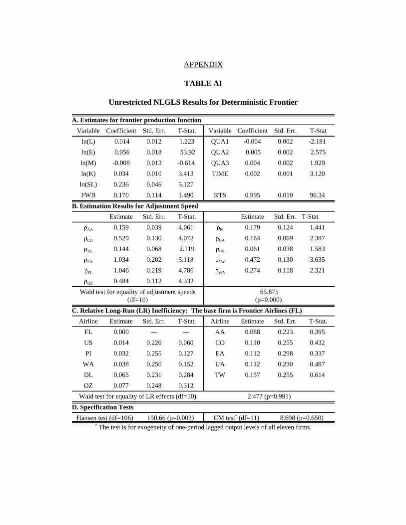
TABLE AI

Unrestricted NLGLS Results for Deterministic Frontier



ln(L) 0.014 0.012 1.223 QUA1 -0.004 0.002 -2.181

ln(E) 0.956 0.018 53.92 QUA2 0.005 0.002 2.575

ln(M) -0.008 0.013 -0.614 QUA3 0.004 0.002 1.929

ln(K) 0.034 0.010 3.413 TIME 0.002 0.001 3.120

ln(SL) 0.236 0.046 5.127

PWB 0.170 0.114 1.490 RTS 0.995 0.010 96.34


Estimate Std. Err. T-Stat. Estimate Std. Err. T-Stat

�AA 0.159 0.039 4.061 �PI 0.179 0.124 1.441

�CO 0.529 0.130 4.072 �UA 0.164 0.069 2.387

�DL 0.144 0.068 2.119 �US 0.061 0.038 1.583

�EA 1.034 0.202 5.118 �TW 0.472 0.130 3.635

�FL 1.046 0.219 4.786 �WA 0.274 0.118 2.321

�OZ 0.484 0.112 4.332

Wald test for equality of adjustment speeds(df=10)

65.875(p=0.000)

C. Relative Long-Run (LR) Inefficiency: The base firm is Frontier Airlines (FL)


FL 0.000 --- --- AA 0.088 0.223 0.395

US 0.014 0.226 0.060 CO 0.110 0.255 0.432

PI 0.032 0.255 0.127 EA 0.112 0.298 0.337

WA 0.038 0.250 0.152 UA 0.112 0.230 0.487

DL 0.065 0.231 0.284 TW 0.157 0.255 0.614

OZ 0.077 0.248 0.312


D. Specification Tests

Hansen test (df=106) 150.66 (p=0.003) CM test* (df=11) 8.698 (p=0.650)* The test is for exogeneity of one-period lagged output levels of all eleven firms.

TABLE AII

Unrestricted GMM2 Results for Stochastic Frontier



ln(L) 0.032 0.023 1.353 QUA1 -0.002 0.004 -0.639

ln(E) 0.914 0.062 14.64 QUA2 0.007 0.003 1.922

ln(M) 0.017 0.030 0.577 QUA3 0.005 0.003 1.722

ln(K) 0.064 0.051 1.253 TIME -0.0004 0.001 -0.265

ln(SL) 0.248 0.083 2.986

PWB 0.087 0.155 0.558 RTS 1.027 0.030 34.12


Estimate Std. Err. T-Stat. Estimate Std. Err. T-Stat

�AA 0.092 0.040 2.316 �PI 0.074 0.186 0.399

�CO 0.053 0.093 0.570 �UA 0.090 0.112 0.802

�DL 0.064 0.137 0.468 �US 0.044 0.042 1.031

�EA 0.030 0.213 0.142 �TWA 0.307 0.158 1.950

�FA 0.891 0.220 4.048 �WA 0.267 0.279 0.954

�OZ 0.233 0.149 1.568

Wald test for equality of adjustment speeds (df=10)

18.84(p=0.042)

C. Relative Long-Run (LR) Inefficiency: The base firm is Frontier Airlines (FL)


FL 0.000 --- --- EA 0.107 0.258 0.413

US 0.017 0.223 0.075 CO 0.117 0.238 0.490

WA 0.059 0.363 0.163 AA 0.128 0.223 0.574

DL 0.074 0.247 0.301 UA 0.149 0.242 0.615

PI 0.083 0.276 0.300 TW 0.177 0.278 0.639

OZ 0.099 0.262 0.375


D. Specification Tests


Documents

Estimation of Long-Run Inefficiency Levels: A Dynamic