Estimation of Heat Transfer to Flat Plates, Cones and Blunt Bodies

p.. e~ e¢3

z

/

MINISTRY OF T E C H N O L O G Y

AERONAUTICAL RESEARCH COUNCIL

REPORTS AND MEMORANDA

R. & M . No. 3637

Estimation of Heat Transfer to Flat Plates, Cones and Blunt Bodies

By

L. F. CRABTREE R. L. DOMMETT

and J. G. WOODLEY

R.A.E. Farnborough

LONDON: HER MAJESTY'S STATIONERY OFFICE

1970

PRICE £1 10s 0d [£1"50] NET

:Estimation of Heat Transfer to Flat and Blunt Bodies

By L. F. CRABTREE

R. L. DC)MMETT and

J. G. WOODLEY

R.A.E. Farnborough

Plates, Cones

Reports and Memoranda No. 3637" July, 1965

Summary. Section 1 gives some general concepts and definitions regarding heat transfer.

In Section 2 a method is described for calculating the rates of heat transfer to the surface of an ideal flat plate or sharp cone in an airstream at Mach numbers up to 10, for both laminar and fully turbulent boundary layers.

A system of predicting heat transfer to blunt-nosed bodies throughout the hypersonic speed range is given in Section 3, for laminar, transitional or turbulent boundary layers.

The methods were previously described in data sheets which included comparisons with classified experimental results. These experimental data have been excluded from the present report in order to publish it in an unclassified form.

It should be noted that no revision of the material presented has been done since 1962. Accordingly there may be parts of the report which have been out-dated to some extent by information published since that date.

Section 1.

1,3,

1.4.

Table 1

LIST OF CONTENTS

General Concepts of Aerodynamic Heating

1.1. Recovery factors and the 'intermediate enthalpy' method

1.2. Non-dimensional heat-transfer coefficients (Stanton and Nusselt numbers)

Reynolds analogy

The calculation of equilibrium temperature

Normal total emissivities of various substances

*Replaces R,A.E. Technical Report 65 137--A.R.C. 27 233.

.

.

Flat Plates and Cones up to M = l0 Excluding Dissociation Effects 2.1. Introduction

2.2. Laminar boundary layers

2.2.1. Flat plates

2.2.1.1. Local Stanton numbers

2.2.1.2. Mean Stanton numbers

2.2.2. Cones

2.3. Turbulent boundary layers

2.3.1. Flat plates

2.3.1.1. Local Stanton numbers

2.3.1.2. Mean Stanton numbers

2.3.2. Cones

2.4. Application : Computational procedures

2.4.1. Rapid approximate method

2.4.2. Complete method

Laminar boundary layers

Turbulent boundary layers

2.4.2.1.

2.4.2.2.

2.5. Comments

Heat Transfer to Blunt Bodies

3.1. Introduction

3.2. Methods of estimation

3.2.1. Laminar boundary layers

(a) Stagnation point

(b) Distribution around blunt body

(c) Total heat transfer

3.2.2. Turbulent boundary layers

3.2.3. Transition region

3.3. Application to particular eases

3.3.1. Laminar boundary layers

(a) Stagnation point

(b) Distribution around blunt body

3.3.2. Turbulent boundary layers

3.4. Discussion

3.5. Further comments

3.5.1. Swept cylinders

3.5.2.

3•5.3.

3.5.4.

3.5.5•

List of Symbols

References

General three-dimensional flow and bodies at incidence

Separated flow regimes

Wall cat~ytic efficiency

Radiation from gas cap

Illustrations--Figs. 1 to 17

Detachable Abstract Cards

1. General Concepts of Aerodynamic Heating. (Note :--The appropriate units for dimensional quantities used in the following analysis are indicated

in the list of symbols.) l

1.1. Recovery Factors and the 'Intermediate Enthalpy' Method. The rate of convective heat transfer per unit area to or from a surface in an airstream of velocity u

and density p is given by

q = h(i,-iw) (1.1)

T

where i = f cp dT is the enthalpy of the air (cp being the specific heat of air at constant pressure) and h is

o the heat-transfer factor .

The subscript w denotes conditions at the wall (body surface) and subscript r denotes recovery conditions at the wall, i.e. for zero heat transfer•

The wall enthalpy for zero heat transfer (or recovery enthalpy) is given by

ru~ i, = ie-t 2J (1.2)

where subscript e refers to local conditions at the edge of the boundary layer, r is an enthalpy recovery factor and J is the mechanical equivalent of heat. This equation should be compared with the expression for total or stagnation enthalpy

2 • U e

1"It should be noted that h is a dimensional quantity. Non-dimensional heat transfer coefficients are also often used (see Section 1.2) but h is more convenient for some applications. In particular, it will transpire in Section 2.2.1 that a convenient way of presenting heat transfer data for flat plates and cones is to plot graphs of the quantity hx (where x denotes distance along the surface) against the Reynolds number Re* corresponding to 'intermediate' enthalpy i* as variable parameter.

which for constant cp takes the form

v-= 1+ M 2 . Ie

Similarl\. t\w con~,t~nt or,. equation [1.21 may be w/']tten as

ir l + r ~ . } _ M 2 . ie

(1.2a)

Eckert 1 and Monaghan 2 have shownt that, for a wide range of Mach numbers and temperatures, a close approximation is obtained for the heat transfer to an ideal fiat plate in both laminar and fully turbulent flow if the physical properties of air appearing in the incompressible flow formulae are evaluated at a temperature corresponding to an 'intermediate' enthalpy i* given by the simple formula

i* = i e + 0.5 (iw - ie) + 0"22 (i r -- ie) (1.3)

which, in virtue of (1.2a) may be written in the form

i* f i '~- !e + 0"22"~ ~--~ M2 - = 1+ 0.5 r . ie Ir--I e J

(1.3a)

Usually ie and iw will be known and i, is given by equation (1.2) with, for laminar boundary layers

r -"- (Pr*) "~ (1.4)

which is the Pohlhausen formula with Prandtl number (see Section 1.2 below) evaluated at the temperature T* corresponding to i*.

For turbulent boundary layers

r = 0-89 (1.5)

which is a mean of experimental values; a good approximation to these is also given by Squire's semi- empirical result that r = (Pr) 1/3.

The intermediate enthalpy method can also be applied to the cylindrical parts of bodies of revolution at zero angle of attack, and to sharp cones (a) by use of a simple transformation of co-ordinates introduced by Mangler for the laminar case, and (b) by other theoretical considerations due to Young and to van Driest for the turbulent case. The cone results are discussed in Section 2.3.2.

It has also been found that the intermediate enthalpy method gives useful results in cases where pressure gradients exist, provided that true local conditions are used in the formulae (see for example Refs. 7 and 8}.

1.2 Non-Dimens io ,a l Heat -Trans fer Coefficients (Stanton amt Nussel t Nm~Ther.s).

The heat transfer factor h in equation (l.1) is dimensional and it varies considerably with flight conditions, so in aerodynamic calculations it is often more convenient to work with the non-dimensional heat-transfer coefficient or Stanton number St, defined by

h St = Pe Ue (1.6)

tFo r a fuller discussion see E. L. Knuth 'Use of reference states and constant property solutions in predicting mass, momentum and energy-transfer rates in high speed laminar flows'. Int. J. o f Hea t and Mass Transfer. Vol. 6, No. 1, p. 1. January 1963.

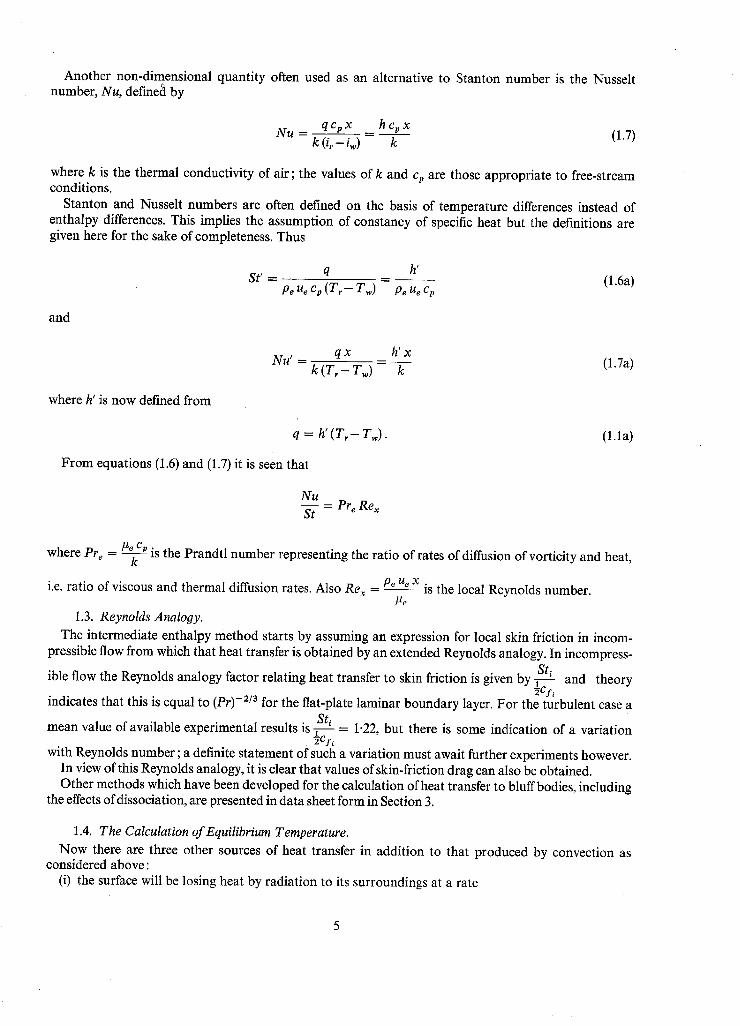
Another non-dimensional quantity often used as an alternative to Stanton number is the Nusselt number, Nu, definea by

N u = q c p x = h c p x k (¢ - i~) k (1.7)

where k is the thermal conductivity of air; the values of k and cp are those appropriate to free-stream conditions.

Stanton and Nusselt numbers are often defined on the basis of temperature differences instead of enthalpy differences. This implies the assumption of constancy of specific heat but the definitions are given here for the sake of completeness. Thus

St' = q h' - - - ( 1 . 6 a ) p~ u~ cp ( T , - T,o) pe ue cp

and

Nu' - q x h' x

k (T r - Tw) - k (1.7a)

where h' is now defined from

q = h ' ( T r - T w ) .

From equations (1.6) and (1.7) it is seen that

(1.1a)

Nu St = Pr~ Re x

where Pr e - #~ cp is the Prandtl number representing the ratio of rates of diffusion of vorticity and heat, k

i.e. ratio of viscous and thermal diffusion rates. Also Rex - Pe u~ x is the local Reynolds number. kt~

1.3. Reynolds Analogy.

The intermediate enthalpy method starts by assuming an expression for local skin friction in incompressible flow from which that heat transfer is obtained by an extended Reynolds analogy. In incompress-

Sti ible flow the Reynolds analogy factor relating heat transfer to skin friction is given by ½cl, and theory

indicates that this is equal to (Pr)-2/a for the flat-plate laminar boundary layer. For the turbulent case a

mean value of available experimental results is Sh ½c f, = 1.22, but there is some indication of a variation

with Reynolds number; a definite statement of such a variation must await further experiments however. In view of this Reynolds analogy, it is clear that values of skin-friction drag can also be obtained. Other methods which have been developed for the calculation of heat transfer to bluff bodies, including

the effects of dissociation, are presented in data sheet form in Section 3.

1.4. The Calculation of Equilibrium Temperature.

Now there are three other sources of heat transfer in addition to that produced by convection as considered above:

(i) the surface will be losing heat by radiation to its surroundings at a rate

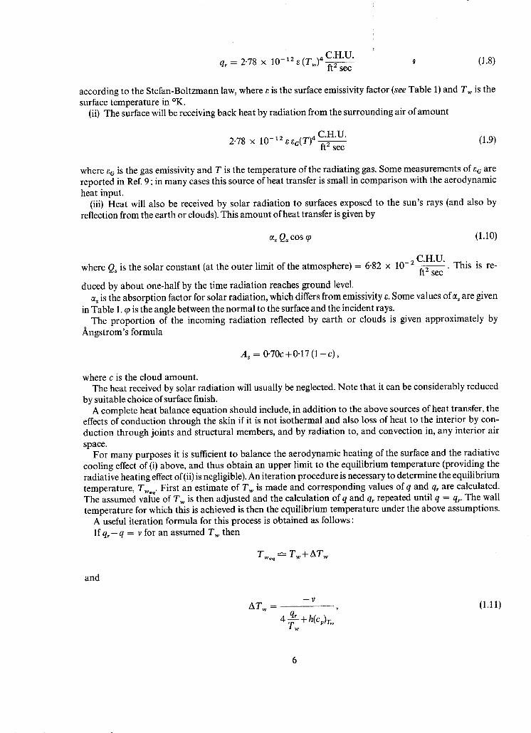
q, = 2"78 x 10-12e(T~) 4C'H'U" ft 2 sec

(1.8)

according to the Stefan-Boltzmann law, where e is the surface emissivity factor (see Table 1) and Tw is the surface temperature in °K.

(ii) The surface will be receiving back heat by radiation from the surrounding air of amount

2"78 x 10 - 1 2 eeG(T) 4 C.H.U. ft 2 sec

(1.9)

where so is the gas emissivity and T is the temperature of the radiating gas. Some measurements of e~ are reported in Ref. 9; in many cases this source of heat transfer is small in comparison with the aerodynamic heat input.

(iii) Heat will also be received by solar radiation to surfaces exposed to the sun's rays (and also by reflection from the earth or clouds). This amount of heat transfer is given by

a~ Qs cos tO (1.10)

where Q~ is the solar constant (at the outer limit of the atmosphere) = 6.82 × 10- 2 C.H.U. This is re- fE E sec "

duced by about one-half by the time radiation reaches ground level. cq is the absorption factor for solar radiation, which differs from emissivity e. Some values of ~s are given

in Table 1. ~ is the angle between the normal to the surface and the incident rays. The proportion of the incoming radiation reflected by earth or clouds is given approximately by

Angstrom's formula

As = 0-70c+0-17 (1 - c ) ,

where c is the cloud amount. The heat received by solar radiation will usually be neglected. Note that it can be considerably reduced

by suitable choice of surface finish. A complete heat balance equation should include, in addition to the above sources of heat transfer, the

effects of conduction through the skin if it is not isothermal and also loss of heat to the interior by conduction through joints and structural members, and by radiation to, and convection in, any interior air space.

For many purposes it is sufficient to balance the aerodynamic heating of the surface and the radiative cooling effect of (i) above, and thus obtain an upper limit to the equilibrium temperature (providing the radiative heating effect of(ii) is negligible). An iteration procedure is necessary to determine the equilibrium temperature, T~e q. First an estimate of Tw is made and corresponding values of q and q, are calculated. The assumed value of Tw is then adjusted and the calculation of q and qr repeated until q = qr. The wall temperature for which this is achieved is then the equilibrium temperature under the above assumptions.

A useful iteration formula for this process is obtained as follows : If q , - q = v for an assumed T~ then

T~o ~ ~ T~, + ATw

and

n ~ AT w = , (1.11)

4 q ~ + rw h(cp)r~

where h is the heat transfer factor and (Cp)rw is the specific heat of air at constant pressure, evaluated at the assumed wall temperature, Tw.

Throughout the calculations in this report the standard atmospheric data used are those of Ref. 3.

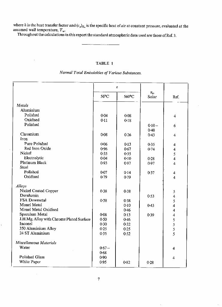
TABLE 1

Normal Total Emissivities of Various Substances.

Metals Aluminium

Polished Oxidised Polished

Chromium Iron

Pure Polished Red Iron Oxide

Nickel Electrolytic

Platinum Black Steel

Polished Oxidised

Alloys Nickel Coated Copper Duralumin FSA Dowmetal Monel Metal Monel Metal Oxidised Speculum Metal J.H.Mg. Alloy with Chrome Plated Surface Inconel 350 Aluminium Alloy 24 ST Aluminium

Miscellaneous Materials Water

Polished Glass White Paper

56°C

0"04 0"11

0'08

0.06 0.96 0-35 0.04 0.93

0.07 0.79

0.38

0.38

0.08 0-50 0-30 0-25 0.35

0"67 - 0.68 0.90 0.95

560°C

0.08 0.18

0.26

0.13 0.67 0.35 0.10 0.97

0.14 0.79

0.38

0.38 0-10 0.46 0.13 0.46 0.32 0.25 0.32

0.82

Solar

0.10- 0.40 0.43

0.35 0.74

0-28 0.97

0.37

0.53

0.43

0.39

0-28

Ref.

4 4

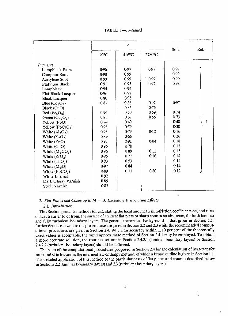
TABLE 1--continued

Pigments Lampblack Paint Camphor Soot Acetylene Soot Platinum Black Lampblack Flat Black Lacquer Black Lacquer Blue (C0203) Black (CuO)

Red (Fe2Oa) Green (Cu203) Yellow (PbO) Yellow (PbCrO4) White (A1203) White (Y203) White (ZnO) White (CnO) White (MgCO3) White (ZrO2) White (ThO2) White (MgO) White (PbCO3) White Enamel Dark Glossy Varnish Spirit Varnish

70°C

0"96 0"98 0"99 0"91

416°C

0"97 0"99 0"99 0"95

2780°C

0"97

0"99 0"97

Solar

0"97 0"99 0"99 0"98

Ref.

0.94 0-94 0.96 0-98 0"80 0'95 0.87 0"86

0'85 0"96 0"70 0"95 0-67 0"74 0"49 0.95 0"59 0"98 0'79 0"89 0"66 0"97 0"91 0"96 0"78 0"96 0"89 0"95 0"77 0"93 0'53 0"97 0"84 0"89 0"71 0"92 0"89 0"83

0.97 0"97 0-76 0-59 0"74 0"55 0"73

0-48 0"30

0"12 0"16 0'26

0"04 0"18 0'15

0"11 0"15 0"16 0"14

0"14 0"14

0"80 0"12

2. Flat Plates and Cones up to M = 10 Excluding Dissociation Effects.

2.1. Introduction. This Section presents methods for calculating the local and mean skin-friction coefficients on, and rates

of heat transfer to or from, the surface of an ideal flat plate or sharp cone in an airstream, for both laminar and fully turbulent boundary layers. The general theoretical background is that given in Section 1.1; further details relevant to the present case are given in Section 2.2 and ,2.3 while the recommended computational procedures are given in Section 2.4. Where an accuracy within _ 10 per cent of the theoretically exact values is acceptable, the rapid approximate method of Section 2.4.1 may be employed. To obtain a more accurate solution, the routines set out in Section 2.4.2.1 (laminar boundary layers) or Section 2.4.2.2 (turbulent boundary layers) should be followed.

The basis of the computational procedures proposed in Section 2.4 for the calculation of heat-transfer rates and skin friction is the intermediate enthalpy method, of which a broad outline is given in Section 1.1. The detailed application of this method to the particular cases of flat plates and cones is described below in Sections 2.2 (laminar boundary layers) and 2.3 (turbulent boundary layers).

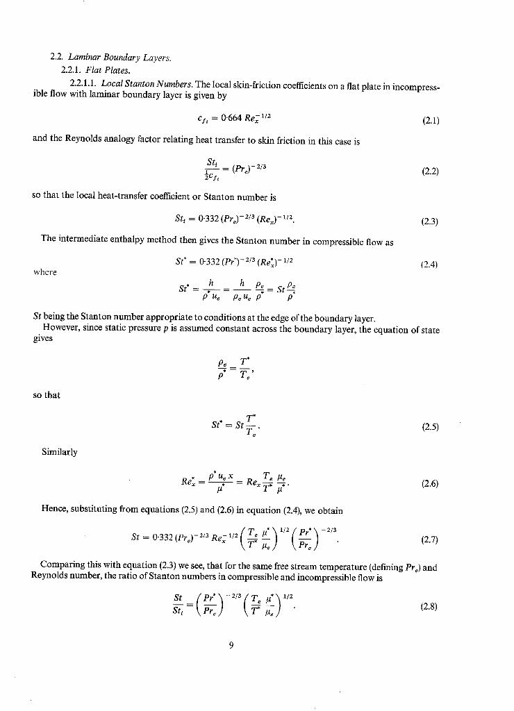
2.2. Laminar Boundary Layers.

2.2.1. Flat Plates.

2.2.1.1. Local Stanton Numbers. The local skin-friction coefficients on a flat plate in incompress- • ible flow with laminar boundary layer is given by

cy, = 0"664 Re; 1/2

and the Reynolds analogy factor relating heat transfer to skin friction in this case is

(2.1)

Sti (Pre)- 2/a 1 -~C f i

SO that the local heat-transfer coefficient or Stanton number is

(2.2)

Sti = 0"332 (Pre)-2/3 (Rex)- 1/2. (2.3)

The intermediate enthalpy method then gives the Stanton number in compressible flow as

St* = 0-332 (Pr*)- 2/3 (Re*)- 1/2 (2.4) where

st" = ,h = __h _P = s t P Ue Pe U~ p p

St being the Stanton number appropriate to conditions at the edge of the boundary layer. However, since static pressure p is assumed constant across the boundary layer, the equation of state

gives

P 4 _ T * p T~'

so that

T* St* = S t - - . (2.5)

Te

Similarly

, p*UeX T~ Ig~ Rex = It* -- Rex T, " (2.6)

It

Hence, substituting from equations (2.5) and (2.6) in equation (2.4), we obtain

St = 0"332 (Pre)- 2/3 Re ; 1/2 \ Pre]

(2.7)

Comparing this with equation (2.3) we see, that for the same free stream temperature (defining Pre) and Reynolds number, the ratio of Stanton numbers in compressible and incompressible flow is

Sti \ Pre } Pc} " (2.8)

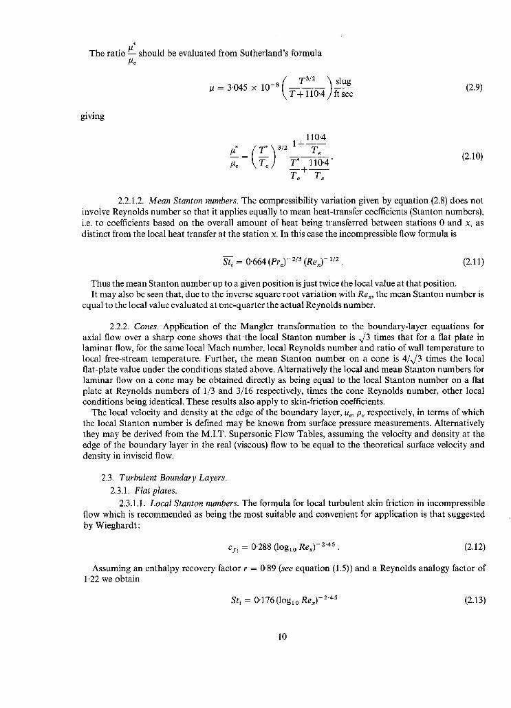
The ratio - - should be evaluated from Sutherland's formula

T a/z ) slug # = 3.045 x 10- s \ T-7- ]-i-0.4 ft sec (2.9)

giving

110.4

#e Te T* 110"4" Te Te

(2.10)

2.2.1.2. Mean Stanton numbers. The compressibility variation given by equation (2.8) does not involve Reynolds number so that it applies equally to mean heat-transfer coefficients (Stanton numbers), i.e. to coefficients based on the overall amount of heat being transferred between stations 0 and x, as distinct from the local heat transfer at the station x. In this case the incompressible flow formula is

St---~ = 0"664 (Pre)-2/3 (Rex)- 1/2. (2.11)

Thus the mean Stanton number up to a given position is just twice the local value at that position. It may also be seen that, due to the inverse square root variation with Rex, the mean Stanton number is

equal to the local value evaluated at one-quarter the actual Reynolds number.

2.2.2. Cones. Application of the Mangler transformation to the boundary-layer equations for axial flow over a sharp cone shows that the local Stanton number is ~/3 times that for a flat plate in laminar flow, for the same local Mach number, local Reynolds number and ratio of wall temperature to local free-stream temperature. Further, the mean Stanton number on a cone is 4/n/3 times the local flat-plate value under the conditions stated above. Alternatively the local and mean Stanton numbers for laminar flow on a cone may be obtained directly as being equal to the local Stanton number on a flat plate at Reynolds numbers of 1/3 and 3/16 respectively, times the cone Reynolds number, other local conditions being identical. These results also apply to skin-friction coefficients.

The local velocity and density at the edge of the boundary layer, ue, Pe respectively, in terms of which the local Stanton number is defined may be known from surface pressure measurements. Alternatively they may be derived from the M.I.T. Supersonic Flow Tables, assuming the velocity and density at the edge of the boundary layer in the real (viscous) flow to be equal to the theoretical surface velocity and density in inviscid flow.

2.3. Turbulent Boundary Layers. 2.3.1. Flat plates.

2.3.1.1. Local Stanton numbers. The formula for local turbulent skin friction in incompressible flow which is recommended as being the most suitable and convenient for application is that suggested by Wieghardt:

cy, = 0"288 (loglo Rex) -2'45 • (2.12)

Assuming an enthalpy recovery factor r = 0'89 (see equation (1.5)) and a Reynolds analogy factor of 1-22 we obtain

Sti = 0-176 (logto Rex)- 2.4s (2.13)

10

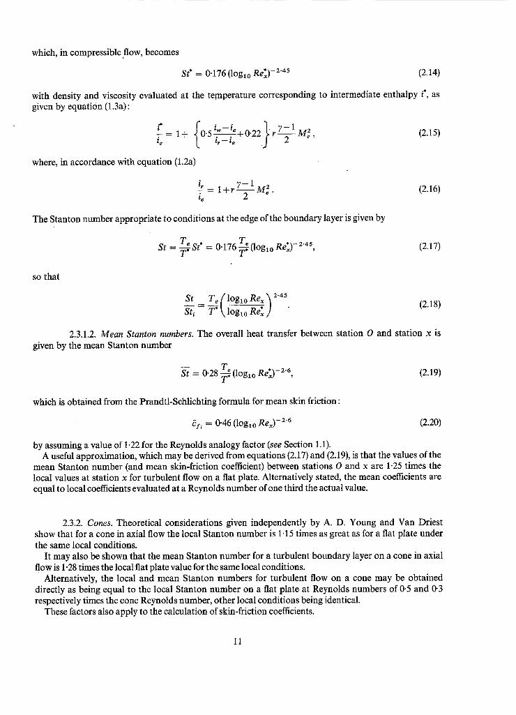
which, in compressible flow, becomes

St* = 0.176 (loglo Re~) -2"4s (2.14)

with density and viscosity evaluated at the temperature corresponding to intermediate enthalpy i*, as given by equation (1.3a):

i* / " -- " - - : 1+ l 0"51~w" ;e - ' [ -0"22~r~--~M2' ie "r- "e i j

where, in accordance with equation (1.2a)

(2.15)

7-= l + r M~. (2.16) le

The Stanton number appropriate to conditions at the edge of the boundary layer is given by

r e . St = ~ St = 0"176 (loglo Re*)-2"45, (2.17)

so that

S_.t_t Te { 1Oglo Rex ~ 2.45

Sti = T* \ loglo Re~ ] " (2.18)

2.3.1.2. Mean Stanton numbers. The overall heat transfer between station 0 and station x is given by the mean Stanton number

Te R * 26 = 0"28 ~-~ (loglo e~)- " , (2.19)

which is obtained from the Prandtl-Schlichting formula for mean skin friction :

6y, = 0"46 (loglo Rex) -2"6 (2.20)

by assuming a value of 1.22 for the Reynolds analogy factor (see Section 1.1). A useful approximation, which may be derived from equations (2.17) and (2.19), is that the values of the

mean Stanton number (and mean skin-friction coefficient) between stations O and x are 1.25 times the local values at station x for turbulent flow on a flat plate. Alternatively stated, the mean coefficients are equal to local coefficients evaluated at a Reynolds number of one third the actual value.

2.3.2. Cones. Theoretical considerations given independently by A. D. Young and Van Driest show that for a cone in axial flow the local Stanton number is 1.15 times as great as for a flat plate under the same local conditions.

It may also be shown that the mean Stanton number for a turbulent boundary layer on a cone in axial flow is 1.28 times the local flat plate value for the same local conditions.

Alternatively, the local and mean Stanton numbers for turbulent flow on a cone may be obtained directly as being equal to the local Stanton number on a flat plate at Reynolds numbers of 0-5 and 0.3 respectively times the cone Reynolds number, other local conditions being identical.

These factors also apply to the calculation of skin-friction coefficients.

i1

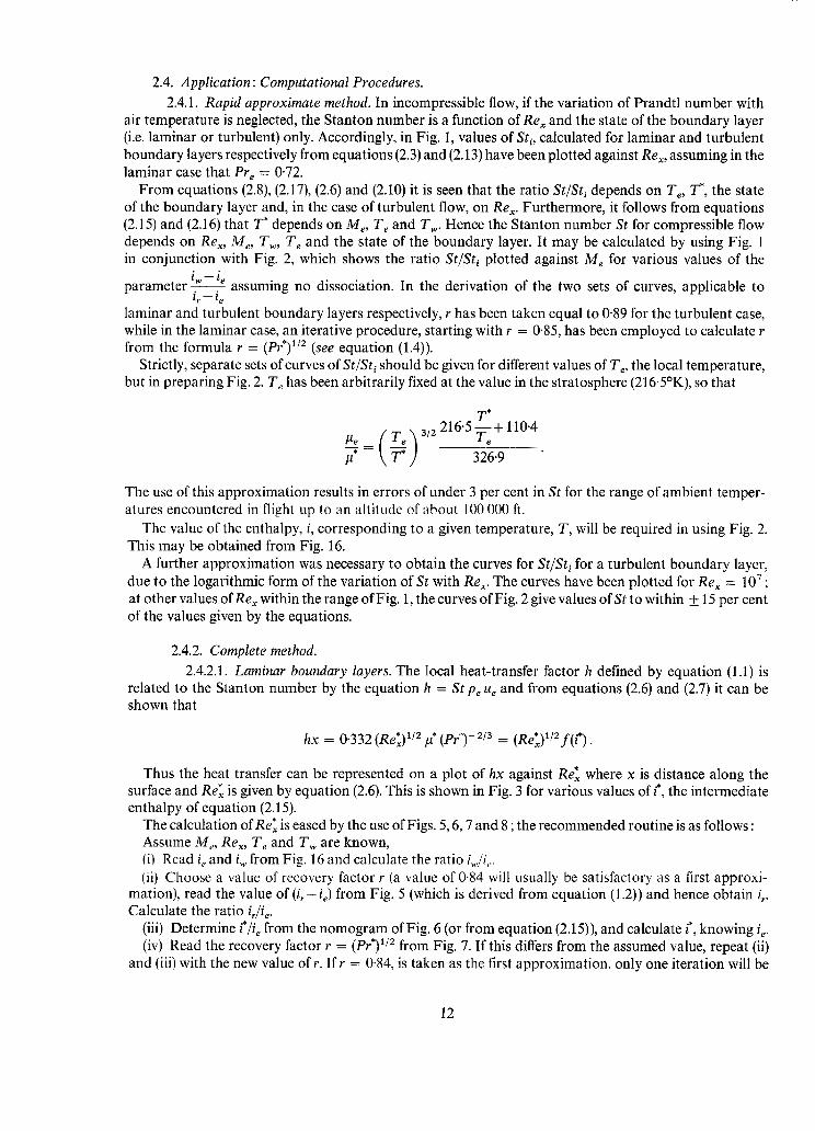
2.4. Application: Computational Procedures. 2.4.1. Rapid approximate method. In incompressible flow, if the variation of Prandtl number with

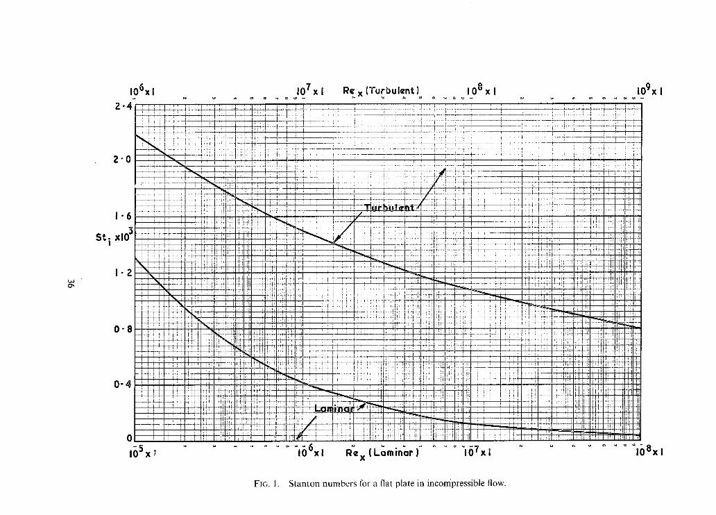
air temperature is neglected, the Stanton number is a function of Rex and the state of the boundary layer (i.e. laminar or turbulent) only. Accordingly, in Fig. 1, values of Sty, calculated for laminar and turbulent boundary layers respectively from equations (2.3) and (2.13) have been plotted against Rex, assuming in the laminar case that Pre = 0"72.

From equations (2.8), (2.17), (2.6) and (2.10) it is seen that the ratio St/Sti depends on Te, T*, the state of the boundary layer and, in the case of turbulent flow, on Rex. Furthermore, it follows from equations (2.15) and (2.16) that T* depends on Me, Te and Tw. Hence the Stanton number St for compressible flow depends on Rex, Me, Tw, Te and the state of the boundary layer. It may be calculated by using Fig. 1 in conjunction with Fig. 2, which shows the ratio St/St~ plotted against M e for various values of the

parameter iw-. .ie assuming no dissociation. In the derivation of the two sets of curves, applicable to I r - - I e

laminar and turbulent boundary layers respectively, r has been taken equal to 0-89 for the turbulent case, while in the laminar case, an iterative procedure, starting with r = 0.85, has been employed to calculate r from the formula r = (Pr*) 1/z (see equation (1.4)).

Strictly, separate sets of curves of St/St~ should be given for different values of T e, the local temperature, but in preparing Fig. 2, Te has been arbitrarily fixed at the value in the stratosphere (216.5°K), so that

T*

( )3122 65 +,104 326.9 The use of this approximation results in errors of under 3 per cent in St for the range of ambient temperatures encountered in flight up to an altitude of about 100 000 ft.

The value of the enthalpy, i, corresponding to a given temperature, T, will be required in using Fig. 2. This may be obtained from Fig. 16.

A further approximation was necessary to obtain the curves for St/Sti for a turbulent boundary layer, due to the logarithmic form of the variation of St with Rex. The curves have been plotted for Rex = 107; at other values of Rex within the range of Fig. 1, the curves of Fig. 2 give values of St to within _+ 15 per cent of the values given by the equations.

2.4.2. Complete method. 2.4.2.1. Laminar boundary layers. The local heat-transfer factor h defined by equation (1.1) is

related to the Stanton number by the equation h -- St Pe Ue and from equations (2.6) and (2.7) it can be shown that

hx = 0.332 (Re*) 1/2 #* (Pr*)- 2/3 = (Re*x)l/2 f(i*).

Thus the heat transfer can be represented on a plot of hx against Re* where x is distance along the surface and Re* is given by equation (2.6). This is shown in Fig. 3 for various values of/*, the intermediate enthalpy of equation (2.15).

The calculation of Re*~ is eased by the use of Figs. 5, 6, 7 and 8 ; the recommended routine is as follows : Assume Me, Rex, Te and T w are known, (il Read ie and i,. from Fig. 16 and calculate the ratio iw/i,.. (ii) Choose a value of recovery factor r (a value of 0-84 will usually be satisfactory as a first approxi-

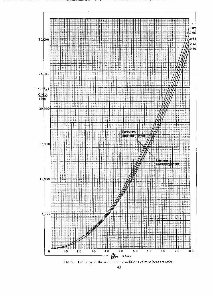
mation), read the value of (i~-ie) from Fig. 5 (which is derived from equation (1.2)) and hence obtain it. Calculate the ratio ir/i e.

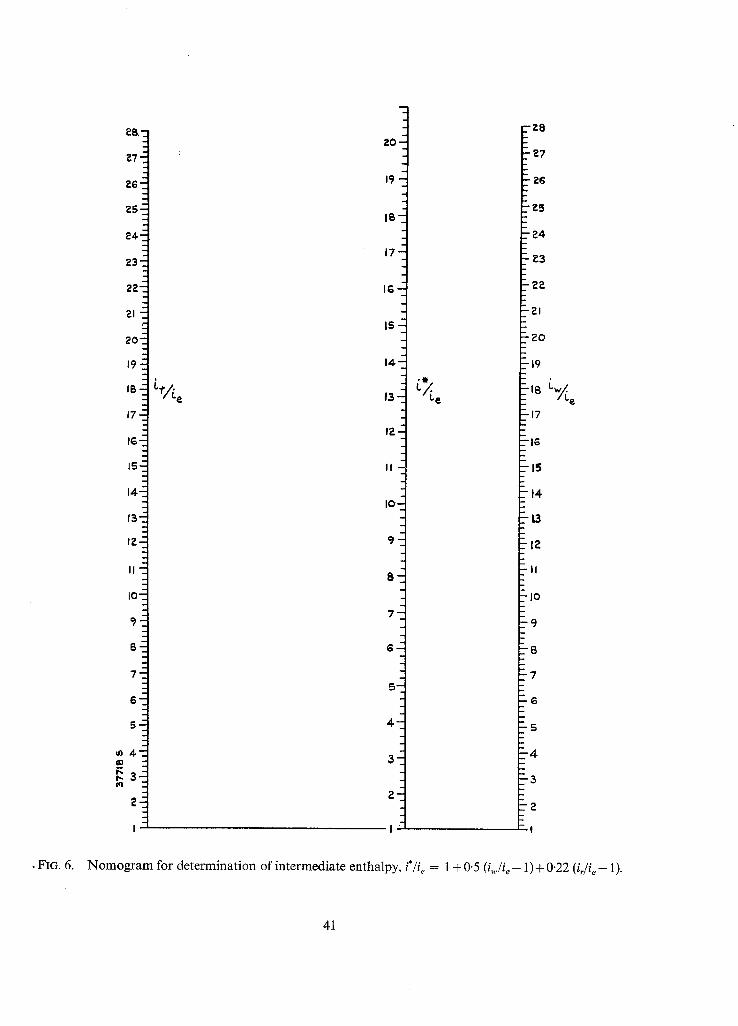
(iii) Determine {~/ie from the nomogram of Fig. 6 (or from equation (2.15)), and calculate i*, knowing ie. (iv) Read the recovery factor r = (Pr*) 1/2 from Fig. 7. If this differs from the assumed value, repeat (ii)

and (iii) with the new value oft . I f r = 0.84, is taken as the first approximation, only one iteration will be

12

necessary in most cases.

(v) Read the ratio Rex/Re*~ from Fig. 8 (equation (2.6)) and using the known value of Rex = pe ue X,

calculate Re*. #~ (vi) Tile local heat-transfer factor h may now be obtained from the plot of hx ~ Re*~ in Fig. 3 and the

heat-transfer rate calculated from the equation q = h ( i , - iw) (equation (1.1)). (vii) To obtain the local skin-friction coefficient, first calculate the local Stanton number from the

equation

h S t -

Pe Ue

St = (Pr*)-2/a, from Fig. 7 knowing i*, and calculate c:. then determine the Reynolds analogy factor, ~cf

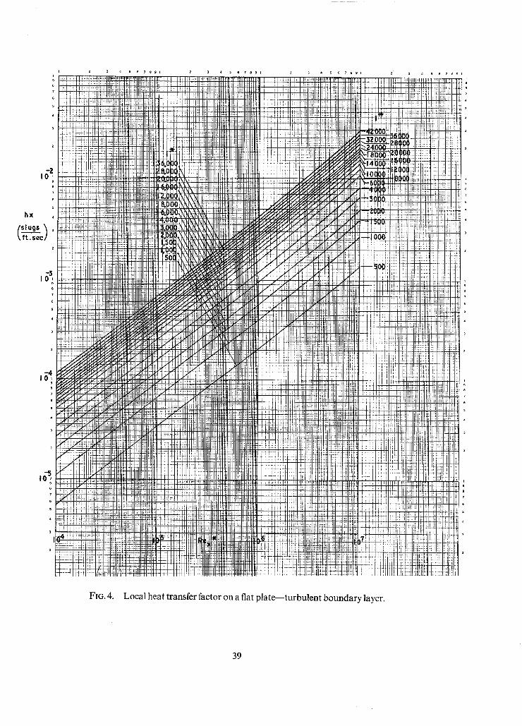
2.4.2.2. Turbulent boundary layers. Using the relationship h = St peU e in conjunction with equations (2.3), (2.5), (2.6) and (2.14), it can be shown that

hx = 0"176 (loglo Re*~) -2"45 It* Re*

so that the heat transfer can again be represented by curves of hx against Re* with i* as a parameter (see Fig. 4). The procedure for calculating Re* is however much simpler since the recovery factor r for a turbulent boundary layer on a flat plate is taken to be constant at r = 0"89 :

(i) Read ie and iw from Fig. 16 and calculate the ratio i~/i,. (ii) Read the value o f ( i , - ie) from the curve labelled r = 0.89 on Fig. 5 which is derived from equation

(1.2) and hence obtain it. Calculate the ratio i,/ie. (iii) Determine i*/ie from the nomogram of Fig. 6 or from equation (2.15) and calculate i*, knowing i e.

(iv) Read the value of the ratio Re=/Re* from Fig. 8 (equation (2.6)) and calculate Re*, knowing Rex. (v) The local heat-transfer factor h may now be obtained from the curves o f hx ,,~ Re* in Fig. 4 for the

appropriate value of i*. The heat-transfer rate is again calculated from the equation

q = h (i r - iw).

(vi) To obtain the local skin-friction coefficient, first calculate the local Stanton number from the equation St = h/pe ue. Then since the Reynolds analogy factor is assumed constant,

St ½ c:

- 1 . 2 2

the value of c: may be calculated.

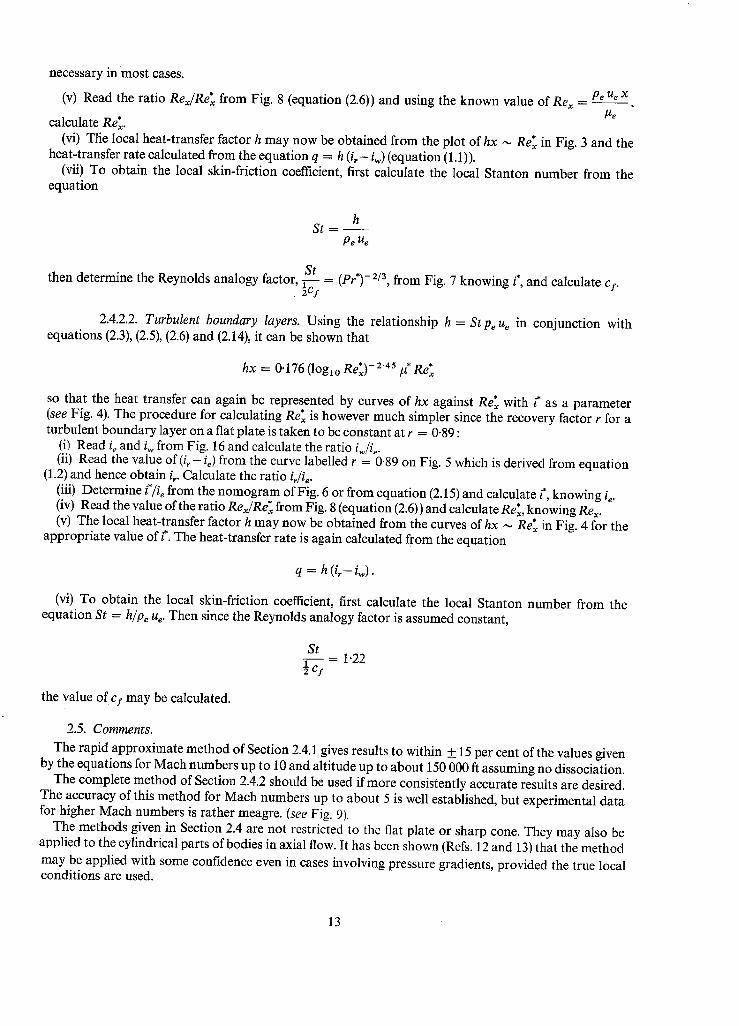
2.5. Comments.

The rapid approximate method of Section 2.4.1 gives results to within _+ 15 per cent of the values given by the equations for Mach numbers up to 10 and altitude up to about 150 000 ft assuming no dissociation.

The complete method of Section 2.4.2 should be used if more consistently accurate results are desired. The accuracy of this method for Mach numbers up to about 5 is well established, but experimental data for higher Mach numbers is rather meagre. (see Fig. 9).

The methods given in Section 2.4 are not restricted to the flat plate or sharp cone. They may also be applied to the cylindrical parts of bodies in axial flow. It has been shown (Refs. 12 and 13) that the method may be applied with some confidence even in cases involving pressure gradients, provided the true local conditions are used.

13

The results of Section 2.4 apply only to smooth surfaces. Roughness can cause appreciable increases in heat transfer and skin friction and it is also important in accelerating transition to turbulence.

All of the methods and results given above are for the special case of an isothermal wall. Various schemes have been proposed for calculating heat transfer when longitudinal surface temperature gradients are present, but all involve a fair degree of computational effort.

Particular reference may be made to the work of Eckert et a114'1s wherein details of earlier work by other investigators is quoted. The method of Spalding 16 is perhaps somewhat simpler.

3. Heat Transfer to Blunt Bodies. 3.1. Introduction.

This Section describes methods of predicting heat transfer from laminar or turbulent boundary layers applicable to blunt-nosed bodies at hypersonic speeds. Formulae are given for the stagnation point heating and for the distribution of heating from laminar and turbulent boundary layers over blunt nosed two dimensional and axisymmetric bodies at zero incidence which are valid for air in dissociation equilibrium. A knowledge of the flow properties, pressure, velocity and temperature at the outer edge of the boundary layer and of the thermodynamic and transport properties of air is assumed.

The possible effects arising from frozen flow with catalytic recombination at the wall are discussed. Other chemical reactions, with the wall material or in the boundary layer, transpiration and interaction with ablating surfaces are ignored.

The possible application of the method of this section to more general three dimensional flows, such as occur over a body at incidence, is considered.

In general it is impossible to reduce the methods to a series of graphs but design charts are provided for stagnation point heating and for the distribution of laminar boundary-layer heating over hemisphere- cylinders and spherically-capped-cone combinations.

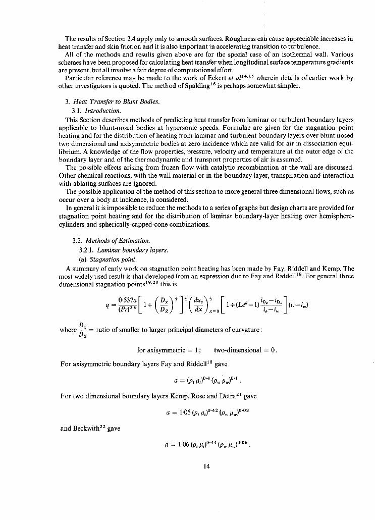
3.2. Methods of Estimation. 3.2.1. Laminar boundary layers. (a) Stagnation point.

A summary of early work on stagnation point heating has been made by Fay, Riddell and Kemp. The most widely used result is that developed from an expression due to Fay and Riddell 1 s. For general three dimensional stagnation points 19,z o this is

=0"537a F D ~ ~ &fdue~ ~ [l+(Le,~ 1)iD,,-i~](i,._i~) where D~ = ratio of smaller to larger princilial diameters of curvature :

for axisymmetric = I ; two-dimensional = 0.

For axisymmetric boundary layers Fay and Riddell is gave

a = (p,/h) °'4 (Pw #w) °' 1.

For two dimensional boundary layers Kemp, Rose and Detra 21 gave

a = 1.05 (Pt #t) °'42 (P~ #w) °'°s

and Beckwith 22 gave

a = 1.06 (Pt #,)0.44 (Pw #,~)o.o6.

14

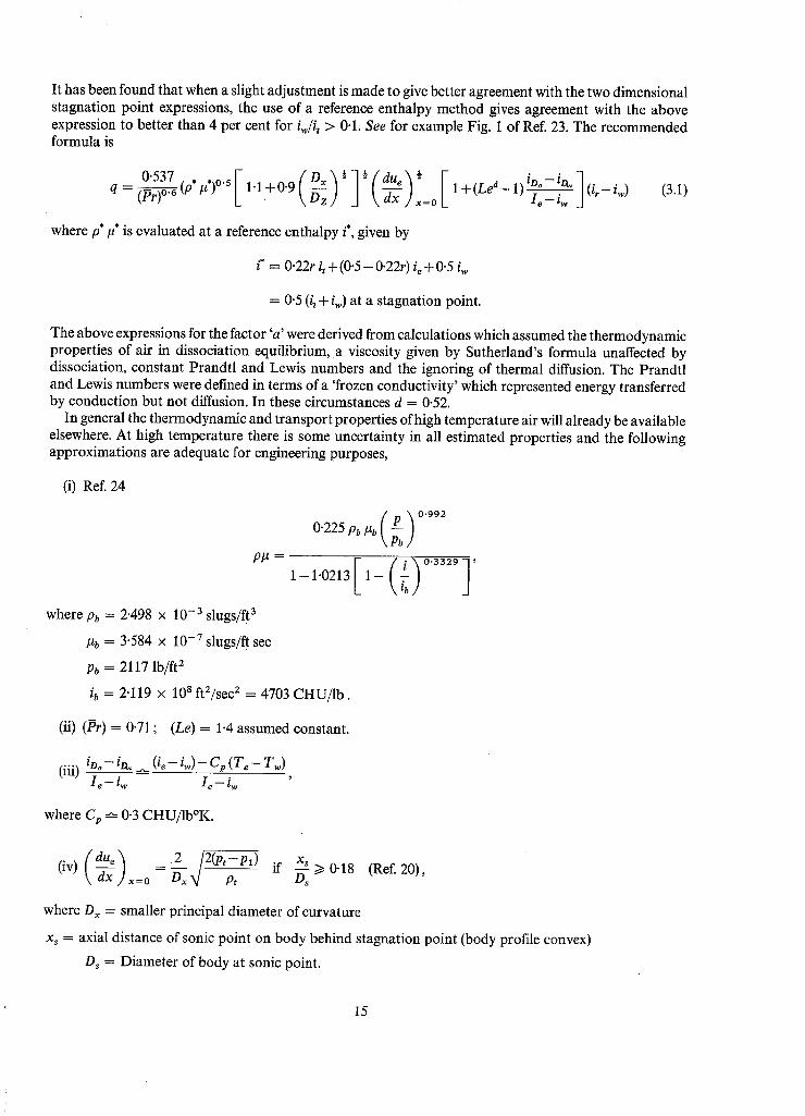
It has been found that when a slight adjustment is made to give better agreement with the two dimensional stagnation point expressions, the use of a reference enthalpy method gives agreement with the above expression to better than 4 per cent for iw/it > 0.1. See for example Fig. 1 of Ref. 23. The recommended formula is

E ,oi 0"537 ½ ~(due ) ½ ~l+(Le-1)--v----z-- . ] ( i r - i~) q = ~ ( p * # * ) o . 5 1-1.+0.9 \~x,/x=o L . e - r . , _1

where p* ~t* is evaluated at a reference enthalpy i*, given by

(3.1)

i* = 0.22r it + (0.5 - 0.22r) ie + 0.5 iw

= 0.5 (it+ iw) at a stagnation point.

The above expressions for the factor 'a' were derived from calculations which assumed the thermodynamic properties of air in dissociation equilibrium, a viscosity given by Sutherland's formula unaffected by dissociation, constant Prandtl and Lewis numbers and the ignoring of thermal diffusion. The Prandtl and Lewis numbers were defined in terms of a 'frozen conductivity' which represented energy transferred by conduction but not diffusion. In these circumstances d = 0.52.

In general the thermodynamic and transport properties of high temperature air will already be available elsewhere. At high temperature there is some uncertainty in all estimated properties and the following approximations are adequate for engineering purposes,

(i) Ref. 24

p # =

where Pb = 2"498 X 10 -3 slugs/ft 3

#b = 3"584 X 10 -7 slugs/ft sec

Pb = 2117 lb/ft 2

i ~ 0.3329

i b = 2"119 x 10 s ft2/sec 2 = 4703 CHU/Ib.

(ii) (Pr) = 0.71 ; (Le) = 1.4 assumed constant.

(iii) ioo- i1~, ~ (ie- i~,)- Cp (T e - Tw) I e - iw I e - - i w

where C v -"- 0"3 CHU/Ib°K.

{ due ) 2 ~ x~ (iv) \-d--~x ] , = o = ~-xN / ~-t if ~ i> 0.18 (Ref. 20),

where D x = smaller principal diameter of curvature

xs = axial distance of sonic point on body behind stagnation point (body profile convex)

D~ = Diameter of body at sonic point.

15

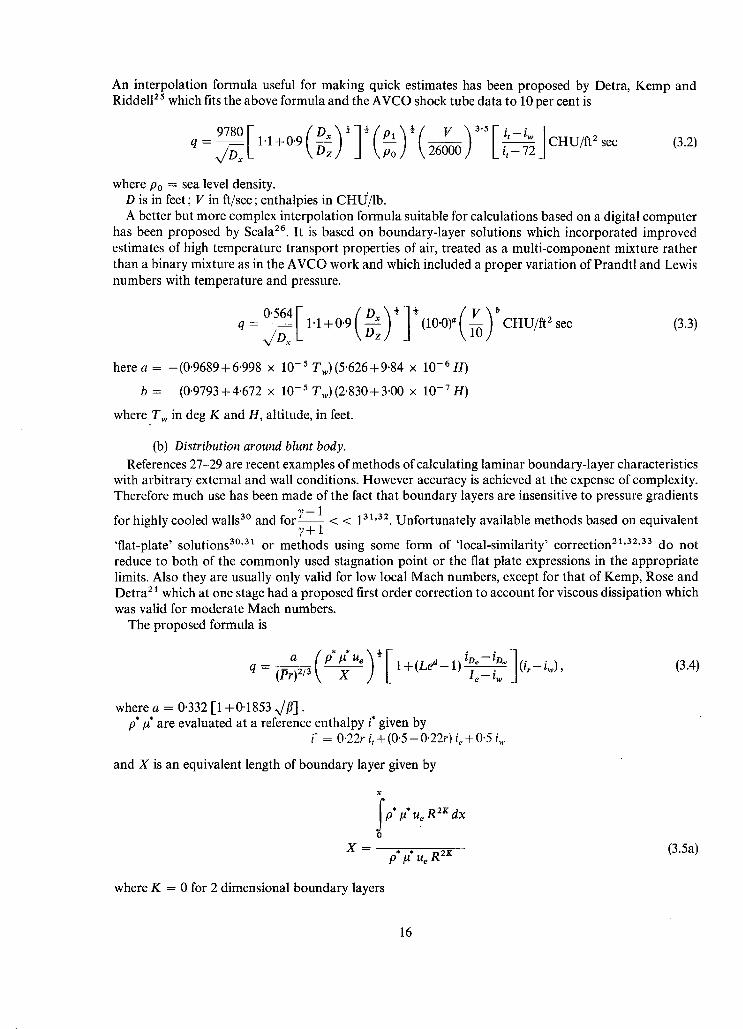
An interpolation formula useful for making quick estimates has been proposed by Detra, Kemp and RiddelF s which fits the above formula and the AVCO shock tube data to 10 per cent is

= 9780 F 1.1 +0.9 ( D ~ ½]~ | ~ l CHU/ft2 sec q ~ L ) ( ply½( V ~3"5Vi : n poJ \26000} Lt,-~zA

(3.2)

where Po = sea level density. D is in feet ; V in ft/sec; enthalpies in CHIJ/lb. A better but more complex interpolation formula suitable for calculations based on a digital computer

has been proposed by Scala 26. It is based on boundary-layer solutions which incorporated improved estimates of high temperature transport properties of air, treated as a multi-component mixture rather than a binary mixture as in the AVCO work and which included a proper variation of Prandtl and Lewis numbers with temperature and pressure.

0'564 + 0 . 9 ( D ~ ) ½ ] q~ b q=x/Dx [1'1 (10"0" ( V )

here a = -(0.9689+6.998 x 10 -5 Tw)(5"626+9"84 x 10-6H)

b = (0.9793+4.672 x 10 -5 Tw) (2.830+ 3.00 x 10-TH)

where T~ in deg K and H, altitude, in feet.

CHU/ft 2 sec (3.3)

(b) Distribution around blunt body. References 27-29 are recent examples of methods of calculating laminar boundary-layer characteristics

with arbitrary external and wall conditions. However accuracy is achieved at the expense of complexity. Therefore much use has been made of the fact that boundary layers are insensitive to pressure gradients

for highly cooled walls 3° and for 7v-~- ~ < < 131'32, Unfortunately available methods based on equivalent

'flat-plate' solutions a°'31 or methods using some form of 'local-similarity' correction 21'32'aa do not reduce to both of the commonly used stagnation point or the flat plate expressions in the appropriate limits. Also they are usually only valid for low local Mach numbers, except for that of Kemp, Rose and Detra 21 which at one stage had a proposed first order correction to account for viscous dissipation which was valid for moderate Mach numbers.

The proposed formula is

a ue 1 + (Le d- 1) (i,-iw), q = ~ X "e-tw A

(3.4)

where a = 0.332 [1 +0.1853 x/fl]" p* #* are evaluated at a reference enthalpy i* given by

i* = 0.22r it+(0"5-0"22r) i,,+0.5 i,,.

and X is an equivalent length of boundary layer given by

X =

f p" p* Ue R 2~ dx 0

p* #* U e R 2K (3.5a)

where K = 0 for 2 dimensional boundary layers

16

= 1 for axisymmetric boundary layers

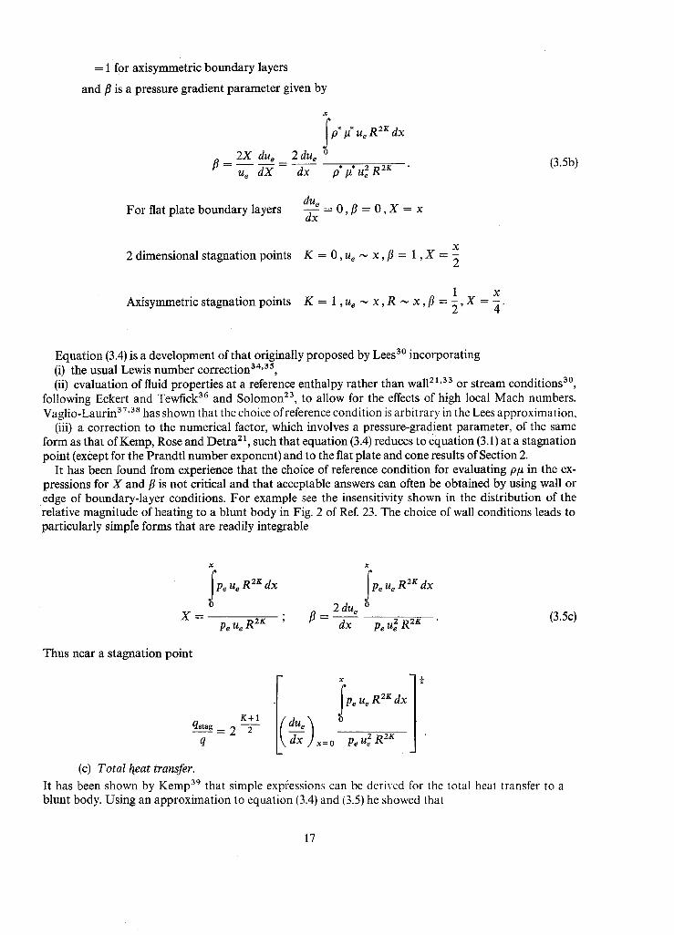
and fl is a pressure gradient parameter given by

x

f p* It* U e R 2K dx

/3 = 2 X due 2due o ue d X - dx p, #, u2 R2 K (3.5b)

For flat plate boundary layers due = 0,/3 = 0 , X = x dx

2 dimensional stagnation points X

K = O,u e'. , x , /3 = 1 , X = 2

1 X x Axisymmetric stagnation points K = 1, ue ~ x , R ,,~ x,/3 = 2 ' 4

Equation (3.4) is a development of that originally proposed by Lees 30 incorporating (i) the usual Lewis number correction 34'35, (ii) evaluation of fluid properties at a reference enthalpy rather than wall 21'33 or stream conditions 3°,

following Eckert and Tewfick 36 and Solomon z3, to allow for the effects of high local Mach numbers. Vaglio-Laurin 37'3s has shown that the choice of reference condition is arbitrary in the Lees approximation,

(iii) a correction to the numerical factor, which involves a pressure-gradient parameter, of the same form as that of Kemp, Rose and Detra 21, such that equation (3.4) reduces to equation (3.1) at a stagnation point (except for the Prandtl number exponent) and to the flat plate and cone results of Section 2.

It has been found from experience that the choice of reference condition for evaluating p# in the expressions for X and/3 is not critical and that acceptable answers can often be obtained by using wall or edge of boundary-layer conditions. For example see the insensitivity shown in the distribution of the relative magnitude of heating to a blunt body in Fig. 2 of Ref. 23. The choice of wall conditions leads to particularly simple forms that are readily integrable

x x

fpe eR x f eueR2K x o 2 du e o

X = " 13 = - - 2 R2K (3.5c) Pe Ue R2 r ' dx Pe Ue

Thus near a stagnation point

qstag _ _ 2 - -

q

(c) Total l~eat transfer.

K + I

2

Pe ue R 2K dx

due )

~-x x=0 7e~-~-J

It has been shown by Kemp 39 that simple exp?essions can be derived for the total heat transfer to a blunt body. Using an approximation to equation (3.4) and (3.5) he showed that

17

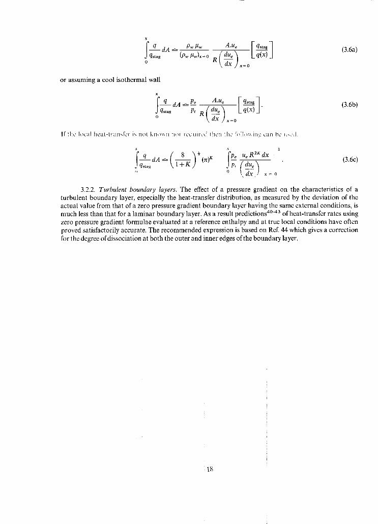
x

I q dA ~ Pw #w J qstag (Pw #w)x = o o

A'ue V qstag (due~ L q(x) ]

R \ dx /*=o

(3.6a)

or assuming a cool isothermal wall

x

f q dA.,,.P_2 qstag Pt

o

a . u e

R \ dx / .=o q - ~ ]

(3.6b)

lf lhc local hoat-tr'<lnsfcr is not kn~x~n mw required then lhc t~lh~x~ ii~ can bc u,cd

x

qstag (due~ 0 . \ c l x / ~ = o

(3.6c)

3.2.2. Turbulent boundary layers. The effect of a pressure gradient on the characteristics of a turbulent boundary layer, especially the heat-transfer distribution, as measured by the deviation of the actual value from that of a zero pressure gradient boundary layer having the same external conditions, is much less than that for a laminar boundary layer. As a result predictions 4°-43 of heat-transfer rates using zero pressure gradient formulae evaluated at a reference enthalpy and at true local conditions have often proved satisfactorily accurate. The recommended expression is based on Ref. 44 which gives a correction for the degree of dissociation at both the outer and inner edges of the boundary layer.

lg

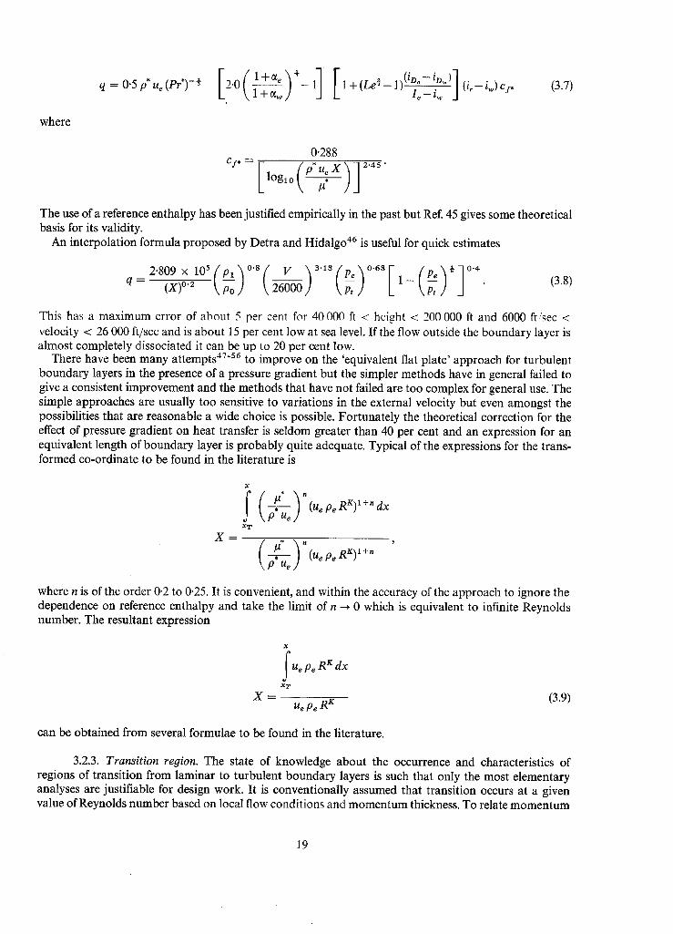
1•' I " ' q = 0 " 5 p ue(Pr*) -~ L-' \ 1 - - ~ / - l + ( L e ~ - I le-z~, / (3.7)

where

0.288 = C f, [ l °g l° ( p*ueXIA* )1 2-45"

The use of a reference enthalpy has been justified empirically in the past but Ref. 45 gives some theoretical basis for its validity.

An interpolation formula proposed by Detra and Hidalgo 46 is useful for quick estimates

q = 2"809 x 105(P-~oo)°'8( V 2 ~ 1 - ( ~ - t ) ~ l ° ' 4 . p e (3.8)

This has a maximum error of about 5 per cent for 40000 ft < height < 200000 ft and 6000 ft/sec < velocity < 26 000 ft/sec and is about 15 per cent low at sea level. If the flow outside the boundary layer is almost completely dissociated it can be up to 20 per cent low.

There have been many attempts ~7-s6 to improve on the 'equivalent flat plate' approach for turbulent boundary layers in the presence of a pressure gradient but the simpler methods have in general failed to give a consistent improvement and the methods that have not failed are too complex for general use. The simple approaches are usually too sensitive to variations in the external velocity but even amongst the possibilities that are reasonable a wide choice is possible. Fortunately the theoretical correction for the effect of pressure gradient on heat transfer is seldom greater than 40 per cent and an expression for an equivalent length of boundary layer is probably quite adequate. Typical of the expressions for the transformed co-ordinate to be found in the literature is

X =

p u~/ XT'

/~* )n - r - - (ue pe Rx) 1 +" P Ue

where n is of the order 0.2 to 0'25. It is convenient, and within the accuracy of the approach to ignore the dependence on reference enthalpy and take the limit of n ~ 0 which is equivalent to infinite Reynolds number. The resultant expression

x

r Ue Pe R r dx XT

X - Ue Pe Rr (3.9)

can be obtained from several formulae to be found in the literature.

3.2.3. Transition region. The state of knowledge about the occurrence and characteristics of regions of transition from laminar to turbulent boundary layers is such that only the most elementary analyses are justifiable for design work. It is conventionally assumed that transition occurs at a given value of Reynolds number based on local flow conditions and momentum thickness. To relate momentum

19

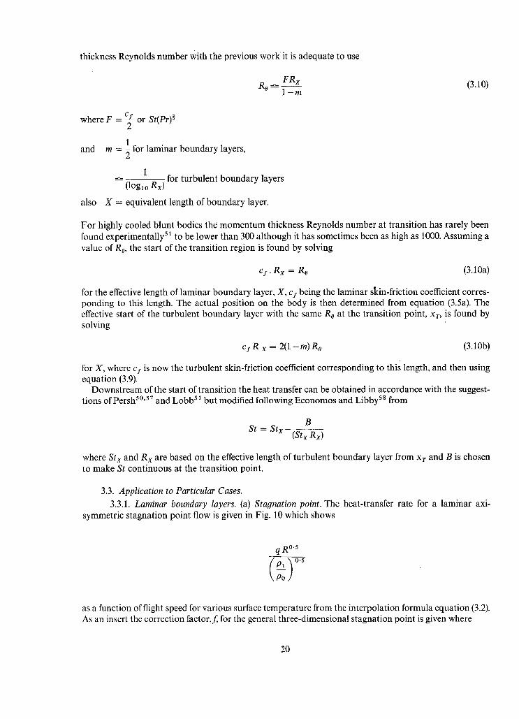
thickness Reynolds number With the previous work it is adequate to use

FRx e 0 ~ - -

1 - m (3.10)

where F = cl ~- or St(Pr) ~

1 and m = ~ for laminar boundary layers,

1 (log~o Rx) for turbulent boundary layers

also X = equivalent length of boundary layer.

For highly cooled blunt bodies the momentum thickness Reynolds number at transition has rarely been found experimentally 51 to be lower than 300 although it has sometimes been as high as 1000. Assuming a value of Ro, the start of the transition region is found by solving

cz. R x = Ro (3.10a)

for the effective length of laminar boundary layer, X, c s being the laminar s~in-friction coefficient corresponding to this length. The actual position on the body is then determined from equation (3.5a). The effective start of the turbulent boundary layer with the same Ro at the transition point, xr, is found by solving

c s R x = 2 ( 1 - m ) R o (3.10b)

for X, where c I is now the turbulent skin-friction coefficient corresponding to this length, and then using equation (3.9).

Downstream of the start of transition the heat transfer can be obtained in accordance with the suggest- tions ofPersh 5°'57 and Lobb 51 but modified following Economos and Libby 58 from

B St = S t x (StxRx)

where St x and R x are based on the effective length of turbulent boundary layer from Xr and B is chosen to make St continuous at the transition point.

3.3. Application to Particular Cases.

3.3.1. Laminar boundary layers. (a) Stagnation point. The heat-transfer rate for a laminar axisymmetric stagnation point flow is given in Fig. 10 which shows

q R 0"5

as a function of flight speed for various surface temperature from the interpolation formula equation (3.2). As an insert the correction factor,f, for the general three-dimensional stagnation point is given where

20

° '

For two-dimensional stagnation points the heating rates are 74 per cent of the axisymmetric values. If the body profile consists of a spherical or cylindrical segment cap followed by a discontinuity of slope

such that the tangent to the surface immediately downstream of the shoulder is less than 45 degrees to the freestream theft the above expressions will not apply unmodified because the stagnation point velocity gradient is then no longer given by the Newtonian expression. Limited experimental data for these cases are given in Refs. 20 and 59. The heating to a flat-faced body has been found experimentally to be 67 per cent of the heating to an equivalent hemisphere of the same radius as that of the flat face 6°.

(b) Distribution around blunt body. Equations (3.4) and (3.5) have been evaluated for two particular families of axisymmetric bodies that are

commonly met in i~r~ictice. Figs. 11 and 12 show the ratio of local heating to stagnation point heating q/q~ as a function of distance along the surface from the stagnation point for various Mach numbers for hemisphere-cylinders and hemispherically blunted cones respectively. A Newtonian type pressure distribution was assumed. Cone angles from 5 to 30 degrees were considered.

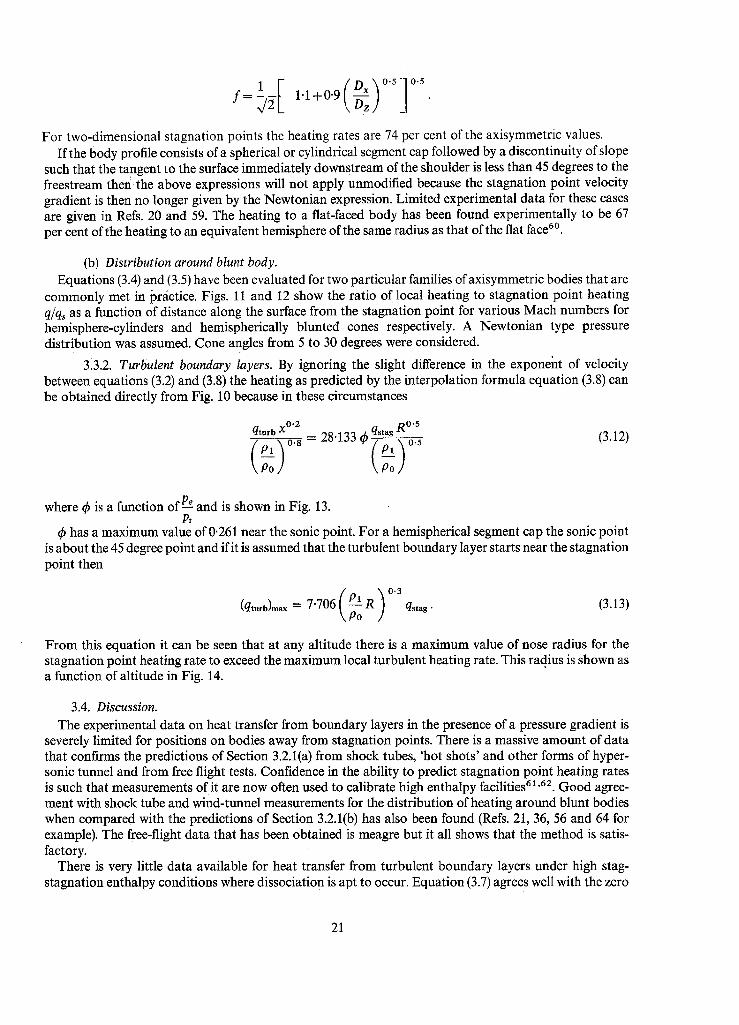
313.2. Turbulent boundary layers. By ignoring the slight difference in the exponent of velocity between equations (3.2) and (3.8) the heating as predicted by the interpolation formula equation (3.8) can be obtained directly from Fig. 10 because in these circumstances

qturb xO'2 ° ' 8

Po/

qstag RO' 5 (3.12)

where ~b is a function of ~ and is shown in Fig. 13. Pt

~b has a maximum value of 0.261 near the sonic point. For a hemispherical segment cap the sonic point is about the 45 degree point and if it is assumed that the turbulent boundary layer starts near the stagnation point then

(qturb)max = 7"706 R qstag" (3.13)

From this equation it can be seen that at any altitude there is a maximum value of nose radius for the stagnation point heating rate to exceed the maximum local turbulent heating rate. This radius is shown as a function of altitude in Fig. 14.

3.4. Discussion. The experimental data on heat transfer from boundary layers in the presence of a pressure gradient is

severely limited for positions on bodies away from stagnation points. There is a massive amount of data that confirms the predictions of Section 3.2.1(a) from shock tubes, 'hot shots' and other forms of hypersonic tunnel and from free flight tests. Confidence in the ability to predict stagnation point heating rates is such that measurements of it are now often used to calibrate high enthalpy facilities 61,62. Good agreement with shock tube and wind-tunnel measurements for the distribution of heating around blunt bodies when compared with the predictions of Section 3.2.1(b) has also been found (Refs. 21, 36, 56 and 64 for example). The free-flight data that has been obtained is meagre but it all shows that the method is satisfactory.

There is very little data available for heat transfer from turbulent boundary layers under high stag- stagnation enthalpy conditions where dissociation is apt to occur. Equation (3.7) agrees well with the zero

21

pressure gradient shock tube measurements of Ref. 53, Rely, 42 and 56 compare "equi~:tlcnt flat pl:tlc" formulae with the available wind-tunnel measurements quite favourably. No extensive comparison of the many possible forms of theory for turbulent boundary layer with a pressure gradient with the experi-

mental data has yet been made, but it has been done to some extent in Refs. 42 and 56. At present it may be considered that the status of methods for turbulent boundary layers in the presence

of pressure gradients is not satisfactory.

3.5. Further Comments.

3.5.1. Swept cylinders. The most recent studies of the laminar boundary layer on a swept cylinder are by Reshotko and Beckwith 64, Beckwith 22 and Cohen and Beckwith 65, and the application of this work is discussed in detail by Beckwith and Gallagher 66 and Wisniewski 13. These latter papers should be consulted for details of determining the local flow properties as well. At large free stream Mach numbers the effect of yaw is approximately given by (cos A) m.

At Reynolds numbers of the order of a few million and at yaw angles of 40 to 60 degrees Beckwith and Gallagher 6~' found that the boundarx laxer on a swept cylinder was completely turbulent even at the stagnation line. The level of heating rates and the nature of the chordwise distribution of heat transfer indic~tted that a flow mechanism different from the conventional transitional boundary layer may have existed at the intermediate yaw angles of 10 to 20 degrees. Ref. 66 presents a theory for the turbulent heating which is in reasonable agreement with its experimental data. Even with the turbulent boundary layer the peak heating rates occurred at the stagnation line.

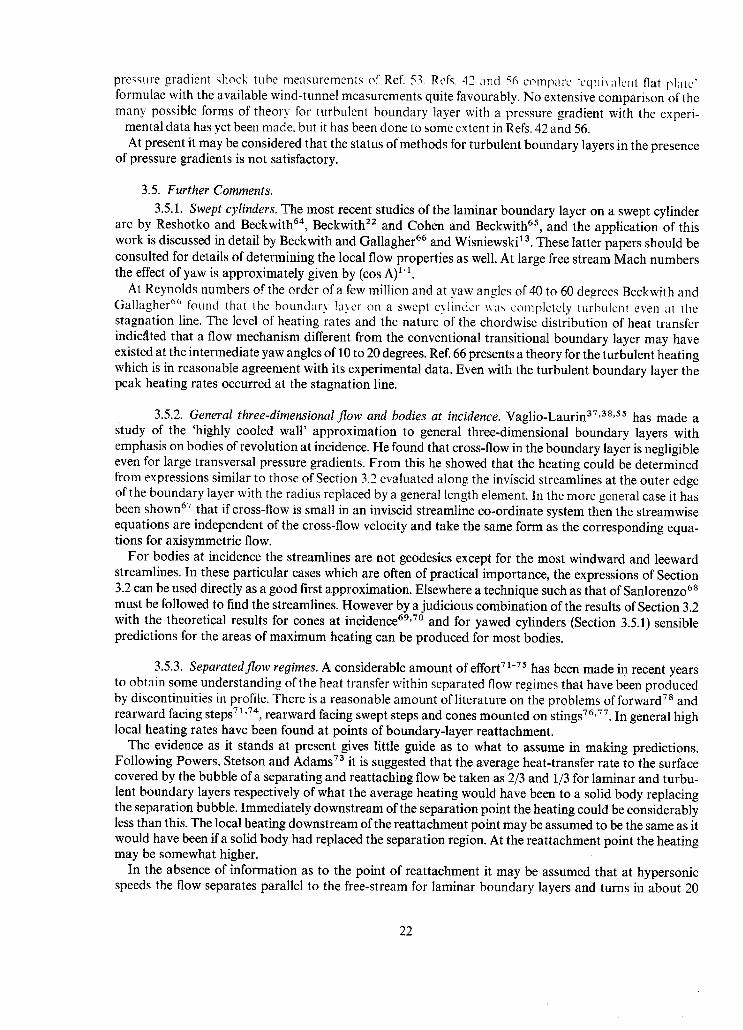
3.5.2. General three-dimensional flow and bodies at incidence. Vaglio-Laurin 37,38,5s has made a Study of the 'highly cooled wall' approximation to general three-dimensional boundary layers with emphasis on bodies of revolution at incidence. He found that cross-flow in the boundary layer is negligible even for large transversal pressure gradients. From this he showed that the heating could be determined from expressions similar to those of Section 3.2 evaluated along the inviscid streamlines at the outer edge of the boundary layer with the radius replaced by a general length element. In the more general case it has been shown 6~ that if cross-llow is small in an inviscid streamline co-ordinate system then the streamwise equations are independent of the cross-flow velocity and take the same form as the corresponding equations for axisymmetric flow.

For bodies at incidence the streamlines are not geodesics except for the most windward and leeward streamlines. In these particular cases which are often of practical importance, the expressions of Section 3.2 can be used directly as a good first approximation. Elsewhere a technique such as that of Sanlorenzo 68 must be followed to find the streamlines. However by a judicious combination of the results of Section 3.2 with the theoretical results for cones at incidence 69,7° and for yawed cylinders (Section 3.5.1) sensible predictions for the areas of maximum heating can be produced for most bodies.

3.5.3. Separated flow regimes. A considerable amount of effort 7 x-75 has been made in recent years to obtain some understanding of the heat transfer within separated flow regimes that have been produced by discontinuities in profile. There is a reasonable amount of literature on the problems of forward v 8 and rearward facing steps 71'74, rearward facing swept steps and cones mounted on stings 76'77. In general high local heating rates have been found at points of boundary-layer reattachment.

The evidence as it stands at present gives little guide as to what to assume in making predictions. Following Powers, Stetson and Adams 73 it is suggested that the average heat-transfer rate to the surface covered by the bubble of a separating and reattaching flow be taken as 2/3 and 1/3 for laminar and turbulent boundary layers respectively of what the average heating would have been to a solid body replacing the separation bubble. Immediately downstream of the separation point the heating could be considerably less than this. The local heating downstream of the reattachment point may be assumed to be the same as it would have been if a solid body had replaced the separation region. At the reattachment point the heating may be somewhat higher.

In the absence of information as to the point of reattachment it may be assumed that at hypersonic speeds the flow separates parallel to the free-stream for laminar boundary layers and turns in about 20

22

degrees for turbulent boundary layers. Stagnation points of the reversed flow on after bodies entirely immersed in the wake have been known 7~ to have heating rates of up to twice that predicted by the above proposal. Otherwise it is thought that the above rules of thumb will be conservative.

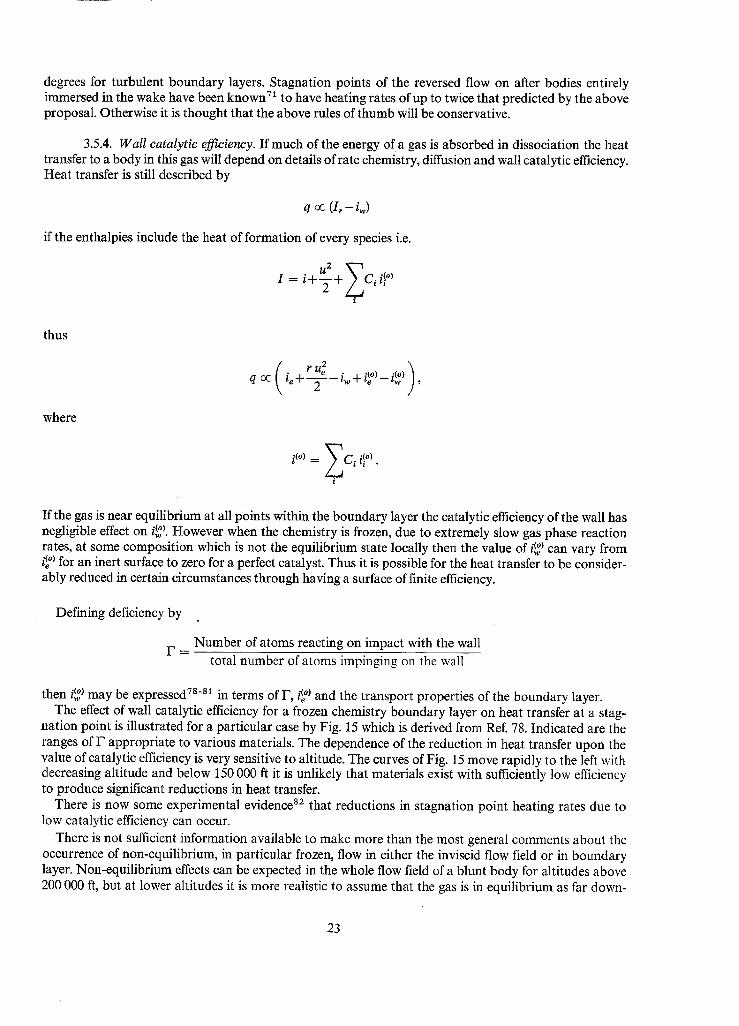
3.5.4. W a l l catalyt ic efficiency. If much of the energy of a gas is absorbed in dissociation the heat transfer to a body in this gas will depend on details of rate chemistry, diffusion and wall catalytic efficiency. Heat transfer is still described by

q o¢ f ir--iw)

if the enthalpies include the heat of formation of every species i.e.

u2 X I=i+T+ c, i! °~ i

thus

where

t r 2 i 4- r u e _ i .4. i(°) - - i(o) q oc - e - 2 v~,_.e ~w ] ,

i ~°~ = ~ C i i! °~ .

i

If the gas is near equilibrium at all points within the boundary layer the catalytic efficiency of the wall has negligible effect on i (°). However when the chemistry is frozen, due to extremely slow gas phase reaction rates, at some composition which is not the equilibrium state locally then the value of i~ ) can vary from i~ ) for an inert surface to zero for a perfect catalyst. Thus it is possible for the heat transfer to be considerably reduced in certain circumstances through having a surface of finite efficiency.

Defining deficiency by

F = Number of atoms reacting on impact with the wall

total number of atoms impinging on the wall

then i~ ) may be expressed 7s'sl in terms of F, i(fl ) and the transport properties of the boundary layer. The effect of wall catalytic efficiency for a frozen chemistry boundary layer on heat transfer at a stag-

nation point is illustrated for a particular case by Fig. 15 which is derived from Ref. 78. Indicated are the ranges of F appropriate to various materials. The dependence of the reduction in heat transfer upon the value of catalytic efficiency is very sensitive to altitude. The curves of Fig. 15 move rapidly to the left with decreasing altitude and below 150 000 ft it is unlikely that materials exist with sufficiently low efficiency to produce significant reductions in heat transfer.

There is now some experimental evidence 82 that reductions in stagnation point heating rates due to low catalytic efficiency can occur.

There is not sufficient information available to make more than the most general comments about the occurrence of non-equilibrium, in particular frozen, flow in either the inviscid flow field or in boundary layer. Non-equilibrium effects can be expected in the whole flow field of a blunt body for altitudes above 200 000 ft, but at lower altitudes it is more realistic to assume that the gas is in equilibrium as far down-

23

stream as the sonic line after which it may be assumed to be frozen at the composition at the sonic line. However downstream of the sonic point on the body the temperatures in the boundary layer can be higher than those in the external flow and as a consequence the composition near the surface will be nearer local equilibrium than the composition of the external flow will be.

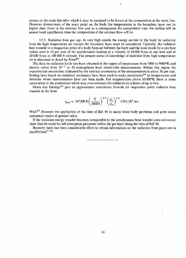
3.5.5. Radiation from gas cap. At very high speeds the energy carried to the body by radiation from the high temperature air outside the boundary layer must be considered. Typically, the radiative heat transfer to a stagnation point of a body from air between the body and the nose shock for a one foot radius nose is 10 per cent of the aerodynamic heating at a velocity of 10 000 ft/sec at sea level and at 20 000 ft/sec at 100 000 ft altitude. The present status of knowledge of radiation from high temperature air is discussed in detail by Kive183.

The data on radiation levels has been obtained in the region of temperature from 5000 to 9000°K and density ratios from 10 -2 to 10 atmospheres from shock-tube measurements. Within this region the experimental uncertainty indicated by the internal consistency of the measurements is about 30 per cent. Scaling laws based on statistical mechanics have been used to make predictions 84 at temperatures and densities where measurements have not been made. For temperatures above 10 000°K there is some uncertainty in the predictions which may over-estimate the radiation by a factor of up to two.

Detra and Hidalgo 46 give an approximate correlation formula for stagnation point radiative heat transfer in the form

/z V ~ 8"5 ( p l ) 1"6 qr.a = 187200 R ~ ~ ) Po CHU/ft a sec.

Wick a5 discusses the application of the data of Ref. 84 to many blunt body problems and gives many numerical results of general value.

If the radiation energy transfer becomes comparable to the aerodynamic heat transfer some allowance must then be made for self absorption processes within the gas layer along the lines of Ref. 86.

Recently there has been considerable effort to obtain information on the radiation from gases not in equilibrium s7-9°.

24

A

a,b,d

C

Cf

Cp

D

f

h

H

i

i*

i(o)

I

J

k

Le

M

m~ Tl

Nu, Nu'

P

Pr

Q~

q

LIST OF SYMBOLS

Surface area (ft 2) up to the point x, or surface area of blunt body

Used as constants or exponents

Concentration of a species in a gas

Local skin-friction coefficient = %1½Pel ue2 A

if Mean skin-friction coefficient = ~ c: dA

0

_f ~C'H'U" ) Specific heat of air at constant pressure ~ ~ 0.24 × 32.2

Diameter

A function of Section 3.3.1

Heat transfer factor--see (1 1) oquatioo ( ) Altitude T

c dT: enthalpy of the air at temperature T 0

'Intermediate' enthalpy--see equation (1.3)

Energy of formation of a species in a gas

Total enthalpy

ftlb Mechanical equivalent of heat \ C_H_U. ,]

Thermal conductivity of air ( °KC'H'U'ft sec ] )

Lewis number

Mach number

Exponents in equations (3.10) and (3.14)

Nusselt numbers, based on enthalpy difference and temperature difference respectively-- see equations (1.7) and (1.Ta)

Pressure

Prandtl number ( = ~ ) .

Solar radiation constant

Rate of convective heat transfer per unit area \ ft 2 sec

25

qr

R

r

LIST OF SYMBOLS---continued

Rate of heat loss by radiation per unit area ft 2 sec

Local radius of body (Section 3)

Enthalpy recovery factor

R e

R~

Ro

St, St'

T

u

V

x

:(

~s

O~

3

Y

F

8G

9

#

P

Subscripts

b

eq

Reynolds number

Local Reynolds number based on transformed distance X (Section 3)

Local Reynolds number based on momentum thickness

Local Stanton numbers (non-dimensional heat transfer coefficients) based on enthalpy difference and temperature difference respectively--see equations (1-6) and (1.6a)

Temperature (°K)

Local air speed (ft/sec)

Free stream velocity

Distance along surface (ft) along a geodesic or along inviscid streamline external to boundary layer

Transformed distance of equations (3.5a) and (3.9)

Absorption factor for solar radiation

Proportion of atoms to total number of particles present

Pressure-gradient parameter of equation (3.5b)

Ratio of specific heats of air

Catalytic efficiency of a surface

Surface emissivity factor

Gas emissivity factor

Angle between normal to surface and incident rays of sun

slug Viscosity of air \ ~ }

_ / slug '~ Density ot air ~ ~ )

A function given in equation (3.12) and Fig. 13

Surface shear stress ( f~2 )

Empirical values in formula for p~t, Section 3.2.1(a)

Equilibrium conditions

26

i

w

r

X

e

1

s

t

K = 0

= 1

Superscript

LIST OF SYMBOLS--continued

Incompressible flow (Sections 1 and 2), or individual species of a gas (Section 3)

Conditions at the wall

Recovery conditions, i.e. conditions at the wall for zero heat transfer

Conditions at distance x along surface

Local conditions in external flow at edge of boundary layer

Free stream conditions (ahead of bow shock)

Stagnation conditions (Sections 1 and 2), or conditions at sonic point of body (Section 3)

Conditions at sonic point of body (Section 3) total conditions (Section 3)

For 2-dim. boundary layers

For axisymmetric boundary layers

Corresponding to the 'intermediate' enthalpy i*

27

REFERENCES

No. Author(s)

1 E.R.G. Eckert ..

2 R.J. Monaghan . . . .

3 R.A. Minzner and W. S. Ripley

4 Fishenden and Saunders ..

5 Boelter, Brennan, Bromberg .. and Gier

7 P.A. Libby and R. J. Cresci

8 M.O. Creager . . . .

9 B. Kivel and K. Bailey

10 T. Tendeland . . . .

11 R.K. Lobb, E. M. Winkler and J. Persh


Title, etc.

Survey on heat transfer at high speeds. WADC Technical Report 54-70, April 1954.

Formulae and approximations for aerodynamic heating rates in high speed flight.

A.R.C.C.P. 360, October 1955.

The ARDC Model Atmosphere, 1956. Air Force Surveys in Geophysics No. 86, AFCRC, T.N. 56-204. Astia Document No. 110233, December 1956. Geophysics Research Directorate, Air Force, Cambridge Research

Center, Bedford, Mass. See also 1959 edition.

The calculation o f heat transmission. HMSO, 1932, pp. 1-57.

An investigation of aircraft heaters. XXXII. The mean effective emissivity as a function of temperature

for several metals. NACA ARR, University of California.

Heating, ventilating and air conditioning guide. American Society of Heating and Ventilating Engineers.

Evaluation of several hypersonic turbulent heat transfer analyses by comparison with experimental data.

WADC T.N. 57-72, Astia Document No. A.D. 118093.

Effects of leading-edge blunting on the local heat transfer and pressure distributions over flat plates in supersonic flow.

NACA T.N. 4142, December 1957.

Tables of radiation from high temperature air. Research Report 21, December 1957. AVCO Research Laboratory, Everett, Mass.

Effects of Mach number and wall-temperature ratio on turbulent heat transfer at Mach numbers from 3 to 5.

NACA T.N. 4236, April 1958.

Experimental investigation of turbulent boundary layers in hypersonic flow.

Journ. Aero. Sciences, Vol. 22, No. 1, pp. 1-9. January 1955.


WADC T.N. 57-72, Astia Document No. AD.118093.

28

No. Author(s)

13 M.O. Creager . . . .

14 Hartnett, Eckert, Birkebak and Sampson

15 Eckert, Hartnett and Birkebak

16 D.B. Spalding . . . . ..

17 J. A. Fay, F. R. Riddell and .. N. H. Kemp

18 J.A. Fay and F. R. Riddell ..

19 E. Reshotko . . . . . .

20 R.J. Wisniewski . . . .

21 N.H. Kemp, P. H. Rose and. . R. W. Detra

22 I.E. Beckwith . . . . . .

23 J.M. Solomon . . . . . .

24 N.B. Cohen . . . . . .

2_5 R.W. Detra, N. H. Kemp and

REFERENCES--continued

Title, etc.

Effects of leading-edge blunting on the local heat transfer and pressure distributions over flat plates in supersonic flow.

NACA T.N. 4142, December 1957.

Simplified procedures for the calculation of heat translbr to surfaces with non-uniform temperatures.

WADC Technical Report 56-373, July 1956. (Astia Document No. 110450).

The calculation of the wall temperature along surfaces which are exposed to a fluid stream when the local heat flow through the surfaces is prescribed.

WADC Technical Report 57-315 (Astia Document No. 118333) May 1957.

Heat transfer from surfaces of non-uniform temperature. Journ. Fluid Mech., 4, p. 22, May 1958.

Stagnation point heat transfer in dissociated air flow. Jet Propulsion Vol. 27, No. 6, p. 672. June 1957.

Theory of stagnation point heat transfer in dissociated air. J. Aero. Sc., Vol. 25, No. 2, p. 73, February 1958.

Heat transfer to a general three dimensional stagnation point. Jet Propulsion, Vol. 28, No. 1, p. 58, January 1958.

Methods of predicting laminar heat rates on hypersonic vehicles. NASA TN.D-201, December 1959.

Laminar heat transfer around blunt bodies in dissociated air. J. Aero/Space Sc. Vol. 26, No. 7, p. 421 July 1959. Also AVCO Res. Lab. Res. Rept. 15, May 1958.

Similar solutions for the compressible boundary layer on a yawed cylinder with transpiration cooling.

NACA TN.4345, September 1958.

Approximate calculation of the equilibrium 'laminar boundary layer On blunt bodies at hypersonic speeds.

ARS Journal, Vol. 32, No. 3, p. 422, March 1962.

Correlation formulae and tables of density and some transport properties of equilibrium dissociating air for use in solutions of the boundary layer equations.

NASA TN.D-194, February 1960.

Addendum to 'Heat transfer to satellite vehicles re-entering the

29

No. Author(s)

F. R. Riddell

26 S.M. Scala . . . . . .

27 N. Curle . . . . . .

28 G.M. Lilley ..

29 R.J. Monaghan . . . .

30 L. Lees . . . . . . . .

31 F.K. Moore and H. K. Cheng..

32 F.K. Moore . . . . . .

33 R.F. Probstein

34 L. Lees . . . .

35 R. Bromberg and R. P. Lipkis

36 E.R.G. Eckert and .. O. E. Trewfik

37 R. Vaglio-Laurin . . . .


Title, etc.

atmosphere'. Jet Propulsion, Vol. 27, No. 12, p. 1256, December 1957.

Hypersonic ablation. Preprint at 10th International Astronautical Congress. London,

September 1959.

The steady compressible laminar boundary layer with arbitrary pressure gradient and uniform wall temperature.

Proc. Roy. Soc. (A) Vol. 249, p. 206, 1958.

A simplified theory of skin friction and heat transfer for a compressible laminar boundary layer.

College of Aeronautics Note 93, January 1959. A.R.C. 21729.

Effects of heat transfer on laminar boundary layer development under pressure gradients in compressible flow.

A.R.C.R. & M. 3218, May 1960.

Laminar heat transfer over blunt-nosed bodies at hypersonic flight speeds.

Jet Propulsion, Vol. 26, No. 4, p. 259, April 1956.

The hypersonic aerodynamics of slender and lifting configurations. IAS Paper No. 59-125, June 1959.

On local flat-plate similarity in the hypersonic boundary layer. J. Aerospace Sciences, Vol. 28, No. 10, p. 753, October 1961.

Methods of calculating the equilibrium laminar heat transfer rate at hypersonic flight speeds.

Jet Propulsion, Vol. 26, No. 6, p. 497, June 1956.

Convective heat transfer with mass addition and chemical reactions.

3rd AGARD Colloquium on Combustion, p. 451, Palermo, March 1958.

Heat transfer in boundary layers with chemical reactions due to mass additions.

Jet Propulsion, Vol. 28, No. 10, p. 668, October 1958.

Use of reference enthalpy in specifying the laminar heat transfer distribution around blunt bodies in dissociated air.

J. Aero/Space Sc., Vol. 27, No. 6, p. 464, June 1960.

Laminar heat transfer on three dimensional blunt nosed bodies in

30

No. Author~)

38 R. Vaglio-Laurin ..

39 N.H. Kemp . . . .


41 A. Ferri . . . . . .

42 N.B. Cohen . . . .

43 H. Hidalgo . . . .

44 W.H. Dorrance ..

45 O.R. Burggraf . . . .

• °


Title, etc.

hypersonic flow. ARS Journal, Vol. 29, No. 2, p. 123, February 1959.

Heat transfer on blunt nosed bodies in general three dimensional hypersonic flow.

Heat Transfer and Fluid Mechanics Institute, p. 95, 1959.

Note on the surface integral of laminar heat flux to symmetric bodies at zero incidence.

ARS Journal, Vol. 32, No. 4, p. 639, April 1962.


Polytechnic Institute of Brooklyn WADC TN-57-72, July 1957.

A review of some recent developments in hypersonic flow. 1st International Congress in the Aeronautical Sciences, Madrid,

September 1958. Advances in Aeronautical Sciences, Vol. II. Editor T. von Karman,

Pergamon Press, London, 1959.

A method of computing turbulent heat transfer in'the presence of a streamwise pressure gradient for bodies in high speed flow.

NASA Memo 1-2-59L, March 1959.

Closing reply to comment on 'Generalized heat transfer formulae and graphs for nose-cone re-entry into the atmosphere' by Sibulkin.

ARS Journal, Vol. 32, No. 4, p. 647, April 1962.

Dissociation effects upon compressible turbulent boundary layer skin friction and heat transfer.

ARS Journal, Vol. 31, No. 1, p. 61, January 1961.

The compressibility transformation and the turbulent boundary layer equations.

J. Aero/Space Sc., Vol. 29, No. 4, p. 434, April 1962.

46 R.W. Detra and H. Hidalgo. .

47 F.E.C. Culick and J. A. F. Hill

48 A. Mager . . . . . .

Generalized heat transfer formulae and graphs for nose cone re-entry into the atmosphere.


A turbulent analog of the Stewartson-Illingworth transformation. J. ofAero Sc., Vol. 25, No. 4, p. 259, April 1958.

Transformation of the compressible turbulent boundary layer. J. ofAero Sc., Vol. 25, No. 5, p. 305, May 1958.

31

No. Author(s)

49 E. Reshotko and M. Tucker ..

50 J. Persh . .

51 R.K. Lobb

52 M.R. Denison

53 P. H. Rose, R. F. Probstein and C. M. C. Adams

54 R.L. Phillips . . . . . .


Title, etc.

Approximate calculation of the compressible turbulent boundary layer with heat transfer and arbitrary pressure gradient.

NACA TN.4154, December 1957.

A theoretical investigation of turbulent boundary layer flow with heat transfer at supersonic and hypersonic speeds.

Navord Rpt. 3854, also Proceedings of 4th Mid West Conf. on Fluid Mechanics, p. 43,

September 1955.

Aerodynamic heating of hypersonic bodies. Supplementary paper at Tri-Partite Conf. Session A.l(c), London

1957.

Turbulent boundary layer on blunt bodies of revolution at hypersonic speeds.

Lockheed Aircraft Corp. Missile Systems Division, April 1956.

Turbulent heat transfer through a highly cooled, partially dissociated boundary layer.

Jet Propulsion, Vol. 28, No. 1, p. 56, January 1958. Journal,ofAero/Spaee Sc., Vol. 25, No. 12, p. 751, December 1958.

A summary of several techniques used in the analysis of high- enthalpy level, high cooling ratio turbulent boundary layers on blunt bodies of revolution.

Ramo-Wooldridge Report GM-TM-194, September 1957.

55 R. Vaglio-Laurin . . . .

56 R. J. Cresci, D. A. MacKenzie.. and P. A. Libby

57 J. Persh . . . . . . . .

58 C. Economos and P. A. Libby

59 J.C. Boison and H. A. Curtiss

Turbulent heat transfer on blunt-nosed bodies in two-dimensional and general three-dimensional hypersonic flow.

J. ofAero/Space Sc., Vol. 27, No. 1, p. 27, January 1960 also WADC TN 58-301, September 1958.

An investigation of laminar, transitional and turbulent heat transfer on blunt nosed bodies in hypersonic flow.

J. ofAero/Spaee Sc., Vol. 27, No. 6, p. 401, June 1960.

A procedure for calculating the boundary layer development in the region of transition from laminar to turbulent flow.

USNOL Navord Rpt. 4438, March 1957.

A note on transitional heat transfer under hypersonic conditions. J. Aero/Space Se., Vol. 29, No. 1, p. 101, January 1962.

An experimental investigation of blunt body stagnation point velocity gradient.

ARS Journal, Vol. 29, No. 2, p. 130, February 1959.

32

No. Author(s)

60 W.E. Stoney . . . .

61 T.R. Brogan . . . .

62 R.R. John and W. L. Bade

63 J . C . B o i s o n . . . .

64 E. Reshotko and I. E. Beckwith

65 N.B. Cohen and I. E. Beckwith

66 I.E. Beckwith and J. E. Gallagher

67 J.C. Cooke and M. G. Hall

68 E.A. Sanlorenzo ..

69 E. Reshotko . . . .

70 W.H. Braun . . . .

71 J. Rabinowicz . . . .


Title, etc.

Aerodynamic heating of blunt nose shapes at Mach numbers up to 14.

NACA RM L58E05a (TIL 6125), August 1958.

The electric-arc wind tunnel--a tool for atmospheric re-entry research.

ARS Journal, Vol. 29, No. 9, p. 648, September 1959.

Recent advances in electric-arc plasma generation technology. ARS Journal, Vol. 31, No. 1, p. 4, January 1961.

Experimental investigation of the hemisphere cylinder at hyper- velocities in air.

AEDC-TR-58-20, November 1958.

Compressible laminar boundary layer over a yawed infinite cylinder with heat transfer and arbitrary Prandtl number.

NACA Rpt. 1379 (formerly TN.3986), 1957.

Boundary layer similar solutions for equilibrium dissociated air and application to the calculation of laminar heat transfer distribution on blunt bodies in high speed flow.

International Development in heat transfer. Part II, Section B, p. 406.

1961 International heat transfer conference. Colorado August 1961 and Westminster, January 1962.

Local heat transfer and recovery temperature on a yawed cylinder at a Mach number of 4.15 and high Reynolds numbers.

NASA TR.R.104, 1961.

Boundary layers in three dimensions. R.A.E. Report Aero 2635, A.R.C. 21 905. 1960.

Method for calculating surface streamlines and laminar heat transfer to blunted cones at angle of attack.

3. Aero/Space Sc., Vol. 28, No. 11, p. 904, November 1961.

Laminar boundary layer with heat transfer on a cone at angle of attack in a supersonic stream.

NACA TN 4152, December 1957.

Turbulent boundary layer on a yawed cone in a supersonic stream. NACA TN.4208, January 1958.

Measurement of turbulent heat transfer rates on the aft portion and blunt base of a hemisphere cylinder in a shock tube.

Jet Propulsion, Vol. 28, No. 9, p. 615, September 1958.

33

No. Author(s)

72 M.H. Bloom and A. Pallone..

73 H.K. Larson . . . . . .

74 A. Nayswith . . . . . .

75 G.E. Gadd and J. L. Attridge

76 A. Naysmith . . . .

77 J. Picken . . . .

78 R. Goulard . . . .

79 D.E. Rosser . . . .

80 P.M. Chung and A. D. Anderson

81 D.E. Rosner . . . . . .

82 J.B. Busing . . . . . .


Title, etc.

Shroud tests of pressure and heat transfer over short afterbodies with separated wakes.

J. Aero/Space Sc., Vol. 26, No. 10, p. 626, October 1959.

Heat transfer in separated flows. J. Aero/Space Sc., Vol. 26, No. 11, p. 731, November 1959.

Heat transfer and boundary layer measurements in a region of supersonic flow separation and reattachment.

R.A.E. Tech Note Aero 2558, May 1958. A.R.C. 20 601.

Heat transfer and skin friction measurements at a Mach number of 2.44 for a turbulent boundary layer on a flat surface and in regions of separated flow.

A.R.C.R. & M. 3148, October 1958.

Measurements of heat transfer in bubbles of separated flow in supersonic airstreams.

International Development in heat transfer, Part II, Section B, p. 378, August 1961.

Free-flight measurements of pressure and heat transfer in regions of separated and reattached flow at Mach numbers up to 4.

R.A.E. Report Aero 2643, September 1960. A.R.C. 22 618.

On catalytic recombination rates in hypersonic stagnation heat transfer.

Jet Propulsion, Vol. 28, No. 11, p. 737, November 1958.

Similitude treatment of hypersonic stagnation heat transfer ARS Journal, Vol. 29, No. 3, p. 215, March 1959.

Surface recombination in the frozen compressible flow of a dissociating diatomic gas past a catalytic flat plate.


Surface temperatures of high speed radiation cooled bodies in dissociating atmospheres.

ARS Journal, Vol. 31, No. 7, p. 1013, July 1961.

The effect of catalytic surfaces on stagnation point heat transfer in partially dissociated flows, preprint AGARD specialists meeting.

The high temperature aspects of hypersonic flow, Brussels, April 1962. Pergamon Press, 1963.

34

No. Author(s)

83 B. Kivel . . . .

84 B. Kivel and K. Bailey ..

85 B.H. Wick . . . . . .

86 H. Kennett and S. L. Strack ..

87 J.C. Carom, B. Kivel,.. .. R. L. Taylor and J. D. Teare

88 J D. Tcurc. % (ieorgiev :lnd .. R. Allen

89 C.E. Treanor . . . . . .

90 P.H. Rose and J. D. Teare ..


Title, etc.

Radiation from hot air and its effect on stagnation point heating. J. Aero/Space Sc., Vol. 28, No. 2, p. 96, February 1961, and AVCO Res. Rpt. 79, October 1959.

Radiation from high-temperature air. AVCO Res. Rept. 21, January 1958.

Radiative heating of vehicles entering the Earths atmosphere. Preprint at AGARD specialists meeting The high temperature

aspects of hypersonic flow, Brussels, April 1962. Pergamon Press 1963.

Stagnation point radiative transfer. ARS Journal, Vol. 31, No. 3, p. 370, March 1961.

Absolute intensity of non-equilibrium radiation in air and stagnation heating at high altitudes.

AVCO Res. Rpt. 93, December 1959 and AVCO Res. Note 175, December 1959.

Radiation from non-equilibrium shock front. ARS preprint 1979-61. International Hypersonic Conference M I T, August 1961.

Radiation at Hypersonic Speeds. ARS preprint 1978-61. International Hypersonic Conference M I T, August 1961.

On chemical effects and radiation in hypersonic aerodynamics. Preprint at AGARD specialists' meeting. The high temperature aspects of hypersonic flow, Brussels, April

1962. Pergamon Press 1963.

35

L*J C~

106xl Z-4

Z ' 0

1"6

St i x i0]

I - 2

0-8

0-4

0 I() 5 x

107xl

" ° ==6 6,~ I

Re x (Turbulent) 108 x I

r~ x ( u ; ~ i . ~ r ) . . . . ~16txl

109x I

108x l

FIG. l. S tanton numbers for a flat plate in incompressible flow.

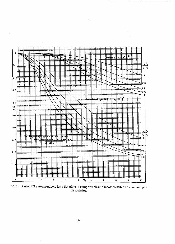
FIG. 2. Ratio of Stanton numbers for a flat plate in compressible and incompressible flow assuming no dissociation.

37

I (~3 ,

7

- 4 I 0 ;

hx

i f 2, 9

8

7

6

S

h x

slugs ~ ft..sec/

2

9

8

7

6

S

4

S

e

7

5

S

4

s, 9

S

7

6

S

4

3

I 2

I J

8

7

6

S

4

3

2

FIG. 4. Local heat transfer factor on a flat plate--turbulent boundary layer.

39

30

N

( I r --

C.I- slL

ZO.

5~

I O,

5~

I'0 2"0 3-0 4"0 5.0 6"0 7-0 8-0 U $ |¢C

I000

9-0

FIG. 5. Enthalpy at the wall under conditions of zero heat transfer.

40,

10"0

~ 5

24.'

23'

21

20-_

Je: 17.

Ig"

is:

14"::

12-"

II

lo-

s2

~oA-' gl

F. 3.

2.

!

~"r/L e

ZO-

19

15

17-

IG-

IS-

1 4

13'

IO.

9 .

B"

7-

6

5"

4"

3"

2"

"27

26

'25

"24

23

| 9

-17

"16

15

14

13

: u

'10

9

- 8

:7 . 6

. 5

"4

is .!

, FIG. 6. Nomogram f o r d e t e r m i n a t i o n o f i n t e r m e d i a t e enthalpy, i*/i e = I + 0 '5 (i,,./i e - 1)+ 0 .22 ( i r / i e - 1).

41

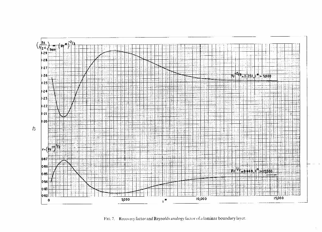
.[~ b.~

FIG. 7. Recovery factor and Reynolds analogy factor of a laminar boundary laycr.

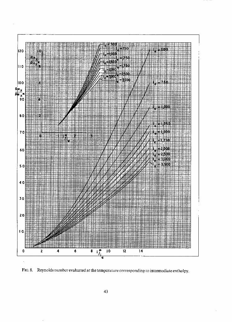
FIG. 8. Reynolds number evaluated at the temperature corresponding to intermediate enthalpy.

43

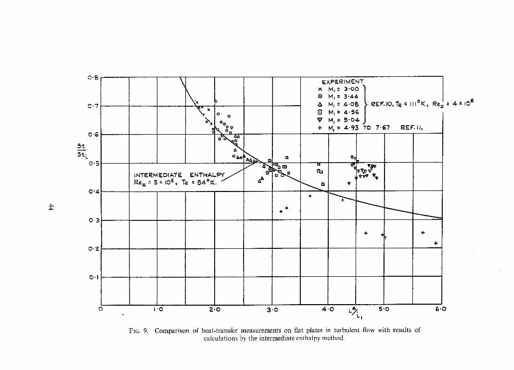
4~

o.B

C.7

o.~

5 t

5~ L 0.5

0"4

0"3

0"~

O'1

O

EAPERIMENT x Mt = 3 .00

~ . = (9 MI = 3"4.4. & Mj = 4 "08 ; t~EF.IO, Te = I I l °K~ Re.

e r;I Mr= 4 "56 ® ®® ~ M I = 5 " 0 ~

e e + M t = 4.'95 TO 7"67 REF'.II~

AA . ~ ,vW % - . . . < = ,

INTERMEDIATE ENTHA, L P Y J Re..c= 5x lOS~ Te = 8 4 ° K . /

÷

FIG. 9.

I 0 2.0 3-0 ,4"0 ~'~'E. ~ 5"0 6'0

Comparison of heat-transfer measurements on flat plates in turbulent flow with results of calculations by the intermediate enthalpy method.

.- 4 . X l O 6

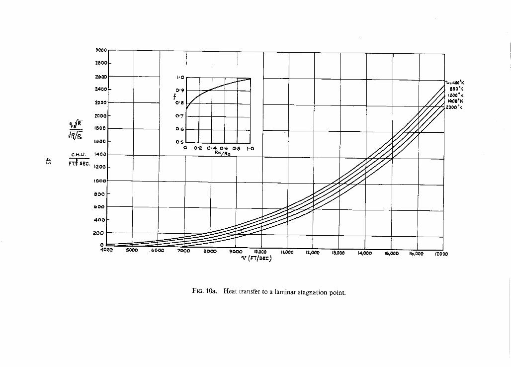
Je,/~

C.H.U.

3000 •

2800 - 1 Z(oO0

Z400

2zOO

ZOO0

1800

I.~o00

14o0

120o

IOOO

80O

~00

ZOO

0

/ f ~

0 0"2. 0 "4 0"~ 0 '8 I ' 0 R~(/Rz

S 4000 $000 6000

!

7 J / ~ " ,.. YJ7

J

!

r

~ooo eooo 9 0 0 0 , . o ,,.ooo ~z.ooo ,~.ooo i

14,00o tS, O00 I (o ,000 17,000

r.:4OO'K 8oo°K

t200°K |600eK

ZO00"~

FIG. lOa. Heat transfer to a laminar stagnation point.

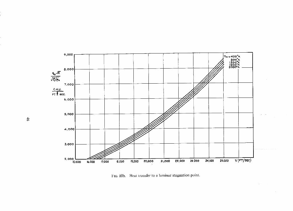
9 ,000

8 , 0 0 C %.gff

~,/eo 7 , 0 0 0

C.H.U. 3

FT i SEC,

5 , 0 0 0

5, 0 0 0

~ . ,000

3 , 0 0 0

2, 000 15,OO0 Ib,O00 rT, ooo tB,O0O 19,000 zo,ooo z l ,o00 Z2,O0O 2..a, O00 24,000

Y 'Tw = 4 0 0 o~

800°Y, 1200':'K I,~O0°K ZOO0 ° K

z~,ooo v (r'r/sF.c)

FIO. lOb. Heat transfer to a laminar stagnation point.

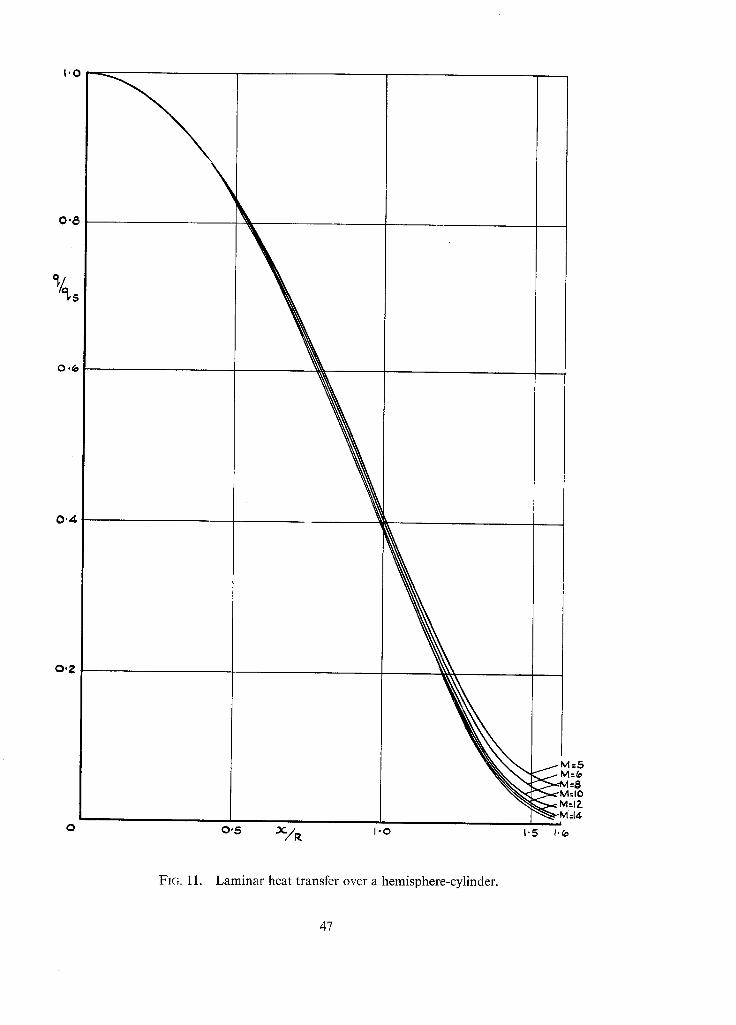
I'O

0.~

0.~

0'4

0'2

0 0-5 ~c/~ i.o

~M:IO 1.5 t.~

Fie,. 11. Laminar heat transfer over a hemisphere-cylinder.

47

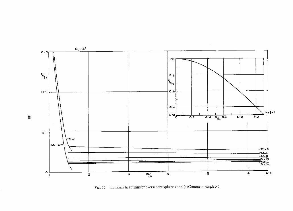
c~

Qr/~S

0 . 2

0"1

0

GC = 5 °

-M=5

L_

X

S

'4

"5 0 0 . 2

t I 0 . 4 X/R " 0.(o

I O.S

Z 3 =~/R 4 5

\ l \ M = 5 - I

I ' 0

-"M= 5

- M = 8 -IM = IO

\M=I? . M= [4

1 (o ~ ' 5

FIG. 12. Laminar heat transfer over a hemisphere-cone. (a) Cone semi-angle 5 °.

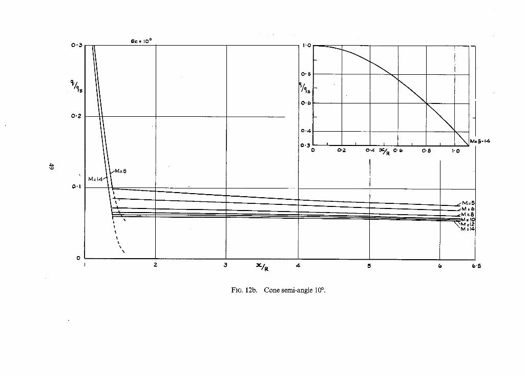
0 . 3

O-Z

Q . !

O

OC = IO °

0"2 I I

0..4. ~ / R 0"~o

\ 0.8, i 'O

IVi=5- I,~

l

_ _ _ . . . ~ M = 5 ~ M - - 6 ..---_._,:M = 8

z ~ / ~ ,a. 6 .S

FIG. 12b. Cone semi-angle 10 °.

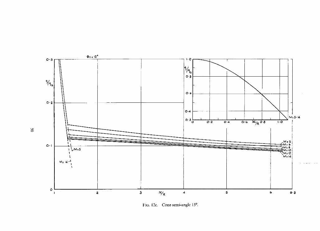
0 " 3

0 " 2

Or..: 15 e 0

t'5 8

,b

4

5 0 0 " 2

I 0 ' 4

i i o.~o ~c/R 0.8

• M:5-J4.

I . O

0 . I ~ . M : 5

I I

M= 14 -A I I

¢o

M ~ I 4

6"5

FIG. 12C. Cone semi-angle 15 °.

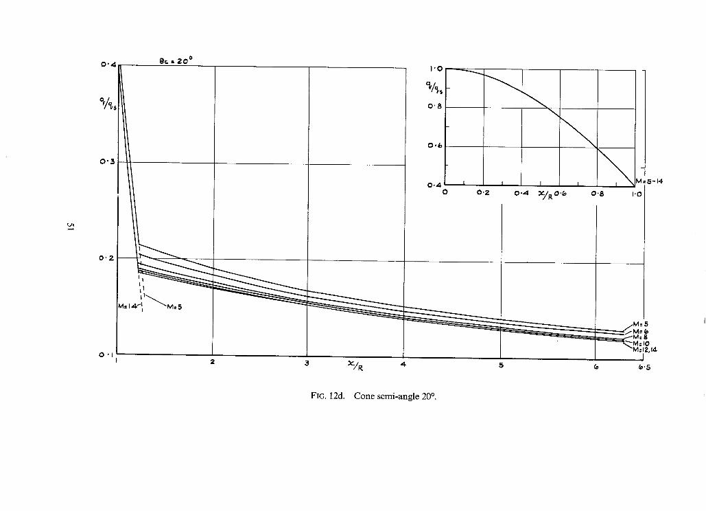
0 " 4

%,

0 " 3 ~ .

0"2

0 ' (

ec. = 2 0 °

Vl; 14~11 " " M = 5

I '0

0"8

0.6

0.4 I 0

\

I I I

o.z o . 4 ~ / a o,(o

3 5

o.8 i.o

M.-5

~ M = 8

~M.'12,14. I

~ '5

FIG. 12d. Cone semi-angle 20 °.

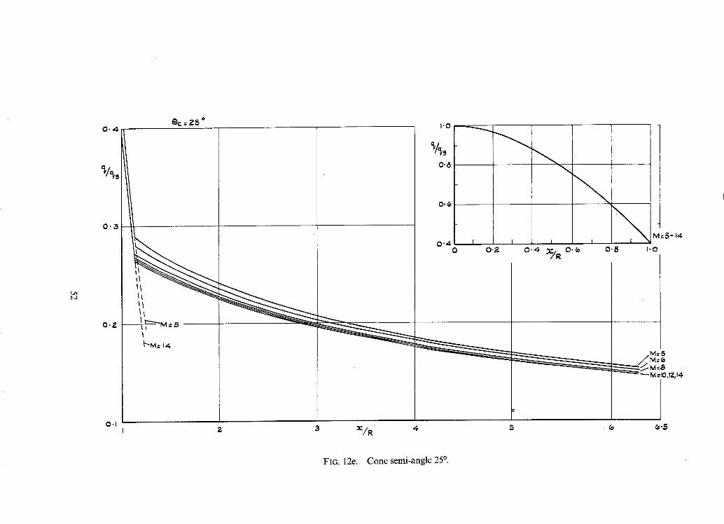
0 . 4

0 , 3

I'0 - ~

)'8

,.4, I

0 0.~, I I

0-4.

\ M : 5 - 14

0'8 I.o

0 . £ f - - - - -~ - - : . ~

0.1

II

I V-M= I~,

2 ~ / R 4

M--5

M=EI,IZjI4

(o ~ ' 5

FIG. 12e. Cone semi-angle 25 °.

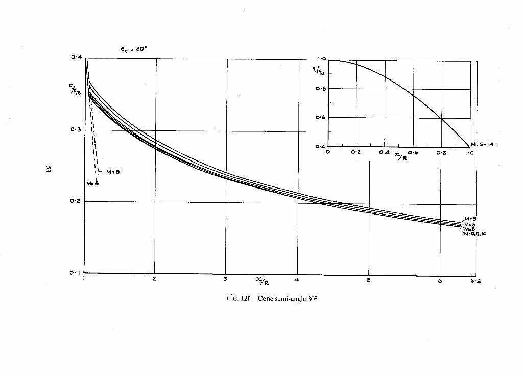
0 , 4

0"3

0 ' 2

0"1

@¢ : ~ O °

M:I~,

I '0

0"8

0"6

0.4 I 0 O'Z

I

0 ' = " ~ / ' R O ' ( o

I I 0%

• vI=~5-14.

l 'O

~ - M " 6

M=IO~I2j 14

FiG. 12f. Cone semi-angle 30 °.

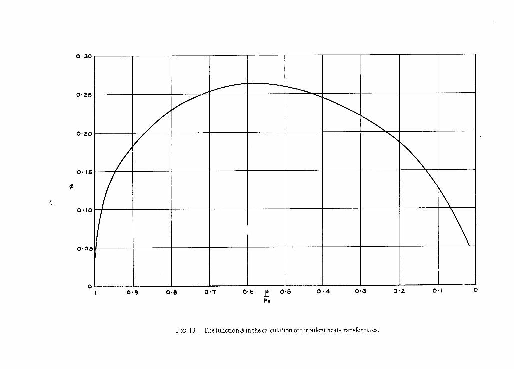
0 " 3 0

0"?-5

O'ZO

0 - 1 5

0 - 1 0

0 , 0 5

0 I

Y

o , 5 o . 4 o . ~ o . z o . i o 0 . 9 o . 8 a . 7 o.~0 _~ P~

FIG. ] 3. The function ~b in the calculation of turbulent heat-transfer rates.

L~ L~

I 0 0

I 0

2

0 < U~

Id

0 z

0"I

0 ' 0 1 " 0

STAGNATION HEATING L.E~S THAN MAXIMUM TURBULENT RATE.8.

J t

8TACNATION HEATING GRE,~TER THAN MAXIMUM TURBULENT RATF.~.

ZO,O00 4 0 , 0 0 0 &O, O00 8 o , 0 0 0 I00 ,000 IZO~O00 140

AL.TITIADF.., F'T. 000 ;bO, OO0 180,000

FIG. 14. Maximum nose radius for stagnation heating rates to exceed maximum turbulent rates.

ZOO, 0 0 0

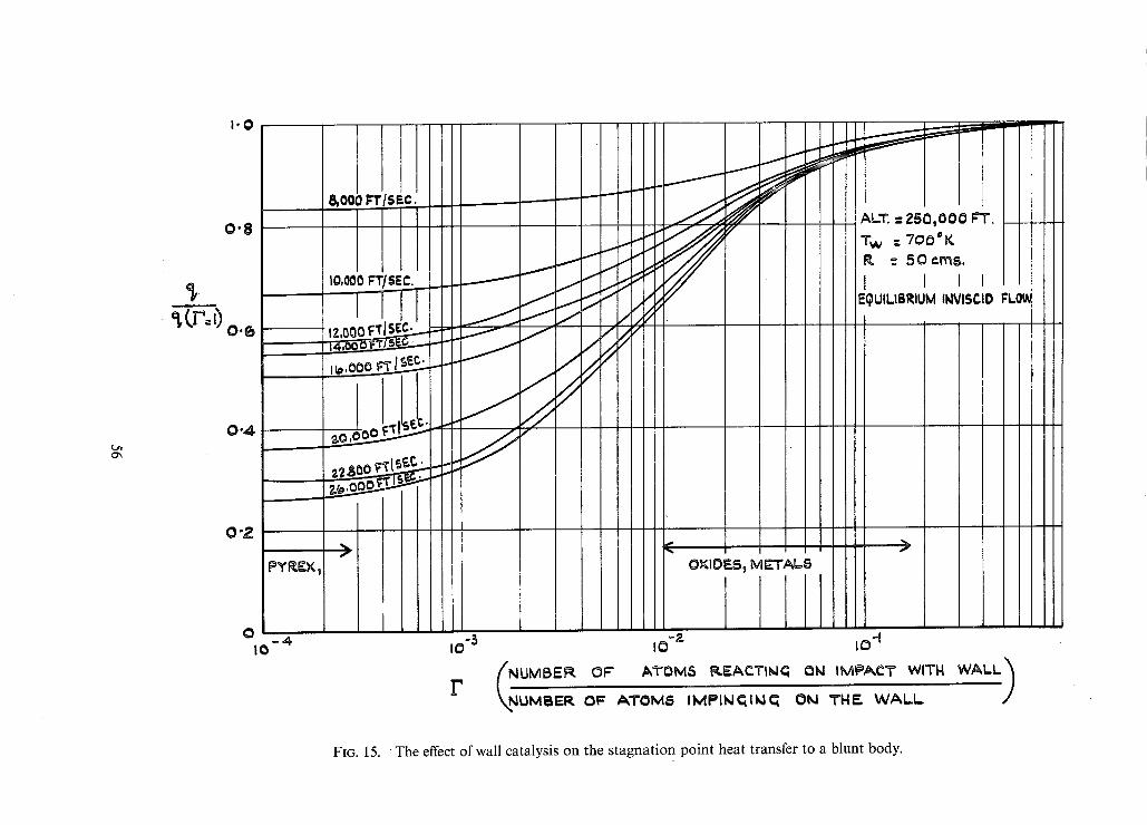
1.0

0 .8

~(,r-0 O'6

L.h

0"4

0"2.

O -,4. I0 10-3 i0 -z 10 °l ('NUMBE~ oF ,,,TOMS ~ E A c ' r ~ oN ~MP~c'r w,'rN

r k , ~ o~ ATOMS , M P l N ~ , ~ O~ THE WAL.-

WALL)

FIG. 15. T h e effect of wall catalysis on the stagnation point heat transfer to a blunt body.

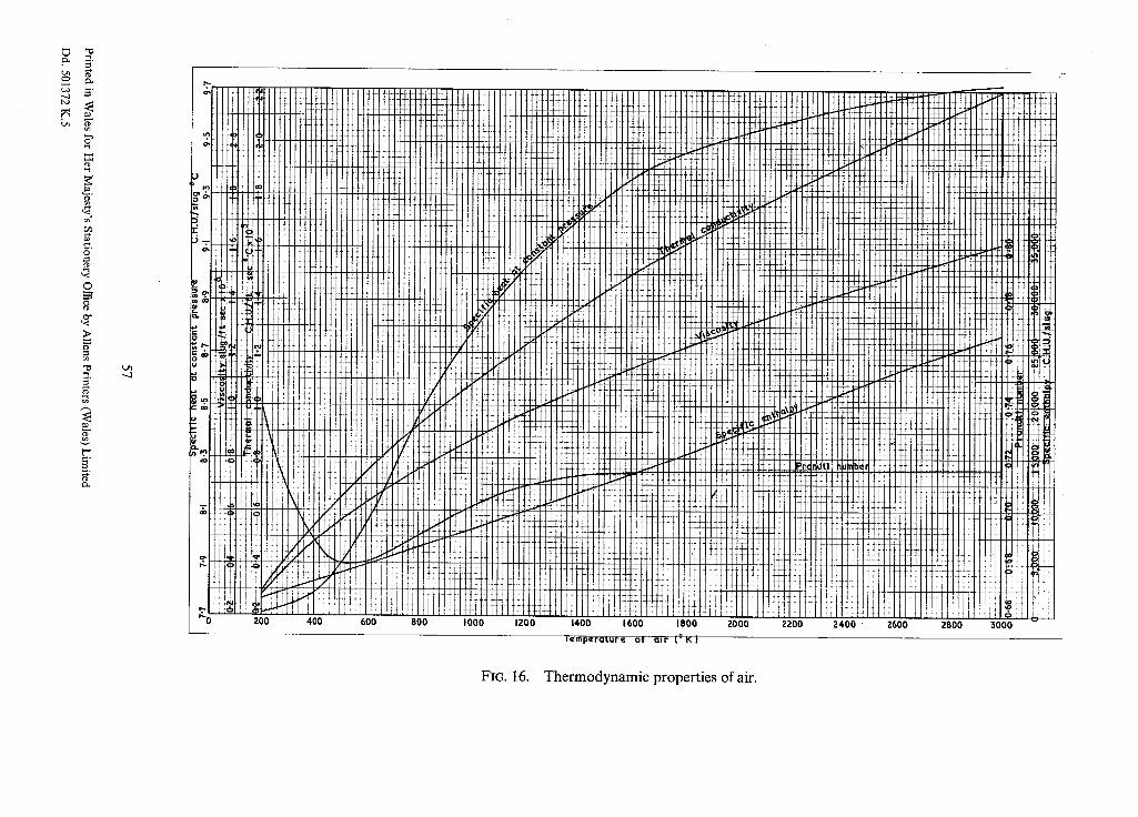
o-

c~

o

©

o"

>

IIHH IAtHImltlIlfllllfttlItt i ttt!!t l I~t~Tttttt~Htt-IttftffH ttt~HfHttt

i T ~ ~ i .1 ! ~ ~ ~ ~ ~ i ~ ~ ~ I ~ Hilt ii~t! ! ~ I ~ ~ ! H ! l l Ill tit-tilt t4t!tt!Htttt! t t i i t i ! t ~ t tttttltiitlttt]tH!!tttI7 t

200 400 600 800 I000 I;'00 1400 1600 1800 ZOO0 2200 :)400 2600

Temperature at air {0 K)

t]tttTtH~IN

1~ t~

it t liit~i ~ i i ;'800 3000

FIG. 16. Thermodynamic properties of air.

R. & M. No. 3637

((~ Crown copyright 1970

Published by [|liP, MAJESTY'S SIA'IIONtRY OFFICE

To be purch~ised from 49 ttigh Holborn, LondonWC1 6t tB 13a Castle Street, [idiilburgh EH2 3AR 109 St Mary Street, Cardiff CF1 l JW

Brazannose Streel, Manchester M60 8AS 50 Fairfax Street, Bristol BS1 3DE 258 Broad Street, Birmingham I

7 Linenhall Street, Belfast BT2 8AY or through any bookseller

R. & NL No. 3637

SBN 11 470337 X

Documents

Estimation of Heat Transfer to Flat Plates, Cones and Blunt Bodies