Zukurov et al. Algorithms Mol Biol (2016) 11:2 DOI 10.1186/s13015-016-0064-x

SOFTWARE ARTICLE

Estimation of genetic diversity in viral populations from next generation sequencing data with extremely deep coverageJean P. Zukurov1, Sieberth do Nascimento‑Brito2,5, Angela C. Volpini6* , Guilherme C. Oliveira6, Luiz Mario R. Janini1,2 and Fernando Antoneli3,4

Abstract

Background: In this paper we propose a method and discuss its computational implementation as an integrated tool for the analysis of viral genetic diversity on data generated by high‑throughput sequencing. The main motivation for this work is to better understand the genetic diversity of viruses with high rates of nucleotide substitution, as HIV‑1 and Influenza. Most methods for viral diversity estimation proposed so far are intended to take benefit of the longer reads produced by some next‑generation sequencing platforms in order to estimate a population of haplotypes which represent the diversity of the original population. The method proposed here is custom‑made to take advan‑tage of the very low error rate and extremely deep coverage per site, which are the main features of some neglected technologies that have not received much attention due to the short length of its reads, which precludes haplotype estimation. This approach allowed us to avoid some hard problems related to haplotype reconstruction (need of long reads, preliminary error filtering and assembly).

Results: We propose to measure genetic diversity of a viral population through a family of multinomial probability distributions indexed by the sites of the virus genome, each one representing the distribution of nucleic bases per site. Moreover, the implementation of the method focuses on two main optimization strategies: a read mapping/alignment procedure that aims at the recovery of the maximum possible number of short‑reads; the inference of the multinomial parameters in a Bayesian framework with smoothed Dirichlet estimation. The Bayesian approach pro‑vides conditional probability distributions for the multinomial parameters allowing one to take into account the prior information of the control experiment and providing a natural way to separate signal from noise, since it automati‑cally furnishes Bayesian confidence intervals and thus avoids the drawbacks of preliminary error filtering.

Conclusions: The methods described in this paper have been implemented as an integrated tool called Tanden (Tool for Analysis of Diversity in Viral Populations) and successfully tested on samples obtained from HIV‑1 strain NL4‑3 (group M, subtype B) cultivations on primary human cell cultures in many distinct viral propagation conditions. Tanden is written in C# (Microsoft), runs on the Windows operating system, and can be downloaded from: http://tanden.url.ph/.

Keywords: Viral diversity, Bayesian inference, Dirichlet distribution

© 2016 Zukurov et al. This article is distributed under the terms of the Creative Commons Attribution 4.0 International License (http://creativecommons.org/licenses/by/4.0/), which permits unrestricted use, distribution, and reproduction in any medium, provided you give appropriate credit to the original author(s) and the source, provide a link to the Creative Commons license, and indicate if changes were made. The Creative Commons Public Domain Dedication waiver (http://creativecommons.org/publicdomain/zero/1.0/) applies to the data made available in this article, unless otherwise stated.

Open Access

Algorithms forMolecular Biology

*Correspondence: avolpini@cpqrr.fiocruz.br 6 Genomics and Computational Biology Group, Centro de Pesquisas René Rachou (CPqRR), Fundação Oswaldo Cruz (FIOCRUZ), Belo Horizonte, BrazilFull list of author information is available at the end of the article

Page 2 of 15Zukurov et al. Algorithms Mol Biol (2016) 11:2

BackgroundViruses with RNA genomes are recognized to generate particularly mutant-rich populations called quasispecies. The genetic heterogeneity characteristic of viral qua-sispecies is largely due to high mutational rates combined with an elevated population size [1]. Human immunode-ficiency virus 1 (HIV-1), as an example, has a mean sub-stitution rate of order 10−5 per nucleotide position [2]; that is by far higher than those of cellular organisms [3, 4] and assures a constant viral mutant production.

Next-generation sequencing (NGS) platforms have been used mainly for the de novo sequence assembly of viruses. However, more recently, new interest arose in re-sequencing known virus genomes using NGS to study the diversity of viral populations. All NGS platforms pro-duce short segments of DNA, called reads, which pro-vide only imperfect and incomplete information about the structure of the viral population. Sequencing errors and length of reads are factors that must be taken into account in the analysis of data obtained from NGS viral quasi-species. In addition, reverse transcription and PCR amplification are procedures prone to errors. The impact of these errors on studies of viral diversity could be huge (see below), therefore one wants to separate true genetic variation from methodological noise and if both are of the same order of magnitude the task becomes virtually impossible.

Regarding the development of tools to estimate genetic diversity of viral populations (total number of genetic characteristics in a viral ensemble), the most commonly used NGS platforms are the 454™ (Life Sciences/Roche)—since Roche’s announced in October 2013 it will shut-down the 454™ platform [5] its use has been fading—and the Illumina™ (Solexa), mainly due to their capacity to produce longer reads. The ability to produce relatively long sequences favors the development of methods aim-ing at the haplotype (the genetic variants in a viral popula-tion) reconstruction of the representative viral particles in population [6, 7]. However, the propagation of sequencing errors is a serious problem in these methods, requiring the development of procedures for error correction, which my introduce unwanted biases. In general, the fraction of wrong reads increases with the error rate per base and the average length. The expected proportion of reads with at least one sequencing error as a function of the error rate per base ε and the average length L of reads is given by the relation 1 − (1 − ε)L [8]. As the estimated error rate of 454™ is about 0.1–0.5 % and Illumina™ error rates are in the range of 0.1–1 % [9], with an average length of reads from 400 bp up to 1000 bp, the proportion of reads with at least one error is in the range 35–90 %. The platform SOLiD™ (Life Technologies), for instance, is at the other end of the spectrum. With reads of short length, of at

most 50 bases (the main limitation for the construction of haplotypes) and estimated error rate of 0.06 % [9], the proportion of reads with at least one error is around 2 %. Recently, a different solution to the problem of sequenc-ing errors has been proposed [10], based on the develop-ment of high-fidelity sequencing protocols [11].

A more serious challenge associated with the assembly of all possible haplotypes is the NP-hardness of the cor-responding combinatorial optimization problems [12]. In fact, some approximate solution must be employed and a crucial hindering factor is the ratio between the size of the reads and the size of the genomic region being recon-structed. For instance, it has been reported [10] that short read lengths (less than 100 base pairs) dramatically inhibit reconstruction of genomes with more than 3400 bp, evi-denced by the failing to produce any complete genome. Another major shortcoming of all existing methods for haplotype reconstruction is that they are unable to handle large insertions or deletions (indels), only very recently this problem seems to have been overcome [13].

As mentioned before, the ability of the other NGS plat-forms to produce relatively long sequences have been a great stimulus to the development of methods for build-ing haplotype representatives of viral particles in the population and the vast majority of softwares for viral diversity estimation that have been proposed until very recently adopt this perspective [6]. The aim of this work is to propose a different approach to measure genetic diver-sity that does not demand any kind of length assumption on the short reads, but takes advantage of the low error rate and the high depth of coverage per site inherent to some NGS platforms. Therefore, we shall considerably depart from the most traditional developments aim-ing at haplotype reconstruction, since not every one has access to the NGS platforms appropriate for that pur-pose. Indeed, although the short length of the reads pro-duced by these platforms essentially hinders haplotype reconstruction, it is possible to measure genetic diversity through probability distributions along the genome (one per site) and this approach is enhanced by the highly deep coverage provided by these NGS platforms.

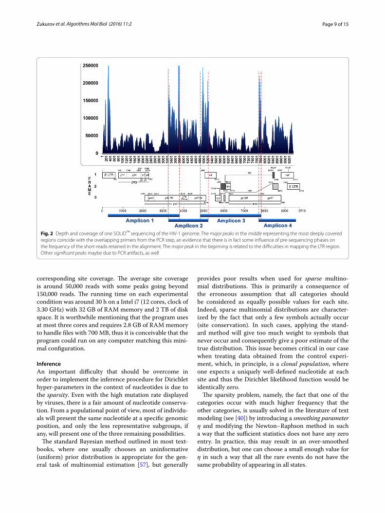
A recent study [14] comparatively assessed the per-formance of some NGS platforms (including 454™ and Illumina™) and reported an average (range) cover-age of  ~23,000 reads (5000–47,000) for the Illumina™ and  ~7000 reads (2000–22,000) for the 454™. We used the SOLiD™ platform and were able to achieve an aver-age (range) coverage of ~50,000 reads (10,000–150,000), for instance (see Fig. 2). In addition, the low error rate of 0.06 % provided by the SOLiD™ platform virtually elimi-nates the necessity of any error correction procedure. Instead, we use the estimated probability distributions to separate signal from noise.

Page 3 of 15Zukurov et al. Algorithms Mol Biol (2016) 11:2

The first step in nucleotide sequence analysis is read mapping/alignment. This is important for many bioin-formatics applications, as exemplified by nucleic acid conformational structure prediction and phylogeny studies [15, 16]. As expected, this is also an important aspect for NGS data analysis involving all the different platforms as Ion Torrent™ (Life Technologies), SOLiD™, 454™ and Illumina™ [17, 18] and others. Nowadays, users can choose from a panoply of tools for map-ping and indexing NGS reads, available on-line and for download. MAQ (Mapping and Assembly with Quali-ties) [19], BWA (Burrows–Wheeler alignment tool) [20], BFAST (Blat-like fast accurate search tool) [21], Bowtie [22] and MOSAIK [23] are examples of such alterna-tives. Those tools allow the fast mapping and alignment of reads belonging to genomes up to 109 bp in length [20, 24, 25].

After the read mapping is finished, the following step consists in the choice of a strategy for statistical infer-ence. There is a wide variety of methods depending on the scope and the goals of the analysis: (1) consensus gen-eration, (2) single nucleotide variant (SNV), also called single position diversity estimation, (3) local diversity esti-mation and (4) read graph-based haplotype reconstruc-tion, also known as global diversity estimation, see [8, 26] for a thorough explanation of these concepts. Exist-ing tools for genetic diversity evaluation of viral NGS sequences, intended for 454™ and Illumina™ platforms [8, 26–33], are based on several techniques aiming at haplotype reconstruction [30, 34–39].

In order to estimate the genetic diversity without resorting to haplotype reconstruction, we propose to represent the genetic diversity of a sample population through a family of multinomial probability distributions indexed by the sites of the virus genome, each one repre-senting the distribution of nucleic bases per site. Moreo-ver, the inference of the multinomial parameters is done in a Bayesian framework using smoothed Dirichlet esti-mation inspired by a method for modeling text data [40].

Inference of multinomial parameters is a challenging problem in statistics. For the simplest case, i.e., the Ber-noulli model or binomial estimation, the history traces back to Thomas Bayes [41]. Karl Pearson [42] called this seemingly simple problem the “fundamental prob-lem of practical statistics”. In the frequentist context the problem is called “interval estimation of a binomial proportion” and there is a textbook solution based on a confidence interval for this problem, which however has several drawbacks [43]. In both frameworks the fre-quency of occurrence of a category plays a crucial role, leading to the “sufficient statistics” in the Bayesian con-text and the “estimator of proportion in a sample” in the frequentist context.

The choice of a Bayesian framework is motivated by two features that are not present in the frequentist frame-work: (1) it allows one to obtain conditional (posterior) probability distributions for the multinomial parameters and thus interpret the point estimates as probabilities—this interpretation conceptually incorrect when applied to pure relative frequencies (which is not the same thing as adopting frequentist framework)—even though the law of large numbers implies that they converge to the point estimates obtained from the Dirichlet distribu-tions when the number of observations goes to infin-ity; (2) on may take into account the prior information of the control experiment (whose genome sequence is known) within the inference of a posterior experimen-tal condition by means of Bayes’ formula and thus relate two temporally connected events. Finally, it provides a natural way to separate signal from noise through cred-ible (or Bayesian confidence) intervals—another problem with the use of pure relative frequencies is that it is not possible to associate “error bars” to them. Therefore, in our aproach, the errors introduced during the sequenc-ing process are not filtered before the inference, but after it, when we identify the relevant signal—this allows us to avoid the drawbacks of preliminary error filtering [10, 44].

In summary, we sought to build an analysis platform suitable to address the problem of estimation of the pop-ulational genetic diversity of RNA viruses. Due to high mutational rates and accelerated replicative kinetics, RNA viruses constitute ensembles of variants, known as quasispecies, which, instead of a collection of viral par-ticles, behave as a single and coherent organism which is act on by the host’s pressures [45]. Furthermore, our mathematical and computational approach allows for a better understanding of virtually all the viral diversity present in a clinical sample. By saying this, we mean that our method gives the user an idea about the real structure of a viral population contained in a clinical sample at a given time. When a quasispecies population is challenged by selective pressures, it responds as a sole organism due to the mutational link between the genetic variants it contains. Following this train of thoughts, at any given moment this distribution of mutants may bear variants with resistance mutations (which could minimize thera-peutic success) or virus with genomic compositions that were sufficiently close to therapeutical resistance. In this manner, as far as clinical applications are concerned, our method offers an opportunity to the clinician to observe the entire viral mutational landscape in a clinical sample. This comprehensive view could help the clinician when deciding the best therapeutic approach.

Based on the aforementioned assumptions and that a NGS platform generates an extremely high number of

Page 4 of 15Zukurov et al. Algorithms Mol Biol (2016) 11:2

reads of short length allowing for a deep and extensive cov-erage of the data, and with a very low error rate, we propose an approach to the estimation of genetic diversity of viral populations that does not make requirements on the form of the sequenced data (such as [10], which works only with Illumina™) and does not assume any statistical model for filtering errors [8]. Despite its apparent mathematical and computational involvement the approach proposed here is one of the simplest conceptually correct possible choices.

Unfortunately, we could not find any other method or software in the literature, which uses a similar form to represent the viral genetic diversity as a family of distri-butions indexed by the genome and does not need suf-ficiently long reads—all proposals in the literature that we were able to find are aimed at haplotype reconstruc-tion and require longer reads (more than 100 bases). Any attempt to make comparison between such different approaches would be misleading, therefore it is not our aim here to make the point if the method presented here is an improvement over (non-)existing similar ones. In fact, we believe that the approach proposed here should not be considered alternative or rival, but complemen-tary, to haplotype reconstruction.

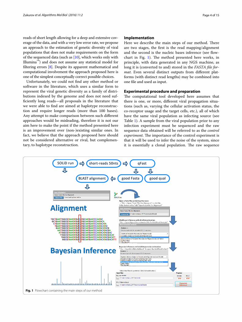
ImplementationHere we describe the main steps of our method. There are two stages, the first is the read mapping/alignment and the second is the nucleic bases inference (see flow-chart in Fig.  1). The method presented here works, in principle, with data generated in any NGS machine, as long it is (converted to and) stored in the FASTA file for-mat. Even several distinct outputs from different plat-forms (with distinct read lengths) may be combined into one file and used as input.

Experimental procedure and preparationThe computational tool developed here assumes that there is one, or more, different viral propagation situa-tions (such as, varying the cellular activation status, the co-receptor usage and the target cells, etc.), all of which have the same viral population as infecting source (see Table 1). A sample from the viral population prior to any infection experiment must be sequenced and the raw sequence data obtained will be referred to as the control experiment. The importance of the control experiment is that it will be used to infer the noise of the system, since it is essentially a clonal population. The raw sequence

Fig. 1 Flowchart containing the main steps of our method

Page 5 of 15Zukurov et al. Algorithms Mol Biol (2016) 11:2

data obtained from samples extracted from infected cells, after a fixed number of replication cycles, will be collec-tively called experimental conditions.

Raw sequence data from the sequencing must be treated according to the standard procedures of the spe-cific NGS platform [46] up to the generation of FASTA files, which are the standard type of input file adopted in our implementation.

The data used in this paper for testing the method is the subject of another publication [47], where the details of the experiments and the biological implications to the HIV replication are discussed. The method and the results described here do not depend on the experimen-tal details and the results reported in [47].

Read mapping/alignmentThe main goal of this step is the mapping of reads with 50 nucleotides or more originating from the NGS platform to a database of reference sequences. The database may con-tain several sequences, which must be aligned amongst themselves. The read mapping is performed using a local executable of BLAST [48]. The criteria for retaining the reads are the following: (1) it must align at least 45 nucleo-tides and (2) have the lowest e value score. A first align-ment attempt is made with sequences from reads in the forward sense; in case of no match, a second attempt with the reverse complementary sequence is performed. More-over, since we are using several references, the output can, in principle, display the same number of matches as there are reference sequences. The criteria for the selection of

the most suitable alignment option are the following (in this order): (1) the lowest e value score and (2) the lowest Hamming distance from the consensus sequence obtained from of the sequencing of the control experiment. The alignment strategy described above is set as default, but the user, according to some specific purposes or simply for increasing processing speed, can change some of its parameters. Finally, it is possible to create suitable refer-ence databases for specific research purposes.

Nucleic base estimationThe probability distributions of nucleic bases (A, T, C, G) at each position of the genome are estimated from the aligned data. In this respect, our approach may be clas-sified as a diversity estimation in single positions. The idea is that at each position in the genome the probabil-ity distribution is given by a multinomial distribution, determined by four probabilities (pA, pT, pC, pG) satisfy-ing pA + pT + pC + pG = 1. These conditional probabili-ties represent the fraction of the population that has each of the four associated nucleic bases at the corresponding site given the observed sequence data. Thus, one has a family of multinomial probability distributions indexed by the sites of the genome, where at each position the four probabilities (pA, pT, pC, pG) should be estimated from the data.

The Bayesian framework for the inference of categori-cal data is based on the notion of conjugate prior, which in the case of categorical data is given by the Dirichlet distributions [49, 50]. A Dirichlet distribution is char-acterized by a n-tuple of positive numbers α =  (α1,…, αn) called hyper-parameters—however, unlike the multinomial parameters that must sum to one, the hyper-parameters are unconstrained. In our case, the Dirichlet distribution of each site is parametrized by the quadruple (αA, αT, αC, αG). The fact that the Dir-ichlet distribution is the conjugate prior of the multi-nomial distribution amounts to saying that the Bayes’ formula for the posterior distribution takes a very sim-ple form in terms if the hyper-parameters: if (α1,…,αn) is a vector of hyper-parameters of a Dirichlet prior dis-tribution and the counts of each of the k categories in an experiment are (c1,…, cn) then the posterior distribu-tion is also a Dirichlet distribution with hyper-param-eters (α1  +  c1,…, αn  +  cn). Within this context, the first step in the estimation of the probability distribu-tions of nucleic bases consists in using the sequenced data from the control experiment as the input for the determination of prior hyper-parameters. Then, in the second step, one considers this distribution together with the sequenced data form the experimental condi-tions one uses Bayes’ formula to compute the posterior hyper-parameters.

Table 1 Summary of sequence data analyzed

The first column lists all the experimental conditions and the control experiment that where sequenced, the second column (Reads) displays the number of reads sequenced in each condition, the third column (Nucl.) displays the number of nucleotides in each condition, the fourth column (Mapped) displays the percentage of reads that have been mapped and the fifth column (Time) displays the time elapsed in each mapping procedure

Sequenced data Reads Nucl. Mapped (%)

Time (hour)

HIV1—non‑stimulated CD4/R5

1.11 × 107 5.53 × 108 91.81 34.88

HIV2—stimulated CD4/R5 1.04 × 107 5.19 × 108 90.84 34.18

HIV3—non‑stimulated CD4/X4

1.10 × 107 5.50 × 108 91.22 29.05

HIV4—stimulated PBMC/X4 9.41 × 106 4.71 × 108 91.14 13.63

HIV5—stimulated PBMC/R5 1.14 × 107 5.73 × 108 90.49 24.09

HIV6—non‑stimulated PBMC/X4

1.12 × 107 5.62 × 108 91.42 27.54

HIV7—non‑stimulated PBMC/R5

1.19 × 107 5.94 × 108 93.27 15.34

HIV8—control (pNL4‑3kfs) 1.01 × 107 5.05 × 108 93.10 30.14

Total 8.65 × 107 4.33 × 109 91.67 208.85

Page 6 of 15Zukurov et al. Algorithms Mol Biol (2016) 11:2

A n-dimensional Dirichlet distribution is defined in by a smooth probability density function on the set Δ of n-dimensional multinomial distributions, which is para-metrized as �n = {(p1, . . . , pn−1) : p1 + · · · + pn−1 ≤ 1}, here n is the number of distinct categories (states) that can observed and pk is the probability of observing the k-th category, for k = 1,…, n with pn = 1− p1 + . . .+ pn−1. The Dirichlet probability density function is given by

where B(α) is a normalizing factor defined in terms of the gamma function Γ as

for a vector α =  (α1,…, αn). Note that the choice (α1,…, αn) = (1,…, 1) gives the uniform distribution (the flat or uninformative prior) on Δn with mass equal to the vol-ume of �n : B(1, . . . , 1)= 1/Ŵ(n)= 1/(n−1)!.

The Dirichlet hyper-parameters associated to the sequenced data from the control experiment represent the “noise” of the system and can be obtained by maxi-mum likelihood estimation (MLE) through the Newton–Raphson method [51]. The log-likelihood function g of the Dirichlet distribution is given by g = N log L and

where N is the sample size and log pk = 1/N∑

j log pjk (j = 1,…, N, k = 1,…, n) is called the sufficient statistics associated to a sample of n-categorical vector obser-vations {p1,…, pN} of sample size N. Thus each vector pj = (pj1,…, pjn) has n components, each component pjk is the frequency of the kth category at the jth sample.

The Newton–Raphson method for the maximum likeli-hood estimation of Dirichlet hyper-parameters amounts to the iteration of the following fixed-point scheme [49], which converges to the unique maximum value of g:

where αnew and αold are vectors of Dirichlet hyper-param-eters. The function ∇g(α) is the gradient vector (deriva-tive) of the log-likelihood function g, with components

Dir(p1, . . . , pn−1|α1, . . . ,αn) =1

B(α)

∏

k

pαk−1k

B(α) =

∏

k Ŵ(αk)

Ŵ

(

∑

k αk

)

log L(

α1, . . . ,αn∣

∣p1, . . . , pn)

= log Ŵ

(

∑

k

αk

)

−∑

k

log Ŵ(αk )+∑

k

(αk − 1) log pk ,

αnew = α

old +

[

H−1∇g](

αold

)

,

[∇g(α)]k = �

(

∑

k

αk

)

−�(αk)+ log pk ,

where Ψ =  (log Γ)′ is the digamma function. The func-tion H−1(α) is the inverse of the hessian matrix of the log-likelihood function g and the product (H−1∇g)(α) =  H−1(α)∇g(α) has components [(H−1∇g)(α)]k given by

where Ψ′ is the trigamma function (k, l = 1,…, n). Several suggestions for the initialization step (that is, the initial value of αold) of the iteration scheme described above have appeared in the literature [50, 52, 53]. The proposal of Ronning [53] is the most suitable for the modified iter-ation scheme adopted here.

Since we are dealing with a sparse estimation prob-lem in the sense that one of the categories occur with much higher frequency that the other categories, we shall employ the smoothed sufficient statistics defined by introducing a small parameter η and setting pjk = Mjk/M, where Mjk is the number of occurrences of the kth cate-gory at the jth sample, M is total number of observations at the jth sample and pjk = η if there is no occurrence of the kth category at the jth sample. The smoothing param-eter η acts as “background noise” representing sequenc-ing and PCR errors that can not be removed. However it can be suitably tuned in order to account for the true variability of the data. When this procedure is applied to the sequenced data from the control experiment (a “clonal” population) one would expect no diversity at all. However, that is not completely true and, in fact, even the sequenced data from the control experiment should dis-play some variability (mainly due to sequencing errors). The smoothing parameter η should be at same (or smaller than) of the order of magnitude of expected error rate ε. In the smoothed version of the Newton–Raphson itera-tion scheme, Ronning’s initialization step is given by set-ting αold = (η,…, η).

The sufficient statistics is computed by a simple re-sam-pling procedure [54, 55] in order to generate sequences of categorical observations from the raw sequenced data, by randomly sampling nucleotides form each aligned posi-tion. Here, the imperfect clonality of the sequenced data from the control experiment is useful, since it ensure that the re-sampled ensemble has some variability, which is consistent with having a small non-zero smoothing parameter. The re-sampling procedure has one parameter that can be adjusted by the user: the relative size of obser-vations given as a fraction 0 < z < 1 of the size C of the set of nucleotides covering the given site. If the number of

[(

H−1∇g)

(α)

]

k

=(

� ′(αk))−1((

∇g)

k

+

(

∑

l

(∇g)l

� ′(αk)

)

/

(

1

� ′(∑

l αl) −

∑

l

1

� ′(αl)

))

,

Page 7 of 15Zukurov et al. Algorithms Mol Biol (2016) 11:2

bases covering the given site is denoted by C then M = zC is the number of observations used to compute one sam-ple vector pj = (pj1,…, pjn) and the corresponding sample size N is given by (the integer part of ) the logarithm of the total number of all possible sample vectors:

Stirling’s formula gives the following approximation in terms of C:

For instance, for the default value of z, which is 80 %, one has a sample of size N ≈  0.7C, each sample vector computed from 0.8  M nucleotides. On the other hand, the value z =  50  % gives a sample of size N ≈  C, each sample vector computed from 0.5 M nucleotides.

Once the hyper-parameters of the prior distribu-tion are estimated, they must be used together with the sequenced data of the other experimental conditions in order to compute the hyper-parameters of the posterior distributions by Bayes’ formula, as a result, one obtains a family of Dirichlet probability distributions indexed by the genome of the organism for every sequenced experi-mental condition, including the control experiment.

In order to obtain point estimates of categorical prob-abilities per site for each experimental condition (pA, pT, pC, pG), one may use a central tendency measure of the corresponding Dirichlet distribution (see [49]). Let x = (x1,…, xn) be a random vector distributed according to a Dirichlet distribution with corresponding hyper-parameters (α1,…,αn) then the number s = α1 +⋯+ αn is called the concentration parameter of the corresponding Dirichlet distribution. It provides a measure of the “qual-ity” of the inference: the greater the value of s the better is the “precision” of the inference (see [49]). The mean value of x is

The maximum a posteriori (MAP) estimate, which is given by the mode of x, has become a very popular method of point estimation [10]. Moreover, the coordi-nates ‹‹xk›› of the mode of x may be directly calculated in terms of the hyper-parameters αk only when αk  >  1 (k = 1,…,n):

This is much simpler than the contrived expecta-tion–maximization (EM) approximate schemes usually employed to obtain the MAP estimate from a log-like-lihood function, in which case approximations are una-voidable, since this function is non-convex.

Note that both the mean ‹xk› and the mode ‹‹xk›› converge to the same value when the number of

N = [log Ŵ(C)− log Ŵ(zC)− log Ŵ((1− z)C)].

N ≈ C(

−z log z − (1− z) log (1− z))/

log 2.

�xk� = αk/s.

��xk�� = αk/(s − n).

observations goes to infinity. In particular, when the number of observed nucleic bases at certain site is very large then the relative frequencies of the different nucleic bases are very close to the values of the Dir-ichlet mean and mode.

Confidence values associated to the point estimates may be defined in terms of a dispersion measure of the corresponding Dirichlet distribution. The variance of x is given by

Since the marginal distribution of each xk is a one-dimensional Dirichlet distribution, also known as Beta distribution, the standard deviation of the mean σ(x)  =  square-root(Var(x)) may be used to construct Bayesian credible intervals about the expectation value.

The the standard deviation of the mean σ(xk) may be used to define credible intervals about the mode as well. Since the Beta distribution is unimodal, when all αk > 1 (k = 1,…, n), and has finite variance, a 3-sigma interval around the mean or the mode would provide about 95 % of confidence in the prediction (this is a general conse-quence of the Gauss-Vysochanskij-Petunin inequality, see [56]).

Finally, we should note that the inference procedure explained above is clearly not restricted to the case of four nucleotides (A, T, C, G), that is n = 4. It is trivial to modify it in order to account for insertions and deletions, or to work with codons and amino-acids.

Selection criteria and error filteringOnce the inference has been completed it is desirable to filter the errors and extract some subset of the data—for instance, most conserved sites, most variable sites, etc. In order to do so we have implemented two selection crite-ria based on simple quantities: (1) complementary prob-ability per site and (2) variational distance per site.

The complementary probability per site is defined as pcomp = 1 − max{pA, pT, pC, pG} and it depends only on the probability distribution of each site. It provides a measure of how much the distribution is concentrated in one state. For instance, if the complementary probability at a site is high it means that there was variation in the site prior to the experiment.

The variational distance per site is a positive number between 0 and 2 defined by vd =

∣

∣pA − p′A∣

∣ +∣

∣pAT − p′T∣

∣ +∣

∣pC − p′C

∣

∣ +∣

∣pG − p′G

∣

∣ , where (pA, pT , pC , pG) is the probability distribution per site of the control experiment and

(

p′A, p′T , p

′C , p

′G

)

is the probability distribution at the corresponding site of the experimental condition. It is a measure of the relative variation per site from the clonal population before and after the infection. If it is very low

Var(xk) = αk s − αk/

(

s2(s + 1))

.

Page 8 of 15Zukurov et al. Algorithms Mol Biol (2016) 11:2

at a site it means that the site did not undergo significant changes in relation to the sequenced data from the con-trol experiment.

The complementary probabilities and the variational distance can work as filters and the user must specify the thresholds for them. By using these two criteria in com-bination one may easily obtain some qualitative informa-tion about the behavior at a site.

An example of how to combine our method with any haplotype reconstruction procedure is the following. In a haplotype reconstructed population the fraction of a nucleic base X at a given position could be computed by summing the proportions of all haplotypes that have the nucleic base X at the given position. Using these propor-tions one can construct a family of distributions (fA, fT, fC, fG), with fA + fT + fC + fG = 1, per position. Since in prac-tice it is very difficult to obtain the low-frequent variants the variational distance between the distribution (fA, fT, fC, fG) and the distribution (pA, pT, pC, pG) can be used to estimate how far one is from having obtained all the vari-ants up to the lowest-frequent ones.

Another application, is to use the distributions (pA, pT, pC, pG) to generate a population of “random haplotypes” with the correct nucleic base distribution and compare with a population of reconstructed haplotypes in order to study the correlations between the sites.

Results and discussionThe method presented here was tested on samples obtained after the HIV-1 strain NL4-3 (group M, subtype B) cultivation on primary human cell cultures. Different viral propagation conditions were used—varying the cel-lular activation status, the co-receptor usage and the target cells. The pseudo-typed viruses produced in these experi-ments were able to perform exactly one round of the rep-licative cycle. As a whole, there were seven experimental conditions in addition to the control experiment (Table 1).

Experimental procedure and preparationThe experimental procedure was performed in accord-ance with the standard procedures of the NGS platform SOLiD™ [46], up to the generation of FASTA files, which are the input data of our computational tool. Standard Life Technologies guidelines were used during sample preparation and sequencing while using the SOLiD™ platform v. 3.0. The size of the FASTA files containing the reads of each condition is around 700 Mb, consisting of about 107 reads.

Read mapping/alignmentThe use of BLAST to perform the read mapping has two reasons: first the multiple reference sequences allowed by BLAST makes it advantageous for analysis of viral

populations classically described as quasispecies, since we can include several variant genomes belonging to the same phylogenetic branch, and second, it is easier to con-trol the parameters of the alignment and multi-threading inside our program.

We used a reference database composed by 1258 sequences, properly aligned, all representatives of HIV-1 epidemics, most of them belonging to major group (group M) and its subtypes A, B, C, D, F, G, H, J, K, and some of their recombinants (http://www.hiv.lanl.gov/content/sequence/HelpDocs/subtypes-more.html). Some of the sequences are of complete HIV-1 genomes while others represented virtually (more than 90  % complete) complete genomes. All sequences are available at NCBI/Genbank. The reference database also contains sequences from HIV-1 group O, SIVcpz and HIV-1 strain NL4-3 and is packaged together with the software.

Even though it is known that BLAST is not the fastest aligner when compared with next-generation aligners, we were able to achieve a reasonable speed and control by setting the parameters and implementing some opti-mizations. For instance, even though BLAST is capa-ble of identifying alignments in both the forward and the reverse complementary senses, we have found that manually doing this significantly increases the retrieval of reads—we had 15 % increase in the retrieval of reads. BLAST can be sensitive if the right parameters are cho-sen (small word size, in particular). It can find an align-ment of a 42-mer with a multiple mismatches and gaps. On the other hand, some next generation aligners may fail to find an alignment if a mismatch or gap (or more than one of these) occurs within the beginning of the read, as this portion is used as a seed. An important fea-ture of BLAST is that all alignments are returned. If a read has 1000 alignments, 1000 alignments are reported. Another advantage is the ability to perform sub-string alignments. Next generation aligners tend to be focused on aligning the entire read length. BLAST will find an alignment and report what position within the read that the alignment start and ends. Finally, BLAST is a more sensible treatment of N’s. Some of the next-generation aligners store bases in 2-bit format. Meaning they can only internally represent A, T, C, G. The solution is to randomly assign N’s to one of the other bases, a solution that some may find imperfect.

For each experimental condition, comprising the align-ment of around 107 reads of 50 bases against 103 HIV-reference sequences with 104 sites each, we were able to map around 90 % of the reads, since the estimated frac-tion of reads with at least one error is around 2  %, we have achieved an almost optimal retrieval of reads.

For instance, Fig. 2 shows the result of the alignment of the sequenced data from the control experiment and the

Page 9 of 15Zukurov et al. Algorithms Mol Biol (2016) 11:2

corresponding site coverage. The average site coverage is around 50,000 reads with some peaks going beyond 150,000 reads. The running time on each experimental condition was around 30 h on a Intel i7 (12 cores, clock of 3.30 GHz) with 32 GB of RAM memory and 2 TB of disk space. It is worthwhile mentioning that the program uses at most three cores and requires 2.8 GB of RAM memory to handle files with 700 MB, thus it is conceivable that the program could run on any computer matching this mini-mal configuration.

InferenceAn important difficulty that should be overcome in order to implement the inference procedure for Dirichlet hyper-parameters in the context of nucleotides is due to the sparsity. Even with the high mutation rate displayed by viruses, there is a fair amount of nucleotide conserva-tion. From a populational point of view, most of individu-als will present the same nucleotide at a specific genomic position, and only the less representative subgroups, if any, will present one of the three remaining possibilities.

The standard Bayesian method outlined in most text-books, where one usually chooses an uninformative (uniform) prior distribution is appropriate for the gen-eral task of multinomial estimation [57], but generally

provides poor results when used for sparse multino-mial distributions. This is primarily a consequence of the erroneous assumption that all categories should be considered as equally possible values for each site. Indeed, sparse multinomial distributions are character-ized by the fact that only a few symbols actually occur (site conservation). In such cases, applying the stand-ard method will give too much weight to symbols that never occur and consequently give a poor estimate of the true distribution. This issue becomes critical in our case when treating data obtained from the control experi-ment, which, in principle, is a clonal population, where one expects a uniquely well-defined nucleotide at each site and thus the Dirichlet likelihood function would be identically zero.

The sparsity problem, namely, the fact that one of the categories occur with much higher frequency that the other categories, is usually solved in the literature of text modeling (see [40]) by introducing a smoothing parameter η and modifying the Newton–Raphson method in such a way that the sufficient statistics does not have any zero entry. In practice, this may result in an over-smoothed distribution, but one can choose a small enough value for η in such a way that all the rare events do not have the same probability of appearing in all states.

Fig. 2 Depth and coverage of one SOLiD™ sequencing of the HIV‑1 genome. The major peaks in the middle representing the most deeply covered regions coincide with the overlapping primers from the PCR step, an evidence that there is in fact some influence of pre‑sequencing phases on the frequency of the short‑reads retained in the alignment. The major peak in the beginning is related to the difficulties in mapping the LTR region. Other significant peaks maybe due to PCR artifacts, as well

Page 10 of 15Zukurov et al. Algorithms Mol Biol (2016) 11:2

Check points and validationThe method described here contains some heuristic deci-sions that should be supervised and properly validated. We have added a checkpoint at the read mapping stage and performed a validation of the smoothed Newton–Raphson method, attaining very good concordance with the expected results.

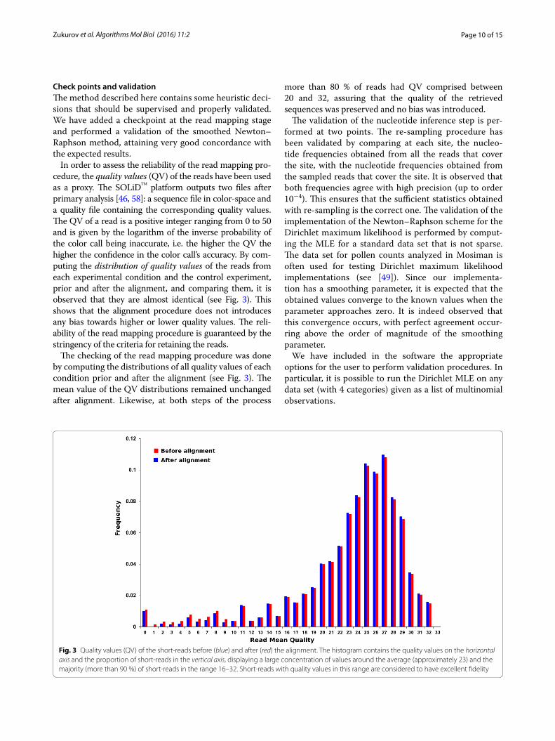
In order to assess the reliability of the read mapping pro-cedure, the quality values (QV) of the reads have been used as a proxy. The SOLiD™ platform outputs two files after primary analysis [46, 58]: a sequence file in color-space and a quality file containing the corresponding quality values. The QV of a read is a positive integer ranging from 0 to 50 and is given by the logarithm of the inverse probability of the color call being inaccurate, i.e. the higher the QV the higher the confidence in the color call’s accuracy. By com-puting the distribution of quality values of the reads from each experimental condition and the control experiment, prior and after the alignment, and comparing them, it is observed that they are almost identical (see Fig.  3). This shows that the alignment procedure does not introduces any bias towards higher or lower quality values. The reli-ability of the read mapping procedure is guaranteed by the stringency of the criteria for retaining the reads.

The checking of the read mapping procedure was done by computing the distributions of all quality values of each condition prior and after the alignment (see Fig.  3). The mean value of the QV distributions remained unchanged after alignment. Likewise, at both steps of the process

more than 80  % of reads had QV comprised between 20 and 32, assuring that the quality of the retrieved sequences was preserved and no bias was introduced.

The validation of the nucleotide inference step is per-formed at two points. The re-sampling procedure has been validated by comparing at each site, the nucleo-tide frequencies obtained from all the reads that cover the site, with the nucleotide frequencies obtained from the sampled reads that cover the site. It is observed that both frequencies agree with high precision (up to order 10−4). This ensures that the sufficient statistics obtained with re-sampling is the correct one. The validation of the implementation of the Newton–Raphson scheme for the Dirichlet maximum likelihood is performed by comput-ing the MLE for a standard data set that is not sparse. The data set for pollen counts analyzed in Mosiman is often used for testing Dirichlet maximum likelihood implementations (see [49]). Since our implementa-tion has a smoothing parameter, it is expected that the obtained values converge to the known values when the parameter approaches zero. It is indeed observed that this convergence occurs, with perfect agreement occur-ring above the order of magnitude of the smoothing parameter.

We have included in the software the appropriate options for the user to perform validation procedures. In particular, it is possible to run the Dirichlet MLE on any data set (with 4 categories) given as a list of multinomial observations.

Fig. 3 Quality values (QV) of the short‑reads before (blue) and after (red) the alignment. The histogram contains the quality values on the horizontal axis and the proportion of short‑reads in the vertical axis, displaying a large concentration of values around the average (approximately 23) and the majority (more than 90 %) of short‑reads in the range 16–32. Short‑reads with quality values in this range are considered to have excellent fidelity

Page 11 of 15Zukurov et al. Algorithms Mol Biol (2016) 11:2

Setting the smoothing parameter and separating the signal from the noiseThe complementary probability of an ideal clonal popu-lation is expected to be identically zero. However, in the smoothed inferential scheme proposed here it is expected that pcomp ≈ η. The choice of smoothing parameter does not affect the running time of the Newton–Raphson method; it affects the values of the estimated hyper-parameters. The effect is of the same order of magnitude of the smoothing parameter. This suggest the following guidelines for setting the smoothing parameter: η must be smaller that the error rate of the sequencing. Since the expected error rate ε in our case is around 6 × 10−4 a value of η = 10−5 is a reasonable choice for the smooth-ing parameter.

The concentration parameter s of the Dirichlet distribu-tions for the sequenced data from the control experiment is a measure of the quality of the inference: when s > 1 the inference may be considered meaningful. Sites with s ≤ 1 may be excluded from further analysis. Sites with low value of s may happen due poor coverage and total conser-vation (all reads with the same nucleotide at that position).

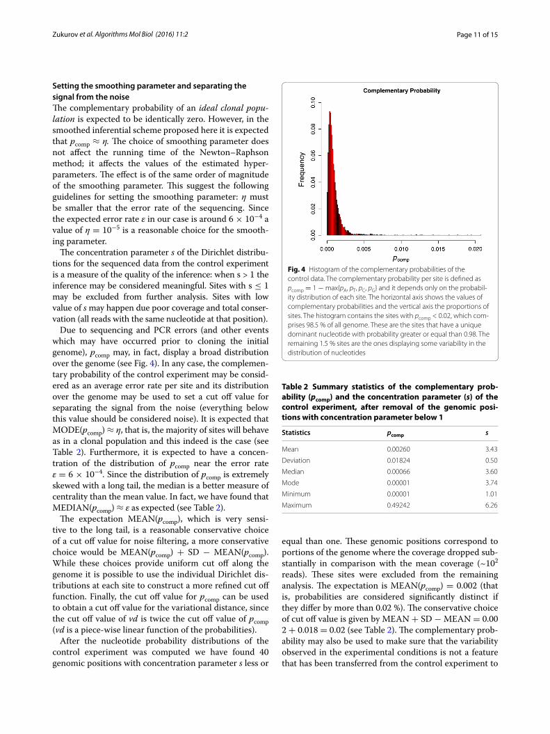
Due to sequencing and PCR errors (and other events which may have occurred prior to cloning the initial genome), pcomp may, in fact, display a broad distribution over the genome (see Fig. 4). In any case, the complemen-tary probability of the control experiment may be consid-ered as an average error rate per site and its distribution over the genome may be used to set a cut off value for separating the signal from the noise (everything below this value should be considered noise). It is expected that MODE(pcomp) ≈ η, that is, the majority of sites will behave as in a clonal population and this indeed is the case (see Table  2). Furthermore, it is expected to have a concen-tration of the distribution of pcomp near the error rate ε = 6 × 10−4. Since the distribution of pcomp is extremely skewed with a long tail, the median is a better measure of centrality than the mean value. In fact, we have found that MEDIAN(pcomp) ≈ ε as expected (see Table 2).

The expectation MEAN(pcomp), which is very sensi-tive to the long tail, is a reasonable conservative choice of a cut off value for noise filtering, a more conservative choice would be MEAN(pcomp)  +  SD −  MEAN(pcomp). While these choices provide uniform cut off along the genome it is possible to use the individual Dirichlet dis-tributions at each site to construct a more refined cut off function. Finally, the cut off value for pcomp can be used to obtain a cut off value for the variational distance, since the cut off value of vd is twice the cut off value of pcomp (vd is a piece-wise linear function of the probabilities).

After the nucleotide probability distributions of the control experiment was computed we have found 40 genomic positions with concentration parameter s less or

equal than one. These genomic positions correspond to portions of the genome where the coverage dropped sub-stantially in comparison with the mean coverage (~102 reads). These sites were excluded from the remaining analysis. The expectation is MEAN(pcomp) =  0.002 (that is, probabilities are considered significantly distinct if they differ by more than 0.02 %). The conservative choice of cut off value is given by MEAN + SD − MEAN = 0.002 + 0.018 = 0.02 (see Table 2). The complementary prob-ability may also be used to make sure that the variability observed in the experimental conditions is not a feature that has been transferred from the control experiment to

Fig. 4 Histogram of the complementary probabilities of the control data. The complementary probability per site is defined as pcomp = 1 − max{pA, pT, pC, pG} and it depends only on the probabil‑ity distribution of each site. The horizontal axis shows the values of complementary probabilities and the vertical axis the proportions of sites. The histogram contains the sites with pcomp < 0.02, which com‑prises 98.5 % of all genome. These are the sites that have a unique dominant nucleotide with probability greater or equal than 0.98. The remaining 1.5 % sites are the ones displaying some variability in the distribution of nucleotides

Table 2 Summary statistics of  the complementary prob-ability (pcomp) and  the concentration parameter (s) of  the control experiment, after  removal of  the genomic posi-tions with concentration parameter below 1

Statistics pcomp s

Mean 0.00260 3.43

Deviation 0.01824 0.50

Median 0.00066 3.60

Mode 0.00001 3.74

Minimum 0.00001 1.01

Maximum 0.49242 6.26

Page 12 of 15Zukurov et al. Algorithms Mol Biol (2016) 11:2

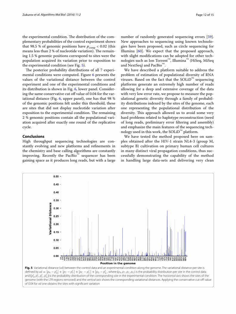
the experimental condition. The distribution of the com-plementary probabilities of the control experiment shows that 98.5 % of genomic positions have pcomp < 0.02 (this means less than 2 % of nucleotide variation). The remain-ing 1.5 % genomic positions correspond to sites were the population acquired its variation prior to exposition to the experimental condition (see Fig. 5).

The posterior probability distributions of all 7 experi-mental conditions were computed. Figure 6 presents the values of the variational distance between the control experiment and one of the experimental conditions and its distribution is shown in Fig. 6, lower panel. Consider-ing the same conservative cut off value of 0.04 for the var-iational distance (Fig. 6, upper panel), one has that 98 % of the genomic positions felt under this threshold, these are sites that did not display nucleotide variation after exposition to the experimental condition. The remaining 2 % genomic positions contain all the populational vari-ation acquired after exactly one round of the replicative cycle.

ConclusionsHigh throughput sequencing technologies are con-stantly evolving and new platforms and refinements in the chemistry and base calling algorithms are constantly improving. Recently the PacBio™ sequencer has been gaining space as it produces long reads, but with a large

number of randomly generated sequencing errors [59]. New approaches to sequencing using known technolo-gies have been proposed, such as circle sequencing for Illumina [60]. We expect that the proposed approach, with slight modifications can be adopted for other tech-nologies such as Ion Torrent™, Illumina™ (HiSeq, MiSeq and NextSeq) and PacBio™.

We have described a platform suitable to address the problem of estimation of populational diversity of RNA viruses. Based on the fact that the SOLiD™ sequencing platforms generate an extremely high number of reads allowing for a deep and extensive coverage of the data with very low error rate, we propose to measure the pop-ulational genetic diversity through a family of probabil-ity distributions indexed by the sites of the genome, each one representing the populational distribution of the diversity. This approach allowed us to avoid some very hard problems related to haplotype reconstruction (need of long reads, preliminary error filtering and assembly) and emphasize the main features of the sequencing tech-nology used in this work, the SOLiD™ platform.

We have tested the method proposed here on sam-ples obtained after the HIV-1 strain NL4-3 (group M, subtype B) cultivation on primary human cell cultures in many distinct viral propagation conditions, thus suc-cessfully demonstrating the capability of the method in handling large data-sets and delivering very clean

Fig. 5 Variational distance (vd) between the control data and an experimental condition along the genome. The variational distance per site is defined by vd =

∣

∣pA − p′A

∣

∣+∣

∣pT − p′T

∣

∣+∣

∣pC − p′C

∣

∣+∣

∣pG − p′G

∣

∣, where (pA , pT , pC , pG) is the probability distribution per site in the control data and

(

p′A , p′T , p

′C , p

′G

)

is the probability distribution of the corresponding site in the experimental condition. The horizontal axis shows the sites of the genome (with the LTR regions removed) and the vertical axis shows the corresponding variational distances. Applying the conservative cut‑off value of 0.04 for vd one obtains the sites with significant variation

Page 13 of 15Zukurov et al. Algorithms Mol Biol (2016) 11:2

results, suggesting that the software is a valuable tool for investigating the genetic diversity in viral popula-tions. We have successfully demonstrated Tanden’s capability of handling large data-sets and delivering very clean results, suggesting that the software is a valu-able tool for investigating the genetic diversity in viral populations as a complementary to some haplotype reconstruction method.

Availability and requirementsProject name: TandenProject web site: http://tanden.url.ph/Operating systems: WindowsProgramming language: Microsoft-C#License: free to all users under the LGPL licenseMinimum requirements: 4  GB RAM (16  GB recom-mended), 500 GB disk spaceThird party software used: BLAST  +  standalone for windows.(http://www.ncbi.nlm.nih.gov/blast/executables/blast+/LATEST/)

Authors’ contributionsJPZ: contributed to the statistical analysis, developed and implemented the software, drafted the manuscript; SNB: carried out the biological analysis, drafted the manuscript; ACV: contributed to NGS and bioinformatics analysis, drafted the manuscript; GCO: contributed to NGS bioinformatics analysis,

drafted the manuscript; LMRJ: conceived the statistical analysis, contributed to NGS and biological analysis, drafted the manuscript; FA: conceived the statisti‑cal analysis, developed and implemented the software, contributed to NGS and biological analysis, drafted the manuscript. All authors read and approved the final manuscript.

Author details1 Departmento de Medicina, Escola Paulista de Medicina (EPM), Universidade Federal de São Paulo (UNIFESP), São Paulo, Brazil. 2 Departamento de Micro‑biologia, Imunologia e Parasitologia, Escola Paulista de Medicina (EPM), Univer‑sidade Federal de São Paulo (UNIFESP), São Paulo, Brazil. 3 Departmento de Informática em Saúde, Escola Paulista de Medicina (EPM), Universidade Federal de São Paulo (UNIFESP), São Paulo, Brazil. 4 Laboratório de de Biocomplexidade e Genômica Evolutiva, Escola Paulista de Medicina (EPM), Universidade Federal de São Paulo (UNIFESP), São Paulo, Brazil. 5 Departamento de Microbiologia e Imunologia Veterinária, Universidade Federal Rural do Rio de Janeiro (UFRRJ), Rio de Janeiro, Brazil. 6 Genomics and Computational Biology Group, Centro de Pesquisas René Rachou (CPqRR), Fundação Oswaldo Cruz (FIOCRUZ), Belo Horizonte, Brazil.

AcknowledgementsThe ideas presented in this paper were developed in collaboration with Fran‑cisco A. R. Bosco, who suddenly passed away in December of 2012.

Competing interestsThe authors declare that they have no competing interests.

FundingSupport was provided to: JPZ and SNB by Coordenação de Aperfeiçoamento de Pessoal de Nível Superior (CAPES) [http://www.capes.gov.br]; ACV by Foga‑rty International Center National Institutes of Health [http://www.fic.nih.gov] (TW007012); GCO by Fundação de Amparo à Pesquisa do Estado de Minas Gerais (FAPEMIG) [http://www.fapemig.br] (309,312/2012‑4, 306362/2012‑0), Conselho Nacional de Desenvolvimento Científico e Tecnológico (CNPq)

Fig. 6 Histograms of the relative frequencies of the variational distances (vd). The horizontal axis shows the variational distances and the vertical axis shows the proportions of sites. The main panel (red) shows the sites with vd < 0.04, which comprises 98 % of all sites and the upper panel (blue) shows the sites with vd > 0.04, which comprises 2 % of all sites

Page 14 of 15Zukurov et al. Algorithms Mol Biol (2016) 11:2

[http://www.cnpq.br], Fogarty International Center National Institutes of Health [http://www.fic.nih.gov] (TW007012); LMRJ by Fundação de Amparo à Pesquisa do Estado de São Paulo (FAPESP) [http://www.fapesp.br] (2009/14543‑0); FA Conselho Nacional de Desenvolvimento Científico e Tecnológico (CNPq) [http://www.cnpq.br] (PQ‑306362/2012‑0). The funders had no role in study design, data collection and analysis, decision to publish, or preparation of the manuscript.

Received: 25 March 2015 Accepted: 25 February 2016

References 1. Duffy S, Shackelton LA, Holmes EC. Rates of evolutionary change in

viruses: patterns and determinants. Nat Rev Genet. 2008;9:267–76. 2. Mansky LM, Temin HM. Lower in vivo mutation rate of human immuno‑

deficiency virus type 1 than that predicted from the fidelity of purified reverse transcriptase. J Virol. 1995;69:5087–94.

3. Fu Q, Mittnik A, Johnson PLF, Bos K, Lari M, Bollongino R, Sun C, Giemsch L, Schmitz R, Burger J, Ronchitelli AM, Martini F, Cremonesi RG, Svoboda J, Bauer P, Caramelli D, Castellano S, Reich D, Pääbo S, Krause J. A revised timescale for human evolution based on ancient mitochondrial genomes. Curr Biol. 2013;23:553–9.

4. Okoro CK, Kingsley RA, Connor TR, Harris SR, Parry CM, Al‑Mashhadani N, Kariuki S, Musefula CL, Gordon MA, de Pinna E, Wain J, Heyderman RS, Obaro S, Alonso PL, Mandomando I, MacLennon CA, Tapia MD, Levine MM, Tennant SM, Parkhill J, Dougan G. Intracontinental spread of human invasive Salmonella Typhimurium pathovariants in sub‑Saharan Africa. Nat Genet. 2012;44:1215–21.

5. Nederbragt AJ. On the middle ground between open source and commer‑cial software—the case of the Newbler program. Genome Biol. 2014;15:113.

6. Beerenwinkel N, Zagordi O. Ultra‑deep sequencing for the analysis of viral populations. Curr Opin Virol. 2011;1:413–8.

7. Schopman NCT, Willemsen M, Liu YP, Bradley T, van Kampen A, Baas F, Berkhout B, Haasnoot J. Deep sequencing of virus‑infected cells reveals HIV‑encoded small RNAs. Nucleic Acids Res. 2012;40:414–27.

8. Beerenwinkel N, Günthard HF, Roth V, Metzner KJ. Challenges and opportunities in estimating viral genetic diversity from next‑generation sequencing data. Front Microbiol. 2012;3:16.

9. Mardis E. Next‑generation sequencing technologies. In: Current topics in genome analysis. National Human Genome Research Institute. 2014. p. 1–26. http://www.genome.gov/12514288.

10. Mangul S, Wu NC, Mancuso N, Zelikovsky A, Sun R, Eskin E. Accurate viral population assembly from ultra‑deep sequencing data. Bioinforma Oxf Engl. 2014;30:i329–37.

11. Kinde I, Wu J, Papadopoulos N, Kinzler KW, Vogelstein B. Detection and quantification of rare mutations with massively parallel sequencing. Proc Natl Acad Sci USA. 2011;108:9530–5.

12. Huang A, Kantor R, DeLong A, Schreier L, Istrail S. QColors: an algorithm for conservative viral quasispecies reconstruction from short and non‑contig‑uous next generation sequencing reads. In Silico Biol. 2011;11:193–201.

13. Töpfer A, Marschall T, Bull RA, Luciani F, Schönhuth A, Beerenwinkel N. Viral Quasispecies Assembly via Maximal Clique Enumeration. PLoS Comput Biol. 2014;10:e1003515.

14. Giallonardo FD, Töpfer A, Rey M, Prabhakaran S, Duport Y, Leemann C, Schmutz S, Campbell NK, Joos B, Lecca MR, Patrignani A, Däumer M, Beisel C, Rusert P, Trkola A, Günthard HF, Roth V, Beerenwinkel N, Metzner KJ. Full‑length haplotype reconstruction to infer the structure of hetero‑geneous virus populations. Nucleic Acids Res. 2014;48:e115.

15. Kumar S, Tamura K, Nei M. MEGA3: integrated software for molecular evolutionary genetics analysis and sequence alignment. Brief Bioinform. 2004;5:150–63.

16. Wallace IM, O’Sullivan O, Higgins DG. Evaluation of iterative alignment algorithms for multiple alignment. Bioinformatics. 2005;21:1408–14.

17. Shendure J, Ji H. Next‑generation DNA sequencing. Nat Biotechnol. 2008;26:1135–45.

18. Li H, Handsaker B, Wysoker A, Fennell T, Ruan J, Homer N, Marth G, Abecasis G, Durbin R. Subgroup 1000 genome project data processing:

the sequence alignment/map format and SAMtools. Bioinformatics. 2009;25:2078–9.

19. Li H, Ruan J, Durbin R. Mapping short DNA sequencing reads and calling variants using mapping quality scores. Genome Res. 2008;18:1851–8.

20. Li H, Durbin R. Fast and accurate short read alignment with Burrows–Wheeler transform. Bioinformatics. 2009;25:1754–60.

21. Homer N, Merriman B, Nelson SF. BFAST: an alignment tool for large scale genome resequencing. PLoS One. 2009;11:e7767.

22. Langmead B, Salzberg SL. Fast gapped‑read alignment with Bowtie 2. Nat Methods. 2012;9:357–9.

23. Wan‑Ping Lee MPS. MOSAIK: a hash‑based algorithm for accurate next‑generation sequencing short‑read mapping. PLoS One. 2014;9:e90581.

24. Bao S, Jiang R, Kwan W, Wang B, Ma X, Song YQ. Evaluation of next‑gen‑eration sequencing software in mapping and assembly. J Hum Genet. 2011;56:406–14.

25. Flicek P, Birney E. Sense from sequence reads: methods for alignment and assembly. Nat Methods. 2009;6:6–12.

26. Goya R, Sun MG, Morin RD, Leung G, Ha G, Wiegand KC, Senz J, Crisan A, Marra MA, Hirst M, Huntsman D, Murphy KP, Aparicio S, Shah SP. SNVMix: predicting single nucleotide variants from next‑generation sequencing of tumors. Bioinformatics. 2010;26:730–6.

27. Prosperi MCF, Prosperi L, Bruselles A, Abbate I, Rozera G, Vincenti D, Solmone MC, Capobianchi MR, Ulivi G. Combinatorial analysis and algo‑rithms for quasispecies reconstruction using next‑generation sequenc‑ing. BMC Bioinform. 2011;12:5.

28. Willerth SM, Pedro HAM, Pachter L, Humeau LM, Arkin AP, Schaffer DV. Development of a low bias method for characterizing viral populations using next generation sequencing technology. PLoS One. 2010;5:e13564.

29. Zagordi O, Däumer M, Beisel C, Beerenwinkel N. Read length versus depth of coverage for viral quasispecies reconstruction. PLoS One. 2012;7:e47046.

30. Wang C, Mitsuya Y, Gharizadeh B, Ronaghi M, Shafer RW. Characteriza‑tion of mutation spectra with ultra‑deep pyrosequencing: application to HIV‑1 drug resistance. Genome Res. 2007;17:1195–201.

31. Fischer W, Ganusov VV, Giorgi EE, Hraber PT, Keele BF, Leitner T, Han CS, Gleasner CD, Green L, Lo CC, Nag A, Wallstrom TC, Wang S, McMichael AJ, Haynes BF, Hahn BH, Perelson AS, Borrow P, Shaw GM, Bhattacharya T, Korber BT. Transmission of single HIV‑1 genomes and dynamics of early immune escape revealed by ultra‑deep sequencing. PLoS One. 2010;5:e12303.

32. Lataillade M, Chiarella J, Yang R, Schnittman S, Writz V, Uy J, Seekins D, Krystal M, Mancini M, McGrath D, Simen B, Egholm M, Kozal M. Prevalence and clinical significance of HIV drug resistance mutations by ultra‑deep sequencing in antiretroviral‑naive subjects in the CASTLE study. PLoS One. 2010;5:e10952.

33. Tsibris AMN, Korber B, Arnaout R, Russ C, Lo C‑C, Leitner T, Gaschen B, Theiler J, Paredes R, Su Z, Hughes MD, Gulick RM, Greaves W, Coakley E, Flexner C, Nusbaum C, Kuritzkes DR. Quantitative deep sequencing reveals dynamic HIV‑1 escape and large population shifts during CCR5 antagonist therapy in vivo. PLoS One. 2009;4:e5683.

34. Bruselles A, Rozera G, Bartolini B, Prosperi M, Del Nonno F, Narciso P, Capobianchi MR, Abbate I. Use of massive parallel pyrosequencing for near full‑length characterization of a unique HIV Type 1 BF recombinant associated with a fatal primary infection. AIDS Res Hum Retroviruses. 2009;25:937–42.

35. Eshleman SH, Hudelson SE, Redd AD, Wang L, Debes R, Chen YQ, Martens CA, Ricklefs SM, Selig EJ, Porcella SF, Munshaw S, Ray SC, Piwowar‑Manning E, McCauley M, Hosseinipour MC, Kumwenda J, Hakim JG, Chariyalertsak S, de Bruyn G, Grinsztejn B, Kumarasamy N, Makhema J, Mayer KH, Pilotto J, Santos BR, Quinn TC, Cohen MS, Hughes JP. Analysis of genetic linkage of HIV from couples enrolled in the HIV prevention trials network 052 trial. J Infect Dis. 2011;204:1918–26.

36. Macalalad AR, Zody MC, Charlebois P, Lennon NJ, Newman RM, Malboeuf CM, Ryan EM, Boutwell CL, Power KA, Brackney DE, Pesko KN, Levin JZ, Ebel GD, Allen TM, Birren BW, Henn MR. Highly sensitive and specific detection of rare variants in mixed viral populations from massively paral‑lel sequence data. PLoS Comput Biol. 2012;8:e1002417.

37. Koboldt DC, Zhang Q, Larson DE, Shen D, McLellan MD, Lin L, Miller CA, Mardis ER, Ding L, Wilson RK. VarScan 2: somatic mutation and copy

Page 15 of 15Zukurov et al. Algorithms Mol Biol (2016) 11:2

• We accept pre-submission inquiries

• Our selector tool helps you to find the most relevant journal

• We provide round the clock customer support

• Convenient online submission

• Thorough peer review

• Inclusion in PubMed and all major indexing services

• Maximum visibility for your research

Submit your manuscript atwww.biomedcentral.com/submit

Submit your next manuscript to BioMed Central and we will help you at every step:

number alteration discovery in cancer by exome sequencing. Genome Res. 2012;22:568–76.

38. Eriksson N, Pachter L, Mitsuya Y, Rhee S‑Y, Wang C, Gharizadeh B, Ronaghi M, Shafer RW, Beerenwinkel N. Viral population estimation using pyrose‑quencing. PLoS Comput Biol. 2008;4:e1000074.

39. Westbrooks K, Astrovskayaa I, Campob D, Khudyakovb Y, Bermanc P, Zelikovsky A. HCV quasispecies assembly using network flows. In: Bioin‑formatics research and applications. Berlin‑Heidelberg: Springer‑Verlag; 2008:159–70.

40. Madsen R, Kauchak D, Elkan C. Modeling word burstiness using the Dir‑ichlet distribution. In Proceedings of the 22nd international conference on machine learning. Bonn; 2005:545–52.

41. Bayes M, Price M. An essay towards solving a problem in the doctrine of chances. By the Late Rev. Mr. Bayes, F. R. S. Communicated by Mr. Price, in a Letter to John Canton, A. M. F. R. S. Philos Trans. 1763,53:370–418.

42. Pearson K. The fundamental problem of practical statistics. Biometrika. 1920;13:1–16.

43. Brown LD, Cai TT, DasGupta A. Interval estimation for a binomial propor‑tion. Stat Sci. 2001;16:101–33.

44. Verbist B, Clement L, Reumers J, Thys K, Vapirev A, Talloen W, Wetzels Y, Meys J, Aerssens J, Bijnens L, Thas O. ViVaMBC: estimating viral sequence variation in complex populations from illumina deep‑sequencing data using model‑based clustering. BMC Bioinform. 2015;16:59.

45. Domingo E, Sheldon J, Perales C. Viral quasispecies evolution. Microbiol Mol Biol Rev. 2012;76:159–216.

46. Biosystems A. Applied biosystems SOLiD(TM) 3 system: instrument operation guide. 2009.

47. Nascimento‑Brito S, Paulo Zukurov J, Maricato JT, Volpini AC, Salim ACM, Araújo FMG, Coimbra RS, Oliveira GC, Antoneli F, Janini LMR. HIV‑1 tropism determines different mutation profiles in proviral DNA. PLoS One. 2015;10:e0139037.

48. Altschul SF, Gish W, Miller W, Myers EW, Lipmanl DJ. Basic local alignment search tool. J Mol Biol. 1990;215:403–10.

49. Ng KW, Tian G‑L, Tang M‑L. Dirichlet and related distributions: theory methods and applications, vol. 889. New York: Wiley; 2011.

50. Wicker N, Muller J, Kalathura RK, Pocha O. A maximum likelihood approxi‑mation method for Dirichlet’s parameter estimation. Comput Stat Data Anal. 2008;52:1315–22.

51. Press WHH, Teukolsky SA, Vetterling WT, Flannery BP. Numerical recipes: the art of scientific computing. 3rd ed. Cambridge: Cambridge University Press; 2007.

52. Narayanan A. A note on parameter estimation in the multivariate beta distribution. Comput Math Appl. 1992;24:11–7.

53. Ronning G. Maximum likelihood estimation of dirichlet distributions. J Stat Comput Simul. 1989;32:215–21.

54. Efron B, Gong G. A Leisurely Look at the Bootstrap, the Jackknife, and Cross‑Validation. Am Stat. 1983;37:36–48.

55. Efron B. The jackknife, the bootstrap, and other resampling plans. Phila‑delphia: Society for Industrial and Applied Mathematics; 1987.

56. Pukelsheim F. The three sigma rule. Am Stat. 1994;48:88. 57. Kendall MG, O’Hagan A, Foster, J. Kendall’s advanced theory of statistics,

vol 2B‑Bayesian Inference, 2nd ed. London: Edward Arnold Press; 2004. 58. Peckham HE, McLaughlin SF, Ni JN, Rhodes MD, Malek JA, McKernan

KJ, Blanchard AP. SOLiD sequencing and 2‑base encoding. Poster. USA: Applied Biosystems; 2007.

59. Roberts RJ, Carneiro MO, Schatz MC. The advantages of SMRT sequenc‑ing. Genome Biol. 2013;14:405.

60. Lou DI, Hussmann JA, McBee RM, Acevedo A, Andino R, Press WH, Sawyer SL. High‑throughput DNA sequencing errors are reduced by orders of magnitude using circle sequencing. Proc Natl Acad Sci. 2013;110:19872–7.