Estimation Of Formation Stresses Using Borehole Sonic …€¦ · ESTIMATION OF FORMATION STRESSES USING BOREHOLE SONIC DATA Bikash K. Sinha, Jing Wang, Saad Kisra, Ji Li, Vivian

ESTIMATION OF FORMATION STRESSES USING BOREHOLE SONIC

DATA

Bikash K. Sinha, Jing Wang, Saad Kisra, Ji Li, Vivian Pistre, Tom Bratton and

Michael Sanders, Schlumberger; Cai Jun, CNOOC

Copyright 2008, held jointly by the Society of Petrophysicists and Well Log

Analysts (SPWLA) and the submitting authors.

This paper was prepared for presentation at the SPWLA 49th Annual

Logging Symposium held in Edinburgh, Scotland, May 25-28, 2008.

ABSTRACT

Formation stresses play an important role in

geophysical prospecting and development of oil and

gas reservoirs. Both the direction and magnitude of

these stresses are required in (a) planning for

borehole stability, (b) hydraulic fracturing for

enhanced production, and (c) selective perforation for

sand control. The formation stress state is

characterized by the magnitude and direction of the

three principal stresses. Generally, the overburden

stress is obtained by integrating the formation density

from surface to the depth of interest. The minimum

horizontal stress (Sh) can be estimated from a

minifrac, closure pressure in an extended leak-off test,

or from analysis of mud losses. However, estimating

the maximum horizontal stress (SH) magnitude

remains a challenge in the industry. The underlying

theory behind the estimation of formation stresses

using borehole sonic data is based on acoustoelastic

effects in rocks. Acoustoelasticity refers to changes

in elastic wave velocities caused by changes in the

prestress in the propagating medium. A new Stress

Magnitude Estimation algorithm yields SH

magnitude using the three shear moduli outside the

near-wellbore altered annulus together with the

Mechanical Earth Model (MEM) that provides the

overburden stress, pore pressure, and Sh as a function

of depth. Cross-dipole shear moduli are measured in

the two orthogonal sagittal planes containing the

borehole axis. The third shear modulus in the

borehole cross-sectional plane is estimated from

Stoneley data. Since Stoneley data is significantly

affected by tool effects and near-wellbore alterations,

we estimate the far-field shear modulus in the

borehole cross-sectional plane using the Stoneley

shear velocity radial profiling algorithm.

When the horizontal stresses are nearly the same (SH

= Sh), there is no shear wave splitting and cross-

dipole shear slownesses are nearly equal. Under

these circumstances, a Velocity Dispersion Gradient

(VDG) algorithm can be used in a depth interval with

a reasonably uniform lithology and where the

volumetric distribution of clay and other minerals are

nearly constant. The VDG algorithm inverts

differences between dipole dispersions at two depths

in the same lithology interval for estimating

horizontal stress gradient within the chosen depth

interval. It is assumed that observed differences in

dipole dispersions are essentially caused by

differences in the overburden and horizontal stresses

at the two depths. We discuss results of using the

two algorithms described above on waveforms

acquired by a sonic tool recorded in a few wells. The

MEM is built using drilling reports, mud reports,

petrophysical logs as well as wellbore images.

INTRODUCTION

A detailed knowledge of formation stresses helps in

successful drilling to access sub-salt and depleted

reservoirs that are prone to subsidence caused by a

reduction in pore pressure and an associated increase

in the effective stress that exceeds the in-situ rock

strength (Nur and Byerlee, 1971; Walsh, 1965). In

addition, the magnitude and orientation of the in-situ

stresses in a given field have a significant influence

on permeability distribution that can influence

planning of wellbore trajectories and injection

schemes for water or steam flooding. As we improve

our estimates of stresses from borehole

measurements, it is not uncommon to find that the

regional tectonic stress model involving large global

averages is significantly different than the local

stresses around a borehole that affect the reservoir

producibility and near-wellbore stability. Formation

stress magnitudes together with stress coefficients of

velocities also help in distinguishing radial alteration

of shear slownesses caused by near-wellbore stress

concentrations from those resulting from plastic

yielding of rock. Figure 1 lists various applications

F

SPWLA 49th Annual Logging Symposium, May 25-28, 2008

1

of principal stresses together with the wellbore (PW)

and pore (PP) pressures, and rock strength in well

planning, wellbore stability, and reservoir

management. The wellbore stability application

focuses on the use of the stress model to minimize

the potential for stress-related wellbore failures by

predicting stable mud windows, defining stable

wellbore trajectories, and selecting optimal casing

points.

Existing techniques for estimating the maximum

(SHmax) and minimum (Shmin) horizontal stresses are

based on analyzing borehole breakouts and borehole

pressure necessary to fracture the surrounding

formation, respectively (Desroches and Kurkjian,

1998; Gough and Bell, 1982; Moos and Zoback,

1990; Roegiers, 1989; Zoback et al., 1985). Both

borehole breakouts and hydraulic fracturing are

destructive techniques that rely on assumed failure

models. Estimation of the maximum horizontal stress

(SHmax) magnitude from a borehole breakout analysis

uses a compressive-shear failure model along with

measured breakout widths (Vernik and Zoback,

1992). These failure-based models are used to

estimate formation stresses that help in maintaining

wellbore stability.

Some geologic intervals, such as VTI-shales, do not

exhibit azimuthal shear slowness anisotropy. An

absence of shear slowness anisotropy in a vertical

well indicates horizontal stress isotropy (SHmax= Shmin).

However, when dipole flexural dispersions vary with

depth primarily because of changes in the overburden

and horizontal stresses, it is possible to invert

differences between flexural dispersions at the top

and bottom of a chosen interval for horizontal stress

gradients in this uniform lithology interval.

In this paper we describe two non-destructive

techniques for the estimation of formation stress

magnitudes that do not require the presence of

wellbore breakouts or tensile fractures:

(a) Estimation of the maximum horizontal stress

magnitude SHmax using the three shear

moduli; and

(b) Estimation of the horizontal stress gradient

in a uniform lithology interval with

horizontal stress isotropy using differences

in dipole flexural dispersions between two

depths.

We illustrate applications of these two new

algorithms in the estimation of formation stress

magnitudes as part of case studies in different

geologic environments.

BACKGROUND

Sonic velocities in formations change as a function of

rock lithology/mineralogy, porosity, clay content,

fluid saturation, stresses, and temperature. To

estimate changes in the formation stress magnitudes

from measured changes in sonic velocities, it is

necessary to select a depth interval with a reasonably

uniform lithology, clay content, saturation, and

temperature so that the measured changes in

velocities can be largely related to corresponding

changes in formation stress magnitudes. Any change

in porosity caused by normal compaction in the

chosen depth interval is accounted for in the

inversion model by a corresponding change in the

formation effective elastic moduli and density.

Assuming that the measured changes in sonic

velocities are largely caused by changes in stress

magnitudes, it is possible to invert borehole sonic

velocities for the estimation of changes in formation

stress magnitudes.

It has been demonstrated that differences in shear

moduli are related to differences in principal stresses

in a homogeneously stressed rock (Sinha, 2002).

There are two independent difference equations

relating the three shear moduli C44, C55, and C66, and

three unknowns: the maximum and minimum

horizontal stresses, and an acoustoelastic coefficient.

Consequently, we have two independent equations

relating three unknowns. However, we can solve for

the maximum horizontal stress magnitude and an

acoustoelastic coefficient when a Mechanical Earth

Model provides the overburden stress, pore pressure,

and minimum horizontal stress as a function of depth.

The minimum horizontal stress can be estimated from

extended leak-off or mini-frac tests.

This algorithm for the estimation of SHmax using the

three shear moduli assumes that differences in the

three shear moduli are primarily caused by

differences in the three principal stresses – the

overburden, maximum and minimum horizontal

stresses. While this assumption is largely valid in a

sand reservoir with moderate fluid permeability, it is

possible to correct for the fluid permeability or

mobility induced bias in the measured Stoneley shear

modulus C66. The presence of fluid mobility in the

absence of any stress effects increases the Stoneley

slowness in the low and intermediate frequency band

of 1 to 3 kHz. This is associated with a decrease in

the Stoneley shear modulus C66 that can be estimated

from a forward model based on a low-frequency


2

approximation of the Biot model. Generally, a fluid

mobility of 100 to 1000 md/cp can cause a reduction

of the shear modulus C66 by about 5 to 10%.

Therefore, we are required to increase the measured

value of C66 by this amount before inputting C66 into

the stress magnitude estimation algorithm. We

suggest that we calculate fluid mobility induced

effects on C66 (in the absence of stresses) using an

independent estimate of the fluid

permeability/mobility from a MDT pretest, NMR or

core permeability. When fluid mobility from an

independent source is not known, we recommend that

the stress magnitude estimation algorithm should be

run for at least two additional values of C66’ that

could describe an upper-bound and lower-bound on

C66’ in view of possible bias in the data caused by the

fluid permeability.

Similarly, we can compensate for the bias on the

shear modulus C66’ caused by the intrinsic (shale) TI-

anisotropy in the estimation of formation stress

magnitudes provided we have estimated this

structural anisotropy from core samples in the

presence of confining pressure at the depth of

interest. Generally, C66 is larger than C44 or C55 in a

horizontally-layered TI-formation. Consequently, the

measured C66 needs to be reduced by an amount that

has been introduced because of structural effects. In

the absence of any real core data, we can run the

stress-magnitude algorithm using an upper-bound and

lower-bound for the C66 modulus that would cover

possible effects of structural or intrinsic anisotropy.

This procedure would enable putting a reasonable

bound on the estimated stress magnitudes that

accounts for the structural anisotropy bias on the

measured shear moduli.

THEORY

Consider a borehole parallel to the X3-axis and its

cross-sectional plane parallel to the X1-X2- plane as

shown in Figure 2. Processing of dipole data acquired

by a transmitter aligned with the X1-axis yields the

shear modulus C55, whereas the other orthogonal

transmitter aligned with the X2-axis yields the shear

modulus C44. The Stoneley data is used to obtain the

shear modulus C66 in the borehole cross-sectional

(X1-X2) plane. Referred to an isotropically loaded

reference state, formation shear moduli in the three

orthogonal planes are the same (C44 = C55 = C66 =).

When this rock is subject to anisotropic incremental

stresses, changes in the three shear moduli can be

expressed as

, (1)

where C55 is obtained from the fast-dipole shear

slowness and formation bulk density, C55, Y

[=2(1+)], and are the shear modulus, Young’s

modulus, and Poisson’s ratio, respectively; and C144

and C155 are nonlinear constants referred to the

chosen reference state,

(2)

where C44 is obtained from the slow-dipole shear

slowness and formation bulk density at a given depth,

and C44 (= C55) is the shear modulus in the chosen

reference state.

(3)

where C66 is obtained from the Stoneley shear

slowness dispersion and formation bulk density at a

given depth, and C66 (= C44) is the shear modulus in

the chosen reference state.

DIFFERENCE EQUATIONS USING THE FAR-

FIELD SHEAR MODULI

A reservoir sand in the absence of formation stresses

and fluid mobility behaves like an isotropic material

characterized by a shear and bulk moduli. However, a

complex shaly-sand reservoir is characterized by

anisotropic elastic stiffnesses. Anisotropic elastic

stiffnesses and the three shear moduli are affected by

(a) structural anisotropy; (b) stress-induced

anisotropy; and (c) formation mobility. Structural

anisotropy caused by clay microlayering in shales is

described by transversely-isotropic (TI-) anisotropy

that exhibits the horizontal shear modulus C66 to be

larger than the vertical shear moduli C44=C55, in the

absence of any stress-induced effects. Shales are

impermeable and do not constitute part of a

producing reservoir. Since the effect of formation

F


3

stresses on the effective shear moduli in a sand and

shale interval are substantially different, it is

necessary to apply appropriate corrections to the

measured shear moduli in the estimation of formation

stress magnitudes.

The acoustoelastic theory relates changes in the

effective shear moduli to incremental changes in the

biasing stresses and strains from a reference state of

the material (Sinha, 1982; Norris et al., 1994). The

three shear moduli can be estimated from borehole

sonic data. With the recent introduction of algorithms

for the Stoneley radial profiling of horizontal shear

slowness (C66) and dipole radial profiling of vertical

shear slownesses (C44 and C55), we can

unambiguously estimate the virgin formation shear

moduli. These algorithms account for the sonic tool

bias and possible near-wellbore alteration effects on

the measured sonic data.

As described earlier, differences in the effective shear

moduli are related to differences in the principal

stress magnitudes through an acoustoelastic

coefficient defined in terms of formation nonlinear

constants referred to a chosen reference state and for

a given formation lithology. Next we assume that the

X1-, X2-, and X3-axes, respectively, are parallel to the

maximum horizontal (H), minimum horizontal (h),

and vertical (V) stresses. Under these circumstances,

equations (1)-(3) yield difference equations in the

effective shear moduli in terms of differences in the

principal stress magnitudes through an acoustoelastic

coefficient defined in terms of formation nonlinear

constants referred to a chosen reference state and for

a given formation lithology. The following three

equations relate changes in the shear moduli to

corresponding changes in the effective principal

stresses (Sinha et al., 2005):

(4)

(5)

(6)

where 33, 11, and 22 denote the effective

overburden, maximum horizontal, and minimum

horizontal stresses, respectively; and

(7a)

is the acoustoelastic coefficient, C55 and C44 denote

the shear moduli for the fast and slow shear waves,

respectively; C456=(C155-C144)/2, is a formation

nonlinear parameter that defines the acoustoelastic

coefficient; and μ represents the shear modulus in a

chosen reference state. However, only two of the

three difference equations (4), (5), and (6) are

independent.

The presence of unbalanced stress in the cross-

sectional plane of borehole causes dipole shear wave

splitting and the observed shear slowness anisotropy

can be used to calculate the acoustoelastic coefficient

AE from equation (6) provided we have estimates of

the three principal stresses as a function of depth.

Note that the dipole shear waves are largely

unaffected by the fluid mobility. We can then

estimate the stress-induced change in the Stoneley

shear modulus C66 using equations (4) and (5), and

the effective stress magnitudes V, H, and h at a

given depth.

When we have estimates of the minimum horizontal

and overburden stress magnitudes as a function of

depth, we can determine the acoustoelastic parameter

AE in terms of the far-field shear moduli C55 and C66

using the relation

, (7b)

where we assume that the effects of permeability on

these shear moduli are essentially similar and

negligible.

Once we have determined the acoustoelastic

parameter for a given lithology interval, we can

determine the maximum horizontal stress ΔSH

magnitude as a function of depth from the following

equation

(8a)

where C55 and C44 denote the fast and slow dipole

shear moduli, respectively. Similarly, the minimum

horizontal stress Sh magnitude as a function of depth

from the following equation

. (8b)

Hence, we can estimate formation horizontal stress

magnitudes as a function of depth in terms of the

three shear moduli C44, C55, and C66, and the

acoustoelastic coefficient AE.


4

ESTIMATION OF THE MAXIMUM

HORIZONTAL STRESS MAGNITUDE

Differences in the three shear moduli outside the

stress concentration annulus are related to differences

in the three principal stresses in terms of an

acoustoelastic coefficient referred to a local reference

state. There are two independent difference equations

that relate the effective overburden, maximum and

minimum horizontal stress magnitudes and the

acoustoelastic coefficient. These two equations can

be solved for the maximum horizontal stress

magnitude and acoustoelastic coefficient provided the

overburden and minimum horizontal stress

magnitudes are known from other sources. The

overburden stress is reliably known from the

formation bulk density. The minimum horizontal

stress can be reliably estimated from either a mini-

frac test or leak-off test and interpolated over a

reasonably uniform lithology. Therefore, we can use

equations (7b) and (8a) to calculate the maximum

horizontal stress magnitude at a given depth that

exhibits dipole dispersion crossover as an indicator of

stress-induced shear slowness anisotropy dominating

the data.

ESTIMATION OF STRESS MAGNITUDES IN

TI-SHALE

To estimate stress magnitudes in TI-shale using the

three shear moduli, it is necessary to compensate for

the structural anisotropy effects on the difference

between the Stoneley shear modulus C66 and dipole

shear modulus C44 or C55. Generally, shear modulus

C66 in the isotropic plane of a TI-shale is larger than

shear modulus C44 or C55 in the sagittal planes (X2-

X4 or X3-X1 planes). When we have an independent

estimate of TI-anisotropy from core data under

confining pressure, we can express structural

anisotropy induced increase in C66 in terms of the

Thomsen parameter . The ratio of C66/C44 can be

expressed as

(9)

If = 0.2, the ratio C66/C44 = 1.4. Under this situation,

we need to reduce the measured C66 by 40% before

inputting the shear modulus C66 together with the

shear moduli C44 and C55 into the stress magnitude

estimation algorithm using the three shear moduli

algorithm. Here we assume that any remaining

differences between C44, C55, and C66 are solely

caused by differences in the three principal stresses.

When the Thomsen parameter is not known, we

suggest that we run the stress magnitude estimation

algorithm for a range of C66 that covers possible

influence of TI-anisotropy effects. We can then plot

stress magnitudes as a function of parameter C66’/

C66, where C66 is the measured Stoneley shear

modulus at a chosen depth, and C66’ is the modified

shear modulus in a shale interval where C66’ < C66.

ESTIMATION OF HORIZONTAL STRESS

GRADIENT USING VELOCITY DISPERSION

GRADIENT (VDG) TECHNIQUE

Consider a vertical fluid-filled borehole parallel to

the X1-direction, and the maximum and minimum

horizontal stresses parallel to the X2- and X3-

directions, respectively. Triaxial formation stresses

with a vertical overburden stress as one of the

principal stresses can be decomposed into a

hydrostatically loaded isotropic reference and

perturbations in the three principal stresses ΔσV, ΔσH,

and Δσh as shown in Figure 3. Note that the mean

stress σV0 in the isotropic reference state is not known

at this point. However, we define this assumed state

from the measured compressional and horizontal

shear (obtained from the Stoneley data) velocities at

the chosen depth so that small perturbations in the

three principal stresses ΔσV, ΔσH, and Δσh, would

lead to the actual in-situ stresses at this depth. All of

these stresses in Figure 3 are far-field stresses beyond

any stress concentration annulus caused by the

presence of a borehole.

When the propagation medium is prestressed, the

propagation of small-amplitude waves are properly

described by equations of motion for small dynamic

fields superposed on a prestressed state. A

prestressed state represents any statically deformed

state of the medium caused by an externally applied

load or residual stresses. The equations of motion for

small dynamic fields superposed on a static bias are

derived from the rotationally invariant equations of

nonlinear elasticity by making a Taylor expansion of

the quantities for the dynamic state about their values

in the biasing (or intermediate) state (Sinha, 1982;

Norris et al., 1994).

When the biasing state is inhomogeneous, the

effective elastic constants are position dependent, and

a direct solution of the boundary value problem is not

possible. In this situation, a perturbation procedure

can readily treat spatially varying biasing states, such

as those due to radial and circumferential stress

distributions away from the borehole, and the

corresponding changes in the Stoneley and flexural-

wave velocities can be calculated as a function of

frequency (Norris et al., 1994; Sinha et al., 1995).

Referred to the statically deformed state of the

F


5

formation (or the intermediate configuration), we

employ the modified Piola-Kirchhoff stress tensor Pαj

as defined in Norris et al. (1994) in a perturbation

model that yields the following expression for the

first-order perturbation in the eigenfrequency m for

a given wavenumber kz,

where

(11)

(12)

(13)

(14)

(15)

In equations (10)-(15), we have used the Cartesian

tensor notation and the convention that a comma

followed by an index P denotes differentiation with

respect to the spatial coordinate XP. The summation

convention for repeated tensor indices is also

implied. Although hαjγβ exhibits the usual symmetries

of the second-order linear elastic constants, the

effective elastic stiffness tensor Hαjγβ does not have

these symmetries as is evident from equation (12).

The static strain EAB is expressed in terms of static

displacement gradient wA,B, whereas the

displacement gradient refers to the dynamic

displacement associated with the m-th eigenmode of

a fluid-filled borehole. The small field Piola-

Kirchhoff stress Pαj in the intermediate state can be

decomposed into two parts

(16)

where

(17)

with ΔPαj being defined by equations (11)-(15), and

the superscript “L” denoting the linear portion of the

stress tensor. The quantities cαjγβ and cαjγβAB are the

second-order and third-order elastic constants,

respectively. Generally, the second-order and third-

order elastic constants are written in Voigt

compressed notation whereby a pair of indices is

replaced by a single index that take on values from 1

to 6 following the notation: 11 1, 22 2, 33 3,

23 4, 13 5, and 12 6. In equations (10)-(15),

Tαβ, EAB, and wδ,γ denote the biasing stresses, strains,

and static displacement gradients, respectively. Note

that the biasing stress Tαβ in the propagating medium

is expressed in terms of the far-field formation

principal (effective) stresses (σV, σH, and σh) using

standard relations that account for stress

concentrations caused by the presence of a borehole.

In equation (16), ΔPαj are perturbations in the Piola-

Kirchhoff stress tensor elements from the linear

portion, , for the reference isotropic state, ρ0 is the

mass density in the reference state, represents the

eigensolution for a selected propagating mode in the

reference state. The index m refers to a family of

normal modes for a borehole in an effectively

isotropic reference state. The quantity ΔPW in

equation (12) denotes the pressure difference

between the wellbore and pore pressures. The

frequency perturbations Δ are added to the

eigenfrequency m for various values of wavenumber

along the borehole axis, kz, to obtain the final

borehole flexural dispersion in the presence of

prestress. Note that a fractional change in

eigenfrequency from a reference state is equal to a

fractional change in phase velocity at a given axial

wavenumber.

A general perturbation model defined by equation

(10) relates perturbations in the three principal

formation stresses (ΔσV, ΔσH, and Δσh) from a chosen

reference state to fractional changes in the borehole

flexural velocities measured at depth A, and at a

given wavenumber ki by

where the stress-coefficient of velocity

at a given wavenumber ki is expressed

in terms of the eigensolution of the borehole flexural

(or Stoneley) mode in the chosen reference state and

three formation nonlinear constants c111, c144, and c155

(Sinha, 2006). Similarly, we have another equation

for depth B in the same lithologic interval that allows

us to use the same formation linear and nonlinear

constants and attribute fractional changes in

and to corresponding

changes in and ,

respectively. When the horizontal stresses are nearly

the same and we do not observe any shear wave


6

splitting, we set at all depths

within the interval. Using a nonlinear least-squares

minimization of the cost function, we solve for the

formation three nonlinear constants and the

difference in the effective horizontal stress

in this chosen interval (Sinha, 2006). This

difference in the effective horizontal stress between

two depths yields the horizontal stress gradient in the

chosen interval.

ESTIMATION OF SHmax USING THREE

SHEAR MODULI

We illustrate an application of the algorithm to

estimate the maximum horizontal stress magnitude in

a reservoir interval using the three far-field shear

moduli. The procedure for the estimation formation

stress magnitudes consists of the following steps:

1. Construct a stratigraphic map of grain versus

clay supported facies using gamma ray, and

elemental analysis (ELAN) of minerals as a

function of depth.

2. Construct a Mechanical Earth Model

(MEM) that provides estimates of the

overburden stress, minimum horizontal

stress, and pore pressure as a function of

depth.

3. Identify depth intervals with crossing dipole

dispersions as indicators of stress-induced

anisotropy dominating the data.

4. Estimate the three far-field shear moduli

using radial profiles of the dipole shear and

Stoneley shear slownesses.

5. Invert differences in the three far-field shear

moduli for the maximum horizontal stress

magnitude.

6. Check consistency of the estimated

formation stress magnitudes together with

wellbore pressure and estimated rock

strengths by comparing Well Bore Stability

(WBS) predictions and evidence of available

breakout and caliper data.

Consider a US onshore well where a complete suite

of logs were obtained in a moderately fast formation.

This well is nearly vertical and intervals with larger

quartz volume exhibit dipole dispersion crossovers

indicating stress-induced anisotropy dominating the

data. Figure 4 shows a composite log with an

elemental analysis in the first track that highlights

intervals with larger volumes of quartz than clay. The

second track shows the gamma ray log and

stratigraphy that delineates the clay and grain

supported facies. The third track shows the wellbore

deviation and formation bulk density. The fourth

track displays the three shear moduli obtained from

the processing of the monopole Stoneley and dipole

sonic data. The fifth track contains the estimated

maximum horizontal stress magnitude together with

the minimum horizontal stress and overburden stress

magnitudes and pore pressure obtained from the

initial MEM. We analyze variations in the maximum

to minimum horizontal stress ratio and use an

average value in a given lithology interval.

Figures 5a and 5b display the Stoneley and cross-

dipole dispersions at two typical depths in sand

intervals. These three dispersions are used to obtain

the three far-field shear moduli at a given depth.

Figure 6 displays the Wellbore Stability (WBS)

predictions using the estimated formation stress

magnitudes and a possible range of wellbore

pressures generated by the drilling process.

Predictions of wellbore failures are consistent with

the observed borehole breakouts in the formation

image (FMI) logs and caliper data in the last two

tracks.

ESTIMATION OF HORIZONTAL STRESS

GRADIENT USING VDG

Next we describe an illustrative example of the VDG

algorithm for the estimation of horizontal stress

gradient using dipole dispersions at two depths in a

reasonably uniform lithology interval. This algorithm

is used for estimating the horizontal stress gradient in

depth intervals in a nearly vertical well that do not

exhibit dipole shear slowness anisotropy implying

that the maximum and minimum horizontal stresses

are nearly the same. The procedure for the estimation

of horizontal stress gradient in a chosen depth

interval consists of the following steps:

1. Construct a stratigraphic map of grain versus

clay supported facies using gamma ray, and

elemental analysis (ELAN) of minerals as a

function of depth.

2. Construct a Mechanical Earth Model

(MEM) that provides estimates of the

overburden stress and pore pressure as a

function of depth.

3. Identify depth intervals with reasonably

uniform lithology that do not exhibit any

shear wave splitting and where the two

cross-dipole dispersions overlay at any

depth.

4. Assume that observed differences in dipole

dispersions at the top and bottom of the

chosen interval are primarily caused by

F


7

differences in the overburden and horizontal

stresses.

5. The algorithm inverts differences in dipole

dispersions at two depths in a uniform

lithology interval for the horizontal stress

gradient.

6. Estimate an average value of the horizontal

stress gradient in a given lithology interval.

Figure 7 displays a typical output from the Velocity

Dispersion Gradient (VDG) algorithm. The first track

shows a stratigraphy map together with a gamma ray

log. The second track contains the well deviation,

caliper and formation bulk density as a function of

depth. The third track displays the compressional and

shear slowness logs. Notice that depth intervals that

exhibit gradients in both the compressional and shear

slownesses are good candidates for estimating the

horizontal stress gradient using the VDG algorithm.

Generally, both the Stoneley and dipole flexural

dispersions exhibit differences at two depths over

large bandwidths. However, dipole dispersions at

low frequencies are largely sensitive to the far-field

horizontal and overburden stresses. Figure 8a and 8b,

respectively, display measured differences in the

Stoneley and dipole dispersions at two depths in a

shale and sand intervals. We have used 20 different

depth pairs for each lithology interval and an average

of these 20 gradients is used in the chosen interval

after excluding any obvious outliers.

If horizontal stress gradients in similar lithology

intervals are nearly the same over the entire depth of

the well, we can estimate the horizontal stress

magnitude by multiplying the horizontal stress

gradient with the true vertical depth.

Figure 9 summarizes predictions from a WBS model

using stress magnitudes obtained from the new VDG

algorithm. The first track contains the stratigraphy

map together with the gamma ray log. The second

track displays the overburden, pore pressure, and

horizontal stress magnitude and direction (azimuth

from the North). The third track contains the Biot

parameter, friction angle, static Poisson’s ratio,

tensile strength and the unconfined compressive

strength (UCS). The fourth and fifth tracks highlight

depth intervals where different types of drilling

induced failures are expected for the wellbore

pressure assumed. The sixth and seventh tracks show

the caliper logs as indicators of breakouts at various

depths. We observe that the MEM and WBS

predictions shown in Figure 9 agree well with

observed breakouts in the upper interval (above X600

ft) using both the new and a standard horizontal stress

magnitude estimation technique. However, WBS

predictions in the lower interval (below X600 ft)

using stresses from the new VDG algorithm agree

with drilling induced failures, whereas predictions

using stress estimates from a conventional technique

fail to predict the observed failures.

SUMMARY AND CONCLUSIONS

We have presented two new algorithms for

estimating formation stress magnitudes using

borehole sonic data. The first algorithm estimates the

maximum horizontal stress magnitude using the three

shear moduli in a sand reservoir that exhibits dipole

dispersion crossovers as an indicator of stress-

induced anisotropy dominating the data. The

overburden stress, pore pressure and minimum

horizontal stress obtained from other sources, such as

the mini-frac, or extended leakoff tests (XLOT), are

input to this algorithm. The second algorithm,

referred to as the Velocity Dispersion Gradient

(VDG) method inverts differences in dipole

dispersions at two depths in the same lithology

interval for the horizontal stress gradient. This

algorithm is used in depth intervals that exhibit no

shear wave splitting implying that horizontal stresses

are nearly isotropic.

Predictions from wellbore stability models are in

better agreement with drilling induced borehole

failures for the assumed wellbore pressures using

formation stress magnitudes obtained from these new

algorithms.

REFERENCES

Bratton, T., Bricout, V., Lam, R., Plona, T., Sinha,

B., Tagbor, K., Venkitaraman, A., and Borbas, T.,

“Rock strength parameters from annular pressure

while drilling and dipole sonic dispersion analysis”,

Transactions, 45th

Annual Logging Symposium,

SPWLA, Noordwijk, Norway, June 6-9 (2004).

Desroches, J., and Kurkjian, A., “Applications of

Wireline Stress Measurements”, SPE 48960 (1998).

Gough, D.I., and Bell, J.S., 1982, Stress orientations

from borehole well fractures with examples from

Colorado, East Texas, and Northern Canada, Can. J.

Earth Sci., vol. 19, 1358-1370.

Moos, D., and Zoback, M.D., 1990, Utilization of

observations of wellbore failure to constrain the

orientation and magnitude of crustal stresses:

Application to continental, deep sea drilling project


8

and ocean drilling program boreholes, J. Geophys.

Res., 95, 9305-9325.

Norris, A. N., Sinha, B. K., and Kostek, S., 1994,

Acoustoelasticity of solid/fluid composite systems,

Geophys. J. Internat., 118, 439-446.

Nur, A., and Byerlee, J.D., 1971, An exact effective

stress law for elastic deformation of rock with fluids,

J. Geophys. Res., 76, 6414-6419.

Raaen, A.M., Horsrud, P., Kjorholt, H., and Okland,

D., "Improved routine estimation of the minimum

horizontal stress component from extended leak-

off tests," International Journal of Rock Mechanics &

Mining Sciences 43 (2006) 37-48.

Roegiers, J-C., 1989, Elements of rock mechanics, in

Reservoir Stimulation, Chap. 2, eds. M.J.

Economides and K.G. Nolte, Prentice Hall,

Englewood Cliffs, New Jersey.

Sinha, B.K., “Elastic waves in crystals under a bias”,

Ferroelectrics, 41, (1982) 61-73.

Sinha, B. K., Kane, M. R., Frignet, B., and Burridge,

R., “Radial variations in cross-dipole slownesses in a

limestone reservoir”, 70th

Ann. Internat. Mtg., Soc.

Expl. Geophys., (2000) Expanded Abstract.

Sinha, B. K., 2002, Determining stress parameters of

formations from multi-mode velocity data, U.S.

Patent Number 6,351,991, March 5.

Sinha, B. K., 2006, Determination of stress

characteristics of earth formations, U.S. Patent

Number 7,042,802, B2, May 9.

Sinha, B. K., Vissapragada, B., Renlie, L., and

Skomedal, E., 2005, Horizontal stress magnitude

estimation using the three shear moduli – A

Norwegian Sea case study, SPE 103079

Vernik, L., and Zoback, M.D., “Estimation of

maximum horizontal principal stress magnitude from

stress-induced well bore breakouts in the Cajon Pass

Scientific Research Borehole,” J. Geophys. Res.,

97(B4), (1992) 5109-5119.

Walsh, J.B., 1965, The effect of cracks on the

compressibility of rock, J. Geophys. Res., 70(2), 381.

Zoback, M.D., Moos, D., and Anderson, R.N.,

“Wellbore breakouts and in-situ stress,” J. Geophys.

Res., 90 (1985), 5523-5530.

ABOUT THE AUTHORS

Bikash Sinha is a Scientific Advisor at

Schlumberger-Doll Research. Since joining

Schlumberger in 1979, he has contributed to many

sonic logging innovations for geophysical and

geomechanical applications, as well as development

of high precision quartz pressure sensors for

downhole measurements. He is currently involved in

the near-wellbore characterization of mechanical

damage and estimation of formation stress

parameters using borehole sonic data. Bikash has

received a B.Tech. (Hons.) degree from the Indian

Institute of Technology, and a M.A.Sc. degree from

the University of Toronto, both in mechanical

engineering, and a Ph.D. degree in applied mechanics

from Rensselaer Polytechnic Institute, Troy, NY. He

has authored or coauthored more than 150 technical

papers and received 25 U.S. Patents. An IEEE fellow,

he received the 1993 outstanding paper award for an

innovative design and development of quartz

pressure sensor published in the IEEE Transactions

on UFFC.

Wang Jing is a Geomechanics Project Engineer at

Schlumberger Beijing Geoscience Center,

participating as a petroleum technical person in

software development. Since joining Schlumgerger in

2001, she has contributed to developing several

geomechanics software for sand completion selection,

sand management, 1D mechanical earth model,

wellbore stability analysis, stress induced events

(breakout, fault slippage) identification, and stress

regime analysis. Since 2003, she has also been

working on Sonic Scanner applications for

geomechanics in optimized perforation, strength

estimation, and stresses estimation. Wang Jing

received her bachelor degree in 2001 from the

Department of Mechanics and Engineering Science,

Peking University.

Saad Kisra is Sonic Scanner Product Champion for

Schlumberger Wireline since 2007. He joined

Schlumberger technology center in Japan in April

2001 where he contributed to developing next-

generation sonic tool and products. In 2005, he

moved to Houston as geomechanics consultant for

Schlumberger Data & Consulting Services. He was

involved in several products related to drilling &

completion optimization for oil and gas operators

operating in the Gulf of Mexico. He received his B.

Eng. and M.Eng. in EEE from Tokyo Institute of

F


9

Technology in 1999 and 2001, respectively. He is a

member of IEEE, SPE and SEG.

Li Ji is the Manager of borehole geomechanics group

at the Schlumberger Beijing Geoscience Center, for

the development of several geomechanics software:

Sonic Scanner for geomechanics, single well

geomechanics workflow and stress regime analysis.

Before assuming her current position in 2005, she

had been working on software development of cased

hole formation evaluation, true resistivity modeling

and inversion, and on an application development

platform for E&P. Li Ji has received her B.S. (1997)

and M.S. (2000) in Computer Science from North

Eastern University, P.R.China.

Vivian Pistre is a Principal Engineer at

Schlumberger. He has an engineer degree in

Computer Sciences from ENSEEIH Toulouse, France

and holds a DEA in Artificial Intelligence from the

University of Sciences, Toulouse, France. He joined

Schlumberger in 1982 as a wireline field operation

engineer and has since held several positions for

wireline operations, log interpretation, LWD

operations and engineering. He is currently manager

of various software engineering projects at

Schlumberger BGC in Beijing, China. He is a

member of SPWLA, SEG, SPE and EAGE.

Tom Bratton is a Scientific Advisor for

Schlumberger in Denver, Colorado. He is currently

developing solutions for geomechanical related

drilling and completion operations. Tom began his

career with Schlumberger in 1977 as a field engineer

in Grand Junction, Colorado. He has held various

staff, management and interpretation positions with

the wireline, drilling and measurements, well services,

and data and consulting services, specializing in

petrophysics, acoustic analysis and geomechanics. He

has an MS degree in atomic physics from Kansas

State University and is a member of SPE, SPWLA

and ARMA. ([email protected])

Michael Sanders is a Principal Geophysicist with

Schlumberger in Ho Chi Minh City. He graduated

from the University of Western Australia with a B.Sc.

degree in Physics, and later from the Western

Australian Institute of Technology with a Grad. Dip.

App. Sc. (Geophysics). After graduating, he worked

for 4 years as a field geophysicist for mineral

exploration in Australia. Since joining Schlumberger

in 1985, he has worked as a wireline logging

engineer and a geophysicist. Regions of work with

Schlumberger include Australia, Indonesia, Malaysia,

China, Thailand, Vietnam, Germany, Oman and

Kuwait. Areas of specialty include sonic logging and

borehole seismic acquisition, processing and

interpretation. He is a member of the SEG and SPE.

Cai Jun is in-charge of wireline logging for CNOOC.

Figure 1. Applications of formation stresses in well

planning, wellbore stability and reservoir

management.

Figure 2. Schematic of a borehole in the presence of

formation principal stresses.

Figure 3. Decomposition of formation stresses in the

far-field away from the borehole into a


10

mailto:[email protected]

hydrostatically loaded reference and perturbations in

the three principal stresses.

F


11

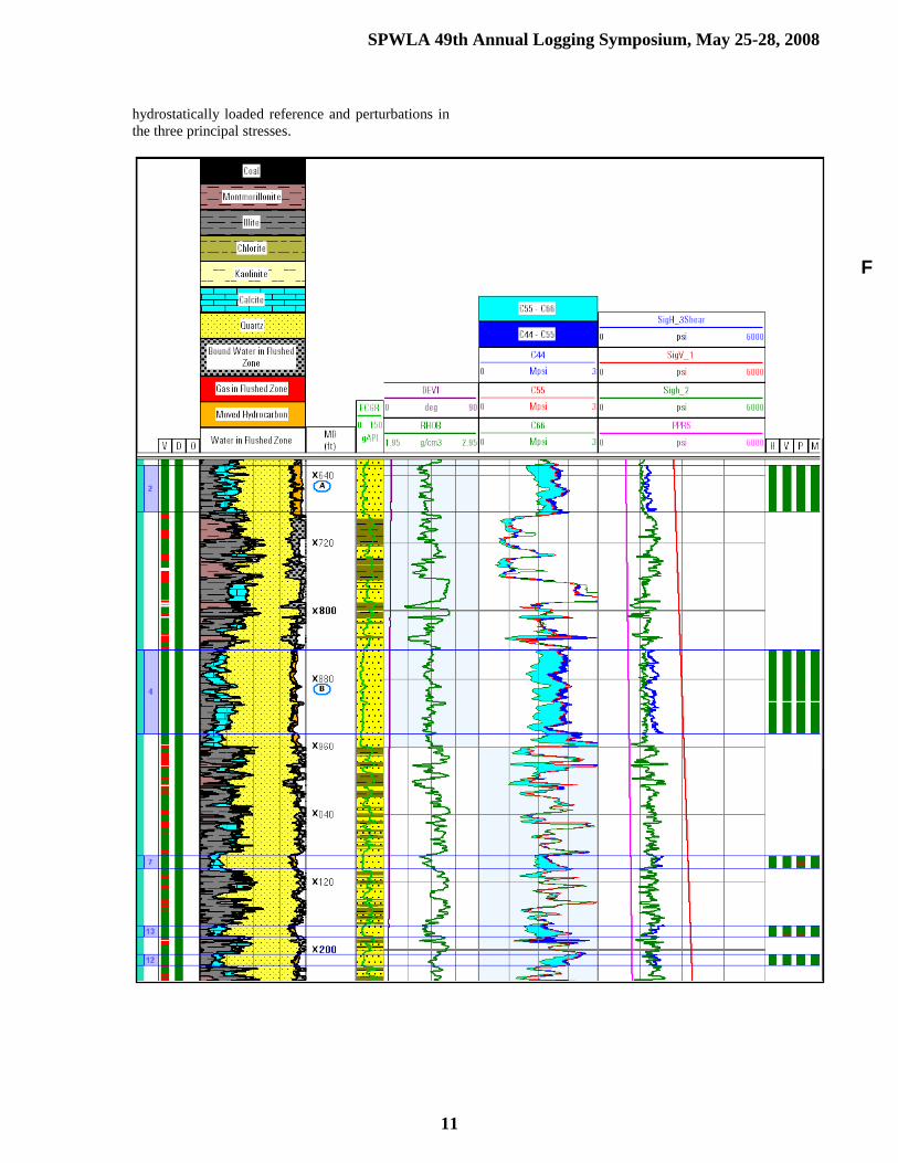
Figure 4. Composite logs of elemental analysis (ELAN), gamma ray, borehole deviation, formation bulk density, the

far-field shear moduli, the overburden, maximum and minimum horizontal stresses, and pore pressure.

Figure 5a. Measured borehole dispersions together with theoretical dispersions for an equivalent isotropic and

radially homogeneous formation at depth A (marked in Figure 4). The red and blue markers denote the fast and slow

dipole dispersions, respectively. The cyan markers represent the Stoneley dispersion.

Figure 5b. The notation is the same as in Figure 5a. Results are for depth B (marked in Figure 4) in a sand reservoir.


12

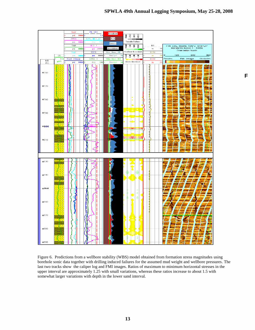
Figure 6. Predictions from a wellbore stability (WBS) model obtained from formation stress magnitudes using

borehole sonic data together with drilling induced failures for the assumed mud weight and wellbore pressures. The

last two tracks show the caliper log and FMI images. Ratios of maximum to minimum horizontal stresses in the

upper interval are approximately 1.25 with small variations, whereas these ratios increase to about 1.5 with

somewhat larger variations with depth in the lower sand interval.

F


13

Figure 7. Composite logs of gamma ray, wellbore deviation, calipers, formation bulk density, compressional and

shear slownesses, overburden stress, pore pressure, and estimated horizontal stress gradients in various lithology

intervals using the VDG technique


14

Figure 8a. Measured borehole dispersions at depths C1 and C2 (marked in Figure 7) in a clay-dominated interval.

The orange and green markers denote the best curve fits to measured dipole dispersions at these two depths. The

cyan and brown markers represent the Stoneley dispersions at the two depths.

Figure 8b. The notation is the same as in Figure 8a. Results are for depths D1 and D2 (marked in Figure 7) ft in a

sand interval.

F


15

Figure 9. Predictions from a WBS model obtained from formation stress magnitudes from the VDG algorithm using

borehole sonic data show improved agreement with observed drilling-induced failures in the bottom interval than

was the case with stress magnitudes obtained using an existing estimation technique. The last two tracks show the

caliper logs delineating breakout intervals.


16

Documents

Estimation Of Formation Stresses Using Borehole Sonic …€¦ · ESTIMATION OF FORMATION STRESSES USING BOREHOLE SONIC DATA Bikash K. Sinha, Jing Wang, Saad Kisra, Ji Li, Vivian