Estimation of discontinuity spacing and trace length using scanline surveys

Int. J. Rock Mech. Min. Sci. & Geomech. Abstr. Vol. 18, pp. 183 to 197, 1981 0148-9062/81/030183-15502.00/0 Printed in Great Britain Pergamon Press Ltd

Estimation of Discontinuity Spacing and Trace Length Using Scanline Surveys S. D. PRIEST* J. A. HUDSON,"

Knowledge of the spacing and size of discontinuities in a rock mass is of considerable importance for the prediction of rock behaviour. The characteristics of discontinuities can be estimated using scanline surveys but the precision of the estimates must be obtained and the bias caused by linear sampling must be eliminated before they can validly be used. Initially, an expression is presented which gives the degree of confidence that can be assigned to the measured mean discontinuity spacing. A reduced form of this expression is obtained for cases where the discontinuity spacings follow the negative exponential distribution. The precision of discontinuity frequency and RQD estimates is also explained. The distribution of trace lengths produced by the intersection of planar discontinuities with a planar rock face is used to determine the distribution of trace lengths, the distribution of semi- trace lengths and the distribution of censored semi-trace lengths intersected by a randomly located scanline. Comparison of the actual and sampled distributions demonstrates the bias introduced by scanline sampling of trace lengths. Relations between the distributions can be used to produce analytical or graphical methods of estimating mean trace length from censored measurements at exposures of limited extent.

INTRODUCTION

In order to characterize rock mass geometry for engineering purposes, discontinuity surveys usually include measurements of discontinuity spacing and trace length. It is critically important to estimate these parameters with the necessary accuracy and precision by obtaining a representative and sufficient sample of spacings and trace lengths from the rock mass domain in question. Also the sample values should either be unbiased or the bias should be understood and eliminated. The scanline survey, which involves sampling and measuring only those discontinuities that intersect a line set on the surface of the rock mass, provides a very convenient means of obtaining such a sample but, in the case of trace lengths, the raw data will be biased.

The purpose of this paper is

(a) to show how the reliability of mean discontinuity spacing values obtained from scanline surveys can be assessed and

* Department of Mineral Resources Engineering, Imperial College of Science and Technology, South Kensington, London SW7 2BP, U.K.

t Geotechnics Division, Building Research Station, Garston, Wat- ford, Hefts WD2 7JR, U.K.

(b) to demonstrate why scanlines provide a biased sample of discontinuity trace lengths and to explain how this bias can be overcome.

The terms used in this paper are defined as follows and summarized in Table 1:

Discontinuity: A general term for any mechanical break that has zero or relatively low tensile strength in a rock mass. The term includes such features as joints, fractures, fissures, weak bedding planes and faults [1].

Discontinuity spacing, x: The distance between an adjacent pair of discontinuities measured along a straight line of a given orientation within, or on the surface of, a rock mass. In general, the value varies with both scanline orientation and location but, if the discontinuities were parallel, the value would only depend on scanline orientation. These and other aspects of discontinuity spacing measurements have been discussed by Hudson & Priest [2-1.

Mean discontinuity spacing, Y: The mean value of spacings computed as

= ~ xdn i=1

where xi is the ith discontinuity spacing measurement

183

184 S .D. Priest and J. A. Hudson

along a scanline of length X yielding n values:~. For practical and theoretical reasons it is desirable to take the distance from the start of the scanline to the first discontinuity and add it to the distance between the nth discontinuity and the end of the scanline, in order to generate the nth spacing value.

Mean discontinuity frequency: The mean number of discontinuities encountered per unit length along a scanline and hence the reciprocal of mean discontinuity spacing. The mean discontinuity frequency is a measure of the 'degree of brokenness' along a line in a given direction through a rock mass and applies for any discontinuity geometry. For a large sample, 1/Y = n/X -~ 2 = mean discontinuity frequency for the population.

Discontinuity trace length, l: The measurable length of the linear trace produced by the intersection of a planar discontinuity with a planar rock face. The end of a trace will occur either at another discontinuity or within the rock material [1]. The end of a trace may not, however, be visible at a given face due to excava- tion, erosion or the presence of vegetation or scree covering.

Mean discontinuity trace length, 7: The mean value of trace lengths computed as

-l = ~.. lJn i = 1

where li is the ith discontinuity trace length sampled in some specified way at a given rock face that yields a total of n such trace lengths.

Mean trace termination frequency: This is defined as the reciprocal of mean discontinuity trace length and is therefore analogous to mean discontinuity frequency. For a large sample, 1/7 ~ # = mean trace termination frequency for the population.

Semi-trace length, l: That portion of the trace length between the scanline intersection point and the end of the trace. The sum of the two semi-trace lengths, one in either direction from the scanline, for a particular discontinuity, is the total trace length.

Censored semi-trace length, l: The length of the trace from the scanline to one end of the trace or a fixed distance, c, whichever is least. The letter I has been used to denote the trace length, the semi-trace length and the censored semi-trace length. The functional letter corresponding to the probability density distribution, e.g. g(l) for the intersected complete trace lengths, distinguishes the type of trace length in question. A list of these distributions is given in the introduction to the section on estimating discontinuity trace length.

Rock mass domain: This is a portion of a given rock mass in which discontinuity characteristics, in particular mean spacing and mean trace length, are con-

Lower case italic letters have been used throughout for theoretical and sampled values of spacing and trace length.

TABLE 1. SUMMARY OF TERMS USED

Spacing Trace length

General value x / ith value xl /~ Total number in a sample n n

Summed length of values X = ~ xi L = ~ l, i : l i 1

Mean value x = X/n I = L/n Mean population frequency estimate* ,;~ = 1/~ p = Ill

* The population frequency parameters ). and p are adopted in this paper to facilitate the theoretical analysis and permit comparisons with previous work.

stant; in other words, a part of a rock mass that is statistically homogeneous. Variation of the measured values of mean spacing and trace length across a rock mass domain is, therefore, only a function of the sampling method since, by definition, there is no change in the discontinuity characteristics. The calculations in this paper are for rock mass domains but extension of the ideas to inhomogeneous rock masses is possible by using the geostatistical method [3].

The first part of this paper concerns the precision of mean discontinuity spacing, discontinuity frequency and Rock Quality Designation estimates from measurements taken along a scanline set up on a planar rock face. Some explanation of sampling theory is included at the outset to provide the necessary framework for subsequent analysis. The second part of the paper, which covers discontinuity trace length, relates to ideas originally presented by Cruden [4] and extends these to account for the fact that a scanline will tend to intersect, and therefore sample, the longer trace lengths in preference to shorter ones on a given rock face. The resulting sampling bias depends upon the distribution of trace lengths in the rock mass and can, in certain circumstances, be quite significant. This, and other theoretical and practical aspects of trace length measurements are discussed.

P R E C I S I O N O F T H E MEAN D I S C O N T I N U I T Y SPACING, D I S C O N T I N U I T Y

F R E Q U E N C Y A N D R Q D ESTIMATES

The mean discontinuity spacing estimate

During a scanline survey, one survey group might measure, say, 100 discontinuities to compute mean discontinuity spacing. A second survey group might spend more time and measure 300 discontinuities. The value of mean discontinuity spacing estimated by the second group will certainly be more reliable than that estimated by the first. Lacking further information, it is difficult to decide whether the increased effort of the second group can be justified by the increased reliability of their result.

Obtaining a balance between the effort expended in obtaining a sample and the reliability of the result

Estimation of Discontinuity Spacing 185

requires some method of calculating the precision. This can be achieved using a standard statistical method [5, 6] based on the central limit theorem which states that the means of random samples of size n taken from a population that follows any distribution, with a mean 1/2, and standard deviation a, will tend to be normally distributed with a mean 1/2 and standard deviation tr/x/n. The term tr/x/n is called the standard error of the mean. The distribution of means is only approximately normal for values of n < 30, but becomes closely normal for larger values of n.

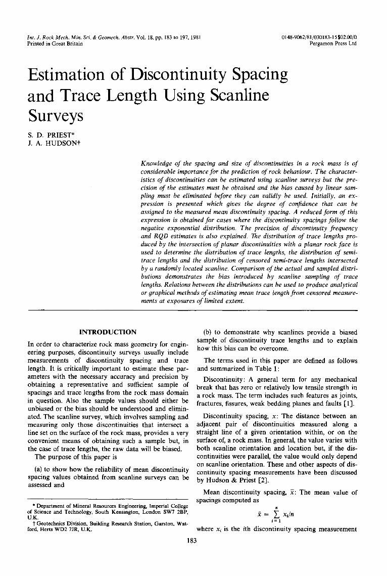
In the context of discontinuity measurements, the population can be regarded as consisting of all possible measurements of discontinuity spacing in a given direction throughout the rock mass domain. If scanline sampling of n discontinuities were carried out in the same direction at several different locations within the domain it would, in theory, be possible to plot the frequency distribution of the various resulting mean values, £. According to the central limit theorem, such a distribution will, for large values of n, tend to have the characteristic bell shape of the normal distribution, irrespective of the distribution of discontinuity spacings in the population (Fig. la).

Given the well-defined properties of the normal distribution, it is known that a proportion ~(z) of the many different scanlines in the same direction will yield a mean value within ++_za/x/n of the population mean (Fig. lb) where z is the standard normal variable associated with a certain confidence level. Selected values of z and q~(z) are given in Table 2. More comprehensive tabulations can be found in most statistical textbooks.

For discontinuity spacing values measured along a scanline, therefore, the mean value has a ~(z) probability (i.e. 100 ~(z) Vo confidence) of lying within the

! I

ca)

Sample mean, x

Frequency

Population meon,~.~_ z o

(b) . . . .

qb ( z ) - shoded anm / to~l oreo

~ the curve

I

Fig. 1. Frequency distribution of the sample mean.

TABLE 2. VALUES OF (ib(2) FOR

THE NORMAL DISTRIBUTION

z ~(z)

0.675 0.50 0.842 0.60 1.036 0.70 1.282 0.80 1.645 0.90 1.960 0.95 2.576 0.99

range ++_za/x/n of the population mean. This gives a direct measure of the reliability of the result obtained using this scanline. Although a is unknown because it is the population rather than sample standard deviation, for most practical purposes a may be taken as equal to the standard deviation of the sample. As an example, assume that the standard deviation of 80 discontinuity spacing values measured along a 14m scanline is 0.160m. The mean discontinuity spacing is 0.175m with a/x/n = 0.160/x/80 = 0.018m. Selecting a 953/0 confidence band, q~(z) = 0.95 giving z = 1.960, it can be concluded that there is 95Yo confidence that the mean value 0.175 m lies within _+0.035 m of the population mean. In other words there is 95~ confidence that the population mean lies somewhere in the range 0.140q).210m, regardless of the discontinuity spacing distribution.

An interesting and useful reduction of the formula occurs if the discontinuity spacing values follow a negative exponential distribution; there is considerable justi- fication for assuming that many rock masses exhibit this form of spacing distribution [7, 8, 9]. The frequency, f (x), of a given discontinuity spacing value x is then given by the following probability density distribution:

f ( x ) = ).e -~x (1)

The significance of this distribution in the present context is that the mean and standard deviation of the population are equal or, for a large sample from the population, have the same expected value.

For a sample of size n, the bandwidth of 100 q)(z)~ confidence is now obtained by substituting ~ for tr in the previous expressions giving £ _+ (z:i)/x/n. Alterna- tively, this bandwidth can be written as

where • is the allowable proportionate error.

Hence

or

= z / , / , ,

n = (z/E) 2 (2)

Equation (2) can be used to compute the sample size required to achieve a given error bandwidth simply by substituting the appropriate values of z and E corresponding to the required confidence level and the

186 S.D. Priest and J. A. Hudson

desired error bandwidth. Conversely, the expression can be used to establish the error limits given by a certain sample size.

For example, if the mean spacing is required within an error bandwidth of + 20% at the 80% confidence level, c = 0.2, z = 1.282 and

(,28:y n /> 0.2 / = 41.

If the mean spacing is required within + 10% at the 90% confidence level, E = 0.1, z -- 1.645 and

(1.645~: n ~ > 0_1 # = 2 7 1 .

These results show that sample sizes of several hundreds are required to give reasonably reliable estimates.

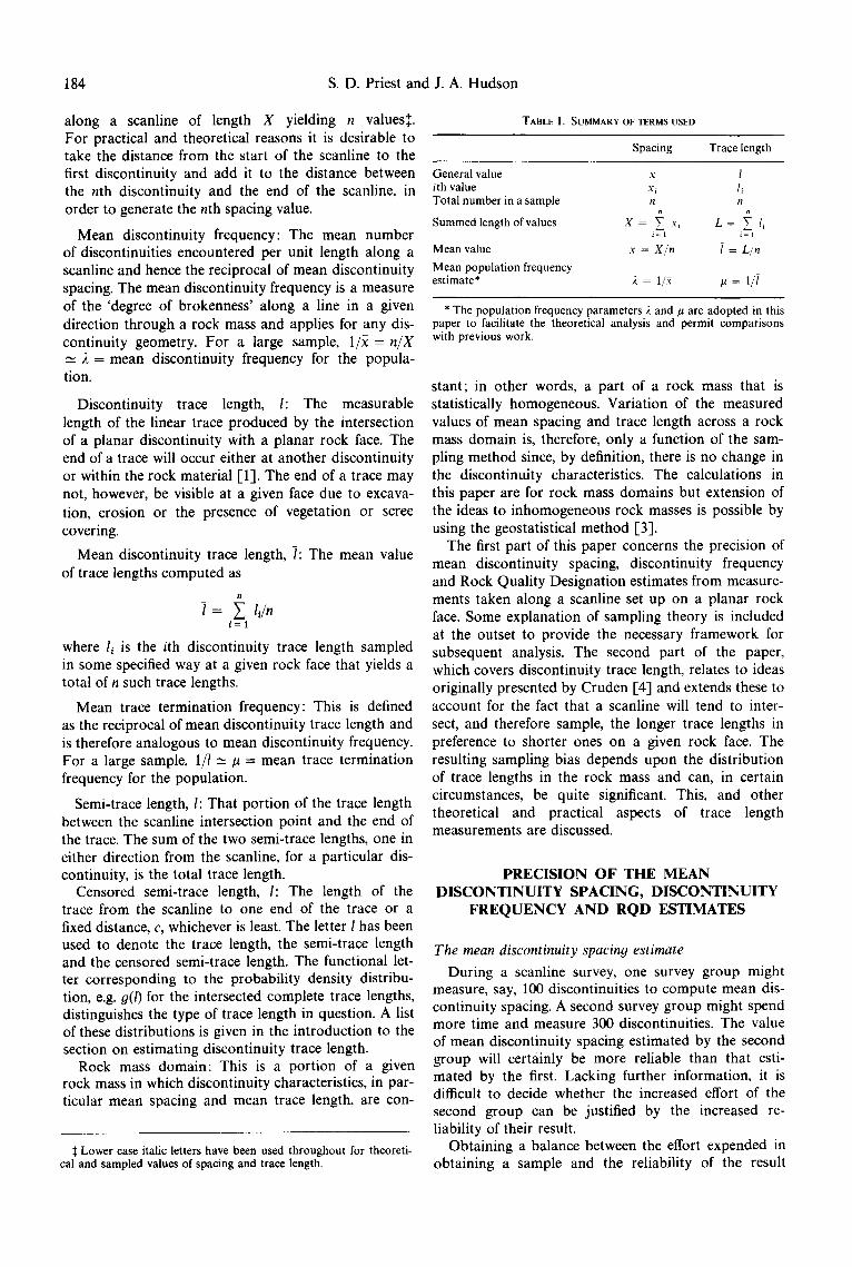
A graph illustrating the number of spacing values required versus the error band for various confidence levels is shown in Fig. 2. The previous examples and this graph demonstrate that the required sample size increases very rapidly as the allowable error is reduced.

Computation of the error band defined by a given sample size can be illustrated using the previous example where 80 discontinuities measured along a 14 m scanline gave ~ = 0.175m. This time, ignoring the computed value of a, and taking the 95,°<, confidence level z = 1.960, gives

1.960 e - - 0.219

\ 8 0

which defines a 95% confidence bandwidth of 0.137- 0.213m.

The discontinuity frequency estimate

If the reliability of the discontinuity frequency is required rather than the mean spacing value for a given sample size, the reciprocal of the values defining the spacing bandwidth are taken. In the last example above, the 95% confidence frequency bandwidth is 7.32-4.69 per m, a result that is not symmetrical about the mean of 5.71 per m.

The RQD estimate

The values of mean discontinuity spacing and frequency can be measured by scanline surveys and their reliability can be estimated by the technique described above. The values provide an indication of rock quality themselves but, through the distribution of spacing values, a relation can be established with the Rock Quality Designation. Thus the precision of the 2 estimate has direct implications for the precision of the theoretical RQD which is briefly explained below.

The theoretical RQD, being analogous to RQD measured in the usual way from borehole core, is found by integrating all spacing values above 0.1 m and expressing the resultant value as a proportion of the summed length of all spacing values [7]. Whilst the theoretical RQD can be found from any distribution ot spacing values, it is assumed here that the discontinuity spacings along the scanline or borehole follow the negative exponential distribution (equation 1).

The percentage length of the scanline or borehole consisting of spacing values greater than a given value, t, gives the theoretical RQD, RQD*, as

RQD* = 100 e -'~ (t2 + 1) (3)

35° I 300 1 5 0 6 0 7 0 8 0 9 0 9 5 9 9 % confidence

: 2 5 0

E

t~ 200 .c

"~ 150

i I00

~ 50 m - -

I [ I 0.05 OJO 0.15 0 2 0 0 .25

Proportionate error in mean discontinuity spacing, E

I

0.50

Fig. 2. Sample number vs precision of the mean discontinuity spacing estimate for a negative exponential distribution of spacings.


Since this formula is derived simply by integrating all spacing values above the threshold value t in the spacing distribution, expressions for theoretical RQD can be found in a similar manner for other forms of the spacing distribution f(x). If t is set equal to 0.1 m, then the value of RQD* is directly equivalent to the conven- tional RQD. Wallis & King [9-] have found that RQD values computed using equation (3) agree well with measured values for a Pre-Cambrian granite in Mani- toba.

Priest & Hudson [7-] have shown that a good linear approximation to equation (3) for t = 0.1 m is given by the tangent at the inflection point. This tangent is given as

RQD* = 110.4 - 3.68). (4)

and provides a reasonable approximation in the range 6 < 2 < 16 per m. It is interesting to note that the International Society for Rock Mechanics [1] has pro- posed the following approximate empirical relation between RQD and the volumetric joint count Jv

RQD = 115 - 3.3 Jv for Jv >/4.5

RQD = 100 for J~ < 4.5

where Jo is defined as the sum of the number of joints per m for each joint set present.

The precision of the theoretical RQD estimate can be determined in either case by calculating the upper and lower brackets for 2 from equation (2) and substituting the values in either of the RQD formulae to give the lower and upper brackets of RQD. The value of RQD* and/or the original value of 2 as estimated by 1/~ can be used as an input to rock classification schemes [10, 11] which, by combining these and other parameters relating to the rock mass and rock material properties, will give some indication of the likely engineering performance of the rock mass. Whether the value of mean discontinuity spacing or frequency is used directly or processed in some way, it is clearly desirable that the precision of the value should be known.

ESTIMATING DISCONTINUITY TRACE LENGTH

The extent of a given discontinuity, or set of discontinuities, can play a major role in controlling the behaviour of a rock mass. It may be desirable, therefore, during a scanline survey to record information concerning the extent of discontinuities intersected. At a planar, or nearly planar, face the simplest measure of discontinuity extent is the length of the trace produced by the intersection of a given discontinuity with the rock face. Theoretical studies of the distribution of trace lengths generated by the intersection of randomly located planar discontinuities with a planar rock face have been discussed elsewhere [12, 13] and Cruden [4] has explained in detail the techniques and problems associated with trace length measurements. The analysis in this paper is concerned with estimation of trace length

distributions rather than the reason why a particular distribution might exist.

The estimation problem discussed in the previous section was one of precision; it was assumed that the spacing values had been obtained without introducing any bias so that the mean of the scanline measurements would tend to the population mean. However, values of trace length obtained using the same scanline survey technique contain an inherent and significant bias which must be accounted for during the data reduction stage. The problem of estimating trace length, therefore, is one of both accuracy and precision.

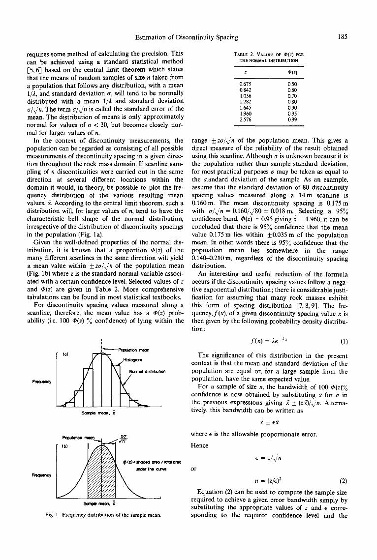
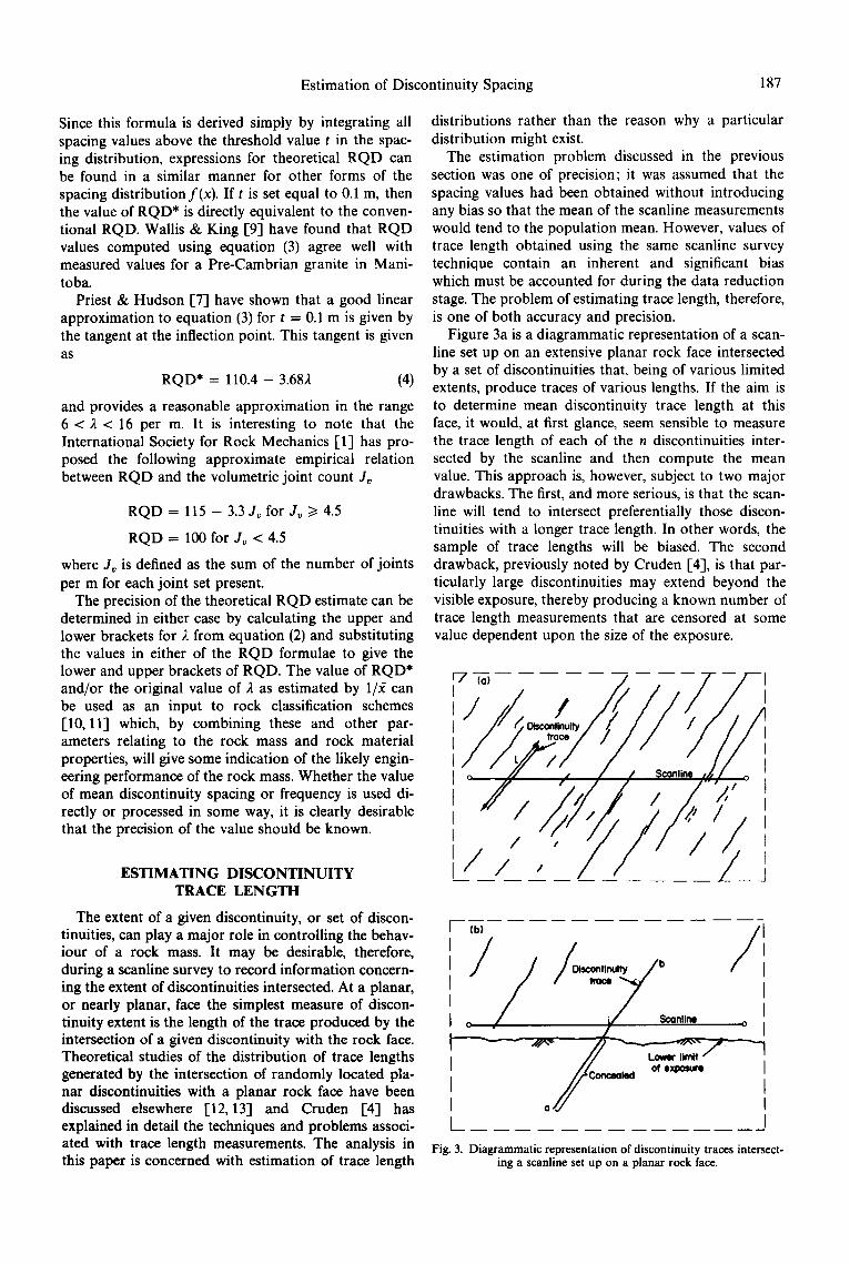
Figure 3a is a diagrammatic representation of a scanline set up on an extensive planar rock face intersected by a set of discontinuities that, being of various limited extents, produce traces of various lengths. If the aim is to determine mean discontinuity trace length at this face, it would, at first glance, seem sensible to measure the trace length of each of the n discontinuities intersected by the scanline and then compute the mean value. This approach is, however, subject to two major drawbacks. The first, and more serious, is that the scanline will tend to intersect preferentially those discontinuities with a longer trace length. In other words, the sample of trace lengths will be biased. The second drawback, previously noted by Cruden [4], is that particularly large discontinuities may extend beyond the visible exposure, thereby producing a known number of trace length measurements that are censored at some value dependent upon the size of the exposure.

7 Io)

/ / Scanline 1~

/ / /

/ /

o f ~ / " # X I I'/I " i

",'?//"> S

Y

I I I I I

I

(hi / I

I ~ / Sconllne o I J

Concealed of exposure

, ( / I I

Fig. 3. Diagrammatic representation of discontinuity traces intersecting a scanline set up on a planar rock face.

188 S. D. Priest and J. A. Hudson

TABLE 3. TRACE LENGTH DISTRIBUTIONS

Probability density Population Estimated distribution mean mean

Trace length Intersected trace length Semi-trace length Censored semi-trace length

f (t) 1/~ -1

h(I) 1 /~ h lh i(I) 1/12i -1 i

Cruden [4] also drew attention to the problem of particularly small discontinuities, so small in fact that they are difficult, if not impossible, to measure. This produces an unknown number of trace length measurements that are truncated at some small value dependent upon the measurement procedure. In the authors' ex- perience, it is certainly feasible to observe and measure trace lengths as low as 10mm both in the field and from photographs. Truncation at this level will therefore have only a small effect on the data, particularly if the mean trace length is in the order of metres.

The following discussion deals with the problem of preferential intersection of the longer trace lengths, measuring trace lengths on one side of the scanline only and the problems of trace length censoring at limited exposure areas. The distributions discussed are listed in Table 3.

Trace length sampling bias

The probability density distribution of trace lengths over the entire rock face is denoted by f ( l ) and the cumulative probability distribution by F(l). At this stage no assumptions are made concerning the nature off(I).

If the scanline is located randomly with respect to a set of parallel discontinuity traces then the probability of the scanline intersecting a given trace is directly proportional to the length of that trace. Therefore the probability, p(1), that the scanline intersects a trace with a length in the range 1 to l + d l is given by

p(l) = k l f (l)dl (5)

where k is a constant. The probability density distribution, g(l), of trace

lengths intersected by the scanline is therefore given by

g(l) = k l f (l) (1 > O)

given that g(l) is a probability density distribution, then

or

but

ff ' g(l) dl = 1

k I f ( l ) dl = 1

f f 1 I f ( l ) dl = - It

therefore

and

k = l~

g(l) = Mlf ( l ) . (6)

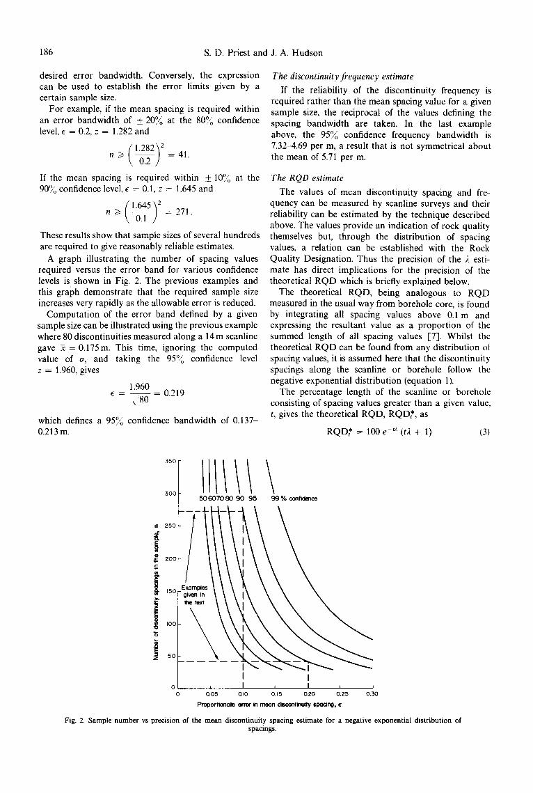
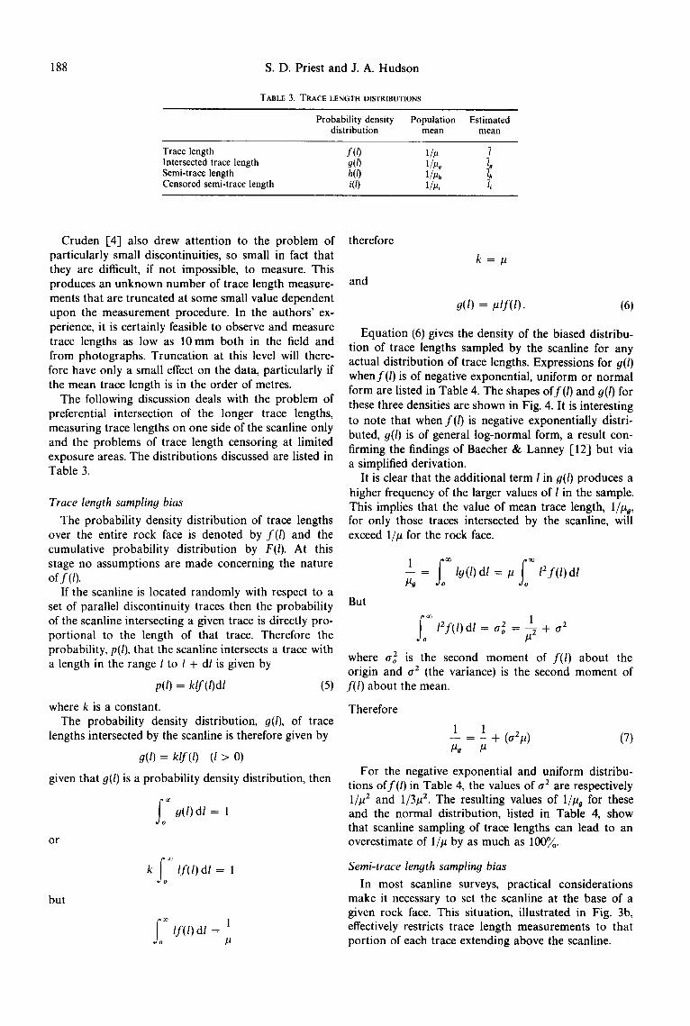
Equation (6) gives the density of the biased distribution of trace lengths sampled by the scanline for any actual distribution of trace lengths. Expressions for g(l) when f(/) is of negative exponential, uniform or normal form are listed in Table 4. The shapes off(I) and g(l) for these three densities are shown in Fig. 4. It is interesting to note that when f (1) is negative exponentially d~stri- buted, g(l) is of general log-normal form, a result con- firming the findings of Baecher & Lanney [12] but via a simplified derivation.

It is clear that the additional term I in 9(l) produces a higher frequency of the larger values of l in the sample. This implies that the value of mean trace length, 1/#g, for only those traces intersected by the scanline, will exceed 1/p for the rock face.

But

If) ;) - = l g ( l ) d l = u 1 2 f ( l ) d t Pg

~o ~ 2 ~--- ] 12f( l )d l = ao ~ + a 2

2 is the second moment of f ( l ) about the where a o origin and a 2 (the variance) is the second moment of f ( I ) about the mean.

Therefore

1 1 - + (a2M) (7)

For the negative exponential and uniform distributions off(l) in Table 4, the values of a 2 are respectively 1/p 2 and 1/3p 2. The resulting values of 1/#g for these and the normal distribution, listed in Table 4, show that scanline sampling of trace lengths can lead to an overestimate of 1/p by as much as 100~.

Semi- t race length sampling bias

In most scanline surveys, practical considerations make it necessary to set the scanline at the base of a given rock face. This situation, illustrated in Fig. 3b, effectively restricts trace length measurements to that portion of each trace extending above the scanline.


1.0

Pmlxlbllity density

0.5

o o

• Negative exponential p. • I ~ t trace k ~

glLlintersected trace lengths

1.0 2.0 3.0 Truce length

i .o r Uniform p. , I

/ Probability l . I

clonsily ] f(I,) i ~ ~" , ' / ,.,r. I

o 0 l.O

T r a c e length

1"1 f

2.0

1.5 Normal # , I a - I / 3

obob,,; o 0'L'

o ,

0 1.0 2.0 3.0

Trace length

Fig. 4. Probability density distributions of actual trace lengths, f(/), and intersected trace lengths, g(l), where f( / ) is of negative exponential, uniform and normal form.

In Fig. 3b, the full length of a randomly intersected discontinuity trace, ab has a probability density g(l) and a cumulative probability distribution G(/). Because the scanline is located near to the edge of the exposure, it will usually only be possible to measure the semi-trace length, ib, of a given trace whose end b is visible. It is therefore necessary to consider the probability density distribution h(l) and cumulative probability distribution H(l) of the semi-trace lengths intersected by the scanline.

The distribution h(l) is derived as follows using a substitute variable m representing complete trace length.

1. The intersected complete trace length, a b = m, has a probability density distribution g(m) as obtained in the previous section. The probability that the complete trace length lies in the range m to m + dm is therefore g(m)dm.

2. Since the intersection point i is randomly located along ab (Fig. 3b), the semi-trace length measured from i to b, is uniformly distributed in the range 0 to m with

a probability density distribution of 1/m. Hence the probability that the semi-trace length lies in the range l to l + dl is (1/m)dl.

3. The probability, p(m, l), that the complete trace length lies in the range m to m + d m and that the semi- trace length lies in the range l to l + dl is given by

p(m, l) = g(m)dm (l/m) dl (8)

4. To obtain the probability, p(l), that the semi-trace length lies in the range l to l + dl for any total trace length, it is necessary to sum all p(m, l) for all possible values of m. Since p(m, l) is zero for any values of m that are less than l, it is necessary to integrate equation (8) with respect to m between I and infinity.

p(l) = (l/m) dl o(m) am = h(l) dl

o r

~l °° h(l) = (1/m)g(m) dm

190 S . D . Priest and J. A. Hudson

io

~ l i t y density

o5

. Negative exponential F= I

j f(I,)Actual trace lengths ~ " " " ~ e -- h(b)semJ-trace lengths

I

0 2.0 3.0

~0

0 0

Probability der--ity

05

I0

Trace length or semi-trace length

~ Uniform /~ - I

" - ........_ h ( I, )

"~,, f( I ,)

l " I I/Fh ] I /F ~ .~

I0 2 0

Trace length or semi- ~roce length

15

I0 Probability

densay

0.5

Normol / z , l c r , l l 3

h(I,)

N \ \

I

0 I0 20 3 0

Troce length or semi-trace length

Fig. 5. Probability density distributions of actual trace lengths, f( l) , and semi-trace lengths, h(l), where f ( l ) is of negative exponential, uniform and normal form.

But

Hence

o r

g(m) = #mf(m)

~ ot~

h(l) = la f(m) dm

h(1) = #(1 - F(l)) (9)

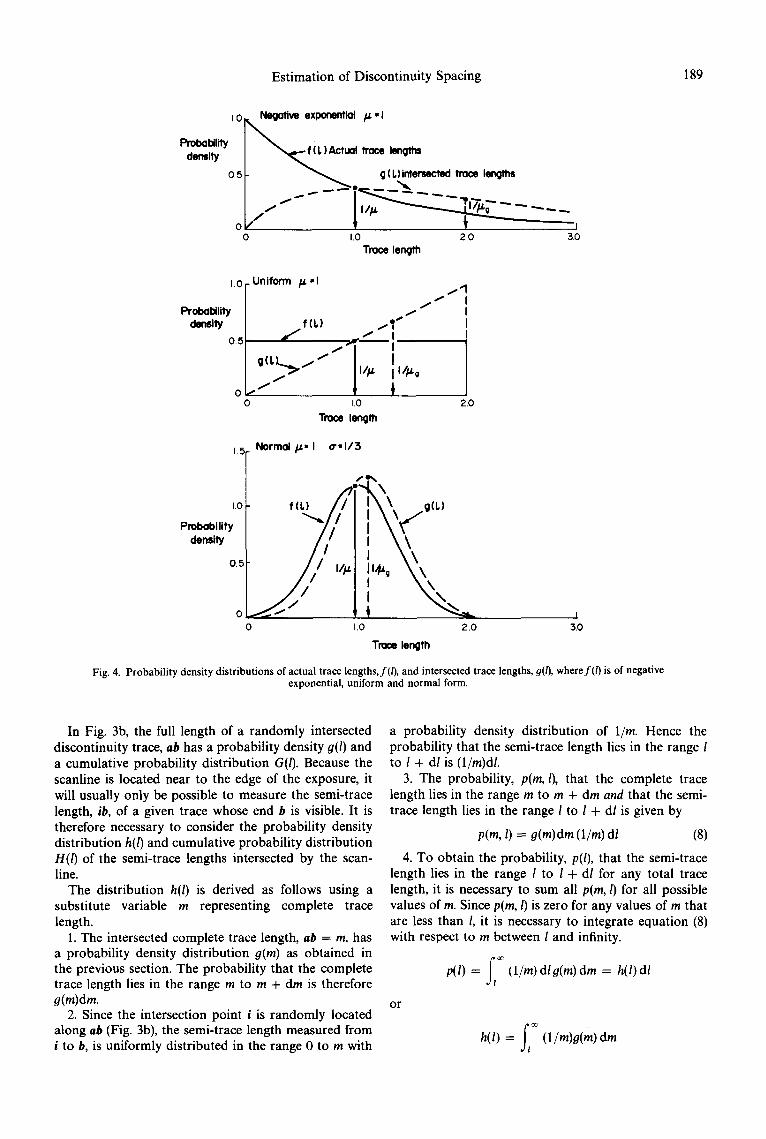
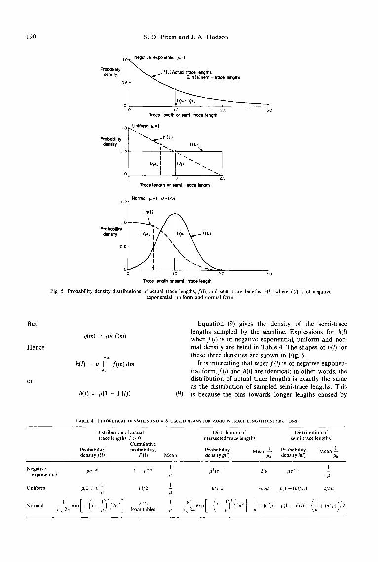
Equation (9) gives the density of the semi-trace lengths sampled by the scanline. Expressions for h(l) when f ( l ) is of negative exponential, uniform and normal density are listed in Table 4. The shapes of h(l) for these three densities are shown in Fig. 5.

It is interesting that when f( /) is of negative exponential form, f ( l ) and h(I) are identical; in other words, the distribution of actual trace lengths is exactly the same as the distribution of sampled semi-trace lengths. This is because the bias towards longer lengths caused by

TABLE 4, THEORETICAL DENSITIES AND ASSOCIATED MEANS FOR VARIOUS TRACE LENGTH DISTRIBUTIONS

Distribution of actual Distribution of trace lengths, I > 0 intersected trace lengths

Cumulative Probability probability, Probability Mean l density f(/) F(I) Mean density g(l) #o

Distribution of semi-trace lengths

Probability Mean 1 density h(l) I~h

l Negative #e ,,i 1 - e -m -- #21e-'a 2/# exponential #

2 I Uniform #/2, I <~ - #1/2 - #2 I/2 4/3#

# #

1 _ _ _ _ + (a~#) Normal - 1 - F(l) 1 #1 - I - | a \ from tables # a \ 2n ~ '/ #

#e-J d

#(1 - ( ~ U 2 ) )

#(1 - F(h)

2/3#


V--

I

L

- oT/

.J

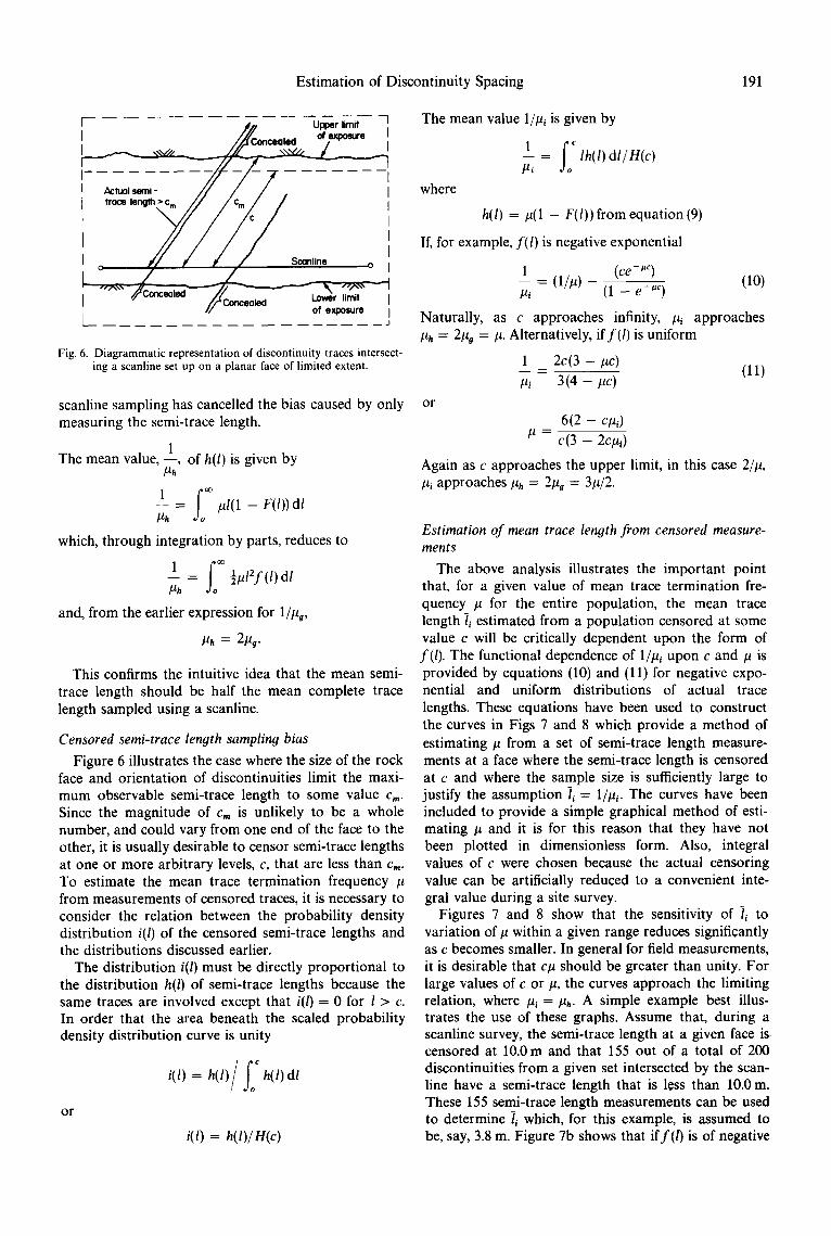
Fig. 6. Diagrammatic representation of discontinuity traces intersecting a scanline set up on a planar face of limited extent.

scanline sampling has cancelled the bias caused by only measuring the semi-trace length.

1 The mean value, - - , of h(l) is given by

Ph

ff - - = # 1 ( 1 - F q ) ) d t Ph

which, through integration by parts, reduces to

1 fo~ - - = ½ # 1 2 f ( l ) dl #,

and, from the earlier expression for 1/#g,

#h = 2#g.

This confirms the intuitive idea that the mean semi- trace length should be half the mean complete trace length sampled using a scanline.

Censored semi-trace length sampling bias

Figure 6 illustrates the case where the size of the rock face and orientation of discontinuities limit the maximum observable semi-trace length to some value c~. Since the magnitude of cm is unlikely to be a whole number, and could vary from one end of the face to the other, it is usually desirable to censor semi-trace lengths at one or more arbitrary levels, c, that are less than cm. To estimate the mean trace termination frequency p from measurements of censored traces, it is necessary to consider the relation between the probability density distribution i(l) of the censored semi-trace lengths and the distributions discussed earlier.

The distribution i(l) must be directly proportional to the distribution h(l) of semi-trace lengths because the same traces are involved except that i(l) = 0 for l > c. In order that the area beneath the scaled probability density distribution curve is unity

/ fo c i(I) = h(l) h(l)dl

o r

i(I) = h(l)/H(c)

The mean value 1/#, is given by

1 f f - - = lh(l) dl /H(c) #i

where

h(l) = #(1 - F(I)) from equation (9)

If, for example, f ( l ) is negative exponential

1 (ce -uc) - - = (1 /#) (10) Pi (1 -- e -~c)

Naturally, as c approaches infinity, #~ approaches #h = 2#g ---- #. Alternatively, if f ( / ) is uniform

1 2c(3 - pc) - (11)

#~ 3(4 - pc)

o r

6(2 - cpi) # - c(3 - 2c#i)

Again as c approaches the upper limit, in this case 2/#, #~ approaches #h = 2#g = 3#/2.

Estimation of mean trace length from censored measurements

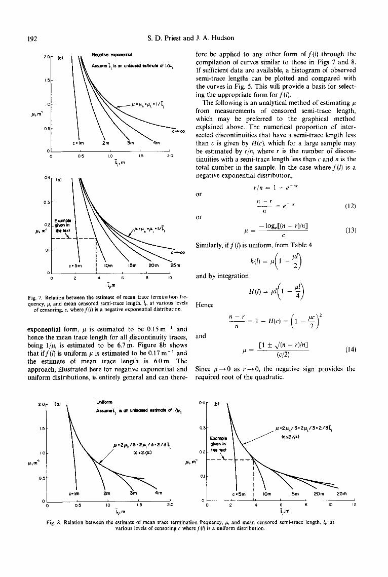
The above analysis illustrates the important point that, for a given value of mean trace termination frequency # for the entire population, the mean trace length li estimated from a population censored at some value c will be critically dependent upon the form of f(1). The functional dependence of 1/#i upon c and # is provided by equations (10) and (1 l) for negative exponential and uniform distributions of actual trace lengths. These equations have been used to construct the curves in Figs 7 and 8 which provide a method of estimating # from a set of semi-trace length measurements at a face where the semi-trace length is censored at c and where the sample size is sufficiently large to justify the assumption li = 1/pi. The curves have been included to provide a simple graphical method of estimating # and it is for this reason that they have not been plotted in dimensionless form. Also, integral values of c were chosen because the actual censoring value can be artificially reduced to a convenient integral value during a site survey.

Figures 7 and 8 show that the sensitivity of 7~ to variation of # within a given range reduces significantly as c becomes smaller. In general for field measurements, it is desirable that c# should be greater than unity. For large values of c or #, the curves approach the limiting relation, where #i = #h. A simple example best illustrates the use of these graphs. Assume that, during a scanline survey, the semi-trace length at a given face is. censored at 10.0 m and that 155 out of a total of 200 discontinuities from a given set intersected by the scanline have a semi-trace length that is less than 10.0 m. These 155 semi-trace length measurements can be used to determine li which, for this example, is assumed to be, say, 3.8 m. Figure 7b shows that if f ( / ) is of negative

192 S . D . Priest and J. A. H u d s o n

I 0

/.~,m "1

2.0 (o)

15

0 0

0 5

NeQative exponential

is on unbiased estimate of I//J, I

c _ o

I I I I 0 5 1.0 1.5 2 0

I,? m

041 (b)

0 3 I

Exomple 0 2 . given in

# , m "1 ffw! texV

OI

0

1

clSm

2

I IOm 15m 20m 25m I I 1 I I

4 6 8 I0

iem

Fig. 7. Relation between the estimate of mean trace termination frequency, #, and mean censored semi-trace length, 1i, at various levels

of censoring, c, where f ( / ) is a negative exponential distribution.

exponential form, /~ is estimated to be 0.15 m-1 and hence the mean trace length for all discontinuity traces, being l/g, is estimated to be 6.7 m. Figure 8b shows that if f( /) is uniform/~ is estimated to be 0.17 m- ' and the estimate of mean trace length is 6.0m. The approach, illustrated here for negative exponential and uniform distributions, is entirely general and can there-

fore be applied to any other form of f ( l ) through the compilation of curves similar to those in Figs 7 and 8. If sufficient data are available, a histogram of observed semi-trace lengths can be plotted and compared with the curves in Fig. 5. This will provide a basis for selecting the appropriate form for f(l).

The following is an analytical method of estimating/~ from measurements of censored semi-trace length, which may be preferred to the graphical method explained above. The numerical proportion of intersected discontinuities that have a semi-trace length less than c is given by H(c) , which for a large sample may be estimated by r/n, where r is the number of discontinuities with a semi-trace length less than c and n is the total number in the sample. In the case where f ( l ) is a negative exponential distribution,

o r

o r

r / n = 1 - e -"c

/ 1 - r . . . . . . . e - ' ' (12)

/1

- loge[(n - r)/n] / t =

c

Similarly, if f( /) is uniform, from Table 4

and by integration

Hence

n - - Y n

and

(13)

[1 +_ x / (n - r)/n] (14)

/t = (c/2)

Since #--~0 as r---~0, the negative sign provides the required root of the quadratic.

2.0 (a)

15

1.0

# ,m"

0.5

0 0

Unlform I A- IIIIIII° II I c, Im ~ 4 m

I I 0 .5 1.0 11.5 210

L|t m

0.4

0.3

0.2

/~, m"

0.1

'°'I Example ~ given i n | t h e _ ~ . 1

0 i 0 12

c -5m I IOta 15m 20m 25m I | I I I I

2 4 6 8 I0

Fig. 8. Relation between the estimate of mean trace termination frequency, g, and mean censored semi-trace length, 1~, at various levels of censoring c where f( /) is a uniform distribution.


The techniques used to determine equations (13) and (14) for negative exponential and uniform f(1) could be applied to any suitable form of f ( l ) to yield similar expressions that allow a rapid estimate of g to be made by simply counting n and r at a given exposure which censors trace lengths at some value c. If more time is available, however, it may be desirable to compute several estimates of /~ by measuring each value of semi-trace length and computing

for several arbitrary levels of trace length censoring c. The resulting data can be tabulated to give several estimates of/~. Alternatively it may be convenient to plot

against c for negative exponential f(l), or

against c for uniform f(l) . In each case the slope of the best straight line through the points is a direct estimate of p.

The term e - 'c in equation 10 can be replaced by

using equation (12), giving the following estimator for ~

1 u = (15)

This expression, previously presented in slightly

different form by Cruden [4], provides a rapid means of estimating # from censored measurements of semi-trace length.

TWO CASE STUDIES

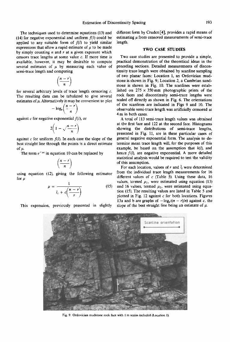
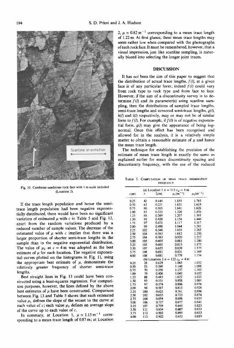
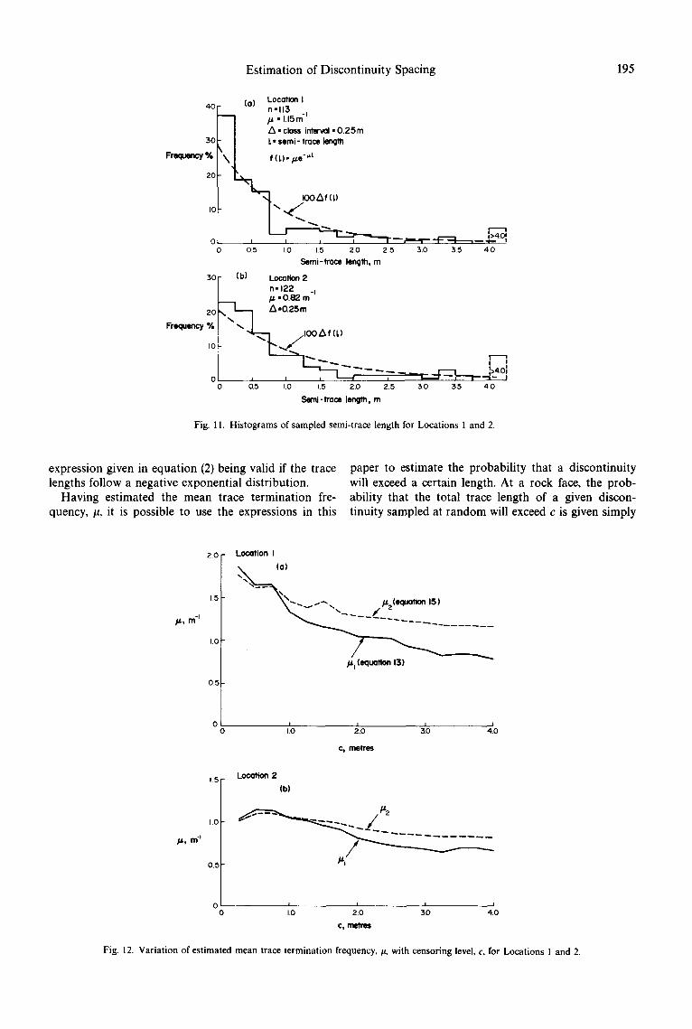
Two case studies are presented to provide a simple, practical demonstration of the theoretical ideas in the preceding sections. Detailed measurements of discontinuity trace length were obtained by scanline sampling of two planar faces: Location 1, an Ordovician mudstone is shown in Fig. 9; Location 2, a Cambrian sandstone is shown in Fig. 10. The scanlines were established on 275 x 350mm photographic prints of the rock faces and discontinuity semi-trace lengths were scaled off directly as shown in Fig. 6. The orientations of the scanlines are indicated in Figs 9 and 10. The observable semi-trace length was artificially censored at 4 m in both cases.

A total of 113 semi-trace length values was obtained at the first face and 122 at the second face. Histograms showing the distributions of semi-trace lengths, presented in Fig. 11, are in these particular cases of general negative exponential form. The analysis to determine mean trace length will, for the purposes of this example, be based on the assumption that h(l), and hence f ( l) , are negative exponential. A more detailed statistical analysis would be required to test the validity of this assumption.

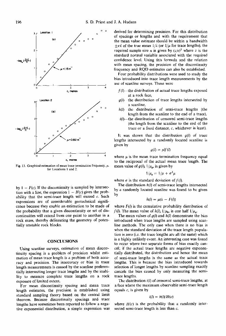
For each location, values of r and li were determined from the individual trace length measurements for 16 different values of c (Table 5). Using these data, 16 values, termed #1, were estimated using equation (13) and 16 values, termed #2, were estimated using equation (15). The resulting values are listed in Table 5 and plotted in Fig. 12 against c for both locations. Figures 13a and b are graphs of -loge((n - r)/n) against c, the slope of the best straight line being an estimate of/~.

Fig. 9. Ordovician mudstone rock face with 1 m scales included (Location 1).

194 S . D . Priest and J. A. Hudson

2,/~ = 0.82 m - ~ corresponding to a mean trace length of 1.22 m. At first glance, these mean trace lengths may seem rather low when compared with the pho tographs of each rock face. It must be remembered, however, that a visual impression, just like scanline sampling, is naturally biased into selecting the longer joint traces.

D I S C U S S I O N

It has not been the aim of this paper to suggest that the distribution of actual trace lengths, f(1), at a given face is of any particular form; indeed f ( l ) could vary from rock type to rock type and from face to face. However, if the aim of a discontinuity survey is to determine f ( l ) and its parameter(s) using scanline sampling, then the distributions of sampled trace lengths, semi-trace lengths and censored semi-trace lengths, 9(1), h(1) and i(l) respectively, may or may not be of similar form to f(/). For example, if f ( / ) is of negative exponential form, 9(1) may give the appearance of being log- normal. Once this effect has been recognised and allowed for in the analysis, it is a relatively simple matter to obtain a reasonable estimate of # and hence the mean trace length.

The technique for establishing the precision of the estimate of mean trace length is exactly the same as explained earlier for mean discontinuity spacing and discontinuity frequency, with the use of the reduced

Fig. 10. Cambrian sandstone rock face with 1 m scale included (Location 2).

If the trace length popula t ion and hence the semi- trace length populat ion had been negative exponentially distributed, there would have been no significant variat ion of estimated p with c in Table 5 and Fig. 12, apart from the r a n d o m variations produced by a reduced number of sample values. The decrease of the estimated value of p with c implies that there was a larger p ropor t ion of shorter semi-trace lengths in the sample than in the negative exponential distribution. The value of ~2 at c = 4 m was adopted as the best estimate of/~ for each location. The negative exponential curves plotted on the his tograms in Fig. 11, using the appropr ia te best estimate of /~, demonstra te the relatively greater frequency of shorter semi-trace lengths.

Best straight lines in Fig. 13 could have been constructed using a least-squares regression. For compar i - son purposes, however, the lines defined by the above best estimates of # have been constructed. Compar i son between Fig. 13 and Table 5 shows that each estimated value/~1 defines the slope of the secant to the curve at each value of c; each value #2 defines an average slope of the curve up to each value of c.

In summary, at Loca t ion 1, / a - - -1 .15m -1 corresponding to a mean trace length of 0.87 m; at Locat ion

TABLE 5. COMPUTATION OF MEAN TRACE TERMINATION FREQUENCY

(a) Location 1 n = 113 c., = 4m c(m) r / /(m) #l(m -l) /a2(m l)

0.25 42 0.144 1.859 1.765 0.50 63 0.221 1.631 1.619 0.75 80 0.305 1.641 1.628 1.00 83 0.325 1.326 1.456 1.25 88 0.369 1.207 1.381 1.50 93 0.420 1.154 1.446 1.75 97 0.471 1.117 1.317 2.00 99 0.498 1.044 1.281 2.25 102 0.548 1.035 1.265 2.50 104 0.583 1.012 1.250 2.75 104 0.583 0.920 1.217 3.00 105 0.605 0.883 1.200 3.25 105 0.605 0.815 1.173 3.50 107 0.655 0.839 1.175 3.75 108 0.681 0.831 1.169 4.00 108 0.681 0.779 1.154

(b) Location 2 n = 122 c,, = 4 m 0.25 28 0.129 1.043 1.032 0.50 53 0.260 1.140 1.098 0.75 70 0.350 1.137 1.103 1.00 79 0.406 1.043 1.052 1.25 88 0.483 1.022 1.035 1.50 93 0.531 0.958 1.001 1.75 97 0.574 0.906 0.976 2.00 98 0.587 0.813 0.928 2.25 100 0.621 0.761 0.896 2.50 102 0.655 0.723 0.874 2.75 104 0.694 0.696 0.855 3.00 106 0.737 0.677 0.841 3.25 107 0.759 0.645 0.823 3.50 111 0.854 0.687 0.833 3.75 113 0.902 0.695 0.833 4.00 113 0.902 0.652 0.819


40

3o Frequency %

20

io

3o

2O Frequency%

ro

o ' i 0 05 I0

[o) Locotion I n-l13 I

l L~ • closs intervol • 0.25m I L" semi- troce length

\ L r ~ f (L).Fe-~L

" ~ . ~ ~ A f l L )

' " - - ' r - - , - , - , _ _ ' , ~ , , 1 - - - ~ ~ - ~ 4 ° 1

0 0.5 I 0 15 2.0 2.5 3.0 3.5 40 Semi-trace length t m

[b) Locotion 2 n-122 # -0 .82 m -I A =0.25 m

~ " 1 ~ / ' ~ .100/k f (k)

-.-. I i

I ~ ' ' " I , , , , - , - - r - - I - - i - I 11,5 2.0 2.5 3.0 3.5 4.0

Semi - trace length, m

Fig. 11. Histograms of sampled semi-trace length for Locations 1 and 2.

expression given in equation (2) being valid if the trace lengths follow a negative exponential distribution.

Having estimated the mean trace termination frequency, ~t, it is possible to use the expressions in this

paper to estimate the probability that a discontinuity will exceed a certain length. At a rock face, the probability that the total trace length of a given discontinuity sampled at random will exceed c is given simply

//., m -I

2.0

15

1.0

05

0 0

Locotion I ~ _ _ (o)

. " ~ ~ . / #2(eCluotion 15 )

P'l (eqtmlion 131

II0 I I 2.0 3i.0 4.0

Ct metres

1.5

IO

#, m t

0.5

Locofion 2 (b)

#l

i 21.0 i i0 LO 3D 4 C~ n l ~

Fig. 12. Variation of estimated mean trace termination frequency, #, with censoring level, c, for Locations 1 and 2.

196 S.D. Priest and J. A. Hudson

-log (--~ L- )

0 0 3 1 - o

0 I 0 4

Location I /

o (i) o o o o o o o

L I I I 2 3

- tog,(n,l~-.)

Loc~lon 2

Q 0 0

( b l

2 o o o

o

I o

o ~ • 0.82 m "t

0 I 1 I I 0 I 2 3 4

c, metros

F i g . 13. G r a p h i c a l e s t i m a t i o n o f m e a n t r a c e t e r m i n a t i o n f r e q u e n c y , / ~ ,

f o r L o c a t i o n s 1 a n d 2.

by 1 - F(c). If the discontinuity is sampled by intersection with a line, the expression 1 - H(c) gives the probability that the semi-trace length will exceed c. Such expressions are of considerable geotechnical significance because they enable an estimation to be made of the probability that a given discontinuity or set of discontinuities will extend from one point to another in a rock mass, thereby delineating the geometry of poten- tially unstable rock blocks.

CONCLUSIONS

Using scanline surveys, estimation of mean discontinuity spacing is a problem of precision whilst estimation of mean trace length is a problem of both accuracy and precision. The inaccuracy or bias in trace length measurements is caused by the scanline preferentially intersecting longer trace lengths and by the inabi- lity to measure complete trace lengths on a rock exposure of limited extent.

For mean discontinuity spacing and mean trace length estimates, the precision is established using standard sampling theory based on the central limit theorem. Because discontinuity spacings and trace lengths have sometimes been reported to follow a negative exponential distribution, a simple expression was

derived for determining precision. For this distribution of spacings or lengths and with the requirement that the mean value estimate should be within a bandwidth +E~ of the true mean 1/2 (or 1//~ for trace lengths), the required sample size n is given by (z/~) 2 where z is the standard normal variable associated with the required confidence level. Using this formula and the relation with mean spacing, the precision of the discontinuity frequency and RQD estimates can also be established.

Four probability distributions were used to study the bias introduced into trace length measurements by the use of scanline surveys. These were

f( / )-- the distribution of actual trace lengths exposed at a rock face,

g(/)--the distribution of trace lengths intersected by a scanline,

h(/)--the distribution of semi-trace lengths (the length from the scanline to the end of a trace),

/(l)--the distribution of censored semi-trace lengths (the length from the scanline to the end of the trace or a fixed distance, c, whichever is least).

It was shown that the distribution g(l) of trace lengths intersected by a randomly located scanline is given by

g(l) = ~ ( t )

where # is the mean trace termination frequency equal to the reciprocal of the actual mean trace length. The mean value of g(l), 1/#g, is given by

1//~g = 1//a + a2#

where tr is the standard deviation off(l). The distribution h(l) of semi-trace lengths intersected

by a randomly located scanline was found to be given by

h(l) = #(1 - F(I))

where F(l) is the cumulative probability distribution of f(l). The mean value of h(l), 1/#h, is one half 1/#g.

The mean values of g(l) and h(l) demonstrate the bias introduced when trace lengths are sampled using scanline methods. The only case when there is no bias is when the standard deviation of the trace length population is zero (i.e. the trace lengths are all the same) which is a highly unlikely event. An interesting case was found to occur where two separate forms of bias exactly can- cel; if the actual trace lengths are negative exponentially distributed, the distribution and hence the mean of semi-trace lengths is the same as the actual trace lengths. This is because the bias introduced towards selection of longer lengths by scanline sampling exactly cancels the bias caused by only measuring the semi- trace lengths.

The distribution i(l) of censored semi-trace lengths, at a face where the maximum observable semi-trace length equals c, is given by

i(l) = h(l)/H(c)

where H(c) is the probability that a randomly intersected semi-trace length is less than c.


Measurements of censored semi-trace length provide an indication of the form of i(l) and hence h(1), g(l) and f(l). The relations between the distributions provide graphical and analytical methods of estimating mean discontinuity trace length from measurements at an exposure where trace length measurements are censored at c.

Data from two rock faces were obtained to illustrate how an unbiased estimate of mean discontinuity trace length can be determined from biased scanline survey measurements.

Acknowledgements--The work described in this paper forms part of continuing research into rock mass geometry carried out as a joint project by the Imperial College of Science and Technology and the Department of the Environment under the guidance of Professor E. T. Brown and Mr J. B. Boden. Dr Hudson is currently working at the Building Research Establishment of the Department of the Environ- ment where the paper was completed and this paper is published by permission of the Director. Some aspects of the work also constituted part of the rock mechanics programme of the Wisconsin Supercon- ductive Energy Storage Project supported by the U.S. Department of Energy and the Wisconsin Electric Utilities Research Foundation. The authors are grateful to Professor D. M. Cruden for his construc- tive criticism of the manuscript.

Received 14 October 1980; in revised form 11 December 1980.

REFERENCES

1. International Society for Rock Mechanics, Commission on Stan- dardization of Laboratory and Field Tests. Suggested methods for the quantitative description of discontinuities in rock masses. Int. J. Rock Mech. Min. Sci. & Geomech. Abstr. 15, 319-368 (1978).

2. Hudson J. A. & Priest S. D. Discontinuity frequency in soils and rocks. (1981). In preparation.

3. La Pointe P. R. & Hudson J. A. Characterising rock mass joint- ing patterns. (1981) In preparation.

4. Cruden D. M. Describing the size of discontinuities. Int. J. Rock Mech. Min. Sci. & Geomech. Abstr. 14, 133-137 (1977).

5. Harper W. M. Statistics, 2nd edn, 330 pp. Macdonald & Evans, Plymouth (1971).

6. Mode E. B. Elements of Probability and Statistics. 356 pp. Pren- tice-Hall, London (1966).

7. Priest S. D. & Hudson J. A. Discontinuity spacings in rock. Int. J. Rock Mech. Min. Sci. & Geomech. Abstr. 13, 135-148 (1976).

8. Hudson J. A. & Priest S. D. Discontinuities and rock mass geometry. Int. J. Rock Mech. Min. Sci. & Geomech. Abstr. 16, 339-362 (1979).

9. Wallis P. F. & King M. S. Discontinuity spacings in a crystalline rock. Int. J. Rock Mech. Min. Sci. & Geomech. Abstr. 17, 63-66 (1980).

10. Barton N., Lien R. & Lunde J. Engineering classification of rock masses for the design of tunnel support. Rock Mech. 6, 189-236 (1974).

11. Bieniawski Z. T. Geomechanics classification of rock masses and its application in tunnelling. Proc. 3rd Int. Congr. on Rock Mech- anics. ISRM, Denver, Vol. IlA, pp. 27-32 (1974).

12. Baecher G. B. & Lanney N. A. Trace length biases in joint surveys. Proe. 19th U.S. Syrup. on Rock Mechanics, Nevada, Vol. i, pp. 56-65 (1978).

13. Baecher G. B., Lanney N. A. & Einstein H. H. Statistical description of rock properties and sampling. Proc. 18th U.S. Syrup. on Rock Mechanics, Colorado, pp. 5C1.1-5C1.8 (1977).

R.M.M.S. 18/3 8

Documents

Estimation of discontinuity spacing and trace length using scanline surveys