Embed Size (px)
Citation preview

EGTEI
EXPERT GROUP ON TECHNO ECONOMIC ISSUES
EGTEI secretariat
30 September 2014
ESTIMATION OF COSTS OF REDUCTION
TECHNIQUES FOR LCP
METHODOLOGY

Report 30-09-2014
2

Report 30-09-2014
3
Table of content
1. Principles of the cost estimation ......................................................................................... 11
1.1. Composition of Costs .................................................................................................. 11
1.1.1. Investment ............................................................................................................... 11
1.1.2. Operating Costs ....................................................................................................... 12
1.2. Adaption of temporal and currency differences ............................................................ 12
1.2.1. Adaption of currency differences .............................................................................. 12
1.2.2. Adaption of temporal differences ............................................................................. 12
1.3. Utility costs .................................................................................................................. 13
2. Boiler Outlet Emission Loads.............................................................................................. 14
2.1. Fuel consumption ........................................................................................................... 14
2.2. Capacity factor ............................................................................................................ 14
2.3. Boiler and Fuel Characteristics .................................................................................... 15
2.3.1. Detailed approach for solid and liquid fuels .............................................................. 16
2.3.1.1. Calculation of fuel lower heating value ................................................................. 17
2.3.1.2. Calculation of carbon-in-ash effect onto flue gas volume rates ............................. 18
2.3.1.3. Calculation of ideal specific flue gas volume rates ................................................ 18
2.3.1.4. Calculation of ash load ......................................................................................... 19
2.3.1.5. Calculation of SO2 load ........................................................................................ 19
2.3.1.6. Calculation of NOx load ........................................................................................ 20
2.3.2. Detailed approach for gaseous fuels ........................................................................ 21
2.3.2.1. Calculation of NOx emissions ............................................................................... 22
2.3.3. General approach .................................................................................................... 22
2.3.4. O2 correction ............................................................................................................ 23
2.4. Integration of Biomass Co-firing .................................................................................. 24
2.4.1. Effect of co-firing on boiler outlet emissions ............................................................. 24
3. Evaluation of NOx abatement techniques ........................................................................... 26
3.1. Primary Measures ....................................................................................................... 26
3.2. Secondary Measures .................................................................................................. 26
3.2.1. Selective Catalytic Reduction................................................................................... 27
3.2.1.1. Pressure drop calculation ..................................................................................... 27

Report 30-09-2014
4
3.2.1.2. Catalyst cost ........................................................................................................ 27
3.2.1.3. Reagent consumption .......................................................................................... 28
3.2.1.4. Additional power consumption .............................................................................. 28
3.2.1.5. Effect of biomass co-firing on SCR ....................................................................... 29
3.2.2. Selective Non Catalytic Reduction ........................................................................... 29
3.2.2.1. Reagent Consumption .......................................................................................... 30
3.2.2.2. Pressure Drop ...................................................................................................... 31
3.2.2.3. Additional power consumption .............................................................................. 31
3.2.2.4. Total costs ............................................................................................................ 31
4. Evaluation of dust abatement techniques ........................................................................... 33
4.1. Introduction ................................................................................................................. 33
4.2. Fabric filter .................................................................................................................. 33
4.2.1. Air-to-Cloth ratio and filtration Area .......................................................................... 34
4.2.2. Fabric filter equipment cost ...................................................................................... 35
4.2.2.1. Baghouse cost ................................................................................. 35
4.2.2.2. Filtering media cost ............................................................................... 36
4.2.2.3. Cage cost ............................................................................................. 37
4.2.3. Fabric filter investment determination ...................................................................... 37
4.2.4. Operating costs........................................................................................................ 38
4.2.4.1. Electricity consumption ......................................................................................... 38
4.2.4.2. Bag replacement ................................................................................. 39
4.2.4.3. By-product disposal or recovery ................................................. 39
4.2.5. Efficiency of PJFF .................................................................................................... 40
4.3. Electro Static Precipitator ............................................................................................ 40
4.3.1. Investment costs ...................................................................................................... 40
4.3.1.1. Bottom up approach for value ..................................................................... 40
4.3.1.2. ESP investment determination ............................................................................. 43
4.3.2. Operating costs........................................................................................................ 46
4.3.2.1. Electricity consumption ......................................................................................... 46
4.3.2.2. SO3 consumption ....................................................................................... 46
4.3.2.3. By-product disposal or recovery ................................................. 47
Report 30-09-2014
5
4.4. Biomass co-firing and liquid fuels ................................................................................ 47
5. Evaluation of SO2 abatement techniques ........................................................................... 49
5.1. LSFO FGD .................................................................................................................. 50
5.1.1. Investment costs ...................................................................................................... 50
5.1.2. Operating costs........................................................................................................ 53
5.1.2.1. Auxiliary electricity ................................................................................................ 53
5.2.1.2. Limestone consumption ....................................................................................... 54
5.2.1.3. By-product, disposal or recovery .......................................................................... 55
5.1.3. Adaptation of costs for installations consuming heavy fuel oil .................................. 56
5.2. Lime spray dryer FGD (LSD FGD) .............................................................................. 57
5.2.1. Investment costs ...................................................................................................... 57
5.2.2. Operating costs........................................................................................................ 59
5.2.2.1. Auxiliary electricity ................................................................................................ 59
5.2.2.2. Lime consumption ................................................................................................ 60
5.2.2.3. By-product, disposal or recovery .......................................................................... 61
5.2.3. Adaptation of costs for installations consuming heavy fuel oil .................................. 62
5.3. Dry FGD ...................................................................................................................... 64
5.3.1. Investment costs ...................................................................................................... 64
5.3.2. Operating costs........................................................................................................ 66
5.3.2.1. Electricity .............................................................................................................. 66
5.3.2.2. Lime consumption ................................................................................................ 66
5.3.2.3. By-products, recovery or disposal ........................................................................ 67
5.2.3.4. Bag replacement .................................................................................................. 67
5.4. Fuel substitution .......................................................................................................... 67
Bibliography ........................................................................................................................... 69
Report 30-09-2014
6
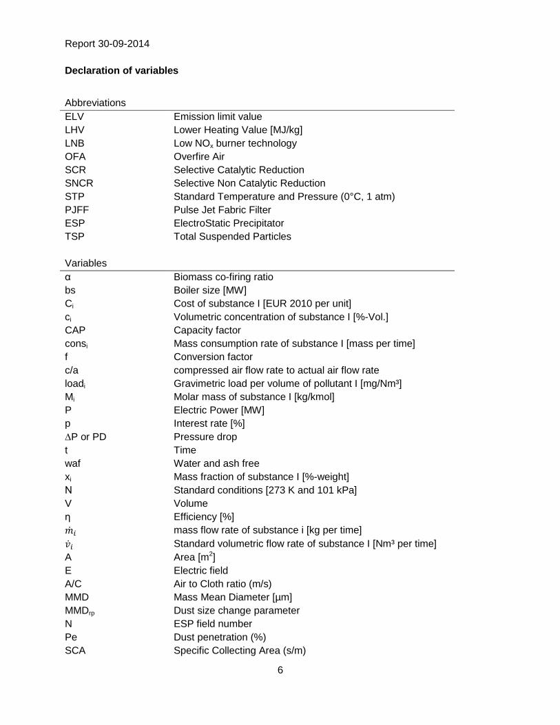
Declaration of variables
Abbreviations
ELV Emission limit value
LHV Lower Heating Value [MJ/kg]
LNB Low NOx burner technology
OFA
SCR
SNCR
Overfire Air
Selective Catalytic Reduction
Selective Non Catalytic Reduction
STP Standard Temperature and Pressure (0°C, 1 atm)
PJFF Pulse Jet Fabric Filter
ESP ElectroStatic Precipitator
TSP Total Suspended Particles
Variables
α
bs
Biomass co-firing ratio
Boiler size [MW]
Ci Cost of substance I [EUR 2010 per unit]
ci
CAP
Volumetric concentration of substance I [%-Vol.]
Capacity factor
consi Mass consumption rate of substance I [mass per time]
f Conversion factor
c/a compressed air flow rate to actual air flow rate
loadi Gravimetric load per volume of pollutant I [mg/Nm³]
Mi Molar mass of substance I [kg/kmol]
P Electric Power [MW]
p
∆P or PD
Interest rate [%]
Pressure drop
t Time
waf Water and ash free
xi Mass fraction of substance I [%-weight]
Ν
V
Standard conditions [273 K and 101 kPa]
Volume
η Efficiency [%]
mass flow rate of substance i [kg per time]
Standard volumetric flow rate of substance I [Nm³ per time]
A Area [m2]
E Electric field
A/C Air to Cloth ratio (m/s)
MMD Mass Mean Diameter [µm]
MMDrp Dust size change parameter
N ESP field number
Pe Dust penetration (%)
SCA Specific Collecting Area (s/m)
Report 30-09-2014
7
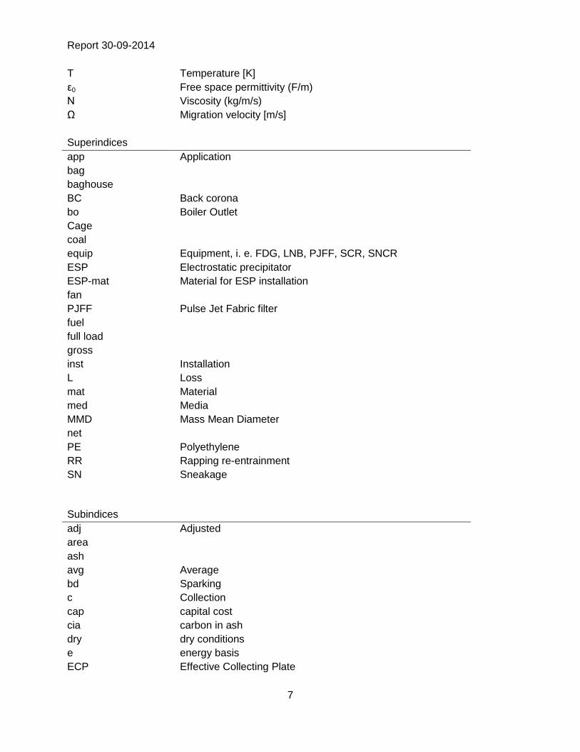
T Temperature [K]
ε0 Free space permittivity (F/m)
Ν Viscosity (kg/m/s)
Ω Migration velocity [m/s]
Superindices
app Application
bag
baghouse
BC Back corona
bo Boiler Outlet
Cage
coal
equip Equipment, i. e. FDG, LNB, PJFF, SCR, SNCR
ESP Electrostatic precipitator
ESP-mat Material for ESP installation
fan
PJFF Pulse Jet Fabric filter
fuel
full load
gross
inst Installation
L Loss
mat Material
med Media
MMD Mass Mean Diameter
net
PE Polyethylene
RR Rapping re-entrainment
SN Sneakage
Subindices
adj Adjusted
area
ash
avg Average
bd Sparking
c Collection
cap capital cost
cia carbon in ash
dry dry conditions
e energy basis
ECP Effective Collecting Plate
Report 30-09-2014
8
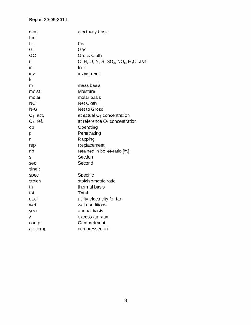
elec electricity basis
fan
fix Fix
G Gas
GC Gross Cloth
i C, H, O, N, S, SO2, NOx, H2O, ash
in Inlet
inv investment
k
m mass basis
moist Moisture
molar molar basis
NC Net Cloth
N-G Net to Gross
O2, act. at actual O2 concentration
O2, ref. at reference O2 concentration
op Operating
p Penetrating
r Rapping
rep Replacement
rib retained in boiler-ratio [%]
s Section
sec Second
single
spec Specific
stoich stoichiometric ratio
th thermal basis
tot Total
ut.el utility electricity for fan
wet wet conditions
year annual basis
λ excess air ratio
comp Compartment
air comp compressed air

Report 30-09-2014
9
Preamble/Foreword
The first international legally binding instrument dealing with air pollution was the UNECE
Convention on Long-range Transboundary Air Pollution (CLRAP) from 1979. This Convention
supplied the framework for the First and Second Sulphur Protocol (1985, 1994), the Protocol on
NOx (1988) and on VOC (1991), with the objective of developing long-term policies to protect
human health and the environment from the effects of air pollution. The most recent one is the
Gothenburg Protocol from 1999, which came into force in May 2005 and has been amended in
May 2012.
The amended Gothenburg Protocol (2012) aims at noticeably reducing acidification,
eutrophication, tropospheric ozone formation and health impact of fine particles (PM2.5) by
setting national emission reduction commitments (% reduction/2005 emissions) for the
responsible pollutants, namely NOx, SO2, NMVOC, NH3 and PM2.5, which have to be achieved
by 2020. The Protocol further contains binding requirements in the form of emission limit values
for both stationary and mobile sources, as well as fuel standards. A specific annex aims at
reducing the emissions of ammonia from agricultural activities. Starting from the critical loads
approach, and addressing several environmental problems and several pollutants
simultaneously, this combined abatement strategy supplied a more cost-effective solution than
treating pollutants or effects separately; that’s why the Gothenburg Protocol is also called “Multi-
pollutants and Multi-effects Protocol”.
Multinational strategies for the reduction of air pollution or greenhouse gases are mainly based
on scenarios generated by means of Integrated Assessment Modelling (IAM). The new national
emission reduction commitments in the amended Gothenburg Protocol were negotiated on the
basis of results obtained by the GAINS (Greenhouse Gas and Air Pollution Interactions and
Synergies) model, developed at the International Institute for Applied System Analysis (IIASA).
GAINS is currently also being used for the revision of the NEC (National Emission Ceiling)
Directive of 2001 by the European Commission.
The GAINS model estimates the internationally cost-optimal allocation of emission reductions.
i.e. it determines where and how much emissions should be reduced to minimize the cost of
removal and still meet pre-selected environmental targets (e.g. desired protection levels for
vegetation, sensible ecosystems or human health) given by critical loads and levels, and
constraints such as maximum allowable costs. Good knowledge of detailed technical and
economic data for all relevant production processes and related abatement options is a crucial
basis for credible IAM.
EGTEI is mandated by UNECE in the scope of the CLRTAP to develop technical and economic
data for relevant processes and related abatement techniques for stationary sources.
The methodology for cost estimation of abatement options of SO2, NOx and TSP (Total
Suspended Particulates) for Large Combustion Plants (LCP) with a thermal capacity of more
than 50 MWth, presented hereafter, aims at providing cost data for the following reduction
techniques applied on large combustion plants using coal, heavy fuel oil and natural gas as well
as biomass in co-combustion with coal.

Report 30-09-2014
10
Only boilers are considered (gas turbines could be examined in the next steps). Reduction
techniques considered are the following ones:
NOx: primary measures, SNCR (Selective Non Catalytic Reduction) and SCR (Selective
Catalytic Reduction),
TSP: electrostatic precipitator (ESP) and fabric filter (FF),
SO2: wet flue gas desulphurisation by limestone forced oxidation (LSFO – Limestone
Forced Oxidation), semi dry (LSD - Lime Spray Dryer) and dry desulphurisation (DSI -
Duct Sorbent Injection). Remark: use of lime is only presented in this report but use of
sodium bicarbonate will be included in the next update of the tool (end 2014).
Costs are estimated for different regulatory objectives in term of ELVs (Emission Limit Values)
assuming one boiler linked to a chimney.
To assist the EGTEI technical secretariat to develop the cost estimations for LCP, a working
group has been set up.
Participants were:
Nicolas Caraman (EDF, France); David Cooling (E’on, United Kingdom); Richard Brandwood
(E’on, United Kingdom); Koen Smekens (ECN, Netherlands); Daniel Ladang (Total/CEFIC,
Belgium); Hélène Lavray (Eurelectric, Belgium), Ivan Jankov (European Commission), Frans
Van AART (KEMA); Tiziano Pigantelli (EGTEI Co-chair); Jean-Guy Bartaire (EGTEI Co-chair) ;
Other experts contributed to deliver information to the EGTEI technical secretariat: the French
group from the Chemical industry Union on coal boilers (chaired by Michel Monzain);
manufacturers of abatement equipment (Hamon, Solvair, GE Air Filtration), operators of
combustion plants.
Report 30-09-2014
11
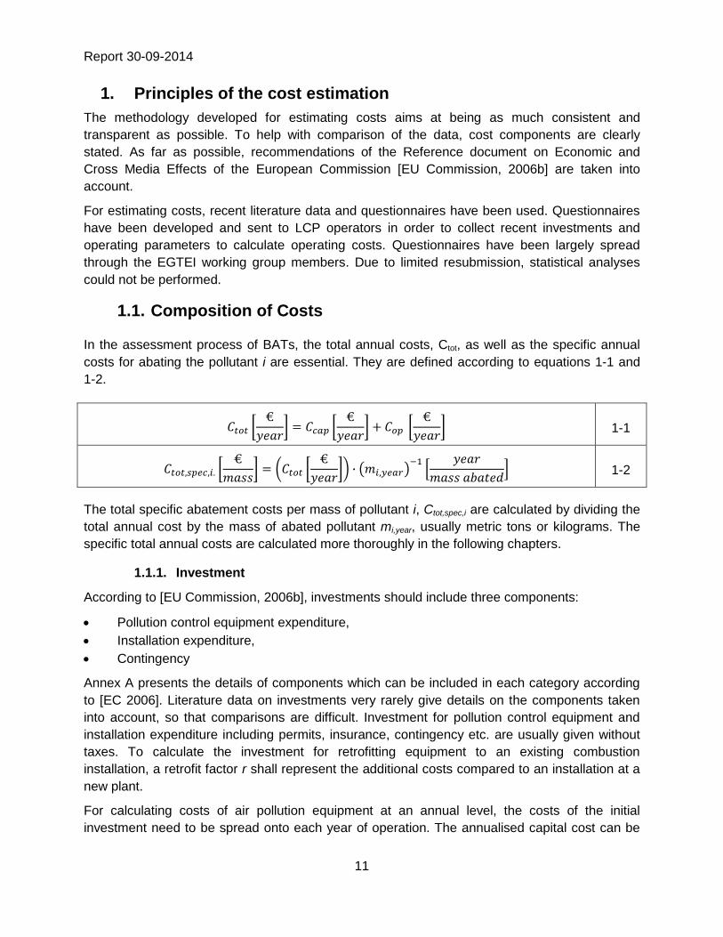
1. Principles of the cost estimation
The methodology developed for estimating costs aims at being as much consistent and
transparent as possible. To help with comparison of the data, cost components are clearly
stated. As far as possible, recommendations of the Reference document on Economic and
Cross Media Effects of the European Commission [EU Commission, 2006b] are taken into
account.
For estimating costs, recent literature data and questionnaires have been used. Questionnaires
have been developed and sent to LCP operators in order to collect recent investments and
operating parameters to calculate operating costs. Questionnaires have been largely spread
through the EGTEI working group members. Due to limited resubmission, statistical analyses
could not be performed.
1.1. Composition of Costs
In the assessment process of BATs, the total annual costs, Ctot, as well as the specific annual
costs for abating the pollutant i are essential. They are defined according to equations 1-1 and
1-2.
1-1
1-2
The total specific abatement costs per mass of pollutant i, Ctot,spec,i are calculated by dividing the
total annual cost by the mass of abated pollutant mi,year, usually metric tons or kilograms. The
specific total annual costs are calculated more thoroughly in the following chapters.
1.1.1. Investment
According to [EU Commission, 2006b], investments should include three components:
Pollution control equipment expenditure,
Installation expenditure,
Contingency
Annex A presents the details of components which can be included in each category according
to [EC 2006]. Literature data on investments very rarely give details on the components taken
into account, so that comparisons are difficult. Investment for pollution control equipment and
installation expenditure including permits, insurance, contingency etc. are usually given without
taxes. To calculate the investment for retrofitting equipment to an existing combustion
installation, a retrofit factor r shall represent the additional costs compared to an installation at a
new plant.
For calculating costs of air pollution equipment at an annual level, the costs of the initial
investment need to be spread onto each year of operation. The annualised capital cost can be

Report 30-09-2014
12
calculated according to 1-3 with the parameters p (interest rate) and n (equipment technical or
economic lifetime).
1-3
In case of unknown life time of the control equipment the lifetime is assumed to be equal to the
lifetime of the power plant.
1.1.2. Operating Costs
Total operating costs are composed of fixed and variable operating costs.
1-4
The fixed operating costs, Cop,fix are usually calculated as a percentage of the unit investment
and include costs such as maintenance, insurance, wages1, etc.
Variable operating costs Cop,var enclose costs for utilities such as electricity, waste disposal,
reagents etc. The costs for disposal may be negative in case of the possibility of selling the
residues (i.e. fly ash or gypsum).
, unit {equipment, reagent, electricity, disposal} 1-5
1.2. Adaptation of temporal and currency differences
1.2.1. Adaptation of currency differences
Currency conversion to EURO from literature values in foreign currencies are done, if available
at the reported conversion rates and stated explicitly. If no currency conversion rate was given,
the yearly average of the conversion rate was determined and used for calculation.
1.2.2. Adaptation of temporal differences
Due to the time value of money, investment and costs cannot be compared without integrating
the temporal aspect. To enable the comparison of costs or investments from different years,
various indexes have been developed. One of these indexes, the Chemical Engineering Plant
1 It was the objective of the EGTEI technical secretariat to specify wage costs independently, when the revision of the
cost methodology started. The working group decided to follow the common rules and include them in fixed operating costs finally due to lack of data.
Report 30-09-2014
13
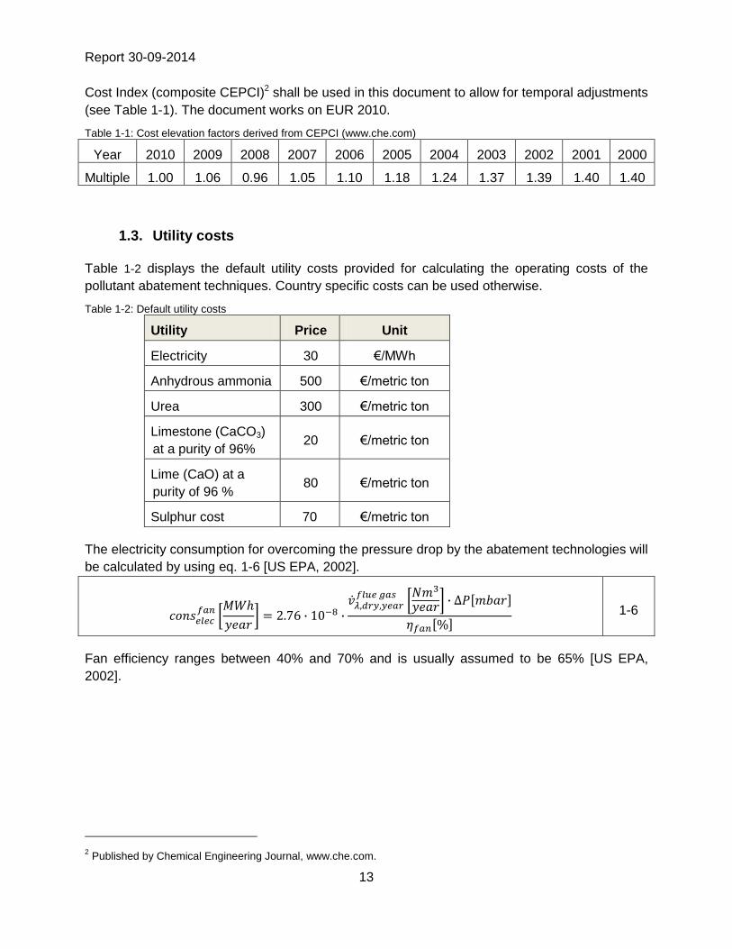
Cost Index (composite CEPCI)2 shall be used in this document to allow for temporal adjustments
(see Table 1-1). The document works on EUR 2010.
Table 1-1: Cost elevation factors derived from CEPCI (www.che.com)
Year 2010 2009 2008 2007 2006 2005 2004 2003 2002 2001 2000
Multiple 1.00 1.06 0.96 1.05 1.10 1.18 1.24 1.37 1.39 1.40 1.40
1.3. Utility costs
Table 1-2 displays the default utility costs provided for calculating the operating costs of the
pollutant abatement techniques. Country specific costs can be used otherwise.
Table 1-2: Default utility costs
Utility Price Unit
Electricity 30 €/MWh
Anhydrous ammonia 500 €/metric ton
Urea 300 €/metric ton
Limestone (CaCO3)
at a purity of 96% 20 €/metric ton
Lime (CaO) at a
purity of 96 % 80 €/metric ton
Sulphur cost 70 €/metric ton
The electricity consumption for overcoming the pressure drop by the abatement technologies will
be calculated by using eq. 1-6 [US EPA, 2002].
1-6
Fan efficiency ranges between 40% and 70% and is usually assumed to be 65% [US EPA,
2002].
2 Published by Chemical Engineering Journal, www.che.com.
Report 30-09-2014
14
2. Boiler Outlet Emission Loads
Combining the parametric set of boiler characteristics with the parametric set of fuel composition
enables to calculate boiler outlet emission loads for all necessary pollutants. Hereby, the
integration of information on boiler size and operating hours per year is provided, in order to
derive yearly emission loads for the economic assessment.
Step 1 (subchapter 2.1) provides formulae for boiler capacity in terms of throughput.
Step 2 (subchapter 2.2) derives the boiler capacity factor.
Step 3 (subchapter 2.3) derives the volumetric boiler outlet emissions for given fuels.
In step 4 (2.4), formulae are given for integrating the effects of using different fuels within one
boiler, for example the co-firing of low rank coals or biomass. According to the core idea of
evaluating emission abatement techniques upon available information, calculations for boiler
outlet emission loads will be provided on the basis of detailed, as well as, broad data.
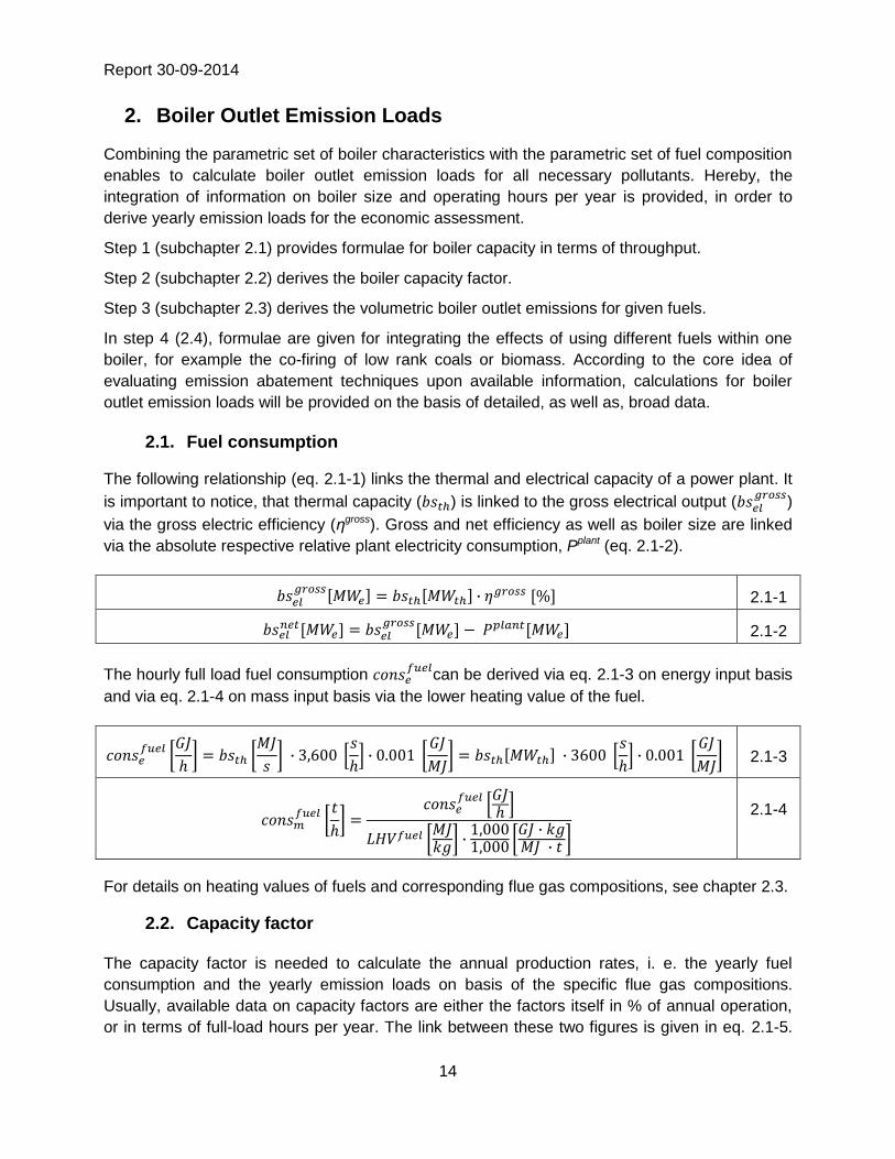
2.1. Fuel consumption
The following relationship (eq. 2.1-1) links the thermal and electrical capacity of a power plant. It
is important to notice, that thermal capacity ( ) is linked to the gross electrical output (
)
via the gross electric efficiency (ηgross). Gross and net efficiency as well as boiler size are linked
via the absolute respective relative plant electricity consumption, Pplant (eq. 2.1-2).
2.1-1
2.1-2
The hourly full load fuel consumption
can be derived via eq. 2.1-3 on energy input basis
and via eq. 2.1-4 on mass input basis via the lower heating value of the fuel.
2.1-3
2.1-4
For details on heating values of fuels and corresponding flue gas compositions, see chapter 2.3.
2.2. Capacity factor
The capacity factor is needed to calculate the annual production rates, i. e. the yearly fuel
consumption and the yearly emission loads on basis of the specific flue gas compositions.
Usually, available data on capacity factors are either the factors itself in % of annual operation,
or in terms of full-load hours per year. The link between these two figures is given in eq. 2.1-5.

Report 30-09-2014
15
For the further calculations, the number of full-load hours per year will be needed (chapter 2.3).
The methodology does not account for additional emissions or reduced efficiency due to low
load operations, so that the total operating hours and the corresponding load vector can be
simplified to the annual full-load operating hours per year.
2.1-5
Table 2.1-1 shows full-load operating hours for typical power plant classifications and can be
used for orientation.
Table 2.1-1: Plant classification according to Strauß (2006)
Plant Classification Full-load hours per year
Base load I > 7,000 h/a
Base load II 5,000 - 7,000 h/a
Medium Load 2,000 - 5,000 h/a
Peak Load < 2,000 h/a
2.3. Boiler and Fuel Characteristics
The aim of this subchapter is to derive the specific flue gas composition at boiler outlet on the
basis of a given fuel specification. Depending on the detail of information about fuels used, a
detailed and a rather general approach can be used. Solid and liquid fuels use a common
methodology (subchapters 2.3.1), whereas for gases, a somewhat different approach has to be
applied (subchapter 2.3.2). Solid and liquid fuels are usually characterised by mass analyses, i.
e. elementary shares of carbon, hydrogen, sulphur, etc., natural gases are usually characterised
by component volume fractions (CH4, C2H6, etc.).
At first, certain parameters, which characterise the combustion process, need to be specified.
These operating parameters depend mainly on construction characteristics and plant operation.
These factors are the excess air ratio (λ), the carbon-in-ash content (xcia) and the fraction of ash
retained in the boiler, i. e. the ratio of bottom ash to total ash. The ash-related parameters will be
discussed and handled in subchapter 2.3.1.4. Combustion of natural gas usually emits no
particulate matter, therefore TSP emission can be neglected. For excess air ratios, Strauß
[Strauß 2006] provides a range of typical ratios according to fuel and combustion technology for
coal.

Report 30-09-2014
16
Table 2.1-2: Literature values for excess air ratios (Strauß, 2006)
Fuel / Technology Typical values for λ
Oil 1.03-1.15
Gas 1.05-1.10
Coal
dry bottom 1.2-1.3
wet bottom 1.15-1.25
grate 1.3-1.4
2.3.1. Detailed approach for solid and liquid fuels
Basis of this detailed approach is a fuel composition from elementary analysis of the water and
ash free (waf) fuel, providing mass fractions of the relevant elementary components carbon (C),
hydrogen (H), oxygen (O), nitrogen (N) and sulphur (S)3 (CHONS). Assuming complete
combustion, specific flue gas volumes as well as the lower heating value can be calculated from
these CHONS data by mass balancing. Hereby, the following assumptions are made:
- Full oxidation of carbon to CO2, no existence of CO or elementary carbon
- No nitrogen oxidation to nitrogen oxides
- Full oxidation of sulphur to SO2, no existence of SO3 and higher sulphur oxides or
elementary sulphur
Large combustion plants usually emit CO, SO3 and nitrogen oxides at mg/Nm³ levels – the error
introduced by these assumptions is however rather small. Nevertheless, if values for NOx, CO
and SO3 exist or are assumed, adjustment calculations can be added. Adjustments for
elementary carbon can be meaningful, especially for PM emission load analysis and will
therefore be performed in subchapter 2.3.1.2.
3 As this composition is water- and ash-free, the CHONS mass fractions should add up to 100%.
Report 30-09-2014
17
Table 2.1-3 shows some exemplary CHONS data for various hard coals from online literature
surveys.
Table 2.1-4 shows equivalent data for typical liquid fuels used in large combustion plants. The
exact ratios of the oils depend upon source and preparation, as these combustion fuels are not
usually used in its raw state, but rather as a product of refining. In addition, HHV (Higher heating
value) or LHV (Lower Heating Value) are well known characteristic figures and therefore, do not
need to be calculated, as done for coal in equation 2.1-6.

Report 30-09-2014
18
Table 2.1-3: Exemplary data for some important hard coals used in the LCP sector
Coal Mine Country Elementary composition (waf)
Ash Moist. C H O N S
Cerrejon Columbia 83.4 4.95 9.47 1.37 0.81 8.41 11.83
Middelburg South Africa 82.44 5.02 10.43 1.38 0.73 13.55 7.42
APC Australia 88.58 4.73 4.22 1.46 1.00 11.12 10.27
Bachatsky Russia 87.03 4.66 5.36 2.58 0.37 9.52 10.22
Bailey USA 84.35 5.58 6.05 2.09 1.74 7.00 7.00
Blackwater Australia 86.48 4.93 5.71 1.95 0.93 14.16 8.79
Douglas South Africa 83.30 5.11 9.47 1.42 0.70 13.75 7.65
Elandsfontein South Africa 88.16 4.86 4.91 1.43 0.64 12.74 9.00
Kleinkopje South Africa 85.02 4.74 7.33 2.19 0.72 14.49 7.71
Kromdraai South Africa 81.85 5.03 10.81 1.36 0.95 13.36 7.79
Table 2.1-4: Exemplary data for some important types of liquid fuels
Liquid fuel type HHV
[MJ/kg]
Elementary composition (waf) Ash Moist.
C H O N S4
Crude Oil n/a 83-87 10-14 0.05-
1,5 0.1-2 0.05-6 <1 <0.1
Gasoline 45.7 87 13 n/a n/a n/a n/a n/a
Diesel 47.0 84-86 13-15 n/a n/a <0.02 n/a n/a
Biodiesel 40.0 77 12 11 n/a 0.01 n/a n/a
Heavy Fuel Oil 43.0 86-88 8-10 n/a n/a 1-5 0.50 0.1
2.3.1.1. Calculation of fuel lower heating value
The lower heating value of a fuel can be derived upon its CHONS-characteristics
according to eq. 2.1-6 [Strauß 2006].
2.1-6
4 Commercial fuel oil, especially heavy fuel oil sulphur content varies strongly, as it is determined by refinery
operations. Typically, heavy fuel oil can be separated into low sulphur (<0.5%), medium (0.5-2%) and high sulphur (>2%-vol.) heavy fuel oil.

Report 30-09-2014
19
2.3.1.2. Calculation of carbon-in-ash effect onto flue gas volume rates
The carbon-in-ash fraction xcia represents the part of total carbon input, which will not be
oxidised and therefore not turned into flue gases. Therefore it has to be subtracted from the
carbon mass fraction, which will be used in the calculation of specific flue gas volumes. In
general, the carbon-in-ash content varies and depends on fuel as well as on combustion
characteristics. Standards for fly-ash usage in the construction industry (mainly road industry)
limit the carbon-in-ash content to a maximum of 7% weight. Above this limit, fly-ash cannot be
sold to this industry and needs to be land filled at a high cost. Therefore, power plants usually
operate below 7%, mostly between 2% and 5% [EGTEI 2013]. Eq. 2.1-7 and 2.1-8 show the
necessary adjustments made to carbon (xC,adj) and to ash (xash+C).
2.1-7
2.1-8
2.3.1.3. Calculation of ideal specific flue gas volume rates
Total flue gas volume consists of combustion products, nitrogen from combustion air and oxygen
due to the use of excess air. For calculating the flue gas from the elementary CHONS-
composition, Strauß [Strauß 2006] provides eq. 2.1-9, for calculating the necessary combustion
air eq. 2.1-10 and for calculating the specific flue gas volume flow at the excess air ratio eq.
2.1-11. Herein, xi represents the element’s mass fractions of the elementary analysis but
corrected for ash and water5.
2.1-9
2.1-10
2.1-11
The moisture content of the combustion air has been neglected, but could be integrated, if
required by adjusting in adding the moisture volume . The wet flue gas
volume is important for calculating operating costs which are based on actual flue gas volume
flow including moisture, such as for costs of pressure drop. Emission limit values (ELVs) on the
other hand, are defined as emission loads (weight) per dry flue gas volume at standard
5 Elementary analyses are usually provided free of water and ash (waf). For the following calculations, the mass
fractions need to regard the water and ash masses, therefore xi need to be corrected, if given at waf-level.

Report 30-09-2014
20
conditions (0°C and 1 atm, resp. 273 K and 1.013 bar) and a given reference oxygen
concentration. Therefore, it is important to calculate the moisture content of the flue gas and to
differentiate between the wet and dry flue gas volume flows
and
(eq. 2.1-13).
The moisture volume can be derived from fuel moisture (given as mass fraction)
and from fuel hydrogen content (from elementary analysis of the water and ash-free
fuel) , see eq. 2.1-12. The constant is the specific volume of 1,000 mol (1 kmol) of an
ideal gas at standard temperature and pressure (1 atm, 0°C), 22.414 Nm³/kmol.
2.1-12
2.1-13
2.3.1.4. Calculation of ash load
To calculate the ash load of the flue gas, it shall be assumed, that fuel ash will neither be
gasified nor the oxidation states of the ash components changed (and thereby the mass in- or
decreased). The ash either will leave the boiler as fly ash or as bottom ash. The ratio fly/bottom
ash is depending on boiler and combustion characteristics and cannot be generalised.
Therefore, either plant or literature data is needed. As seen in eq. 2.1-14, the fly ash load can be
derived by dividing the specific fly ash mass by the specific dry flue gas volume flow. As it is
assumed, that the ash mass neither in- nor decreases, total fly ash is the difference between
total ash input (from the fuel) and ash, which is retained in the boiler.
2.1-14
2.1-15
2.3.1.5. Calculation of SO2 load
As mentioned, it shall be assumed that all sulphur shall be oxidized to SO2. SO3 loads are
usually <5% of SO2 emissions, therefore the calculation difference is small. Furthermore, sulphur
Report 30-09-2014
21
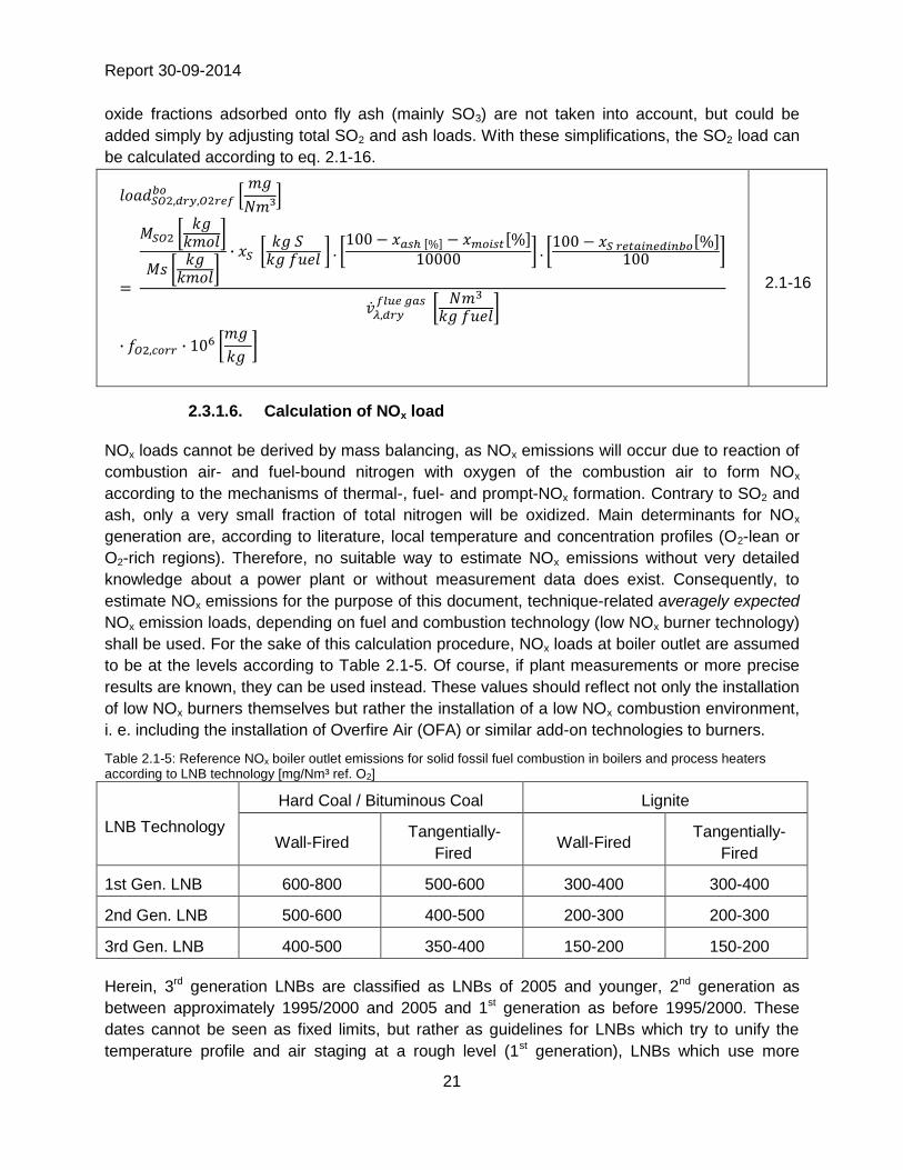
oxide fractions adsorbed onto fly ash (mainly SO3) are not taken into account, but could be
added simply by adjusting total SO2 and ash loads. With these simplifications, the SO2 load can
be calculated according to eq. 2.1-16.
2.1-16
2.3.1.6. Calculation of NOx load
NOx loads cannot be derived by mass balancing, as NOx emissions will occur due to reaction of
combustion air- and fuel-bound nitrogen with oxygen of the combustion air to form NOx
according to the mechanisms of thermal-, fuel- and prompt-NOx formation. Contrary to SO2 and
ash, only a very small fraction of total nitrogen will be oxidized. Main determinants for NOx
generation are, according to literature, local temperature and concentration profiles (O2-lean or
O2-rich regions). Therefore, no suitable way to estimate NOx emissions without very detailed
knowledge about a power plant or without measurement data does exist. Consequently, to
estimate NOx emissions for the purpose of this document, technique-related averagely expected
NOx emission loads, depending on fuel and combustion technology (low NOx burner technology)
shall be used. For the sake of this calculation procedure, NOx loads at boiler outlet are assumed
to be at the levels according to Table 2.1-5. Of course, if plant measurements or more precise
results are known, they can be used instead. These values should reflect not only the installation
of low NOx burners themselves but rather the installation of a low NOx combustion environment,
i. e. including the installation of Overfire Air (OFA) or similar add-on technologies to burners.
Table 2.1-5: Reference NOx boiler outlet emissions for solid fossil fuel combustion in boilers and process heaters according to LNB technology [mg/Nm³ ref. O2]
LNB Technology
Hard Coal / Bituminous Coal Lignite
Wall-Fired Tangentially-
Fired Wall-Fired
Tangentially-
Fired
1st Gen. LNB 600-800 500-600 300-400 300-400
2nd Gen. LNB 500-600 400-500 200-300 200-300
3rd Gen. LNB 400-500 350-400 150-200 150-200
Herein, 3rd generation LNBs are classified as LNBs of 2005 and younger, 2nd generation as
between approximately 1995/2000 and 2005 and 1st generation as before 1995/2000. These
dates cannot be seen as fixed limits, but rather as guidelines for LNBs which try to unify the
temperature profile and air staging at a rough level (1st generation), LNBs which use more
Report 30-09-2014
22
smooth air and fuel staging approaches (2nd generation) and very new LNBs which have been
optimized according to modern CFD simulations and other technical simulation tools for a
minimum of NOx formation.
Table 2.1-6: Reference NOx boiler outlet emissions for liquid fossil fuel combustion in boilers according to LNB
technology in mg/Nm³ at 3%-vol. O2 [EU COMMISSION, 2013]
oil fired units
uncontrolled 800 - 1000
single primary measures 400 - 500
multiple primary measures < 400
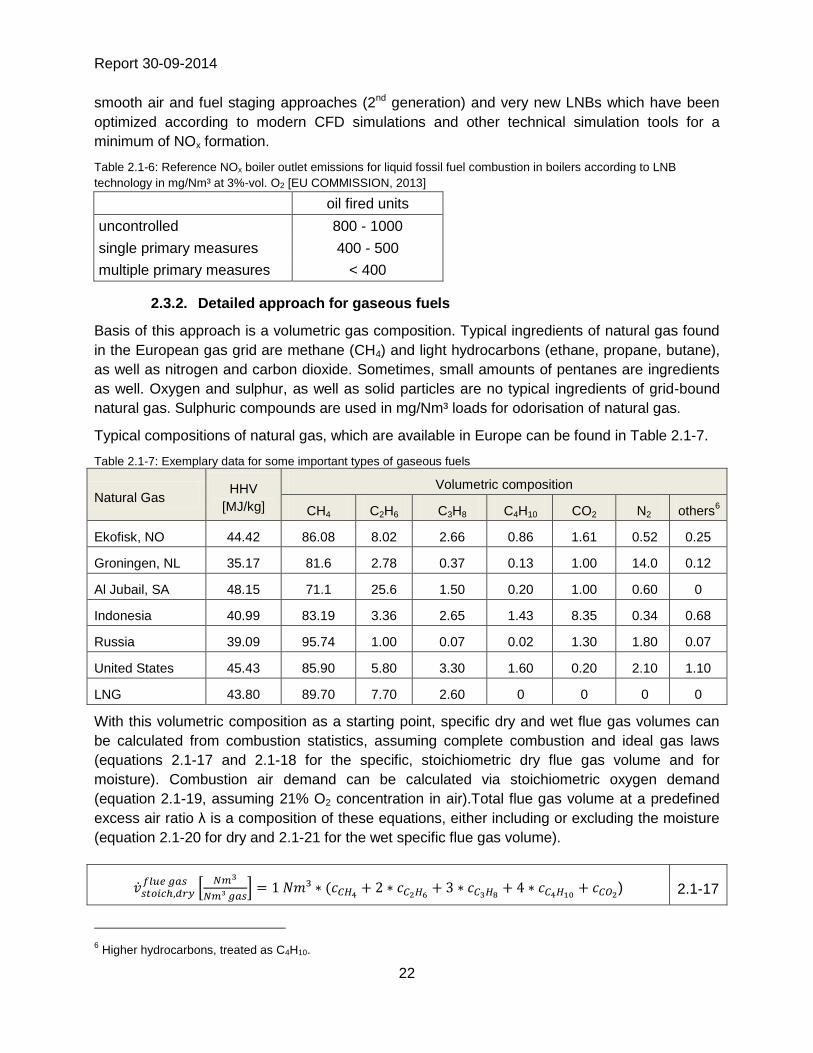
2.3.2. Detailed approach for gaseous fuels
Basis of this approach is a volumetric gas composition. Typical ingredients of natural gas found
in the European gas grid are methane (CH4) and light hydrocarbons (ethane, propane, butane),
as well as nitrogen and carbon dioxide. Sometimes, small amounts of pentanes are ingredients
as well. Oxygen and sulphur, as well as solid particles are no typical ingredients of grid-bound
natural gas. Sulphuric compounds are used in mg/Nm³ loads for odorisation of natural gas.
Typical compositions of natural gas, which are available in Europe can be found in Table 2.1-7.
Table 2.1-7: Exemplary data for some important types of gaseous fuels
Natural Gas HHV
[MJ/kg]
Volumetric composition
CH4 C2H6 C3H8 C4H10 CO2 N2 others6
Ekofisk, NO 44.42 86.08 8.02 2.66 0.86 1.61 0.52 0.25
Groningen, NL 35.17 81.6 2.78 0.37 0.13 1.00 14.0 0.12
Al Jubail, SA 48.15 71.1 25.6 1.50 0.20 1.00 0.60 0
Indonesia 40.99 83.19 3.36 2.65 1.43 8.35 0.34 0.68
Russia 39.09 95.74 1.00 0.07 0.02 1.30 1.80 0.07
United States 45.43 85.90 5.80 3.30 1.60 0.20 2.10 1.10
LNG 43.80 89.70 7.70 2.60 0 0 0 0
With this volumetric composition as a starting point, specific dry and wet flue gas volumes can
be calculated from combustion statistics, assuming complete combustion and ideal gas laws
(equations 2.1-17 and 2.1-18 for the specific, stoichiometric dry flue gas volume and for
moisture). Combustion air demand can be calculated via stoichiometric oxygen demand
(equation 2.1-19, assuming 21% O2 concentration in air).Total flue gas volume at a predefined
excess air ratio λ is a composition of these equations, either including or excluding the moisture
(equation 2.1-20 for dry and 2.1-21 for the wet specific flue gas volume).
) 2.1-17
6 Higher hydrocarbons, treated as C4H10.

Report 30-09-2014
23
2.1-18
2.1-19
2.1-20
2.1-21
Higher heating value is typically supplied with the gas composition, as it is the billing unit.
Sulphur and particulate matter emissions are no concern of natural gas combustion and can be
neglected.
2.3.2.1. Calculation of NOx emissions
For NOx emissions, the same approach as for solid and liquid fuels has to be taken due to the
same reasons. Table 2.1-8 provides some typical NOx boiler outlet emissions, which can be found
in literature.
Table 2.1-8: Reference NOx boiler outlet emissions for g fossil fuel combustion in boilers according to LNB technology in mg/Nm³ at 3%-vol. O2 [EU Commission, 2013]
gas fired units
uncontrolled 150 - 400
single primary measures 75 - 150
multiple primary measures < 75
2.3.3. General approach
The more general approach can be used when no information on the elementary fuel
composition is known. Important input parameters are
Specific flue gas volume (Nm³/kg fuel)
Sulphur content of fuel (%-weight)
Ash and moisture content of fuel (%-weight)
Usually, only the first parameter may be unknown, as the other parameters are essential for
determining the coal quality. Strauß [Strauß 2006] provides a rough estimation of the flue gas
factor and combustion air volume flow only using the LHV as input (eq. 2.1-22 and 2.1-23). It is
important to note, that eq. 2.1-22 and 2.1-23 are only valid for coal. For heating oil and gas,
equations 2.1-24 to 2.1-27 are given. The equations for natural gas require the gas to be
expressed as weight input. Conversion from volumetric to weight input has to be done by
dividing with the mass density of natural gas. If no specific density is known, general density
values of 0.80 to 0.85 kg/Nm³ can be used instead. NOx values have to be determined to the
same way, as done for the detailed approach (subchapter 2.3.1.6).

Report 30-09-2014
24
2.1-22
2.1-23
2.1-24
2.1-25
2.1-26
2.1-27
2.3.4. O2 correction
Adjusting the oxygen concentration of flue gases is necessary, as emission limit values (ELV)
are in general expressed at so called reference oxygen concentrations. Table 1-3 shows the O2
reference concentrations, ELVs are expressed in the amended Gothenburg Protocol of the
Convention on Long-Range Transboundary Air Pollution. It has to be noted that these reference
concentrations may vary from legislation to legislation.
Table 2.1-9: Reference O2 concentrations according to the amended Gothenburg Protocol
Fuel Reference O2
concentration
Solid fuels 6%-Vol.
Liquid fuels 3%-Vol.
Gaseous fuels in boilers
and process heaters
3%-Vol.
Liquid and gaseous fuels
in gas turbines
15%-Vol.
First, the actual oxygen concentration has to be calculated (eq. 2.1-28). Second, the correction
from actual to reference concentration can be done (eq. 2.1-29).
2.1-28

Report 30-09-2014
25
2.1-29
2.4. Integration of Biomass Co-firing
Biomass can be co-fired via three different methods: direct, indirect and parallel co-firing. In this
methodology only direct co-combustion is considered. This assumption needs to be made in
order to be able to analyse the effect of biomass co-combustion on a given unit, which may co-
combust biomass or may alternatively fire purely fossil fuels. Both other types of co-combustion
would require modifications in fuel preparation and injection into the furnace, so that substantial
investments need to be made. Typical co-firing ratios using the method of direct co-firing reach
up until 20% on a mass-basis [ECN 2013].
Regarding the type of biomass only wood is included. Co-firing of straw and other biomass types
is less common than of wood and requires more cautioness with regard to additional flue gas
components (chlorine, fluorine and higher contents of alkaline metals) and their effects onto the
combustion, the ash and gypsum as well as SCR deactivation. In Table 2.1-10 the elemental
composition of different exemplary wood types are given.
Table 2.1-10: Exemplary elemental composition of different wood types [Bunbury, 1925]
Wood type Composition of exemplary biomass (water and ash free, waf)
C H O N
Oak 50,64 6,23 41,85 1,28
Beech 50,89 6,07 42,11 0,93
Birch 50,61 6,23 42,04 1,12
Pine 51,39 6,11 41,56 0,94
Spruce 51,39 6,11 41,56 0,94
2.4.1. Effect of co-firing on boiler outlet emissions
The effect of firing up to 20% biomass (mass-basis) onto the boiler outlet emissions will be
discussed in the following. The following variables are subject to changes:
- Specific flue gas volume per kilogram of fuel
- SO2 emission load
- TSP emission load
- NOx emission load
The first three effects can be integrated using already described formulae for coal combustion,
as biomass features the same ingredients as coal. For calculating the emission load
from biomass co-firing, first the emissions for both pure coal and pure biomass combustion are
Report 30-09-2014
26
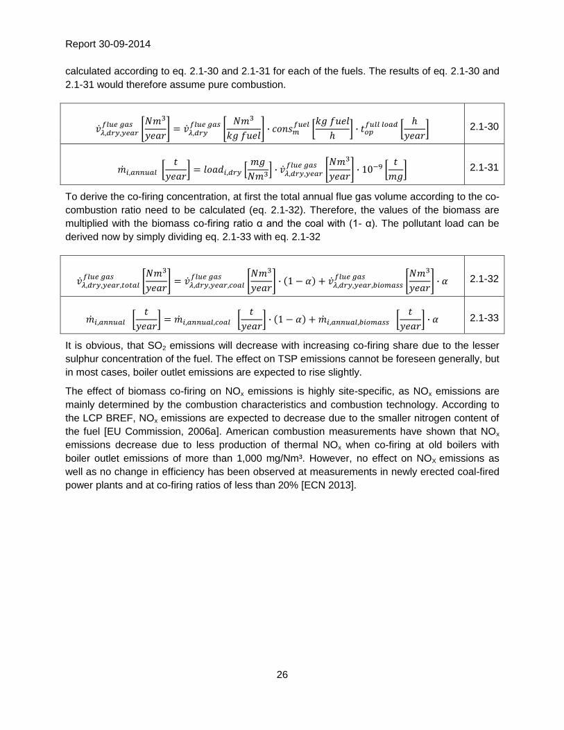
calculated according to eq. 2.1-30 and 2.1-31 for each of the fuels. The results of eq. 2.1-30 and
2.1-31 would therefore assume pure combustion.
2.1-30
2.1-31
To derive the co-firing concentration, at first the total annual flue gas volume according to the co-
combustion ratio need to be calculated (eq. 2.1-32). Therefore, the values of the biomass are
multiplied with the biomass co-firing ratio α and the coal with (1- α). The pollutant load can be
derived now by simply dividing eq. 2.1-33 with eq. 2.1-32
2.1-32
2.1-33
It is obvious, that SO2 emissions will decrease with increasing co-firing share due to the lesser
sulphur concentration of the fuel. The effect on TSP emissions cannot be foreseen generally, but
in most cases, boiler outlet emissions are expected to rise slightly.
The effect of biomass co-firing on NOx emissions is highly site-specific, as NOx emissions are
mainly determined by the combustion characteristics and combustion technology. According to
the LCP BREF, NOx emissions are expected to decrease due to the smaller nitrogen content of
the fuel [EU Commission, 2006a]. American combustion measurements have shown that NOx
emissions decrease due to less production of thermal NOx when co-firing at old boilers with
boiler outlet emissions of more than 1,000 mg/Nm³. However, no effect on NOX emissions as
well as no change in efficiency has been observed at measurements in newly erected coal-fired
power plants and at co-firing ratios of less than 20% [ECN 2013].

Report 30-09-2014
27
3. Evaluation of NOx abatement techniques
For abating NOX emissions primary and secondary measures can be applied. Primary measures
aim at reducing the amount of NOx formed during combustion by optimising boiler or turbine
parameters with respect to emissions. Secondary measures include reagents that reduce NOx.
In the following paragraphs, the operating costs for NOx abatement techniques are calculated.
3.1. Primary Measures
As primary measure for reducing NOx emissions low NOx Burners (LNB) are defined to be state
of the art. These are designed to control air mixing at each burner in order to create larger and
more branched flames and therefore to reduce NOx formation. Plants without LNBs under IPPC
are rather rare. Therefore, only LNBs are considered in this methodology.
To calculate the total costs per year of primary measures and the specific NOx reduction costs
the following equations can be used.
3-1
3-2
3-3
The investment for a LNB is given by the specific investment per kWth of the LCP (see Annex A)
multiplied with the installed thermal capacity. The fixed operating costs are calculated with the
factor for fixed operating and management costs (see equation no. 3-3). According to equation
1-3 the capital costs for LNB can be calculated as in equation no.3-2 by multiplying investment
and interest rate. As the variable operating costs are zero, total costs for the LNB are calculated
according to eq. 3-4.
3-4
The specific NOX abatement cost can then be calculated by dividing the total cost for LNB by the
total NOX emissions abated from upgrading primary measures.
3.2. Secondary Measures
The most common secondary measures are Selective Catalytic Reduction (SCR) and Selective
Non Catalytic Reduction (SNCR). Secondary measures abate NOx by reducing NO and NO2 to
pure N2 and water (plus CO2 in the case of urea) with the use of appropriate reagents such as
ammonia or urea.

Report 30-09-2014
28
3.2.1. Selective Catalytic Reduction
SCRs are mostly built up of multiple layers and use a catalyst to improve the abatement
efficiency. In the following subchapters the operating properties are described and included in
the calculation of the operating costs of SCRs.
3.2.1.1. Pressure drop calculation
A SCR is built up of multiple layers, which influence the pressure drop significantly. Additionally
to the pressure drop of each layer, the pressure drop of injection and mixing as well for the
casing itself contribute to the necessary electricity and, therefore, the electricity cost. The total
pressure drop of an SCR can be calculated by summarizing the above mentioned influencing
factors.
3-5
The calculation of the electricity costs which occur to overcome the pressure drop is calculated
in chapter 3.2.1.4.
3.2.1.2. Catalyst cost
The costs for the catalyst are dependent on the catalyst volume, catalyst lifetime and catalyst
management strategy (number of and interval between catalyst regeneration).
For these calculations a reference SCR unit may have three active and one spare layer. These
can be regenerated after a certain time which leads to a number of possible catalyst
regenerations. If no regeneration of the catalyst is done then the lifetime is mostly reduced. The
choice if the catalyst is regenerated or not lies by the operator of the plant
3-6
3-7
3-8
Data from literature, previous EGTEI information and LCP operators are given in Table 3-1 as a
benchmark. The lifetime is strongly dependent on the catalyst management strategy and the fuel
characteristics (heavy metals, biomass etc.).
Report 30-09-2014
29
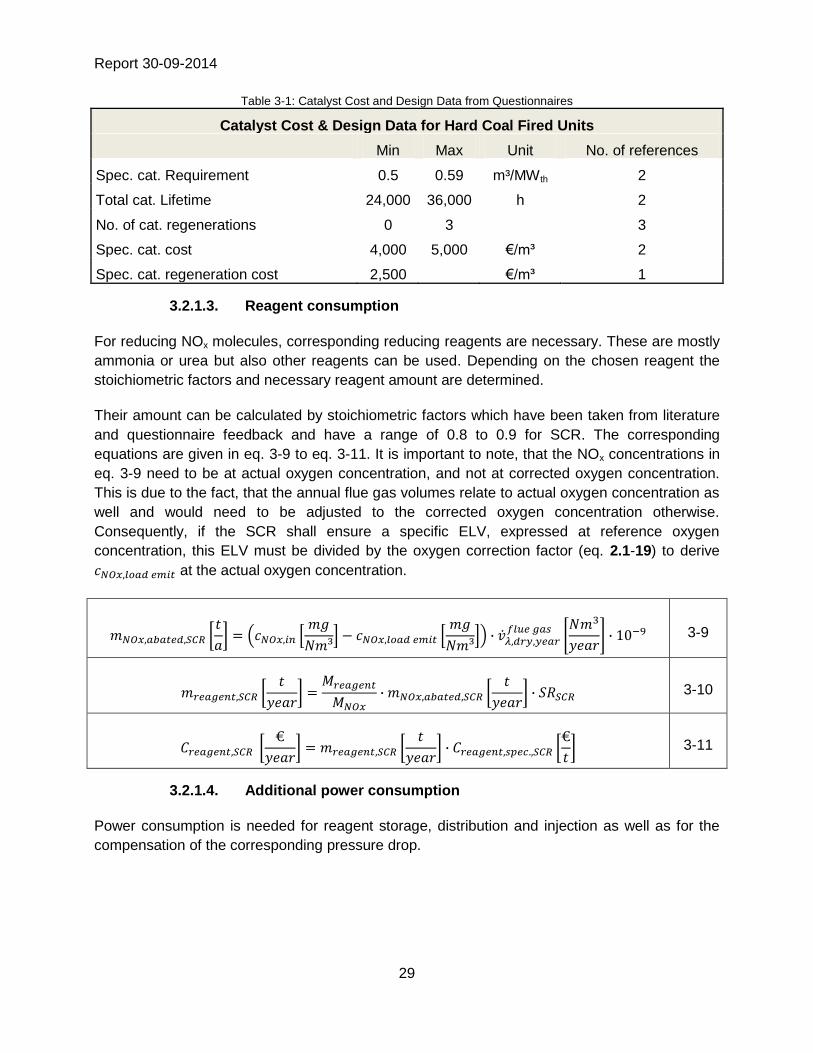
Table 3-1: Catalyst Cost and Design Data from Questionnaires
Catalyst Cost & Design Data for Hard Coal Fired Units
Min Max Unit No. of references
Spec. cat. Requirement 0.5 0.59 m³/MWth 2
Total cat. Lifetime 24,000 36,000 h 2
No. of cat. regenerations 0 3
3
Spec. cat. cost 4,000 5,000 €/m³ 2
Spec. cat. regeneration cost 2,500 €/m³ 1
3.2.1.3. Reagent consumption
For reducing NOx molecules, corresponding reducing reagents are necessary. These are mostly
ammonia or urea but also other reagents can be used. Depending on the chosen reagent the
stoichiometric factors and necessary reagent amount are determined.
Their amount can be calculated by stoichiometric factors which have been taken from literature
and questionnaire feedback and have a range of 0.8 to 0.9 for SCR. The corresponding
equations are given in eq. 3-9 to eq. 3-11. It is important to note, that the NOx concentrations in
eq. 3-9 need to be at actual oxygen concentration, and not at corrected oxygen concentration.
This is due to the fact, that the annual flue gas volumes relate to actual oxygen concentration as
well and would need to be adjusted to the corrected oxygen concentration otherwise.
Consequently, if the SCR shall ensure a specific ELV, expressed at reference oxygen
concentration, this ELV must be divided by the oxygen correction factor (eq. 2.1-19) to derive
at the actual oxygen concentration.
3-9
3-10
3-11
3.2.1.4. Additional power consumption
Power consumption is needed for reagent storage, distribution and injection as well as for the
compensation of the corresponding pressure drop.
Report 30-09-2014
30
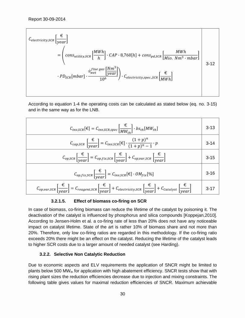
3-12
According to equation 1-4 the operating costs can be calculated as stated below (eq. no. 3-15)
and in the same way as for the LNB.
3-13
3-14
3-15
3-16
3-17
3.2.1.5. Effect of biomass co-firing on SCR
In case of biomass, co-firing biomass can reduce the lifetime of the catalyst by poisoning it. The
deactivation of the catalyst is influenced by phosphorus and silica compounds [Koppejan,2010].
According to Jensen-Holm et al. a co-firing rate of less than 20% does not have any noticeable
impact on catalyst lifetime. State of the art is rather 10% of biomass share and not more than
20%. Therefore, only low co-firing ratios are regarded in this methodology. If the co-firing ratio
exceeds 20% there might be an effect on the catalyst. Reducing the lifetime of the catalyst leads
to higher SCR costs due to a larger amount of needed catalyst (see Harding).
3.2.2. Selective Non Catalytic Reduction
Due to economic aspects and ELV requirements the application of SNCR might be limited to
plants below 500 MWth for application with high abatement efficiency. SNCR tests show that with
rising plant sizes the reduction efficiencies decrease due to injection and mixing constraints. The
following table gives values for maximal reduction efficiencies of SNCR. Maximum achievable

Report 30-09-2014
31
reduction rates decrease for larger capacities due to increasing reagent and flue gas mixing
challenges, which may lead to rising ammonia slip.
Table 3-2: Literature Data for SNCR Efficiencies
SNCR Efficiency
Maximum Achievable SNCR Reduction Rates
Plant Size Max. Reduction
< 100 MWth 60%
100 - 300 MWth 55%
300 - 500 MWth 47.5%
500 - 700 MWth 40%
> 700 MWth 35%
This table provides achieved values from SNCR retrofits. The case specific maximum
achievable NOx abatement efficiency varies from plant to plant and is in general dependent
upon the operating temperature (determined by the flue gas temperature at the point of reagent
injection and mixing), the stoichiometric reagent-to-NOx ratio, and of course, the degree of
mixing. A general interdependence between the temperature, stoichiometric ratio of ammonia,
resp. urea, and NOx to the NOx abatement efficiency can be seen in Annex E. When analysing
these diagrams, it has to be borne in mind, that ammonia ELVs (due to ammonia slip) will limit
the stoichiometric ratio in most cases and thereby inhibit abatement efficiencies of more than the
ones displayed in Table 3-3.
3.2.2.1. Reagent Consumption
The amount of reagents can be calculated by stoichiometric factors which are derived from
literature and questionnaire feedback and have a range of 1.5 to 2.0 for SNCR. It is important to
note, that the NOx concentrations in eq. 3-9 need to be at actual oxygen concentration, and not
at corrected oxygen concentration. This is due to the fact, that the annual flue gas volumes
relate to actual oxygen concentration as well and would need to be adjusted to the corrected
oxygen concentration otherwise. Consequently, if the SNCR shall ensure a specific ELV,
expressed at reference oxygen concentration, this ELV must be divided by the oxygen correction
factor (eq. 2.1-19) to derive at the actual oxygen concentration.
3-18
3-19

Report 30-09-2014
32
3-20
3.2.2.2. Pressure Drop
Contrary to the SCR the pressure drop of the SNCR is only dependent on the injection and
mixing process. Therefore, the pressure drop for calculating the needed electricity is calculated
as follows.
3-21
3.2.2.3. Additional power consumption
Power consumption is needed for reagent storage, distribution and injection as well as for the
compensation of the corresponding pressure drop.
3-22
3.2.2.4. Total costs
SNCR does not utilize catalysts. Therefore, the operating costs for SNCR only include cost for
electricity and reagent. These are calculated according to the cost functions given in chapter 1.1
and respectively to the calculation of SCR. The specific NOX abatement costs can be calculated
by dividing the total cost of capital costs and operational costs by the total NOX abated.
3-23
3-24

Report 30-09-2014
33
3-25
3-26
3-27
Report 30-09-2014
34
4. Evaluation of dust abatement techniques
4.1. Introduction
To control dust emission from Large Combustion Plant (LCP), two techniques are considered in
this report: Pulse Jet Fabric Filter and Electrostatic Precipitator (PJFF and ESP).
US EPA Air Pollution Cost Control Manual [EPA, 2002] is a reference in bottom-up approach for
cleaning process cost estimations. PJFF and ESP investment calculations developed in this
working document are based on the US EPA general approach and adapted with current data
and reference literature.
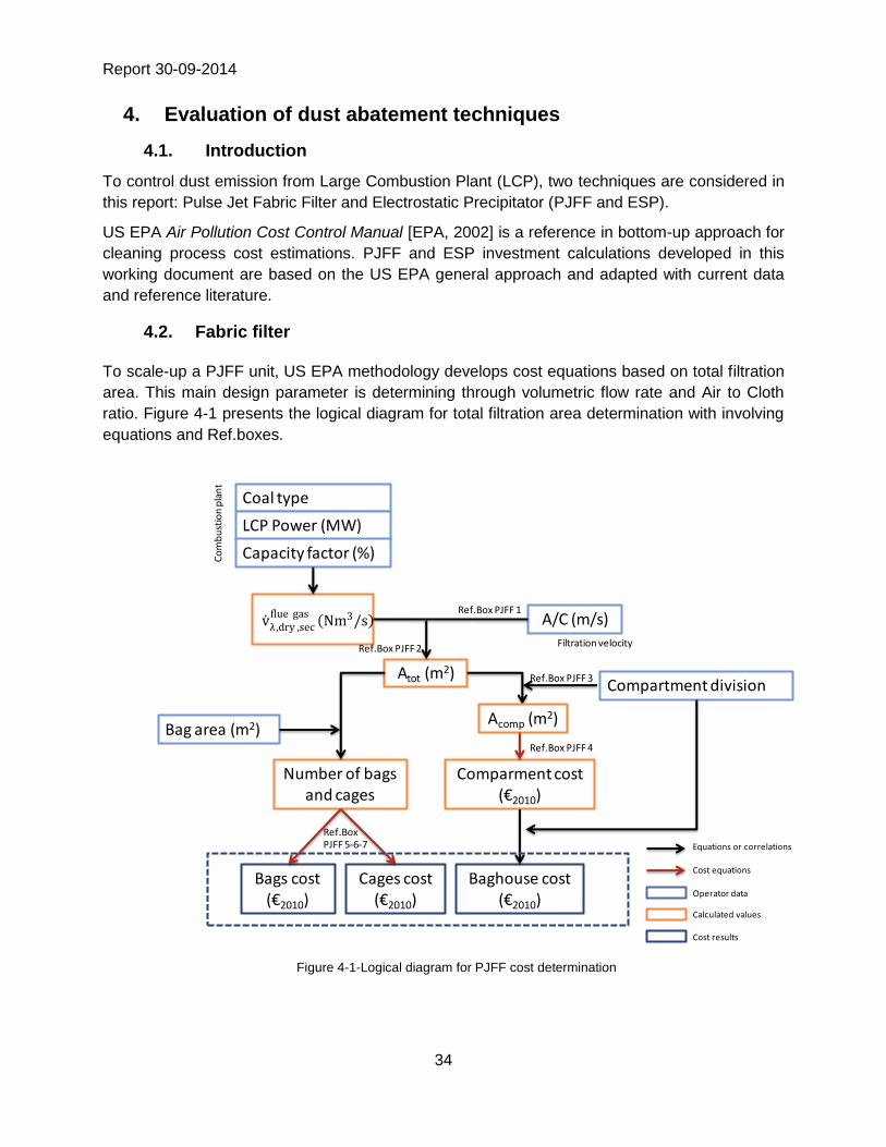
4.2. Fabric filter
To scale-up a PJFF unit, US EPA methodology develops cost equations based on total filtration
area. This main design parameter is determining through volumetric flow rate and Air to Cloth
ratio. Figure 4-1 presents the logical diagram for total filtration area determination with involving
equations and Ref.boxes.
Figure 4-1-Logical diagram for PJFF cost determination
Cages cost(€2010)
Comparment cost(€2010)
Bags cost(€2010)
Coal type
LCP Power (MW)
Capacity factor (%)
A/C (m/s)
Bag area (m2)
Atot (m2)
Number of bagsand cages
Baghouse cost(€2010)
Compartment division
Equations or correlations
Cost equations
Operator data
Calculated values
Cost results
Co
mb
ust
ion
pla
nt
Filtration velocity
Acomp (m2)
Ref.Box PJFF 1
Ref.Box PJFF 2
Ref.Box PJFF 3
Ref.Box PJFF 4
Ref.BoxPJFF 5-6-7
v λ ,dry ,secflue gas
Nm3/s
Report 30-09-2014
35
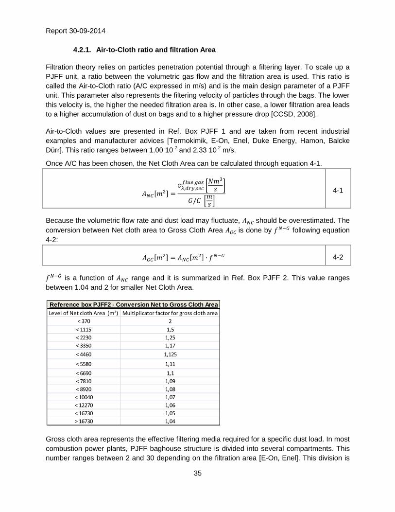
4.2.1. Air-to-Cloth ratio and filtration Area
Filtration theory relies on particles penetration potential through a filtering layer. To scale up a
PJFF unit, a ratio between the volumetric gas flow and the filtration area is used. This ratio is
called the Air-to-Cloth ratio (A/C expressed in m/s) and is the main design parameter of a PJFF
unit. This parameter also represents the filtering velocity of particles through the bags. The lower
this velocity is, the higher the needed filtration area is. In other case, a lower filtration area leads
to a higher accumulation of dust on bags and to a higher pressure drop [CCSD, 2008].
Air-to-Cloth values are presented in Ref. Box PJFF 1 and are taken from recent industrial
examples and manufacturer advices [Termokimik, E-On, Enel, Duke Energy, Hamon, Balcke
Dürr]. This ratio ranges between 1.00 10-2 and 2.33 10-2 m/s.
Once A/C has been chosen, the Net Cloth Area can be calculated through equation 4-1.
4-1
Because the volumetric flow rate and dust load may fluctuate, should be overestimated. The
conversion between Net cloth area to Gross Cloth Area is done by following equation
4-2:
4-2
is a function of range and it is summarized in Ref. Box PJFF 2. This value ranges
between 1.04 and 2 for smaller Net Cloth Area.
Gross cloth area represents the effective filtering media required for a specific dust load. In most
combustion power plants, PJFF baghouse structure is divided into several compartments. This
number ranges between 2 and 30 depending on the filtration area [E-On, Enel]. This division is
Level of Net cloth Area (m²) Multiplicator factor for gross cloth area
< 370 2
< 1115 1,5
< 2230 1,25
< 3350 1,17
< 4460 1,125
< 5580 1,11
< 6690 1,1
< 7810 1,09
< 8920 1,08
< 10040 1,07
< 12270 1,06
< 16730 1,05
> 16730 1,04
Reference box PJFF2 - Conversion Net to Gross Cloth Area
Report 30-09-2014
36
done for a better dust loading and flue gas repartition. Maintenance operation and control are
easier with subdivision. Compartment area is calculated according to and the number of
compartments (equation 4-3):
4-3
Adding extra-compartment to the baghouse structure is also a common practice in large
combustion power plant. It has several advantages:
Cleaning process for PJFF requires from time to time an off-line cleaning in order to
remove sticky and sealing dusts.
One compartment can be off-line while the process is still running.
Extra-compartments enable to treat a more variable dust charge.
Maintenance and bag replacement can be done while flue gases are still being filtered.
Extra-compartments increase to a total filtration area according to equation 4-4:
4-4
If PJFF is designed without extra-compartments then
As example, a LCP with a thermal capacity of 1,650 MWth) presents a total average filtration
area range from 40,000 to 50,000 square meters.
4.2.2. Fabric filter equipment cost
For the PJFF investment estimations, three equipment costs (
in €2010) are distinguished.
All calculations are based on the total filtration area . (see fig. 4-4)
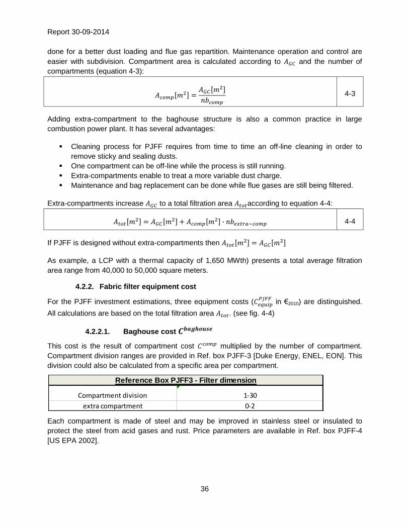
4.2.2.1. Baghouse cost
This cost is the result of compartment cost multiplied by the number of compartment.
Compartment division ranges are provided in Ref. box PJFF-3 [Duke Energy, ENEL, EON]. This
division could also be calculated from a specific area per compartment.
Each compartment is made of steel and may be improved in stainless steel or insulated to
protect the steel from acid gases and rust. Price parameters are available in Ref. box PJFF-4
[US EPA 2002].
Compartment division 1-30
extra compartment 0-2
Reference Box PJFF3 - Filter dimension

Report 30-09-2014
37
For pulse jet structure construction, two sets for cost parameters are provided [US EPA, 2002]:
For little size PJFF unit (Atot < 4,600 m²), the assembled structure is delivery on site.
In other cases, the structure is too large and must be field-assembled.
In the second condition, cost parameters are higher.
4.2.2.2. Filtering media cost
Type of filtering media defines the bag cost per square meter. The most resistant media is the
most expensive one. And naturally, the most impermeable one is also the most expensive. An
average cost per square meter is available for PE media from literature
. Ref. box PJFF-5
[US EPA, Balcke Durr, Hamon] presents media price factors referenced to PE media [US
EPA FF lesson 4] and prices per square meter of filtering media are given in Ref. box PJFF-6.
These costs
are expressed in euro per square meter and are computed with the total
filtration area to obtain
in euro (equations 4-5 and 4-6)
Baghouse type Component a (€) b (€/m2)
Basic unit 55 604 124
SS 26 789 97
Insulation 3 088 36
Basic unit 422 647 90
SS 143 808 34
Insulation 89 879 10
Pulse jet (modular)
Reference box PJFF4 - Price parameters for baghouse compartments - 2010 €
Field assembled units
PE 1
CO 1,1
PP 1,2
FG 2,5
NO 5,0
RT 6,3
P8 7,5
TF 9,4
Reference box PJFF5 - Bag cost factors for various materials
PE media price (€/m2) 5-9
Cage price (€/m2 filtering media) 16-25
Reference Box PJFF6 - Price Utilities
Report 30-09-2014
38
4-5
4-6
For coal combustion plant, typical filtering media used is PPS or Ryton. It could be improved in
P84 or with a Teflon membrane for high temperature and corrosive fumes.
4.2.2.3. Cage cost
Pulse jet cleaning needs counter-current compressed air to remove the dust cake from filter
media. In order not to deflate bags, cages are installed inside the bags. Prices per square meter
of filtering media are given in Ref. box PJFF-6 (see above).
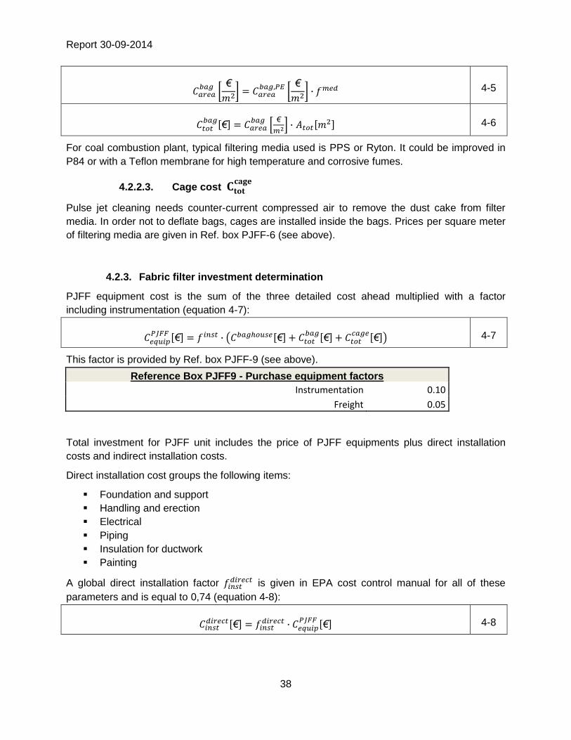
4.2.3. Fabric filter investment determination
PJFF equipment cost is the sum of the three detailed cost ahead multiplied with a factor
including instrumentation (equation 4-7):
4-7
This factor is provided by Ref. box PJFF-9 (see above).
Reference Box PJFF9 - Purchase equipment factors
Instrumentation 0.10
Freight 0.05
Total investment for PJFF unit includes the price of PJFF equipments plus direct installation
costs and indirect installation costs.
Direct installation cost groups the following items:
Foundation and support
Handling and erection
Electrical
Piping
Insulation for ductwork
Painting
A global direct installation factor is given in EPA cost control manual for all of these
parameters and is equal to 0,74 (equation 4-8):
4-8
Report 30-09-2014
39
Indirect installation costs include:
Engineering
Construction and filed expense
Contractor fees
Start-up
Performance test
Contingencies
All of these parameters result in a global indirect installation factor equal to 0.45 of
[US
EPA 2002] (equation 4-9):
4-9
Finally, total investment cost is the sum of equations 4-7, 4-8 and 4-9 (equation 4-10)
4-10
The investment cost calculated by this methodology represents the cost for a new PJFF unit. In
case of an existing plant, a retrofit factor should be applied. The value of retrofit factor ranges
between 0.3 and 0.5 [Nalbandian, 2006] and is set to 0.4 in this report.
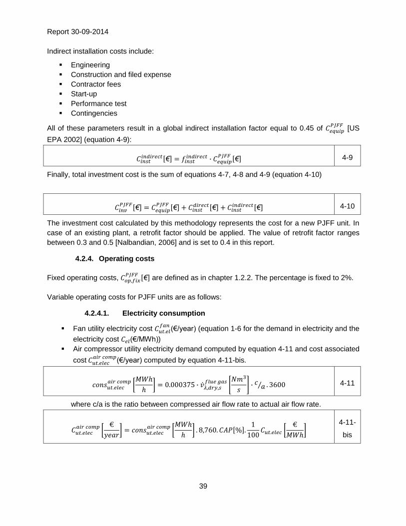
4.2.4. Operating costs
Fixed operating costs, are defined as in chapter 1.2.2. The percentage is fixed to 2%.
Variable operating costs for PJFF units are as follows:
4.2.4.1. Electricity consumption
Fan utility electricity cost
(€/year) (equation 1-6 for the demand in electricity and the
electricity cost (€/MWh))
Air compressor utility electricity demand computed by equation 4-11 and cost associated
cost
(€/year) computed by equation 4-11-bis.
4-11
where c/a is the ratio between compressed air flow rate to actual air flow rate.
4-11-
bis
Report 30-09-2014
40
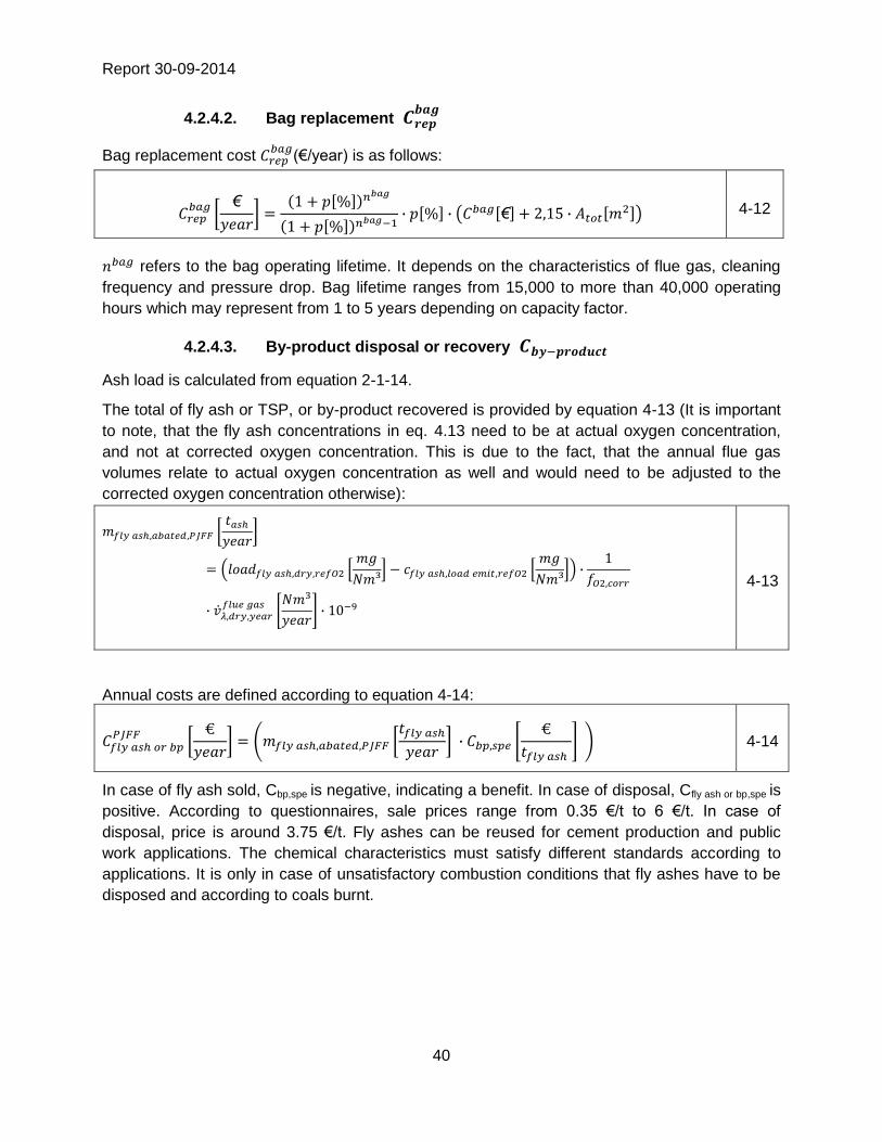
4.2.4.2. Bag replacement
Bag replacement cost
(€/year) is as follows:
4-12
refers to the bag operating lifetime. It depends on the characteristics of flue gas, cleaning
frequency and pressure drop. Bag lifetime ranges from 15,000 to more than 40,000 operating
hours which may represent from 1 to 5 years depending on capacity factor.
4.2.4.3. By-product disposal or recovery
Ash load is calculated from equation 2-1-14.
The total of fly ash or TSP, or by-product recovered is provided by equation 4-13 (It is important
to note, that the fly ash concentrations in eq. 4.13 need to be at actual oxygen concentration,
and not at corrected oxygen concentration. This is due to the fact, that the annual flue gas
volumes relate to actual oxygen concentration as well and would need to be adjusted to the
corrected oxygen concentration otherwise):
4-13
Annual costs are defined according to equation 4-14:
4-14
In case of fly ash sold, Cbp,spe is negative, indicating a benefit. In case of disposal, Cfly ash or bp,spe
is
positive. According to questionnaires, sale prices range from 0.35 €/t to 6 €/t. In case of
disposal, price is around 3.75 €/t. Fly ashes can be reused for cement production and public
work applications. The chemical characteristics must satisfy different standards according to
applications. It is only in case of unsatisfactory combustion conditions that fly ashes have to be
disposed and according to coals burnt.

Report 30-09-2014
41
4.2.5. Efficiency of PJFF
Efficiency of Pulse Jet Fabric Filters is assumed to be higher than 99.0% and may reach 99.99%
[US EPA, Hamon, CCSD]. This efficiency is not related to PJFF design but more on operation
practice.
The cleaning efficiency of FF results of the low porosity of filtering media. This permeability
decreases with the dust accumulation on bags which creates a double filtering layer. This double
layer increases the pressure drop across the bags and more fan power is required to counter
this air resistance. To control the efficiency and the pressure drop, a compromise should be
found regarding the cleaning frequency. Indeed, on the one hand if the cleaning frequency is
low, the efficiency will be improved to the detriment of pressure drop and electricity consumption.
On the other hand, a too high cleaning frequency reduces the efficiency. The bag lifetime is
indeed impacted by cleaning frequency: an increase of compressed air injection results in an
increase of maintenance and replacement operations.
To illustrate the influence of main input parameters on output parameters i.e. investment costs
and operating costs, the following table is provided:
Results on output parameters
)
Increasing input parameters
A/C ↗ ↗ ↗ ↘ ↗
Atot ↘ ↘ ↘** ↗ ↘
Fcleaning* ↘ ↘ ↘ - ↗
Table 4-1 Resulting influence of design parameters
*Fcleaning represents the cleaning frequency of filtering media. This input parameter is not developed in the
methodology because of the lack of data.
**assuming a medium porosity of filtering media
Table 4-1 presents the result of an increase of the 3 main design parameters on 5 output
parameters. One thing that has to be kept in mind that A/C and Atot evolves in opposite way.
4.3. Electro Static Precipitator
4.3.1. Investment costs
Effective Collecting Plate Area (m2) is the main design parameter to scale up an ESP unit.
Chapter 4.3.1.1 develops the approaching method to calculate the and chapter 4.3.1.2
presents the leading equations to estimate costs and investments.
4.3.1.1. Bottom up approach for value
The ESP main design parameter is the effective collecting plate area (m2). The aim of the
method used in US EPA methodology is to approach the Specific Collecting Area SCA (s/m)
which is the ratio between . and
. This method requires several input parameters:

Report 30-09-2014
42
Efficiency
Temperature
Mass mean diameter
The presence or not of Back Corona (BC)
Several factors (see Ref.box ESP 1 in excel file and table below)
Reference box ESP-1 Values for A ECP determination
Parameter Value Unit Source
Temperature (T) 380-500 [K] [CCSD 2008 ; Zevenhoven & Kilpinen]
Mass mean Diameter ( ) 3-21 [µm] [US EPA, 2002 ; Juda-Rezler, Kowalczyk, 2012]
Sneakage factor ( ) 0,07
[US EPA, 2002]
Raping reentrainment factor ( ) 0,14
[US EPA, 2002]
Most penetrating size ( ) 2 [µm] [US EPA, 2002]
Rapping puff size ( ) 5 [µm] [US EPA, 2002]
Free space permittivity (ε0) 8,845E-12 [F/m]
Loss factor ( ) 0,2002 [US EPA, 2002]
Fly ash resistivity depends on numerous parameters such as the chemical composition, the temperature, moisture content...
For simplification reasons, ESP design calculations have been developed for ash resistivity in a range adapted to its correct efficiency, between 108 and 2.1011 ohm.cm.
Temperature is required to calculate the gas viscosity and the electric field at sparking
(equations 4-15 and 4-16):
4-15
4-16
Penetration parameter (pe in %) represents the percentage of non collected dust.
4-17
Average electric field is derived from equation 4-18, taking into account the presence or not
of BC effect represented by factor .This factor equals 0.57 if no back corona occurs and 0.4
in other case.
Report 30-09-2014
43
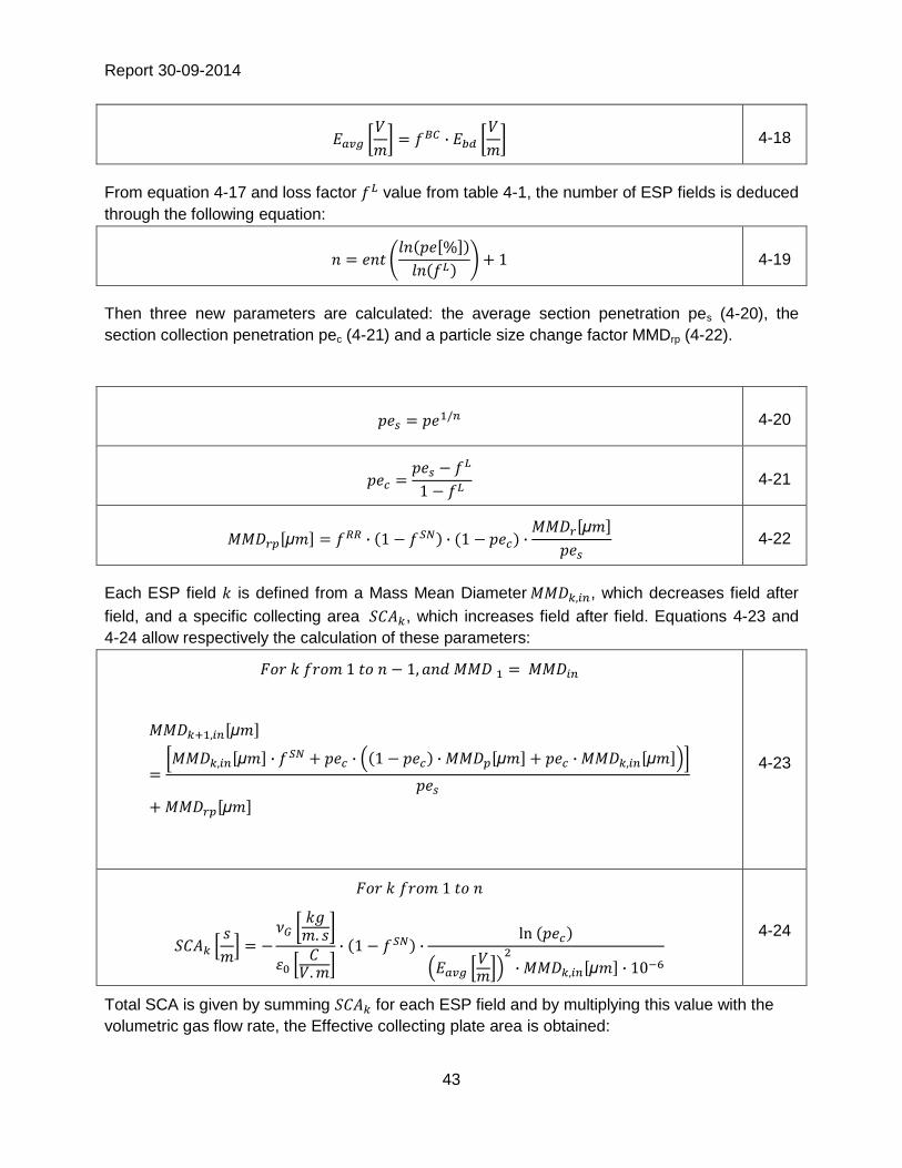
4-18
From equation 4-17 and loss factor value from table 4-1, the number of ESP fields is deduced
through the following equation:
4-19
Then three new parameters are calculated: the average section penetration pes (4-20), the
section collection penetration pec (4-21) and a particle size change factor MMDrp (4-22).
4-20
4-21
4-22
Each ESP field is defined from a Mass Mean Diameter , which decreases field after
field, and a specific collecting area , which increases field after field. Equations 4-23 and
4-24 allow respectively the calculation of these parameters:
4-23
4-24
Total SCA is given by summing for each ESP field and by multiplying this value with the
volumetric gas flow rate, the Effective collecting plate area is obtained:
Report 30-09-2014
44
4-25
4-26
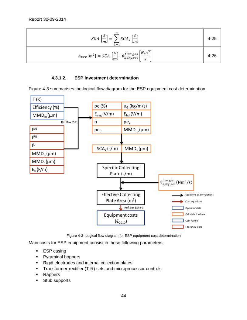
4.3.1.2. ESP investment determination
Figure 4-3 summarises the logical flow diagram for the ESP equipment cost determination.
Figure 4-3- Logical flow diagram for ESP equipment cost determination
Main costs for ESP equipment consist in these following parameters:
ESP casing
Pyramidal hoppers
Rigid electrodes and internal collection plates
Transformer-rectifier (T-R) sets and microprocessor controls
Rappers
Stub supports
fSN
MMDin (µm)
fRR
Efficiency (%)
Specific CollectingPlate (s/m)
Effective CollectingPlate Area (m²)
Equipment costs(€2010)
T (K)
MMDp (µm)
MMDr (µm)
fL
Ε0 (F/m)
pe (%)
Ebd (V/m)
υG (kg/m/s)
Eavg (V/m)
n pes
pec MMDrp (µm)
SCAk (s/m) MMDk (µm)
Ref.Box ESP1
Ref.Box ESP2-3
v λ ,dry ,secflue gas
Nm3/s
Equations or correlations
Cost equations
Operator data
Calculated values
Cost results
Literature data

Report 30-09-2014
45
US EPA develops equations for both costs, depending on effective collecting plate area.
4-27
In equation 4-27, a and b are price parameter given by Ref. box ESP-2. These parameters are
also available for “all-standard-option” installation [US EPA, lesson 4].
According to US EPA, “all-standard-option” includes:
Inlet and outlet nozzles and diffuser plates
Hopper auxiliaries/heaters, level detectors
Weather enclosure and stair access
Structural supports
Insulation
If the flue gas is corrosive, compartments have to be protected and be in stainless steel or more
resistant material. Material factors are available in ref.box ESP-3 to derive the
calculated value .
A global installation factor is given in EPA cost control manual in ref. Box ESP-5.
is given by equation 4-28:
4-28
Total investment for ESP unit includes the price of ESP equipment plus the following installation
parameters:
Foundation and support
Plate area inferior limit (m2) a b
AECP ≤ 4645 m2 3 496 0,6275
AECP > 4645 m2 549 0,8431
AECP ≤ 4645 m2 5 069 0,6276
AECP > 4645 m2 796 0,8431
Basic unit
Reference box ESP-2 Equipment cost in 2010 €
All standard option
Material Factor
Carbon Steel 1
Stainless steel 304 1,3
Stainless steel 316 1,7
Carpenter 20 CB-3 1,9
Monel-400 2,3
Nickel-200 3,2
Titanium 4,5
Reference box ESP-3 cost using various materials

Report 30-09-2014
46
Handling and erection
Electrical
Piping
Insulation for ductwork
Painting
A global direct installation factor is given in EPA cost control manual for all of these
parameters and is equal to 0,67 (equation 4-28bis):
4-28
bis
Indirect installation costs include:
Engineering
Construction and filed expense
Contractor fees
Start-up
Performance test
Contingencies
All of these parameters result in a global indirect installation factor equal to 0.57 of
[US EPA 2002] (equation 4-28 ter):
4-28
ter
Finally, total investment cost is the sum of equation 4-28, 4-28 bis and 4-28 ter (equation 4-28
four)
4-28
four
In case of an existing plant, a retrofit factor should be applied. The value of retrofit factor ranges
between 0.3 and 0.5 [Nalbandian, 2006] and is set to 0.4 in this report.

Report 30-09-2014
47
4.3.2. Operating costs
Fixed operating costs defined in chapter 1.1.2.
Operating Costs are as follows:
4.3.2.1. Electricity consumption
Fan utility electricity consumption (MWh/h) (equation 1-6)
ESP power requirement (MWh/h) (equation 4-29)
4-29
4.3.2.2. SO3 consumption
SO3 is injected in ESP in order to decrease the ash resistivity. Ash resistivity depends on the
temperature, their moisture content, their sulphur content and their chemical composition. Ash
particles can reach high resistivity values [US EPA, lesson 3]. In that case, the electric power
used to collect particles become insufficient and the ESP has to be enlarged. This phenomenon
is called the back corona. In order to avoid the back corona effect, SO3 is injected in the fumes
before the ESP [Evonik, 2011].
Due to too complex ash resistivity calculation, simple hypotheses have been developed. These hypotheses have been discussed by industrial experts [EDF 2013, HAMON2013].
In the EGTEI methodology, we assume that only coal ashes could lead to the back corona effect. Indeed, we also assume that back corona effect in case of biomass co-firing is avoided by the moisture content of biomass.
For precautionary reasons, in the EGTEI methodology, SO3 may be systematically injected to prevent coal ash high resistivity.
The SO3 consumption cost is given by the following equation:
4-30
Ref. box ESP 6 gives a range of SO3 consumption:
SO3 injection rate (kg/h) 10-80
Sulfur cost (€/t) 70
Reference Box ESP-6 SO3 conditionning
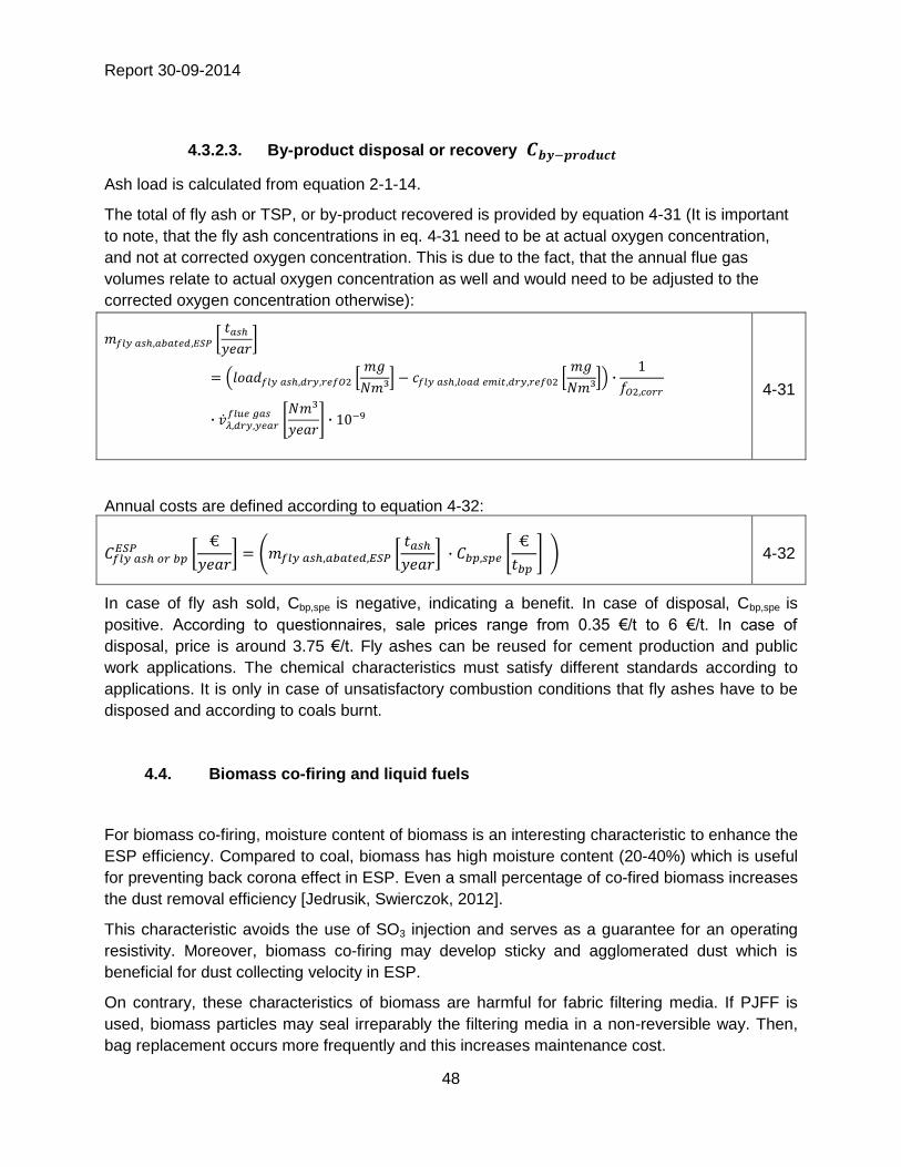
Report 30-09-2014
48
4.3.2.3. By-product disposal or recovery
Ash load is calculated from equation 2-1-14.
The total of fly ash or TSP, or by-product recovered is provided by equation 4-31 (It is important
to note, that the fly ash concentrations in eq. 4-31 need to be at actual oxygen concentration,
and not at corrected oxygen concentration. This is due to the fact, that the annual flue gas
volumes relate to actual oxygen concentration as well and would need to be adjusted to the
corrected oxygen concentration otherwise):
4-31
Annual costs are defined according to equation 4-32:
4-32
In case of fly ash sold, Cbp,spe is negative, indicating a benefit. In case of disposal, Cbp,spe
is
positive. According to questionnaires, sale prices range from 0.35 €/t to 6 €/t. In case of
disposal, price is around 3.75 €/t. Fly ashes can be reused for cement production and public
work applications. The chemical characteristics must satisfy different standards according to
applications. It is only in case of unsatisfactory combustion conditions that fly ashes have to be
disposed and according to coals burnt.
4.4. Biomass co-firing and liquid fuels
For biomass co-firing, moisture content of biomass is an interesting characteristic to enhance the
ESP efficiency. Compared to coal, biomass has high moisture content (20-40%) which is useful
for preventing back corona effect in ESP. Even a small percentage of co-fired biomass increases
the dust removal efficiency [Jedrusik, Swierczok, 2012].
This characteristic avoids the use of SO3 injection and serves as a guarantee for an operating
resistivity. Moreover, biomass co-firing may develop sticky and agglomerated dust which is
beneficial for dust collecting velocity in ESP.
On contrary, these characteristics of biomass are harmful for fabric filtering media. If PJFF is
used, biomass particles may seal irreparably the filtering media in a non-reversible way. Then,
bag replacement occurs more frequently and this increases maintenance cost.

Report 30-09-2014
49
For the same reason, heavy liquid fuel requires an ESP to eliminate combustion particles.
Unburned combustion particles may plug the filtering media as well as biomass particles
[Hamon, 2013].

Report 30-09-2014
50
5. Evaluation of SO2 abatement techniques
Three abatement techniques are considered:
Wet flue gas desulphurisation (FGD) with limestone forced oxidation (LSFO FGD). This
technique is frequently used in coal combustion plants. According to [Nalbandian 2006], it
represents 89 % of the market share for these coal combustion plants. There is rare
information for plants using liquid fuels. The LFSO FGD enables to produce commercial
grade gypsum which can be used for plaster production, cement production as well as
other applications if technical specifications are achieved (however the market is saturated
and the opportunities of valorisation decrease according to information provided). LSFO
FGD can be used theoretically for plants of any size but is generally used for the largest
ones, due to economic reasons [Nalbandian 2006]. LSFO FGD can be installed for coals
of all sulphur level, including low sulphur coals (less than 1% S) but are typically used for
coals with medium and high sulphur content (> 2% S) [Sargent 2007]. Efficiency can reach
range between 85 and 98% [EU Commission 2006a]. 99% is also provided [Sargent
2007], however sulphur level lower than 0.017 kg SO2/GJ is a practical outlet limitation
with the lowest sulphur content coals (about 50 mg SO2/Nm3, considering a coal average
LHV of 29 GJ/t coal).
Lime spray dryer (LSD) FGD. This technique most often employs lime in a semi-dry form.
According to [Nalbandian 2006], it represents 8% of the market share for plants using coal.
No information is available for plants using liquid fuels. Polluted gas stream is brought into
contact with lime in a spray dryer. A fabric filter is used just after, to remove dust and
calcium sulphates and sulphites formed during desulphurisation. Lime spray dryers can be
used for plants theoretically of any size. However, they are mainly observed for plants
lower than 250 MWe capacity (and at maximum 350 MWe) [Nalbandian 2006]. By-
products have fewer uses than those of LSFO FGD, due to their properties (mixture of fly
ashes and by-products).
LSD FGD is used for low and medium sulphur coal (< 1.5% S) [Nalbandian 2006].
Efficiency ranges between 70 to 90 % [EU Commission, 2006a]. 95% is also provided by
Sargent 2007] depending on the ratio Ca/S.
Dry FGD. They are several arrangements for dry FGD [EU Commission, 2006a]. The duct
sorbent injection FGD is considered for cost estimation (DSI FGD). Dry hydrated lime
(Ca(OH)2) or quick lime (CaO) can be used. Due to high amount of un-reacted sorbent,
recycling of products must be often operated several times. The specific surface of lime is
crucial for the efficiency of the process and lime prices depend on this characteristic.
According to [EU commission, 2006a], the existing ESP can be kept in operation in case of
retrofit (It is explained, that the way an ESP is able to collect 100 times more product and
fly ash than at a single throughput to a duct injection process, is not well understood). In
the cost determination developed, the use of a fabric filter is considered. Dry FGD
efficiency ranges from 50 to 80 % [EU Commission, 2006a].
Other reagents are also used such as sodium bicarbonate (NaHCO3) and performances
can be different. In this document, cost estimation is only developed for use of lime. Use of
sodium bicarbonate must be included in the next months (before end 2014).
Report 30-09-2014
51
5.1. LSFO FGD
5.1.1. Investment costs
Annex D presents capital costs available in the literature and collected from the questionnaires
received from plant operators in the EU. The cost function developed by US EPA from a study
carried by Sargent and Lundy (Sargent 2010b), has been selected to represent the evolution of
investment according to the size of the combustion plant and its characteristics.
The US EPA cost function has been adapted to accept units of this report (international system
of units) and express costs in Euro.
The investment includes three groups of cost:
1 - The unit cost itself:
includes all equipment, installation, buildings, foundations, electrical, minor waste water
treatment and take into account the retrofit difficulty. The cost function to derive includes
different modules:
absorber unit cost ,
reagent preparation unit cost ,
waste handling unit cost ,
base balance of plan costs including: ID or booster fans, new wet chimney, piping,
ductwork, minor waste water treatment, etc. .
which is the sum of the four components, is the total unit cost.
The US EPA model assumes a wet chimney and no gas/gas heater after the SO2 absorber.
According to [Nalbandian 2006] and confirmed by the EGTEI LCP working group, this is
presently a common practice. After the wet absorber, the chimney exit temperature can be as
low as 50 °C. The use of a wet chimney instead of a dry chimney avoids installation of a gas/gas
heater. The main advantages of omitting the gas/gas heater are provided by [Nalbandian 2006]:
Cost,
Removal of a maintenance intensive piece of equipment,
Lower additional auxiliary power consumption.
A wet chimney is however expensive as it must be corrosion resistant (and has to be built in
alloy, alloy carbon steel on contrary to a dry chimney constructed in traditional carbon steel
[Sargent 2007]). With a wet chimney, the risk of a visible plume is higher than with a dry
chimney.
2 – Additional indirect cost for:
Engineering and construction management,
Labour cost for construction (labour adjustments for 6 x 10 hour shift premium, per diem),
Contractor profit and fees.
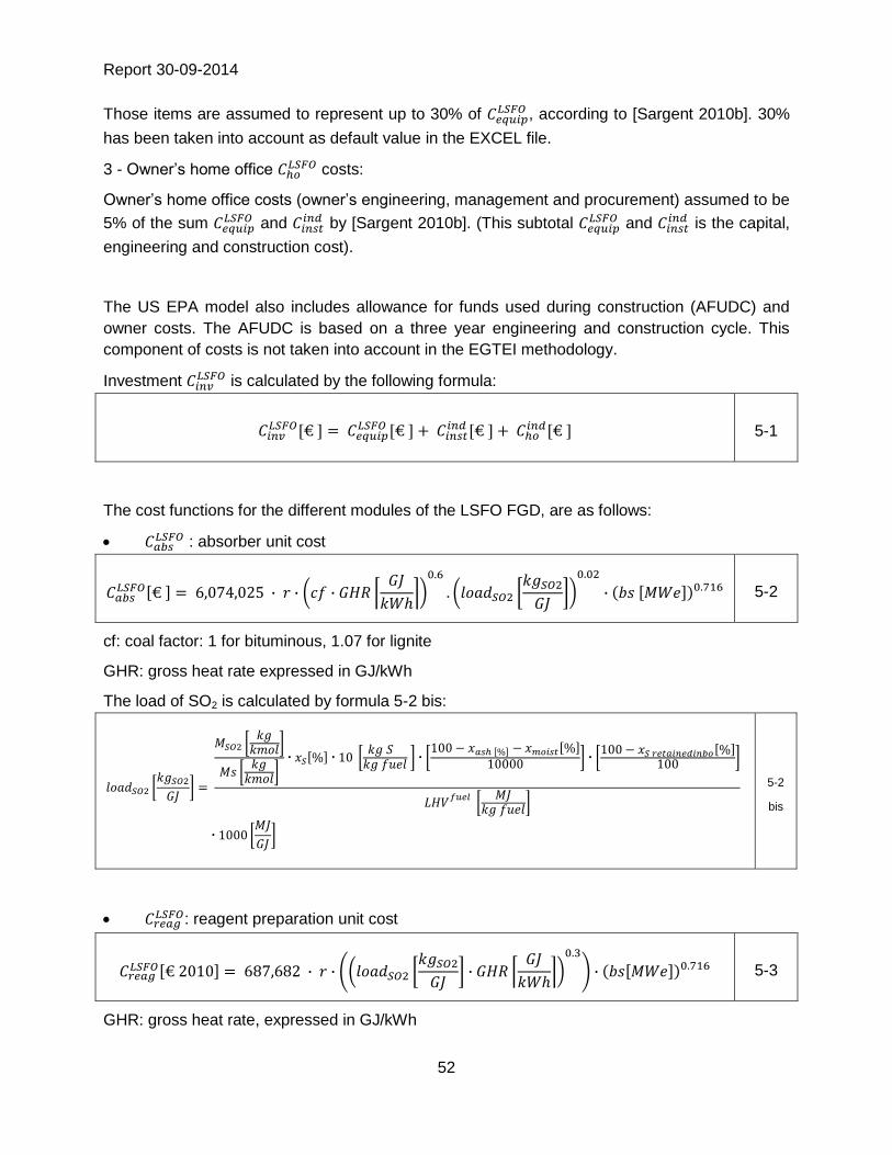
Report 30-09-2014
52
Those items are assumed to represent up to 30% of , according to [Sargent 2010b]. 30%
has been taken into account as default value in the EXCEL file.
3 - Owner’s home office costs:
Owner’s home office costs (owner’s engineering, management and procurement) assumed to be
5% of the sum and
by [Sargent 2010b]. (This subtotal and
is the capital,
engineering and construction cost).
The US EPA model also includes allowance for funds used during construction (AFUDC) and
owner costs. The AFUDC is based on a three year engineering and construction cycle. This
component of costs is not taken into account in the EGTEI methodology.
Investment is calculated by the following formula:
5-1
The cost functions for the different modules of the LSFO FGD, are as follows:
: absorber unit cost
5-2
cf: coal factor: 1 for bituminous, 1.07 for lignite
GHR: gross heat rate expressed in GJ/kWh
The load of SO2 is calculated by formula 5-2 bis:
5-2
bis
: reagent preparation unit cost
5-3
GHR: gross heat rate, expressed in GJ/kWh
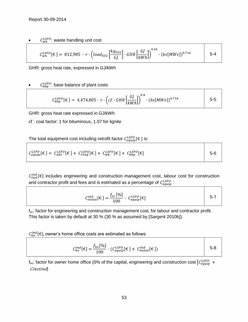
Report 30-09-2014
53
: waste handling unit cost
5-4
GHR: gross heat rate, expressed in GJ/kWh
: base balance of plant costs
5-5
GHR: gross heat rate expressed in GJ/kWh
cf : coal factor: 1 for bituminous, 1.07 for lignite
The total equipment cost including retrofit factor is:
5-6
includes engineering and construction management cost, labour cost for construction
and contractor profit and fees and is estimated as a percentage of :
5-7
fec: factor for engineering and construction management cost, for labour and contractor profit.
This factor is taken by default at 30 % (30 % as assumed by [Sargent 2010b]).
owner’s home office costs are estimated as follows:
5-8
fho: factor for owner home office (5% of the capital, engineering and construction cost
)

Report 30-09-2014
54
5.1.2. Operating costs
Annual operating costs (Cop) include fixed operating and maintenance costs (Cop,fix) and variable
operating costs (Cop,var).
Fixed operating costs
As presented in chapter 1.1.2, fixed operating costs are calculated as a percentage of the unit
cost . Based on [US EPA 2010], the factor OMfix in % of the investment is a function of
the size of the plant. From data presented [US EPA 2010], the following function can be derived:
5-9
Variable operating costs
For this technique, variable operating costs include auxiliary power, limestone consumption cost,
and waste handling cost. Make-up water cost [Sargent 2010b] has been neglected, as quite low
compared to other cost items.
5.1.2.1. Auxiliary electricity
The auxiliary power penalty ranges from 1 to 2% of the plant capacity according to [Sargent
2010b] and experts of the EGTEI LCP working group. Higher power penalty can be observed
when a gas/gas heater is present [Nalbandian 2006, EGTEI experts].
The penalty has been derived from data of power penalty provided by [US EPA 2010] according
to the heat rate (electricity penalty of 1.5% for a gross heat rate of 0.0095 GJ/kWh, 1.67% for a
heat rate of 0.0106 GJ/kWh, 1.84% for a heat rate of 0.0116 GJ/kWh). A function can be derived
in which is used.
Equation 5-10 provides annual electricity consumption cost for LSFO FGD.
5-10
CAP: capacity factor in % (equation 2.1-5)
Celec,spe: specific cost of electricity in €/MWh
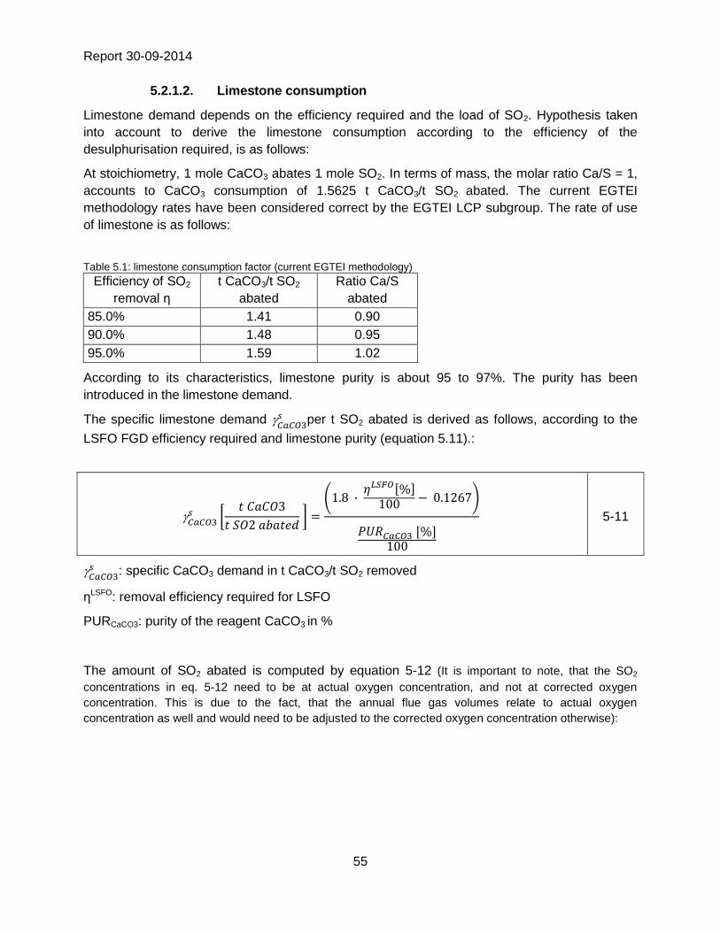
Report 30-09-2014
55
5.2.1.2. Limestone consumption
Limestone demand depends on the efficiency required and the load of SO2. Hypothesis taken
into account to derive the limestone consumption according to the efficiency of the
desulphurisation required, is as follows:
At stoichiometry, 1 mole CaCO3 abates 1 mole SO2. In terms of mass, the molar ratio Ca/S = 1,
accounts to CaCO3 consumption of 1.5625 t CaCO3/t SO2 abated. The current EGTEI
methodology rates have been considered correct by the EGTEI LCP subgroup. The rate of use
of limestone is as follows:
Table 5.1: limestone consumption factor (current EGTEI methodology)
Efficiency of SO2
removal η
t CaCO3/t SO2
abated
Ratio Ca/S
abated
85.0% 1.41 0.90
90.0% 1.48 0.95
95.0% 1.59 1.02
According to its characteristics, limestone purity is about 95 to 97%. The purity has been
introduced in the limestone demand.
The specific limestone demand per t SO2 abated is derived as follows, according to the
LSFO FGD efficiency required and limestone purity (equation 5.11).:
5-11
: specific CaCO3 demand in t CaCO3/t SO2 removed
ηLSFO: removal efficiency required for LSFO
PURCaCO3: purity of the reagent CaCO3 in %
The amount of SO2 abated is computed by equation 5-12 (It is important to note, that the SO2
concentrations in eq. 5-12 need to be at actual oxygen concentration, and not at corrected oxygen
concentration. This is due to the fact, that the annual flue gas volumes relate to actual oxygen
concentration as well and would need to be adjusted to the corrected oxygen concentration otherwise):

Report 30-09-2014
56
5-12
Equation 5-12 bis can also be used:
5-12
bis
Cost of limestone consumption is provided by equation 5-13:
5-13
CaCO3 prices depend on quantity bought and quality. From questionnaires, prices range from:
11 to 16 €/t CaCO3 in a 2465 MWth plant and 32 to 36 €/t CaCO3 in a 630 MWth plant and 40 €/t
CaCO3 in another 630 MWth plant for similar CaCO3 purity (94 % to 96 %)
5.2.1.3. By-product, disposal or recovery
In ideal situation, gypsum can be produced and sold. Commercial grade gypsum can be used in
wallboard, cement or plaster manufacturing, also soil conditioner. Special specifications have to
be observed such as chlorine content, purity, colour... [Sargent 2007]. Often, different sources of
coals can be envisaged in plants. Some coals do not enable to be in the specifications.
Presently, sale price of gypsum produced is very low and operators do not expect higher costs
(EGTEI LCP expert group). This is confirmed by [Nalbandian 2006] who also explains that sale
prices can be negative when transport costs are included.
If not sold, by-products have to be disposed in correct conditions.
According to oxidation efficiency, CaSO3.½H2O and/or CaSO4,2H2O are produced. CaSO4,2H2O
is a saleable product. It is assumed a by-product with a humidity of 10 % [EU Commission,
2006a] (This explains the factor 1.91 in equation 5.14).
: specific by-product production in ton by-product (bp)/ton SO2 removed.

Report 30-09-2014
57
5-14
Cost of waste disposal or gypsum sold is given by equation 5-15:
5-15
In case gypsum is sold, Cbp,spe is negative, indicating a benefit. In case of disposal, Cbp,spe is
positive. Price of sold gypsum can be low due to saturation of the market. Questionnaires
provide a range from 0.15 to 2 €/t by-product sold. When by-products are disposed, disposal
prices depend on the waste disposal treatment. Landfill or other treatments such as incineration
can be used. By-product disposal prices range from 0.33 to 89 €/t by-product, according to the
information obtained.
5.1.3. Adaptation of costs for installations consuming heavy fuel oil
As carried out in the current EGTEI methodology, the investment function derived for coals is
adapted for liquid fuels according to the relative flue gas volume, considering 1 for hard coal.
The average flue gas volume for coal at 6% O2 is 358 Nm3/MJ.
The average flue gas volume for heavy fuel oil at 3% O2 is 285 Nm3/MJ.
An average factor of 0.8 can be derived from those data. The investment functions presented
above for coal are adapted with this factor, as follows.
The cost functions for the different modules of the LSFO FGD for heavy fuel oils, are as follows:
: absorber unit cost
5-16
: reagent preparation unit cost
5-17

Report 30-09-2014
58
: waste handling unit cost
5-18
: base balance of plan costs
5-19
The total equipment cost including retrofit factor is provided by equation 5-6.
Other equations for total investment and operating costs do not change.
5.2. Lime spray dryer FGD (LSD FGD)
In lime spray dryer, either hydrated lime (Ca(OH)2) or quicklime (CaO) can be used. Quicklime is
more often used for economical reasons [Sargent 2007]. Lime is slaked to produce a lime milk.
Lime milk is atomised to a cloud of fine droplets in the spray dry absorber. Water is evaporated
by the heat of the flue gas [EU Commission, 2006a]. Wastes are dry because all the water is
evaporated. The residue obtained is a mixture of calcium sulphite, calcium sulphate and fly ash.
The presence of fly ash depends on the fact a deduster is maintained before the absorber (in
case of retrofit indeed, if the plant is equipped with an ESP, it can be maintained). By-products
obtained are not attractive commercially [EU Commission, 2006a].
5.2.1. Investment costs
The cost functions derived assume the use of ball mill slaker [EPA 2010]. It is unclear in this
reference, if the fabric filter is included or not in the investment function. It is assumed to be
included.
Investment is calculated by the following formula:
5-20
The cost functions for the different modules of the LSD FGD, are as follows [Sargent 2010c]:
: absorber unit cost

Report 30-09-2014
59
5-21
cf: coal factor: 1 for bituminous, 1.07 for lignite
GHR: gross heat rate expressed in GJ/kWh
loadSO2: load of SO2 expressed in kgSO2/GJ (calculated by formula 5-2 bis)
: reagent preparation and waste handling unit cost
5-22
GHR: gross heat rate expressed in GJ/kWh
loadSO2: load of SO2 expressed in kgSO2/GJ
: base balance of plan costs
5-23
GHR: gross heat rate expressed in GJ/kWh
cf : coal factor: 1 for bituminous, 1.07 for lignite
The total equipment cost including retrofit factor is:
5-24
includes engineering and construction management cost, labour cost for construction
and contractor profit and fees and is estimated as a percentage of .
5-25
fec: factor for engineering and construction management cost, for labour and contractor profit.
This factor is taken by default at 30 % (30 % as assumed by [Sargent 2010c]).

Report 30-09-2014
60
owner’s home office costs are estimated as follows:
5-26
fho : factor for owner home office (5% of the capital, engineering and construction cost
)
5.2.2. Operating costs
Annual operating costs (Cop) include fixed operating and maintenance costs (Cop,fix) and variable
operating costs (Cop,var).
Fixed operating costs
As presented in chapter 1.1.2, fixed operating costs are calculated as a percentage of the unit
cost . Based on [EPA 2010], the factor OMfix in % of the investment is a function of the
size of the plant. From data presented, the following function can be derived:
5-27
Variable operating costs
For LSD FGD, variable operating costs include auxiliary power, lime consumption cost, waste
disposal cost.
5.2.2.1. Auxiliary electricity
The auxiliary power penalty ranges from 1 to 2% of the plant capacity according to [Sargent
2010c]. Higher power penalty can be observed when a gas/gas heater is used [Nalbandian
2006, EGTEI experts].
The penalty has been derived from data of power penalty provided by [US EPA 2010] according
to the heat rate (electricity penalty of 1.2% for a heat rate of 0.0095 GJ/kWh, 1.33% for a heat
rate of 0.0106 GJ/kWh, 1.47% for a heat rate of 0.0116 GJ/kWh). A function can be derived in
which is used.
Equation 5-28 provides annual electricity consumption cost for LSD FGD.
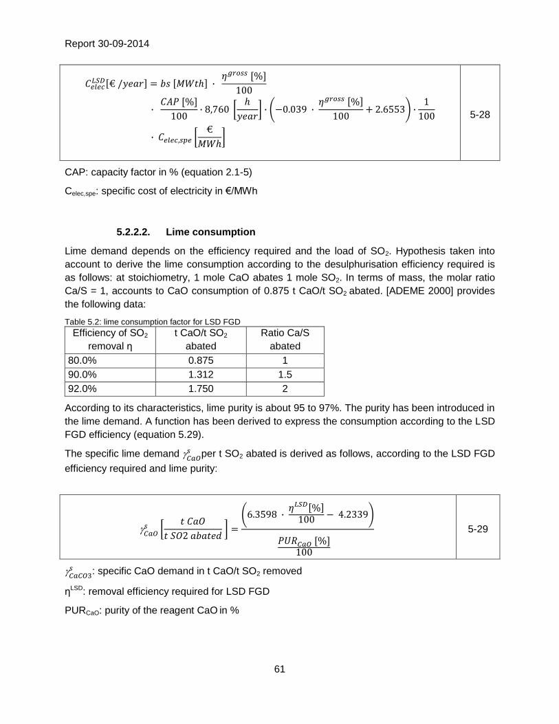
Report 30-09-2014
61
5-28
CAP: capacity factor in % (equation 2.1-5)
Celec,spe: specific cost of electricity in €/MWh
5.2.2.2. Lime consumption
Lime demand depends on the efficiency required and the load of SO2. Hypothesis taken into
account to derive the lime consumption according to the desulphurisation efficiency required is
as follows: at stoichiometry, 1 mole CaO abates 1 mole SO2. In terms of mass, the molar ratio
Ca/S = 1, accounts to CaO consumption of 0.875 t CaO/t SO2 abated. [ADEME 2000] provides
the following data:
Table 5.2: lime consumption factor for LSD FGD
Efficiency of SO2
removal η
t CaO/t SO2
abated
Ratio Ca/S
abated
80.0% 0.875 1
90.0% 1.312 1.5
92.0% 1.750 2
According to its characteristics, lime purity is about 95 to 97%. The purity has been introduced in
the lime demand. A function has been derived to express the consumption according to the LSD
FGD efficiency (equation 5.29).
The specific lime demand per t SO2 abated is derived as follows, according to the LSD FGD
efficiency required and lime purity:
5-29
: specific CaO demand in t CaO/t SO2 removed
ηLSD: removal efficiency required for LSD FGD
PURCaO: purity of the reagent CaO in %

Report 30-09-2014
62
The amount of SO2 abated is computed by equation 5-30 (It is important to note, that the SO2
concentrations in eq. 4-30 need to be at actual oxygen concentration, and not at corrected oxygen
concentration. This is due to the fact, that the annual flue gas volumes relate to actual oxygen
concentration as well and would need to be adjusted to the corrected oxygen concentration otherwise):
5-30
Cost of lime consumption is provided by equation 5-31:
5-31
CaO price is about 5 times price of limestone. Prices range from 80 to 150 €/t CaO according to
its specific surface.
5.2.2.3. By-product, disposal or recovery
According to [Sargent 2007] by products can be used for aggregate and block manufacture or
disposed. If not sold, by-products have to be disposed in correct conditions.
According to oxidation efficiency, CaSO3 and/or CaSO4, ½H2O are produced. If the LSD FGD is
installed in an existing plant, the existing ESP can be maintained and fly ashes can be
eliminated. In new plants, the presence of deduster before the absorber is not systematic. The
production of 50/50 CaSO3 and CaSO4.½H2O is assumed to calculate the by-product production
(This explains the factor 2.366 in equation 5.32).
: specific by-product production in ton by-product (bp)/ton SO2 removed.
5-32
Cost of waste disposal or gypsum sold is given by equation 5-33:
5-33
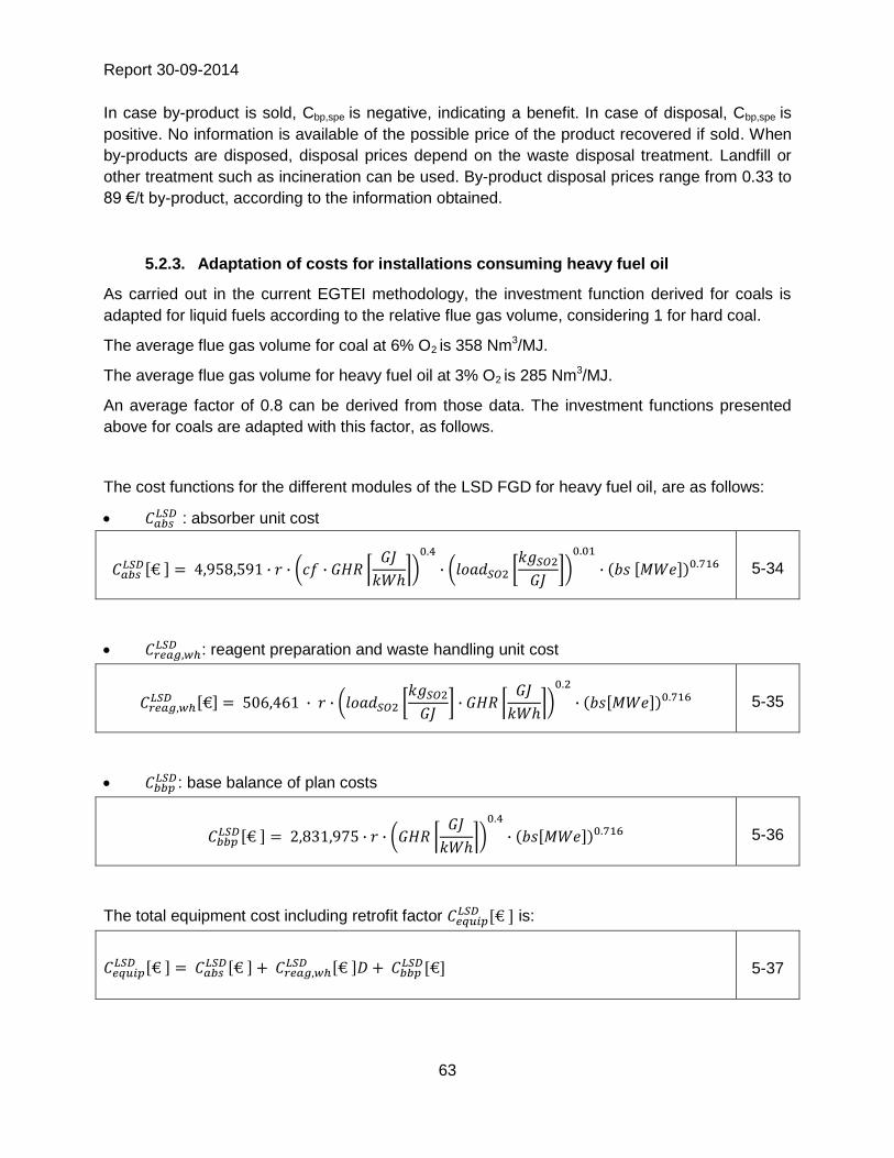
Report 30-09-2014
63
In case by-product is sold, Cbp,spe is negative, indicating a benefit. In case of disposal, Cbp,spe is
positive. No information is available of the possible price of the product recovered if sold. When
by-products are disposed, disposal prices depend on the waste disposal treatment. Landfill or
other treatment such as incineration can be used. By-product disposal prices range from 0.33 to
89 €/t by-product, according to the information obtained.
5.2.3. Adaptation of costs for installations consuming heavy fuel oil
As carried out in the current EGTEI methodology, the investment function derived for coals is
adapted for liquid fuels according to the relative flue gas volume, considering 1 for hard coal.
The average flue gas volume for coal at 6% O2 is 358 Nm3/MJ.
The average flue gas volume for heavy fuel oil at 3% O2 is 285 Nm3/MJ.
An average factor of 0.8 can be derived from those data. The investment functions presented
above for coals are adapted with this factor, as follows.
The cost functions for the different modules of the LSD FGD for heavy fuel oil, are as follows:
: absorber unit cost
5-34
: reagent preparation and waste handling unit cost
5-35
: base balance of plan costs
5-36
The total equipment cost including retrofit factor is:
5-37

Report 30-09-2014
64
includes engineering and construction management cost, labour cost for construction
and contractor profit and fees and is estimated as a percentage of .
The total equipment cost including retrofit factor is provided by equation 5-6.
Other equations for total investment and operating costs do not change.

Report 30-09-2014
65
5.3. Dry FGD
The duct sorbent injection (DSI) FGD is considered for cost estimation. Dry hydrated lime
(Ca(OH)2) or quick lime (CaO) can be used. Other reagents are also used such as sodium
bicarbonate. The use of CaO is presented hare after. Use of sodium bicarbonate will be
presented in the next update of this document and EXCEL tool.
Due to high amount of un-reacted sorbent, recycling of products must be operated several times.
The specific surface of lime is crucial for the efficiency of the process and lime prices depend on
this characteristic.
According to [EU commission, 2006a], the existing ESP can be kept in operation in case of
retrofit (It is explained that the way an ESP is able to collect 100 times more product and fly ash
than at a single throughput to a duct injection process, is not well understood).
The estimation of costs is carried out taking into account lime as reagent and assuming the
presence of a new fabric filter after the existing ESP in case of retrofit. The FF mainly eliminates
residual fly ashes and desulphurisation products. This is the technical solution proposed by most
manufacturers of dry desulphurisation techniques [Coal WG, 2013] for existing plants. The
residence time in the fabric filter is enlarged to facilitate the desulphurisation. The air to cloth
ratio of the FF has to be reduced consequently.
Efficiency ranges from 50 to 80% [EU commission, 2006a].
5.3.1. Investment costs
The duct sorbent injection FGD is less documented than wet desulphurisation techniques.
Information has been provided by experts from a French working group of the chemical industry
[Coal WG, 2013].
The main investment item is for the FF which has to be larger to enable finalisation of
desulphurisation. In case of retrofit, the existing ESP can be maintained. The FF eliminates
desulphurisation products and a small fraction of remaining fly ashes when the ESP is present.
From data provided by experts [Coal WG, 2013], additional costs for lime injection in the ducts
and lime preparation could be estimated to 30 % of the FF investment.
Lime demand depends on the deSOx efficiency required, the temperature and the load of SO2.
Hypothesis taken into account to derive the lime consumption according to the efficiency of the
desulphurisation required are as follows:
At stoichiometry, 1 mole CaO abates 1 mole SO2. In terms of mass, the molar ratio Ca/S = 1,
accounts to CaO consumption of 0.875 t CaO/t SO2 abated. [ADEME 2000] provides the
following data:
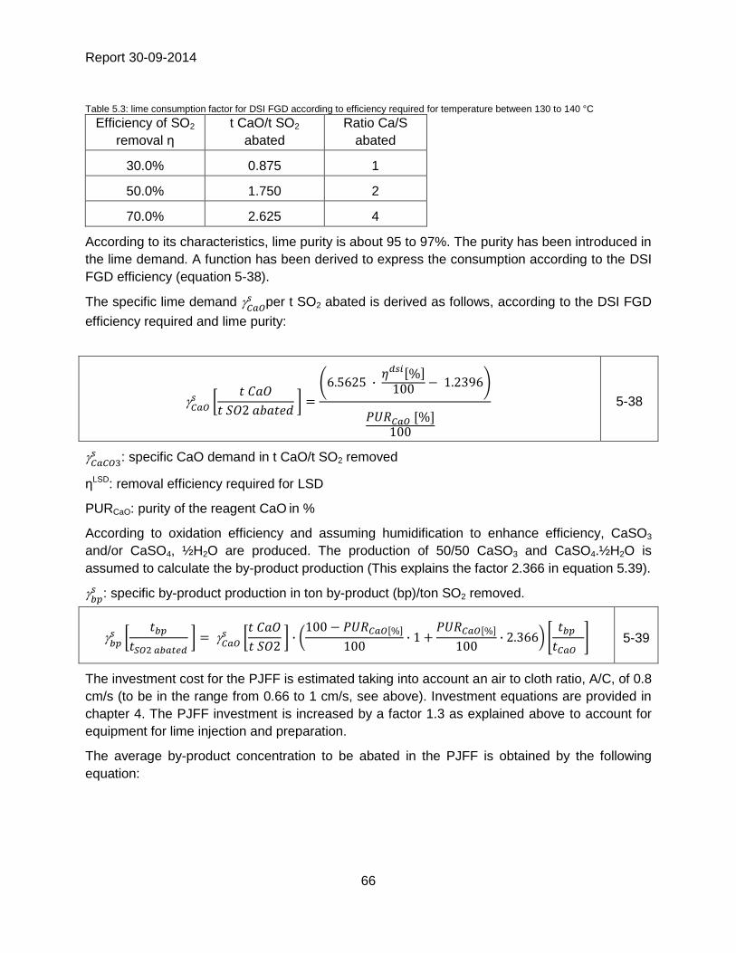
Report 30-09-2014
66
Table 5.3: lime consumption factor for DSI FGD according to efficiency required for temperature between 130 to 140 °C
Efficiency of SO2
removal η
t CaO/t SO2
abated
Ratio Ca/S
abated
30.0% 0.875 1
50.0% 1.750 2
70.0% 2.625 4
According to its characteristics, lime purity is about 95 to 97%. The purity has been introduced in
the lime demand. A function has been derived to express the consumption according to the DSI
FGD efficiency (equation 5-38).
The specific lime demand per t SO2 abated is derived as follows, according to the DSI FGD
efficiency required and lime purity:
5-38
: specific CaO demand in t CaO/t SO2 removed
ηLSD: removal efficiency required for LSD
PURCaO: purity of the reagent CaO in %
According to oxidation efficiency and assuming humidification to enhance efficiency, CaSO3
and/or CaSO4, ½H2O are produced. The production of 50/50 CaSO3 and CaSO4.½H2O is
assumed to calculate the by-product production (This explains the factor 2.366 in equation 5.39).
: specific by-product production in ton by-product (bp)/ton SO2 removed.
5-39
The investment cost for the PJFF is estimated taking into account an air to cloth ratio, A/C, of 0.8
cm/s (to be in the range from 0.66 to 1 cm/s, see above). Investment equations are provided in
chapter 4. The PJFF investment is increased by a factor 1.3 as explained above to account for
equipment for lime injection and preparation.
The average by-product concentration to be abated in the PJFF is obtained by the following
equation:
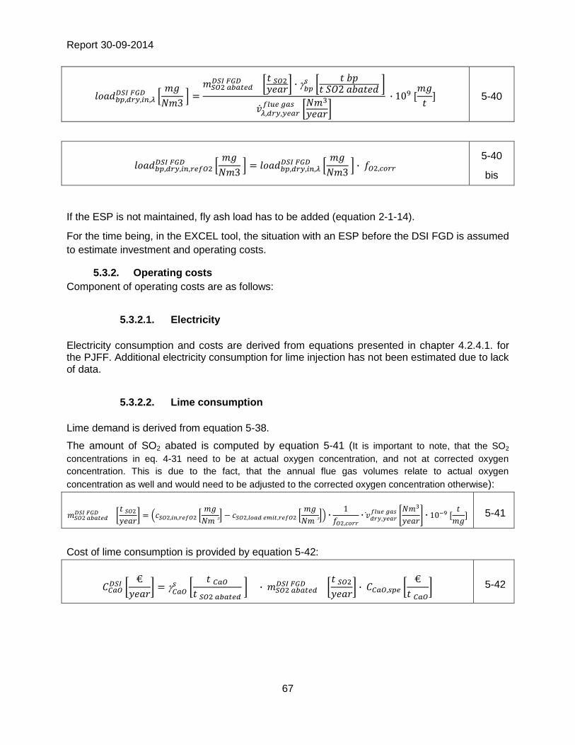
Report 30-09-2014
67
5-40
5-40
bis
If the ESP is not maintained, fly ash load has to be added (equation 2-1-14).
For the time being, in the EXCEL tool, the situation with an ESP before the DSI FGD is assumed
to estimate investment and operating costs.
5.3.2. Operating costs
Component of operating costs are as follows:
5.3.2.1. Electricity
Electricity consumption and costs are derived from equations presented in chapter 4.2.4.1. for the PJFF. Additional electricity consumption for lime injection has not been estimated due to lack of data.
5.3.2.2. Lime consumption
Lime demand is derived from equation 5-38.
The amount of SO2 abated is computed by equation 5-41 (It is important to note, that the SO2
concentrations in eq. 4-31 need to be at actual oxygen concentration, and not at corrected oxygen
concentration. This is due to the fact, that the annual flue gas volumes relate to actual oxygen
concentration as well and would need to be adjusted to the corrected oxygen concentration otherwise):
5-41
Cost of lime consumption is provided by equation 5-42:
5-42
Report 30-09-2014
68
5.3.2.3. By-products, recovery or disposal
By-product production is derived from equation 5-39. The total amount of by-product (or TSP) recovered by the PJFF is provided by equation 5-43 (It is important to note, that the NOx concentrations in eq. 4-31 need to be at actual oxygen concentration, and not at corrected oxygen concentration. This is due to the fact, that the annual flue gas volumes relate to actual oxygen concentration as well and would need to be adjusted to the corrected oxygen concentration otherwise):
5-43
Annual costs are defined according to equation 5-44:
5-44
In case of by-product sold, Cbp,spe
is negative, indicating a benefit. In case of disposal, Cbp,spe is
positive.
5.2.3.4. Bag replacement
Bag replacement costs are derived from equation 4-12.
5.4. Fuel substitution
The mass of SO2 abated by the use of low sulphur content fuel (compared to the fuel replaced)
is calculated by equation 5-45:
5-45
Fuel 1 is the fuel replaced and fuel 2 is the new fuel with a lower S content.
Annual costs are due to additional costs of the low sulphur fuel::
5-46

Report 30-09-2014
69
Report 30-09-2014
70
Bibliography
EGTEI 2013,
5/02/2013
Information delivered by Electricité de France (EDF) during the EGTEI
“LCP Cost Group” meeting, 5th February 2013
Strauß 2006 Strauß, Karl: Kraftwerkstechnik, Berlin, Springer, 2006.
US EPA 2002 Air Pollution Control Cost Manual, 2002
US EPA 2010 Documentation for EPA Base Case v.4.10 Using the Integrated Planning Model - chapter 5 http://www.epa.gov/airmarket/progsregs/epa-ipm/BaseCasev410.html
Juda-Rezler;
Kowalczyk
K. Juda-Rezler, D. Kowalczyk: Size distribution and trace elements
contents of coal fly ash from pulverized boilers; Pol. J. Environ. Stud.,
2012.
US EPA, lesson 4 US EPA Lesson 4 ESP design review. 2.0-2/98
EGTEI
Questionnaires for
collection of costs
Data collected from EGTEI questionnaires for 4 plants in Europe
IEA 2001 IEA coal research –Clean coal centre
Air pollution costs for coal fired power stations, 2001
CUECost
Coal Utility Environmental cost (CUECost) workbook development
documentation Version 5.0 ARCADIS for US EPA – EPA/600/5609/131,
2009
CR of 5 February
2013 Minutes of the EGTEI LCP cost update meeting of 5 February 2013
Fabric Filter http://158.110.32.35/CLASS/IMP-CHIM/Benitez-cap10.PDF ; available
online 25-06-2013
Jensen-Holm, H.;
Thøgersen, J. R.;
Lindenhoff, P.
Impact of biomass co-combustion on SCR DeNOx operation, 2009
Koppejan, J., van
Loo, S. The Handbook of Biomass Combustion and Co-firing, 2010
Harding, N.S: Biomass co-firing in utility boilers
EU Commission,
2006a
Reference Document on Best Available Techniques for Large
Combustion Plants, 2006
EU Commission,
2013
Draft 1 of the Reference Document on Best Available Techniques for
Large Combustion Plants, July 2013
EU Commission,
2006b Reference document on Economic and Cross Media Effects, EC, 2006
Smekens,K. (ECN)
Biomass co-firing in coal power plants in the Netherlands: effects on
performance and air pollutant emissions,2013
Jedrusik, Swierczok,
2012
Jedrusik M., Swierczok A.: Design Efficiency of ESP, 2012. Wroclaw
University of technology.

Report 30-09-2014
71
US EPA Lesson 3 US EPA, lesson 3 ESP design parameters and their effects on
collection efficiency, 2.0-2/98
Evonik 2011 Evonik, 2011, ESP performance enhancements by SO3 conditioning
Hamon, 2013 Information exchange meeting with Hamon, September 2013
Termokimik
corporation
The most performing existing filter on coal-fired power plants,
Torrevaldaliga Nord (Italy):
http://www.termokimik.it/pdf/torrevaldaliga_eng.pdf available online 15th
October 2013.
E-On, Enel Bag filters in power generation: drivers and considerations for the
selection of a particulate control device 2009.
Brandwood R. EGTEI/UNECE abatement cost report.
Joint environmental programme :JEP, 2008
Nalbandian, 2006 Economics of retrofit air pollution control technologies, 2006
Balcke Dürr Elektrofilter und Gewebefilter für kohlegefeuerte Kraftwerke im
Vergleich, T.Riepe, 2008
Zevenhoven &
Kilpinen Particulates. Filter systems, 2001
Rubin Modeling of integrated environmental control systems for coal-fired
power plants. US department of Energy. 1991
CCSD 2008 Analysis of pollution control cost in coal based electricity generation.
Cooperative research centre for coal in sustainable development. 2008
EDF 2013 Exchange with industrial experts
Bunbury, H.M. Die Chemie des Holzes, 1925
Sargent 2010a Sargent & Lundy - SCR and baghouse capital cost estimate report,
2010. Salt river project
Sargent 2010b Sargent & Lundy - Wet FGD cost development methodology – August
2010
Sargent 2010c Sargent & Lundy - SDA FGD cost development methodology – August
2010
Sargent 2007 Sargent & Lundy- Flue gas desulphurization technology evaluation
Dry lime vs wet limestone FGD – March 2007
Coal WG, 2013
Working group of the chemical industry for information exchange on
reduction techniques for plants from 50 to 200 MWth, Chemical Industry
Union, 2013
ADEME 2000 Les techniques de désulfuration des procédés industriels
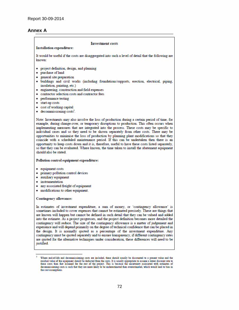
Report 30-09-2014
72
Annex A

Report 30-09-2014
73
Annex B – Exemplary investment data for DeNOx technologies
The following data of realised and estimated investments indicates the large range, a retrofit or a
new investment into DeNOx technologies might have. When reading the data, it has to be borne
in mind that most data reflects total project costs to the power plant operator and most projects
have been retrofits. For the scope of retrofit (incl. necessary additional modifications), the type of
costs which have been included and more details, please refer to the original literature.
EUR
/ k
We
EUR
/ k
Wth
Giv
en
Lite
ratu
re
Va
lues
M
in
Max
Min
Max
Ori
gin
al
Sou
rce
Min
Ma
x
Un
it
Co
un
try
Co
st Y
ear
Sup
pl.
Info
JEP
LNB
+SN
C
R
28
,51
28
,51
71
,29
71
,29
Ba
rmo
r,
20
06
20
20
GB
P/k
We
UK
20
07
IEA
LNB
2,3
5
2,3
5
5,8
8
5,8
8
Orf
an
ou
da
kis,
2
00
5
5 5
EUR
/kW
th
Gre
ece
20
05
IEA
LNB
5,8
3
20
,83
14
,58
52
,08
7
25
USD
/kW
e
UK
Hig
h E
nd
: OFA
IEA
LNB
5,8
3
30
,00
14
,58
75
,00
7 36
USD
/kW
e
US
Hig
h E
nd
: OFA
IEA
LNB
17
,14
17
,14
42
,85
42
,85
Sch
nec
k,
200
3
15
15
USD
/kW
e
Ca
na
da
200
3

Report 30-09-2014
74
JEP
SCR
11
4,0
6
18
5,3
5
28
5,1
5
46
3,3
7
Lite
ratu
re
Surv
ey
80
13
0
GB
P/k
We
US
20
07
JEP
SCR
28
5,1
5
29
9,4
1
71
2,8
7
74
8,5
2
Lite
ratu
re
Surv
ey
20
0
21
0
GB
P/k
We
US
20
07
Co
mp
lica
ted
JEP
SCR
52
,42
52
,42
13
1,0
4
13
1,0
4
Lite
ratu
re
Surv
ey
50
50
EUR
/kW
e
Fra
nce
20
07
JEP
SCR
85
,54
11
4,0
6
21
3,8
6
28
5,1
5
Ba
rmo
r, 2
00
6
60
80
GB
P/k
We
UK
20
07
low
eff
. to
h
igh
eff
. SC
R
IEA
SCR
23
,53
32
,94
58
,82
82
,35
Orf
an
ou
da
kis,
2
00
5
50
70
EUR
/kW
th
Gre
ece
20
05
IEA
SCR
50
,53
12
8,6
2
12
6,3
3
32
1,5
6
5
5
14
0
USD
/kW
e
US
IEA
SCR
41
,34
82
,69
10
3,3
6
20
6,7
2
4
5
90
USD
/kW
e
UK
IEA
SCR
91
,87
91
,87
229
,68
229
,68
1
00
100
USD
/kW
e
US
IEA
SCR
79
,99
182
,82
199
,96
457
,06
Mo
rris
, 200
3
70
160
USD
/kW
e
US
200
3
Ave
rag
e 1
10
USD
/kW
e

Report 30-09-2014
75
IEA
SCR
58
,20
12
8,0
5
14
5,5
1
32
0,1
2
US
EPA
, 20
02
50
11
0
USD
/kW
e
US
20
01
US
EPA
Co
st
Met
ho
do
log
y
IEA
SCR
82
,67
12
4,0
0
20
6,6
6
31
0,0
0
US
DO
E, 2
00
5
80
12
0
USD
/kW
e
US
20
04
IEA
SNC
R
7,0
6
14
,12
17
,65
35
,29
Orf
an
ou
da
kis,
2
00
5
15
30
EUR
/kW
th
Gre
ece
20
05
JEP
SNC
R
15
,83
15
,83
39
,57
39
,57
SNC
R r
eca
lcu
late
d
by
sub
tra
ctin
g t
he
LNB
ave
rag
e fr
om
LNB
+SN
CR
In
vest
men
t o
f B
arm
or,
20
06

Report 30-09-2014
76
Annex C – Exemplary investment data for ESP and PJFF technologies
The following data of realised and estimated investments indicates the large range, a retrofit or a
new investment into DeNOx technologies might have. When reading the data, it has to be borne
in mind that most data reflects total project costs to the power plant operator and most projects
have been retrofits. For the scope of retrofit (incl. necessary additional modifications), the type of
costs which have been included and more details, please refer to the original literature.
Min
Max
Curr
ency
Pow
er u
nit
Min
Max
RAIN
S20
0523
,80
23,8
0£
/kW
e16
,37
16,3
7
AEP
2005
28,0
028
,00
£/
kWe
19,2
619
,26
Nal
band
ian
[Sm
ith]
2006
53,0
080
,00
$/
kWe
18,6
128
,09
Nal
dand
ian
[Orf
anou
daki
s]20
0660
,50
60,5
0$
/kW
e21
,24
21,2
4
Nal
band
ian
2006
60,0
060
,00
$/
kWe
21,0
721
,07
Wor
ld b
ank
2001
36,0
036
$/
kWe
22,4
322
,43
IEA
1998
50,0
070
,00
$/
kWe
25,2
335
,32
Balc
ke D
urr
2008
19,7
021
,00
€/
kWth
18,8
620
,10
PM B
ART
det
erm
inat
ion
[Am
eric
an E
lect
ric P
ower
]20
0750
,00
50,0
0$
/kW
e38
,23
38,2
3
Serg
ent e
t Lun
dy20
1065
,21
87,5
6$
/kW
e18
,74
25,1
6
IEA
2000
4,80
45,0
0$
/kW
th7,
2668
,07
Wu
2001
3,90
16,5
0$
/kW
th6,
0825
,72
Lite
ratu
reCo
st Y
ear
EURO
201
0 /
kWth
Curr
ency
yea
r / p
ower
uni
t
ESP investment costs PJFF investment costs
Min
Max
Curr
ency
Pow
er u
nit
Min
Max
RAIN
S20
0517
,30
17,3
0£
/kW
e11
,90
11,9
0
AEP
2005
32,0
036
,00
£/
kWe
22,0
124
,77
Nal
band
ian
2006
70,7
070
,70
$/
kWe
24,8
224
,82
Nal
dand
ian
[Orf
anou
daki
s]20
0685
,00
85,0
0$
/kW
e29
,84
29,8
4
Wor
ld b
ank
2001
29,0
033
$/
kWe
18,0
720
,56
IEA
1998
40,0
060
,00
$/
kWe
20,1
830
,28
Balc
ke D
urr
2008
25,8
041
,80
€/
kWth
24,7
040
,01
Que
stio
nnar
y Pl
ant D
1983
13,3
013
,30
€/
kWth
23,3
323
,33
Zeve
nhov
en &
Kilp
inen
1982
9,65
9,65
$/
kWth
17,2
817
,28
Rubi
n19
8543
,00
43,0
0$
/kW
e38
,32
38,3
2
Sank
ey19
9719
,00
19,0
0$
/kW
th23
,86
23,8
6
IEA
1995
9,00
30,0
0$
/kW
th9,
9433
,15
Lite
ratu
reCo
st Y
ear
Curr
ency
yea
r / p
ower
uni
tEU
RO 2
010
/ kW
th
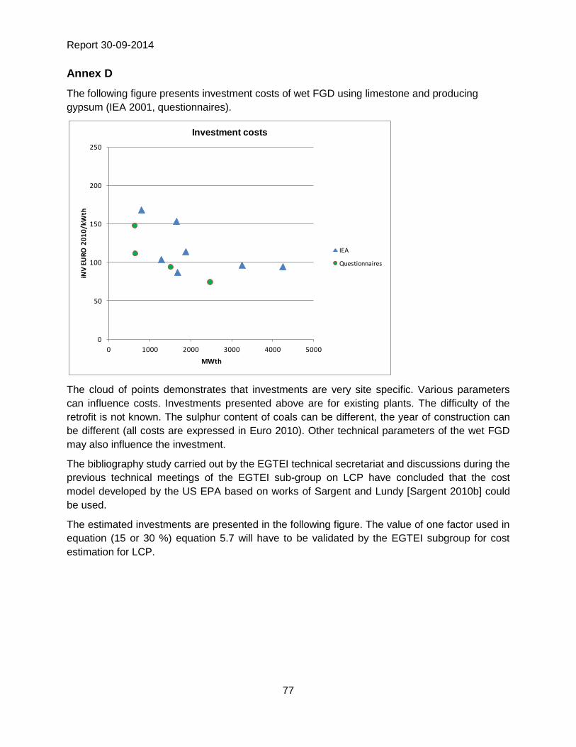
Report 30-09-2014
77
Annex D
The following figure presents investment costs of wet FGD using limestone and producing
gypsum (IEA 2001, questionnaires).
The cloud of points demonstrates that investments are very site specific. Various parameters
can influence costs. Investments presented above are for existing plants. The difficulty of the
retrofit is not known. The sulphur content of coals can be different, the year of construction can
be different (all costs are expressed in Euro 2010). Other technical parameters of the wet FGD
may also influence the investment.
The bibliography study carried out by the EGTEI technical secretariat and discussions during the
previous technical meetings of the EGTEI sub-group on LCP have concluded that the cost
model developed by the US EPA based on works of Sargent and Lundy [Sargent 2010b] could
be used.
The estimated investments are presented in the following figure. The value of one factor used in
equation (15 or 30 %) equation 5.7 will have to be validated by the EGTEI subgroup for cost
estimation for LCP.
0
50
100
150
200
250
0 1000 2000 3000 4000 5000
iNV
EU
RO
20
10
/kW
th
MWth
Investment costs
IEA
Questionnaires
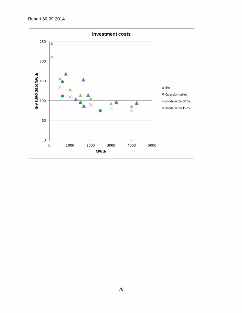
Report 30-09-2014
78
0
50
100
150
200
250
0 1000 2000 3000 4000 5000
iNV
EU
RO
20
10
/kW
th
MWth
Investment costs
IEA
Questionnaires
model with 30 %
model with 15 %
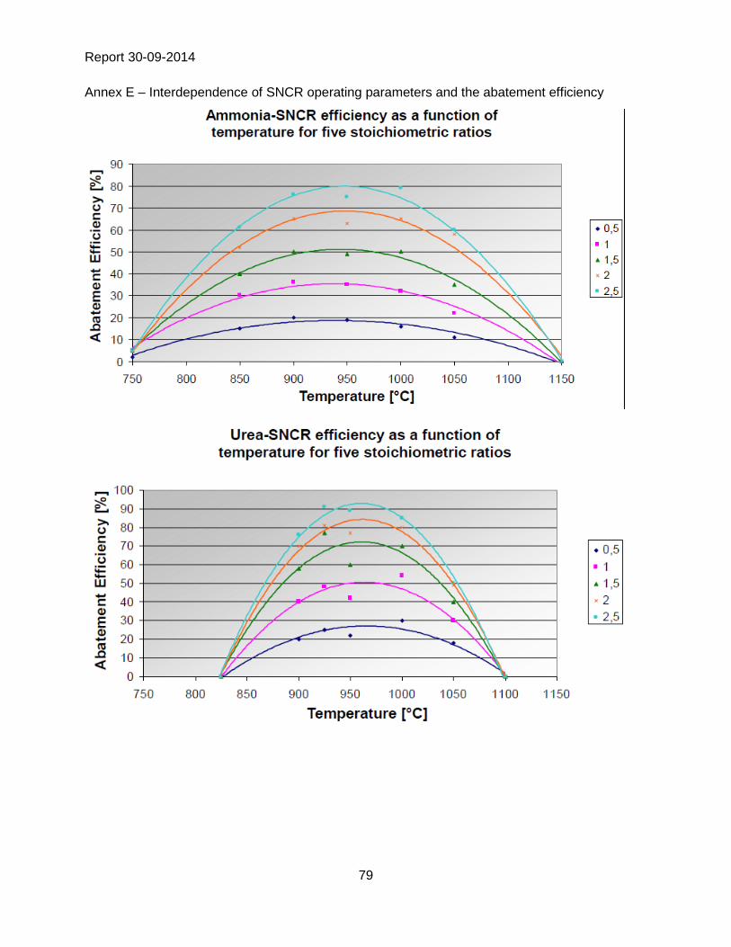
Report 30-09-2014
79
Annex E – Interdependence of SNCR operating parameters and the abatement efficiency


![diagram 5.1 [Converted] - Building Control NI · part of the flue serving an open-flued appliance. flue soot door debris collection space chimney appliance flue outlet appliance flue](https://img.pdfslide.us/doc/110x75/60ea4a68722f9641f22c1939/diagram-51-converted-building-control-ni-part-of-the-flue-serving-an-open-flued.jpg)