20

Estimation of Continuous-time Nonlinear Systems by using Unscented Kalman Filter

Min Zheng, Kenji Ikeda and Takao Shimomura The University of Tokushima

Japan

1. Introduction

The discrete-time model is often used for the system identification. However, the controlled plant is a continuous-time system in many cases. In addition, there are some disadvantages in the discrete-time model, such as the discrete-time model has a complex representation of the continuous-time model parameters, and can’t reflect the structure of the plant. Especially for the nonlinear system, if the sampling period is large, system nonlinearity will be enlarged, and the nonlinear discrete-time model can’t be identified well. Because of these reasons, the method for estimating the parameter of the continuous-time system from the sampled I/O data directly has attracted attention. Estimation in nonlinear system is very important, because almost all practical systems involve nonlinearities. The Unscented Kalman Filter (UKF) is a nonlinear estimation method, which propagates mean and covariance information through nonlinear transformation. It is accurate, and has superior implementation properties. Plant parameters can be estimated based on the UKF like algorithm by defining an augmented state as the state and the unknown parameters. As it is well known, the UKF uses sigma points to capture the statistics of a Gaussian random variable, instead of calculating the Jacobian matrices, and the UKF does not use linear approximation. Furthermore, it does not matter if the plant is based on continuous-time model, because the one-step-ahead estimate in continuous-time model can be calculated by numerical integration. From these reasons, it is possible to estimate the state and the parameters of a continuous-time system by using the UKF. In order to demonstrate the validity, the Rotary Pendulum is provided to estimate the unknown parameter of the continuous-time nonlinear system. For the numerical simulation, system parameters have been almost exactly estimated. From the experimental I/O data, system parameter has been estimated within one percent Relative Root Squared Error (RRSE) by using the UKF like algorithm.

2. Continuous-time model and discrete-time model

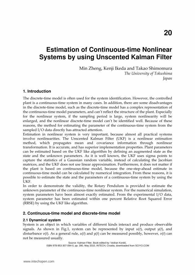
2.1 Dynamical system System is an object in which variables of different kinds interact and produce observable signals. As shown in Fig.1, system can be represented by input u(t), output y(t), and disturbance ν(t). As a general rule, u(t) and y(t) can be measured possibly, however, ν(t) can not be measured usually.

Source: Kalman Filter, Book edited by: Vedran Kordić, ISBN 978-953-307-094-0, pp. 390, May 2010, INTECH, Croatia, downloaded from SCIYO.COM

www.intechopen.com

Kalman Filter

374

Dynamical system is a system whose output depends not only the current input but also the past input.

Fig. 1. Dynamical system

In general, the dynamical system shown in Fig.1 is represented with n-dimensional state variables {x1 , . . . , xn} by a first-order differential equation as follows:

(1)

where {u1, . . . , ul} is l-dimensional system input signals, and m-dimensional output

(2)

can be measured. From

(3)

and vector functions

www.intechopen.com

Estimation of Continuous-time Nonlinear Systems by using Unscented Kalman Filter

375

(4)

eqs.(1) and (2) can be expressed briefly as follows

(5)

(6)

x(t) is called state vector, eqs.(1) and (5) are called state equation, and eqs.(2) and (6) are called output equations. In order to analyze the discrete-time model, f and g are assumed to be linear in section 2.2. At that time, eqs.(7) and (8) are used instead of eqs.(5) and (6)

(7)

(8)

where A(t) ∈ Rn×n,B(t) ∈ Rn×l,C(t) ∈ Rm×n,D(t) ∈ Rm×l respectively. It is called a time-varying linear system if the system is represented by eqs.(7) and (8). When A(t), B(t), C(t), D(t) are constant matrices and do not depend on the time variable t, the system

(9)

(10)

is called a time-invariant linear system. In many cases, D(t) = 0, because phase of a physical system always delays in high frequency range. Output eq.(8) can be changed as

(11)

Vis-a-vis the linear system, the system which is represented with eqs.(1), (2) or the eqs.(5), (6) is called a nonlinear system.

2.2 Continuous-time model and discrete-time model The behavior of a dynamic system evolves over time. The discrete-time model is often used for the system identification. However, in many cases the controlled plant is a continuous-time system, which its descriptive equations are defined for all values of time and the system dynamic properties shown by the differential equations. There are some properties of continuous-time model, 1. In the control design, the important parameters are easy to be grasped.

www.intechopen.com

Kalman Filter

376

2. If the physical structure of the plant is known, the mathematical continuous-time model can be obtained beforehand.

The focus in this chapter targets the modeling of continuous-time systems. As for the second property, if the differential equations of the continuous-time model can be obtained, the identification problem afterwards can be replaced by the parameter estimation problem. In many applications, particularly in physical modeling, the design of a discretetime model starts from the description of a physical continuous-time model by means of differential equations and constraints. Therefore, for this section, the continuous-time model is represented as

(12)

(13)

where u ∈ Rm, y ∈ Rl, A ∈ Rn×n, B ∈ Rn×m, C ∈ Rl×n. On the other hand, for performing a system by using a digital computer, it has become prerequisite to handle the sampled data. Discrete-time model is the mathematical model in which the I/O relation of the sampled data is shown by a difference equation. Corresponding to eqs.(14) and (15), the discrete-time model can be described by

(14)

(15)

Similarly to the continuous-time model, xk, uk and yk are state variable vector, input and output at a time step k respectively. And G ∈ Rn×m and H(=C) ∈ Rl×n are the system matrices of the discrete-time model. The solution of eq.(14) can be solved as

(16)

where t0 is the initial time. Let tk, k=0, 1, . . ., denote the sampling time. If the input u(t) is a constant uk for the sampling interval [tk, tk+1), i.e.

(17)

Then

(18)

can be obtained. Here, assume tk+1 − tk = Δ(const.), the discrete-time system representated as follow

www.intechopen.com

Estimation of Continuous-time Nonlinear Systems by using Unscented Kalman Filter

377

(19)

where

(20)

Δ is the sampling period. For zero-order hold of the sampling, it is possible to calculate without the approximate error. However, if unlimitedly reduces Δ,

(21)

F and G approach to identity matrix and zero matrix, regardless of the elements of A and B. Moreover, if the obtained discrete-time model is clear to identity matrix or zero matrix, the backward calculation from the discrete-time model to the continuous-time model becomes numerically unstable. Therefore, for the discrete-time model, the value of the model depends on the sampling period. And it is not limited to represent the dynamics of the actual system accurately, though the sampling period be diminished simply. In a summary, for the discrete-time model and continuous-time model, there are some problems 1. The discrete-time model does not reflect the structure of the plant. 2. The discrete-time model has a complex representation of the continuous-time model

parameters. 3. Especially for the nonlinear system, if the sampling period is large, system nonlinearity

will be enlarged, and the nonlinear discrete-time model can’t be identified well. Because of these reasons, the method for estimating the parameter of the continuous-time system from the sampled I/O data directly has attracted attention.

3. Unscented Kalman filter

Estimation in nonlinear system is very important because many practical systems involve nonlinearities. The Extended Kalman Filter (EKF) which applies the KF to nonlinear system by linearizing all nonlinear models, has become a most widely used method for estimation of nonlinear system. However, more than 35 years of experience in the estimation community, although the EKF maintains the elegant and computationally efficient recursive update form of the KF, it suffers a number of serious limitations. 1. Only reliable for systems which are almost linear on the time scale of the updates. 2. Linearization can be applied only if the Jacobian matrix exists. However, this is not

always the case. 3. Calculating Jacobian matrices can be a very difficult and error-prone process. It means the EKF is difficult to implement, difficult to tune, and the reliability is limited. To address the limitations, the Unscented Kalman Filter (UKF) was proposed by Julier and Uhlmann in 1996.

www.intechopen.com

Kalman Filter

378

The UKF is a nonlinear estimation method which propagates mean and covariance information of the parameter recursively through nonlinear transformation. As it is well known, the UKF is a straightforward extension of the Unscented Transformation (UT) to the recursive estimations. It uses sigma points to capture the statistics instead of calculating the Jacobian matrices, and the UKF does not use the linear approximation of functions. It is accurate, and has superior implementation properties. As a nonlinear estimation method, the UKF has been widely applied in nonlinear control applications.

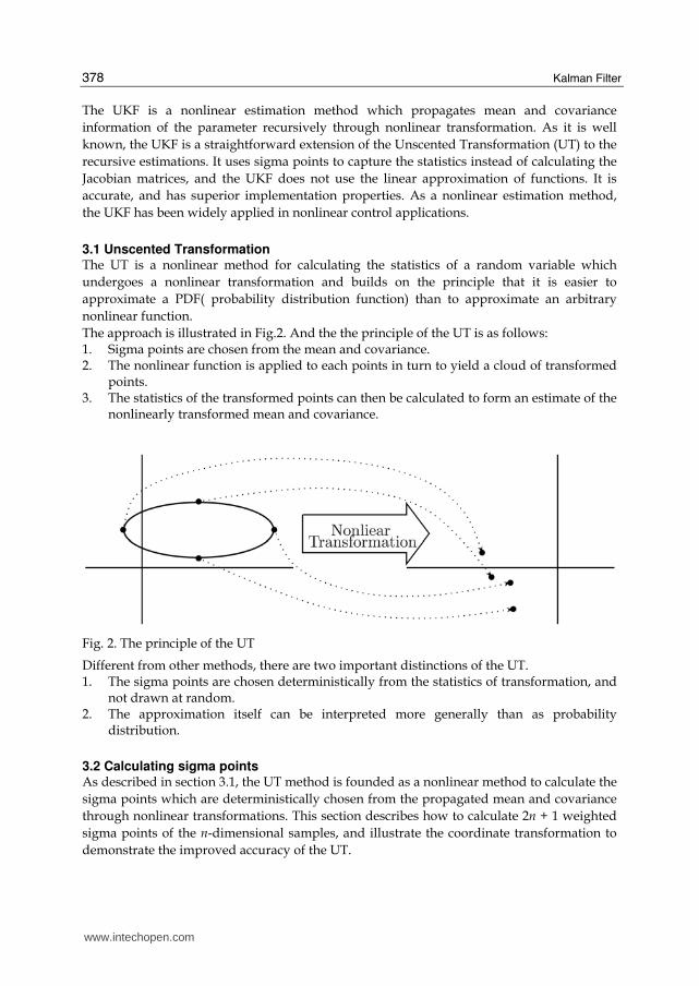
3.1 Unscented Transformation The UT is a nonlinear method for calculating the statistics of a random variable which undergoes a nonlinear transformation and builds on the principle that it is easier to approximate a PDF( probability distribution function) than to approximate an arbitrary nonlinear function. The approach is illustrated in Fig.2. And the the principle of the UT is as follows: 1. Sigma points are chosen from the mean and covariance. 2. The nonlinear function is applied to each points in turn to yield a cloud of transformed

points. 3. The statistics of the transformed points can then be calculated to form an estimate of the

nonlinearly transformed mean and covariance.

Fig. 2. The principle of the UT

Different from other methods, there are two important distinctions of the UT. 1. The sigma points are chosen deterministically from the statistics of transformation, and

not drawn at random. 2. The approximation itself can be interpreted more generally than as probability

distribution.

3.2 Calculating sigma points As described in section 3.1, the UT method is founded as a nonlinear method to calculate the sigma points which are deterministically chosen from the propagated mean and covariance through nonlinear transformations. This section describes how to calculate 2n + 1 weighted sigma points of the n-dimensional samples, and illustrate the coordinate transformation to demonstrate the improved accuracy of the UT.

www.intechopen.com

Estimation of Continuous-time Nonlinear Systems by using Unscented Kalman Filter

379

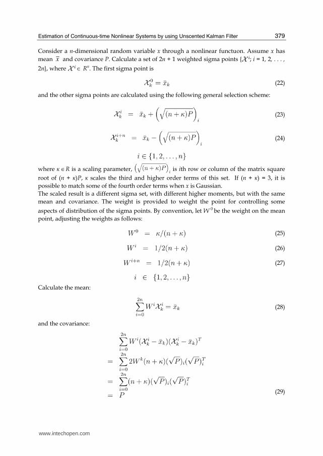
Consider a n-dimensional random variable x through a nonlinear functuon. Assume x has mean x and covariance P. Calculate a set of 2n + 1 weighted sigma points { ; i = 1, 2, . . . ,

2n}, where ∈ Rn. The first sigma point is

(22)

and the other sigma points are calculated using the following general selection scheme:

(23)

(24)

where κ ∈R is a scaling parameter, is ith row or column of the matrix square root of (n + κ)P, κ scales the third and higher order terms of this set. If (n + κ) = 3, it is possible to match some of the fourth order terms when x is Gaussian. The scaled result is a different sigma set, with different higher moments, but with the same mean and covariance. The weight is provided to weight the point for controlling some aspects of distribution of the sigma points. By convention, let W 0 be the weight on the mean point, adjusting the weights as follows:

(25)

(26)

(27)

Calculate the mean:

(28)

and the covariance:

(29)

www.intechopen.com

Kalman Filter

380

From the results, the mean and covariance of are same to them of xk is found.

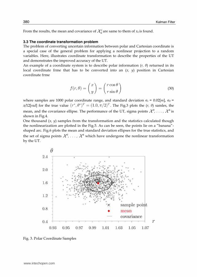
3.3 The coordinate transformation problem The problem of converting uncertain information between polar and Cartesian coordinate is a special case of the general problem for applying a nonlinear projection to a random variables. Here, illustrates coordinate transformation to describe the properties of the UT and demonstrates the improved accuracy of the UT. An example of a coordinate system is to describe polar information (r, θ) returned in its local coordinate frme that has to be converted into an (x, y) position in Cartesian coordinate frme

(30)

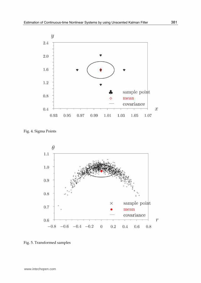
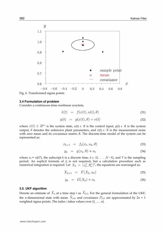
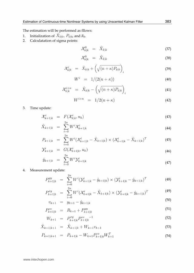
where samples are 1000 polar coordinate range, and standard deviation pr = 0.02[m], pθ = π/12[rad] for the true value . The Fig.3 plots the (r, θ) samles, the

mean, and the covariance ellipse. The performance of the UT, sigma points 0, . . . , 4 is shown in Fig.4. One thousand (x, y) samples from the transformation and the statistics calculated though the nonlinearization are plotted in the Fig.5. As can be seen, the points lie on a ”banana”-shaped arc. Fig.6 plots the mean and standard deviation ellipses for the true statistics, and the set of sigma points 0, . . . , 4 which have undergone the nonlinear transformation by the UT.

Fig. 3. Polar Coordinate Samples

www.intechopen.com

Estimation of Continuous-time Nonlinear Systems by using Unscented Kalman Filter

381

Fig. 4. Sigma Points

Fig. 5. Transformed samples

www.intechopen.com

Kalman Filter

382

Fig. 6. Transformed sigma points

3.4 Formulation of problem Consider a continuous-time nonlinear sysytem,

(31)

(32)

where is the system state, u(t) ∈ R is the control input, y(t) ∈ R is the system output, θ denotes the unknown plant parameters, and ν(t) ∈ R is the measurement noise with zero mean and its covariance matrix R. The discrete-time model of the system can be represented as:

(33)

(34)

where xk = x(kT), the subscript k is a discrete time, k ∈ {1, . . . ,N −1}, and T is the sampling period. An explicit formula of fd is not required, but a calculation procedure such as numerical integration is required. Let , the equations are rearranged as:

(35)

(36)

3.5. UKF algorithm

Denote an estimate of at a time step l as . For the general formulation of the UKF, the n-dimensional state with mean and covariance are approximated by 2n + 1 weighted sigma points. The index i takes values over {1, ... , n}.

www.intechopen.com

Estimation of Continuous-time Nonlinear Systems by using Unscented Kalman Filter

383

The estimation will be performed as fllows: 1. Initialization of , and R0. 2. Calculatation of sigma points:

(37)

(38)

(39)

(40)

(41)

(42)

3. Time update:

(43)

(44)

(45)

(46)

(47)

4. Measurement update:

(48)

(49)

(50)

(51)

(52)

(53)

(54)

www.intechopen.com

Kalman Filter

384

Summarily, the UKF uses sigma points to capture the mean and covariance of a Gaussian random variable, instead of calculating the Jacobian matrices. Plant parameters can be estimated based on the UKF like algorithm by augmenting the state with the unknown parameters. Furthermore, it does not matter if the estimation is based on continuous-time model, because the one-step-ahead estimate in continuous-time model can be calculated by numerical integration. From these reasons, it is possible to estimate the state and the parameters of a continuous-time system by using the UKF like algorithm.

4. Numerical example

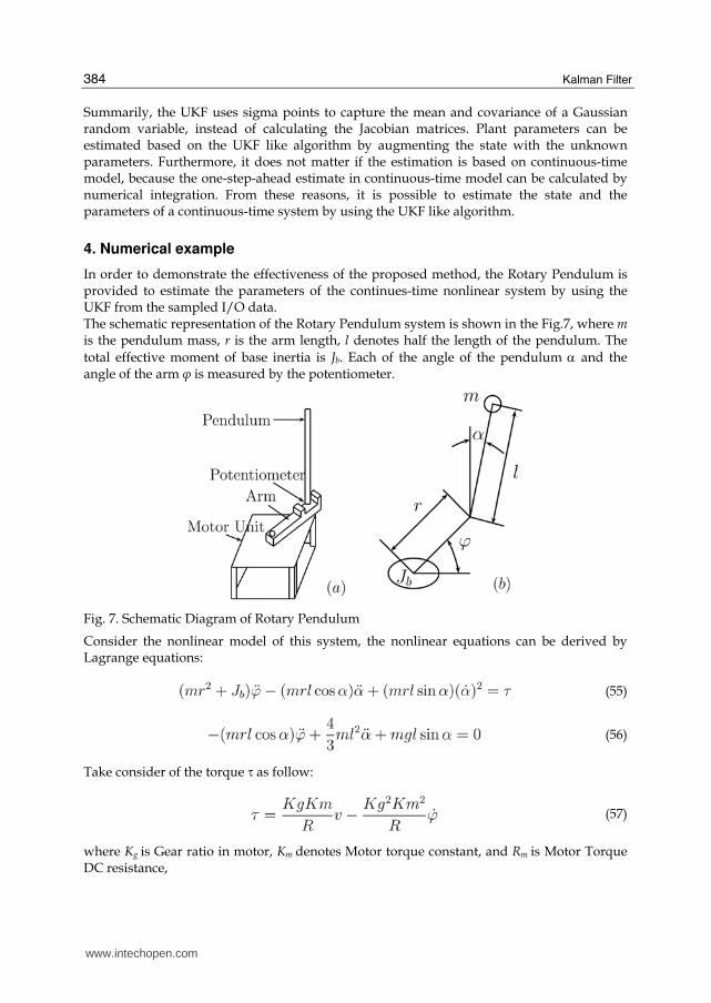
In order to demonstrate the effectiveness of the proposed method, the Rotary Pendulum is provided to estimate the parameters of the continues-time nonlinear system by using the UKF from the sampled I/O data. The schematic representation of the Rotary Pendulum system is shown in the Fig.7, where m is the pendulum mass, r is the arm length, l denotes half the length of the pendulum. The total effective moment of base inertia is Jb. Each of the angle of the pendulum α and the angle of the arm φ is measured by the potentiometer.

Fig. 7. Schematic Diagram of Rotary Pendulum

Consider the nonlinear model of this system, the nonlinear equations can be derived by Lagrange equations:

(55)

(56)

Take consider of the torque q as follow:

(57)

where Kg is Gear ratio in motor, Km denotes Motor torque constant, and Rm is Motor Torque DC resistance,

www.intechopen.com

Estimation of Continuous-time Nonlinear Systems by using Unscented Kalman Filter

385

and rearrange the equations into the state space representation given as:

(58)

where

(59)

(60)

The parameters of the plant can be estimated from eq.(58) by using the UKF like algorithm. The numerical values of parameters are provided in Tabel.1.

Table 1. Parameters of the experiment Rotary Pendulum system

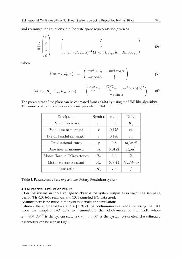
4.1 Numerical simulation result Offer the system an input voltage to observe the system output as in Fig.8. The sampling period T is 0.008668 seconds, and 1001 sampled I/O data used. Assume there is no noise in the system to make the simulations. Estimate the augmented state X = [x, θ] of the continuous-time model by using the UKF from the sampled I/O data to demonstrate the effectiveness of the UKF, where

x = is the system state and θ = is the system parameter. The estimated

parameters can be seen in Fig.9.

www.intechopen.com

Kalman Filter

386

Fig. 8. Input and Output of the Rotary Pendulum system

Fig. 9. Estimated parameters

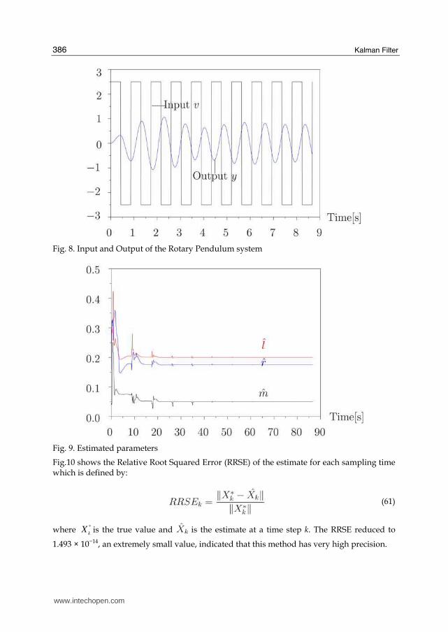
Fig.10 shows the Relative Root Squared Error (RRSE) of the estimate for each sampling time which is defined by:

(61)

where *

kX is the true value and is the estimate at a time step k. The RRSE reduced to

1.493 × 10−14, an extremely small value, indicated that this method has very high precision.

www.intechopen.com

Estimation of Continuous-time Nonlinear Systems by using Unscented Kalman Filter

387

Fig. 10. RRSE of the parameter esimation

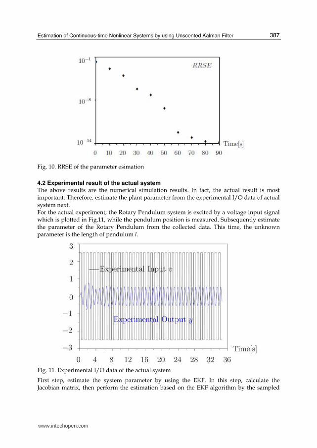
4.2 Experimental result of the actual system The above results are the numerical simulation results. In fact, the actual result is most important. Therefore, estimate the plant parameter from the experimental I/O data of actual system next. For the actual experiment, the Rotary Pendulum system is excited by a voltage input signal which is plotted in Fig.11, while the pendulum position is measured. Subsequently estimate the parameter of the Rotary Pendulum from the collected data. This time, the unknown parameter is the length of pendulum l.

Fig. 11. Experimental I/O data of the actual system

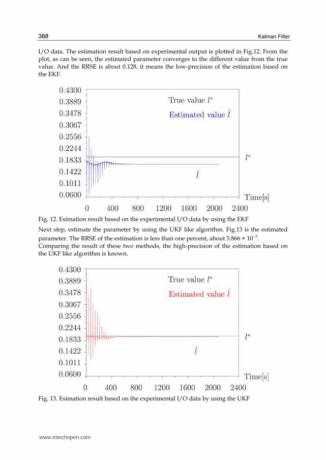
First step, estimate the system parameter by using the EKF. In this step, calculate the Jacobian matrix, then perform the estimation based on the EKF algorithm by the sampled

www.intechopen.com

Kalman Filter

388

I/O data. The estimation result based on experimental output is plotted in Fig.12. From the plot, as can be seen, the estimated parameter converges to the different value from the true value. And the RRSE is about 0.128, it means the low-precision of the estimation based on the EKF.

Fig. 12. Esimation result based on the experimental I/O data by using the EKF

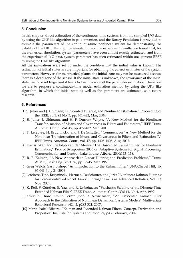
Next step, estimate the parameter by using the UKF like algorithm. Fig.13 is the estimated parameter. The RRSE of the estimation is less than one percent, about 5.866 × 10−3. Comparing the result of these two methods, the high-precision of the estimation based on the UKF like algorithm is known.

Fig. 13. Esimation result based on the experimental I/O data by using the UKF

www.intechopen.com

Estimation of Continuous-time Nonlinear Systems by using Unscented Kalman Filter

389

5. Conclusion

In this chapter, direct estimation of the continuous-time systems from the sampled I/O data by using the UKF like algorithm is paid attention, and the Rotary Pendulum is provided to estimate the parameters of the continuous-time nonlinear system for demonstrating the validity of the UKF. Through the simulation and the experiment results, we found that, for the numerical simulation, system parameters have been almost exactly estimated, and from the experimental I/O data, system parameter has been estimated within one percent RRSE by using the UKF like algorithm. All the simulations were set up under the condition that the initial value is known. The estimation of initial states is very important for obtaining the correct estimates of the system parameters. However, for the practical plants, the initial state may not be measured because there is a dead zone of the sensor. If the initial state is unknown, the covariance of the initial state has to be set large, and it leads to low precision of the parameter estimation. Therefore, we are to propose a continuous-time model estimation method by using the UKF like algorithm, in which the initial state as well as the paramters are estimated, as a future research.

6. References

[1] S. Julier and J. Uhlmann, ”Unscented Filtering and Nonlinear Estimation,” Proceeding of the IEEE, vol1. 92 No. 3, pp. 401-422, Mar, 2004.

[2] S. Julier, J. Uhlmann, and H. F. Durrant Whyte, ”A New Method for the Nonlinear Transfor- mation of Means and Covariances in Filters and Estimators,” IEEE Trans. Automat. Contr., Vol. 45, pp. 477-482, Mar, 2000.

[3] T. Lefebvre, H. Bruyninckx, and J. De Schutter, ”Comment on ”A New Method for the Nonlinear Transformation of Means and Covariances in Filters and Estimations”,” IEEE Trans. Automat. Contr., vol. 47, pp. 1406-1408, Aug, 2002.

[4] Eric A. Wan and Rudolph van der Merwe ”The Unscented Kalman Filter for Nonlinear Estimation,” Proc of Symposium 2000 on Adaptive Systems for Signal Processing, Communication and Control, Lake Louise, Alberta, 2000:153- 158.

[5] R. E. Kalman, ”A New Approach to Linear Filtering and Prediction Problems,” Trans. ASME J.Basic Eng., vol1. 82, pp. 35-45, Mar, 1960.

[6] Greg Welch, Gary Bishop, ”An Introduction to the Kalman Filter” UNCChapel Hill, TR 95-041, July 24, 2006

[7] Lefebvre, Tine, Bruyninckx, Herman, De Schutter, and Joris: ”Nonlinear Kalman Filtering for Force-Controlled Robot Tasks”, Springer Tracts in Advanced Robotics, Vol. 19, Nov, 2005.

[8] K. Reif, S. Günther, E. Yaz, and R. Unbehuaen: ”Stochastic Stability of the Discrete-Time Extended Kalman Filter”, IEEE Trans. Automat. Contr., Vol.44, No.4, Apr, 1999.

[9] Sy-Miin Chow, Emilio Ferrer, John R. Nesselroade, ”An Unscented Kalman Filter Approach to the Estimation of Nonlinear Dynamical Systems Models” Multivariate Behavioral Research, v42.n2, p283-321, 2007.

[10] Maria Isabel Ribeiro, ”Kalman and Extended Kalman Filters: Concept, Derivation and Properties” Institute for Systems and Robotics, p43, February, 2004.

www.intechopen.com

Kalman Filter

390

[11] Joseph J. LaVio la Jr., ”A Comparison of Unscented and Extended Kalman Filter for Estimating Quaternion Motion” American Control Conference, 2435-2440 vol.3, Jun, 2003.

[12] Lonnie C. Ludeman, ”Random Processes: Filtering, Estimation, and Detection”, ISBN 7-121-00866-1, January, 2003.

[13] Kenji Ikeda, Yoshio Mogami and Takao Shimomura, ”Continuous-time model identification by using adaptive observer, — Estimation of the initial state —”, Proc. of SICE-ICCAS 2006, pp.1796-1799, Busan, Oct, 2006.

[14] Kenji Ikeda, Yoshio Mogami and Takao Shimomura, ”Continuous-time model identification by using adaptive observer”, of 13th IFAC Symposium on System Identification, pp.325-330, Rotterdam, Aug, 2003.

[15] Rudolph van der Merwe and Eric A. Wan, ”Sigma-Point Kalman Filters for Intergrated Navigation”, Proceedings of the 60th Annual Meeting, pp.641-654, Jun, 2004.

[16] S. J. Julier: ”Reduced Sigma Point Filters for the Propagation of Means and Covariances Through Nonlinear Transformations”, available in http://citeseer.ist.psu.edu/

[17] S. J. Julier: ”The Scaled Unscented Transformation”, available in http://citeseer.ist.psu.edu/

[18] S. J. Julier, and J. K. Uhlmann: ” A Consistent, Debiased Method for Converting Between Polar and Cartesian Coordinate Systems”, available in http://citeseer.ist.psu.edu/

[19] S. J. Julier, and J. K. Uhlmann: ”A New Extension of the Kalman Filter to Nonlinear Systems”, available in http://citeseer.ist.psu.edu

[20] Brian D.O. Anderson, and John B. Moore, ”Optimal Filtering”, Dover 0-486- 43938-0 [21] Mohinder S. Grewal, Angus P. Andrews, ”Kalman Filtering: theory and practice Using

Matlab, second edition”, Wiley-Interscience, Jan, 2001. [22] Karl J.Åström, BJörnWittenmark, ”Computer-Controlled Systems: theory and design,

second edition”, Prentice Hall, November, 2006.

www.intechopen.com

Kalman FilterEdited by Vedran Kordic

ISBN 978-953-307-094-0Hard cover, 390 pagesPublisher InTechPublished online 01, May, 2010Published in print edition May, 2010

InTech EuropeUniversity Campus STeP Ri Slavka Krautzeka 83/A 51000 Rijeka, Croatia Phone: +385 (51) 770 447 Fax: +385 (51) 686 166www.intechopen.com

InTech ChinaUnit 405, Office Block, Hotel Equatorial Shanghai No.65, Yan An Road (West), Shanghai, 200040, China

Phone: +86-21-62489820 Fax: +86-21-62489821

The Kalman filter has been successfully employed in diverse areas of study over the last 50 years and thechapters in this book review its recent applications. The editors hope the selected works will be useful toreaders, contributing to future developments and improvements of this filtering technique. The aim of this bookis to provide an overview of recent developments in Kalman filter theory and their applications in engineeringand science. The book is divided into 20 chapters corresponding to recent advances in the filed.

How to referenceIn order to correctly reference this scholarly work, feel free to copy and paste the following:

Min Zheng, Kenji Ikeda and Takao Shimomura (2010). Estimation of Continuous-Time Nonlinear Systems byUsing Unscented Kalman Filter, Kalman Filter, Vedran Kordic (Ed.), ISBN: 978-953-307-094-0, InTech,Available from: http://www.intechopen.com/books/kalman-filter/estimation-of-continuous-time-nonlinear-systems-by-using-unscented-kalman-filter

© 2010 The Author(s). Licensee IntechOpen. This chapter is distributedunder the terms of the Creative Commons Attribution-NonCommercial-ShareAlike-3.0 License, which permits use, distribution and reproduction fornon-commercial purposes, provided the original is properly cited andderivative works building on this content are distributed under the samelicense.