Estimation of Arterial Measures of Effectiveness with ...xuanyg/doc/Argote_Christofa_Xuan... · Estimation of Arterial Measures of Effectiveness with Connected Vehicle Data ... the

Paper No. 12-1493

Estimation of Arterial Measures of Effectiveness with Connected Vehicle Data

Juan Argote (corresponding author)Department of Civil and Environmental Engineering

Institute of Transportation Studies109 McLaughlin Hall, University of California, Berkeley, CA 94720

Phone: +1(510) 857-4547, Email: [email protected]

Eleni ChristofaDepartment of Civil and Environmental Engineering



Yiguang XuanDepartment of Civil and Environmental Engineering



andAlexander Skabardonis, Ph.D.

Department of Civil and Environmental EngineeringInstitute of Transportation Studies

109 McLaughlin Hall, University of California, Berkeley, CA 94720Phone: +1(510) 642-9166, Fax: +1(510) 642-1246, Email: [email protected]

91st Annual MeetingTransportation Research Board

Washington, D.C.January 22–26, 2012

Word Count: 4,314Figures/Tables: 12Total: 7,314

Revised November 8th, 2011

TRB 2012 Annual Meeting Paper revised from original submittal.

Argote, Christofa, Xuan, and Skabardonis 1

ABSTRACT

The Connected Vehicle technology is a promising mobile data source for improving real-time traffic con-ditions monitoring and control. This paper presents estimation methods for a variety of measures of effec-tiveness both at the arterial and intersection level (e.g., average speed, acceleration noise, queue length).These performance measures are essential for determining traffic conditions and improving signal controlstrategies in real-time. The estimation methods are tested with two datasets comprising of various trafficconditions: undersaturated and oversaturated and the minimum penetration rate requirements for accurateMOE estimates are determined. These reveal that for oversaturated conditions the required penetration ratesare smaller than those for undersaturated. Finally, an application of the queue length estimation as a triggerfor alternative real-time control strategies is presented. The developed method determines the last observedvehicle distance threshold that activates the alternative signal plan as a function of the Connected Vehiclepenetration rate.



INTRODUCTION

The Connected Vehicle (CV) technology is a promising mobile data source that can provide real-time infor-mation necessary for evaluating traffic conditions on a network. Such real-time information can be used todesign and evaluate more efficient control strategies for signalized networks. However, the ability to use suchdata depends on the penetration rate of equipped vehicles. It is therefore critical to develop a comprehen-sive methodology that uses CV data under different penetration rates to estimate Measures of Effectiveness(MOEs). In addition, there is a need to estimate minimum penetration rate requirements that allow accurateestimates under different traffic conditions. This is particularly useful to determine which MOEs can beused for a specific real-time application under different market penetration of the traffic conditions and theCV technology.

Several studies have been conducted in estimating MOEs with the help of CV or probe data. Themajority of these studies have focused on the estimation of queue length (1, 2, 3, 4), which is a commonlyused measure for designing and evaluating control strategies and is difficult to estimate with static sensors.Probe vehicle data were used by Comert and Cetin (1) who studied the distribution of average queue lengthsassuming known penetration rate, while Venkatanarayana et al. (2) estimated queue lengths by using theposition of the last IntelliDriveSM equipped vehicle in queue (i.e., maximum likelihood estimation). Haoand Ban (3) and Cheng et al. (4) used kinematic wave theory to estimate queue lengths. However, onlyComert and Cetin (1) considered the impact of the penetration rate of the equipped vehicles on the estimationaccuracy.

However, none of the studies provides a comprehensive description of the estimation process fora wide range of MOEs and traffic conditions. In addition, the penetration rate thresholds that ensure ac-curate MOEs estimates for real-time traffic control applications have not been identified in the literature.In this paper we explicitly address these issues. We developed and tested algorithms for estimating MOEsfrom CV trajectory data, and identified penetration rate requirements for accurate MOE estimates in bothundersaturated and oversaturated traffic conditions.

The rest of the paper is organized as follows. First, the two datasets used in the analysis are brieflydescribed. Next, the methods for estimating arterial MOEs are presented and the minimum penetration raterequirements for accurate estimates are identified. Estimation of the main intersection level MOE, i.e. queuelength, follows and minimum penetration rates for accurate estimates are also identified. Next, we presenta method for determining distance from the intersection thresholds for the last observed vehicle, which canbe used to identify queue spillovers, is investigated. The last section summarizes the study findings andoutlines future research.

TEST SITES

The impact of the CV technology penetration rate on the accuracy of the MOEs has been estimated withthe use of actual vehicle trajectories obtained from the Next Generation Simulation (NGSIM) program (5)and simulated trajectories from El Camino Real, a major arterial in the San Francisco Bay Area. TheNGSIM dataset was used to test the proposed estimation procedures for undersaturated traffic conditions,the conditions where the queues are completely dissipated at within each signal cycle. Since no real datawas available for oversaturated traffic conditions, when not all the demand can be served within the cycleand residual queues form, the El Camino simulated data was used. A more detailed description of the twodatasets follows.

NGSIM Data: Peachtree Street, Atlanta, GA

NGSIM data collected at Peachtree Street, Atlanta, GA for four signalized intersections have been chosenfor this study. The NGSIM dataset consists of vehicle trajectories; the format includes vehicle ID, time,position, lane, speed, and acceleration. All data are available at a resolution of ∆T = 0.1 seconds. In



addition, vehicle type, vehicle length, and their origins and destinations are available. The traffic signals’settings (cycle length, green, yellow, and offsets) are also known. The data used in this study were collectedfrom 12:45 to 13:00 and present only undersaturated conditions. Since the MOEs estimated in this paperdescribe the traffic conditions for a given direction, only the trajectories of vehicles traveling northbound ofthe main arterial were considered. This resulted in a total of 228 vehicle trajectories processed.

Simulated Data: El Camino Real, San Francisco Bay Area, CA

An existing microsimulation model of El Camino Real in VISSIM was used to obtain data for oversaturatedtraffic conditions. The selected arterial section includes five intersections starting at Cambridge and endingat Page Mill for the southbound direction. The simulation included 30 minutes of warm-up period so that thearterial could be loaded gradually and the next 15 minutes were used in the analysis. The trajectories wereexported with the same fields and resolution as the NGSIM dataset. A total of 1,332 vehicle trajectorieswere processed.

ARTERIAL MEASURES OF EFFECTIVENESS

This section presents the estimation of arterial-based MOEs for different market penetration rate values, p,for the CV equipped vehicles. For each of the p values considered, 10,000 samples were obtained whereeach vehicle trajectory was sampled following a Bernoulli trial with probability p. Box plots were used toreveal the arterial MOE estimate variation and identify the minimum p required to accurately estimate agiven MOE for both undersaturated and oversaturated conditions. On each box, the central mark representsthe median of the estimates, while the edges of the box show the 25th and 75th percentiles (see for exampleFigure 1). These plots also include a whisker range that extends 1.5 times the distance between the 25th and75th percentiles at both extremes of the box. A penetration rate was considered acceptable if the whiskerrange, which corresponds to ±2.7 the standard deviation of the estimate, laid within a 10% of the averagevalue for the ground truth. If the estimation errors are assumed to be normally distributed, this criteriaensures that the MOE estimate would lay within a 10% of the ground truth with a probability of 0.9965.

Average Speed

The average speed for all lanes in the observed direction for a single sample was obtained by using Edie’sgeneralized average speed definition (6), including all the vehicles in the sample:

v̄ =

S

∑i=1

li

S

∑i=1

ti

. (1)

Where:

S is the total number of vehicle trajectories sampled,

li is the total distance traveled by vehicle i,

ti is the total time spent by that vehicle to traverse li.

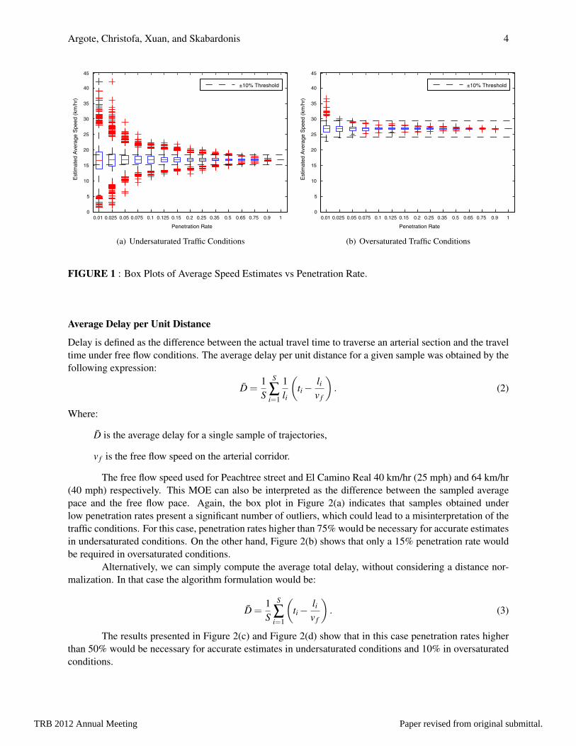
Figure 1 shows the boxplot of the average speeds for different penetration rates for both the NGSIMand the simulated data. Based on the threshold of ±2.7σ defined above, Figure 1 reveals that penetrationrates higher than 35% are necessary to provide accurate speed estimates for an arterial for undersaturatedtraffic conditions and higher than 5% for ovesaturated traffic condtions.



0.01 0.025 0.05 0.075 0.1 0.125 0.15 0.2 0.25 0.35 0.5 0.65 0.75 0.9 10

5

10

15

20

25

30

35

40

45

Penetration Rate

Est

imat

ed A

vera

ge S

peed

(km

/hr)

±10% Threshold

(a) Undersaturated Traffic Conditions

0.01 0.025 0.05 0.075 0.1 0.125 0.15 0.2 0.25 0.35 0.5 0.65 0.75 0.9 10

5

10

15

20

25

30

35

40

45

Penetration Rate

Est

imat

ed A

vera

ge S

peed

(km

/hr)

±10% Threshold

(b) Oversaturated Traffic Conditions

FIGURE 1 : Box Plots of Average Speed Estimates vs Penetration Rate.

Average Delay per Unit Distance

Delay is defined as the difference between the actual travel time to traverse an arterial section and the traveltime under free flow conditions. The average delay per unit distance for a given sample was obtained by thefollowing expression:

D̄ =1S

S

∑i=1

1li

(ti−

liv f

). (2)

Where:

D̄ is the average delay for a single sample of trajectories,

v f is the free flow speed on the arterial corridor.

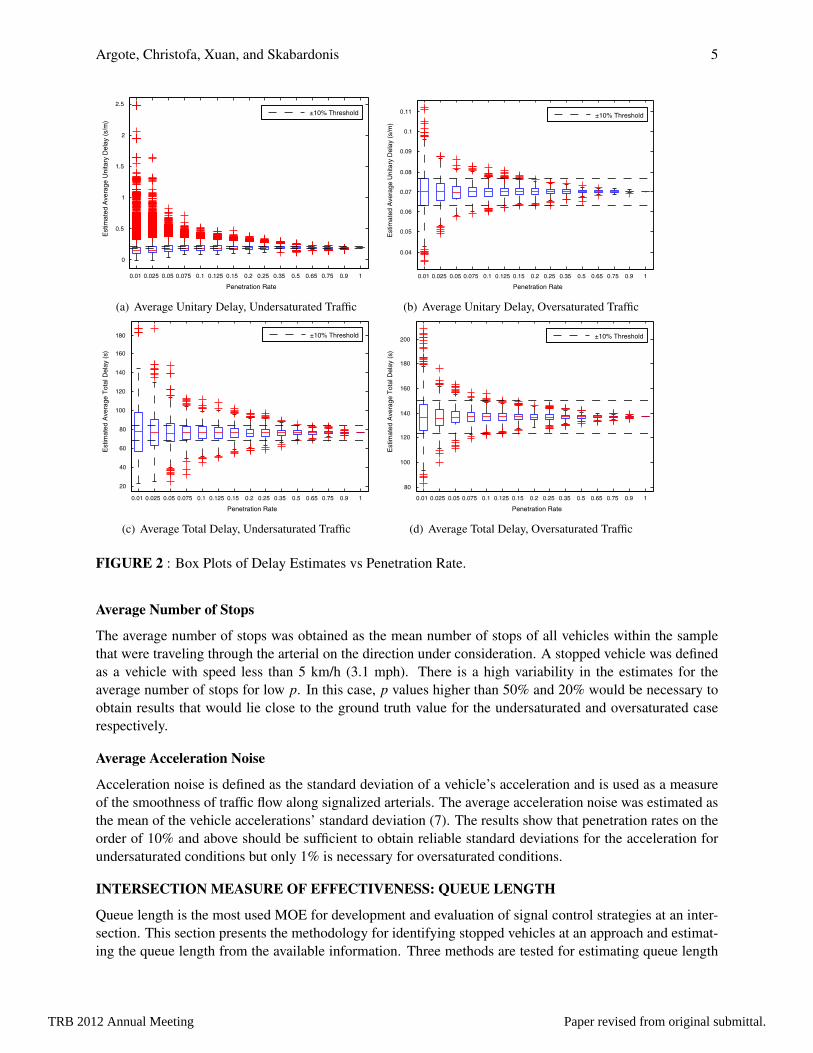
The free flow speed used for Peachtree street and El Camino Real 40 km/hr (25 mph) and 64 km/hr(40 mph) respectively. This MOE can also be interpreted as the difference between the sampled averagepace and the free flow pace. Again, the box plot in Figure 2(a) indicates that samples obtained underlow penetration rates present a significant number of outliers, which could lead to a misinterpretation of thetraffic conditions. For this case, penetration rates higher than 75% would be necessary for accurate estimatesin undersaturated conditions. On the other hand, Figure 2(b) shows that only a 15% penetration rate wouldbe required in oversaturated conditions.

Alternatively, we can simply compute the average total delay, without considering a distance nor-malization. In that case the algorithm formulation would be:

D̄ =1S

S

∑i=1

(ti−

liv f

). (3)

The results presented in Figure 2(c) and Figure 2(d) show that in this case penetration rates higherthan 50% would be necessary for accurate estimates in undersaturated conditions and 10% in oversaturatedconditions.



0.01 0.025 0.05 0.075 0.1 0.125 0.15 0.2 0.25 0.35 0.5 0.65 0.75 0.9 1

0

0.5

1

1.5

2

2.5

Penetration Rate

Est

imat

ed A

vera

ge U

nita

ry D

elay

(s/

m)

±10% Threshold

(a) Average Unitary Delay, Undersaturated Traffic

0.01 0.025 0.05 0.075 0.1 0.125 0.15 0.2 0.25 0.35 0.5 0.65 0.75 0.9 1

0.04

0.05

0.06

0.07

0.08

0.09

0.1

0.11

Penetration Rate

Est

imat

ed A

vera

ge U

nita

ry D

elay

(s/

m)

±10% Threshold

(b) Average Unitary Delay, Oversaturated Traffic

0.01 0.025 0.05 0.075 0.1 0.125 0.15 0.2 0.25 0.35 0.5 0.65 0.75 0.9 1

20

40

60

80

100

120

140

160

180

Est

imat

ed A

vera

ge T

otal

Del

ay (

s)

Penetration Rate

±10% Threshold

(c) Average Total Delay, Undersaturated Traffic

0.01 0.025 0.05 0.075 0.1 0.125 0.15 0.2 0.25 0.35 0.5 0.65 0.75 0.9 1

80

100

120

140

160

180

200

Est

imat

ed A

vera

ge T

otal

Del

ay (

s)

Penetration Rate

±10% Threshold

(d) Average Total Delay, Oversaturated Traffic

FIGURE 2 : Box Plots of Delay Estimates vs Penetration Rate.

Average Number of Stops

The average number of stops was obtained as the mean number of stops of all vehicles within the samplethat were traveling through the arterial on the direction under consideration. A stopped vehicle was definedas a vehicle with speed less than 5 km/h (3.1 mph). There is a high variability in the estimates for theaverage number of stops for low p. In this case, p values higher than 50% and 20% would be necessary toobtain results that would lie close to the ground truth value for the undersaturated and oversaturated caserespectively.

Average Acceleration Noise

Acceleration noise is defined as the standard deviation of a vehicle’s acceleration and is used as a measureof the smoothness of traffic flow along signalized arterials. The average acceleration noise was estimated asthe mean of the vehicle accelerations’ standard deviation (7). The results show that penetration rates on theorder of 10% and above should be sufficient to obtain reliable standard deviations for the acceleration forundersaturated conditions but only 1% is necessary for oversaturated conditions.

INTERSECTION MEASURE OF EFFECTIVENESS: QUEUE LENGTH

Queue length is the most used MOE for development and evaluation of signal control strategies at an inter-section. This section presents the methodology for identifying stopped vehicles at an approach and estimat-ing the queue length from the available information. Three methods are tested for estimating queue length



and the most accurate one is identified.

Discretization of Time and Space

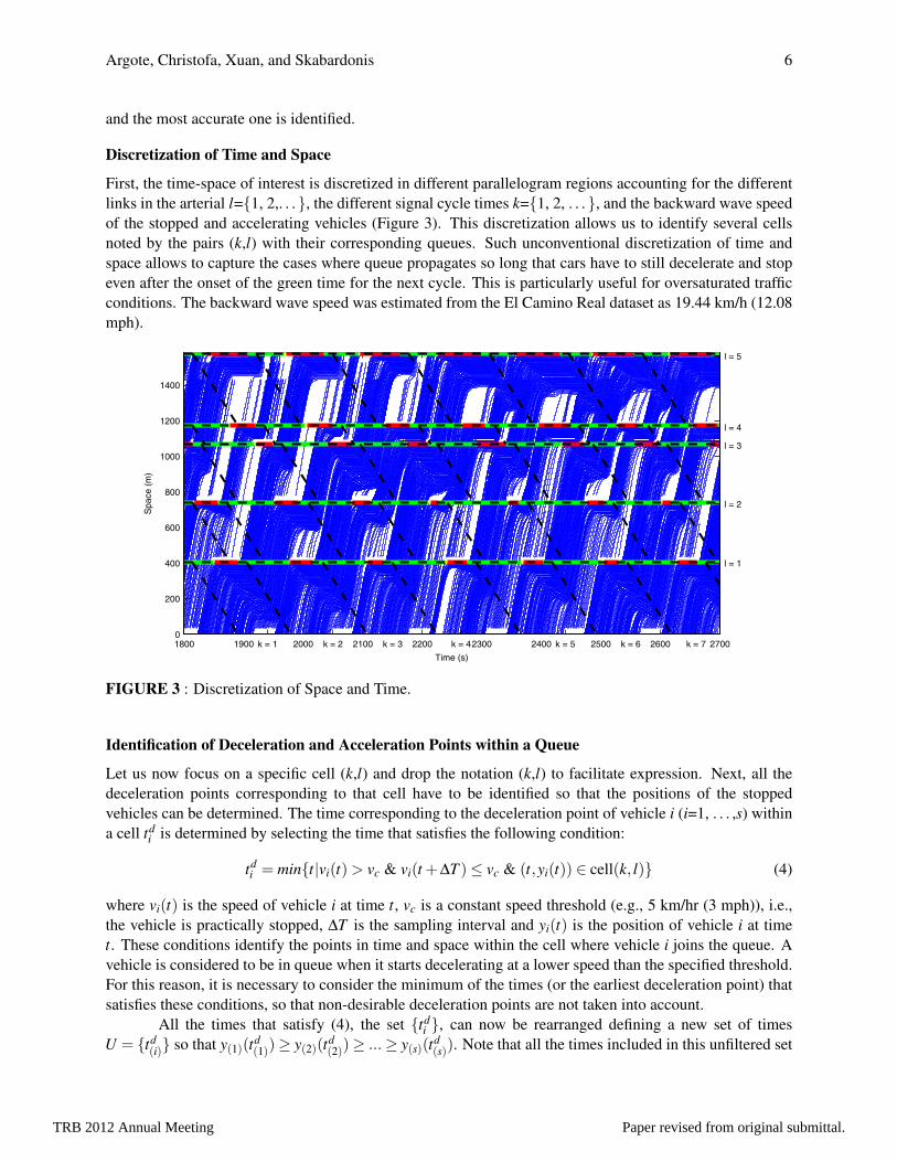
First, the time-space of interest is discretized in different parallelogram regions accounting for the differentlinks in the arterial l={1, 2,. . .}, the different signal cycle times k={1, 2, . . . }, and the backward wave speedof the stopped and accelerating vehicles (Figure 3). This discretization allows us to identify several cellsnoted by the pairs (k,l) with their corresponding queues. Such unconventional discretization of time andspace allows to capture the cases where queue propagates so long that cars have to still decelerate and stopeven after the onset of the green time for the next cycle. This is particularly useful for oversaturated trafficconditions. The backward wave speed was estimated from the El Camino Real dataset as 19.44 km/h (12.08mph).

1800 1900 2000 2100 2200 2300 2400 2500 2600 27000

200

400

600

800

1000

1200

1400

Time (s)

Spa

ce (

m)

k = 1 k = 2 k = 3 k = 4 k = 5 k = 6 k = 7

l = 1

l = 2

l = 3

l = 4

l = 5

FIGURE 3 : Discretization of Space and Time.

Identification of Deceleration and Acceleration Points within a Queue

Let us now focus on a specific cell (k,l) and drop the notation (k,l) to facilitate expression. Next, all thedeceleration points corresponding to that cell have to be identified so that the positions of the stoppedvehicles can be determined. The time corresponding to the deceleration point of vehicle i (i=1, . . . ,s) withina cell td

i is determined by selecting the time that satisfies the following condition:

tdi = min{t|vi(t)> vc & vi(t +∆T )≤ vc & (t,yi(t)) ∈ cell(k, l)} (4)

where vi(t) is the speed of vehicle i at time t, vc is a constant speed threshold (e.g., 5 km/hr (3 mph)), i.e.,the vehicle is practically stopped, ∆T is the sampling interval and yi(t) is the position of vehicle i at timet. These conditions identify the points in time and space within the cell where vehicle i joins the queue. Avehicle is considered to be in queue when it starts decelerating at a lower speed than the specified threshold.For this reason, it is necessary to consider the minimum of the times (or the earliest deceleration point) thatsatisfies these conditions, so that non-desirable deceleration points are not taken into account.

All the times that satisfy (4), the set {tdi }, can now be rearranged defining a new set of times

U = {td(i)} so that y(1)(td

(1))≥ y(2)(td(2))≥ ...≥ y(s)(td

(s)). Note that all the times included in this unfiltered set



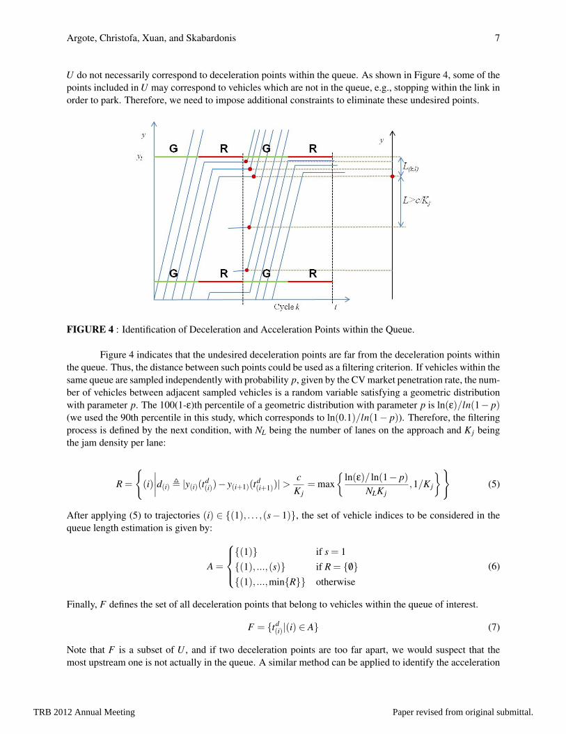
U do not necessarily correspond to deceleration points within the queue. As shown in Figure 4, some of thepoints included in U may correspond to vehicles which are not in the queue, e.g., stopping within the link inorder to park. Therefore, we need to impose additional constraints to eliminate these undesired points.

FIGURE 4 : Identification of Deceleration and Acceleration Points within the Queue.

Figure 4 indicates that the undesired deceleration points are far from the deceleration points withinthe queue. Thus, the distance between such points could be used as a filtering criterion. If vehicles within thesame queue are sampled independently with probability p, given by the CV market penetration rate, the num-ber of vehicles between adjacent sampled vehicles is a random variable satisfying a geometric distributionwith parameter p. The 100(1-ε)th percentile of a geometric distribution with parameter p is ln(ε)/ln(1− p)(we used the 90th percentile in this study, which corresponds to ln(0.1)/ln(1− p)). Therefore, the filteringprocess is defined by the next condition, with NL being the number of lanes on the approach and K j beingthe jam density per lane:

R =

{(i)∣∣∣∣d(i) , |y(i)(td

(i))− y(i+1)(td(i+1))|>

cK j

= max{

ln(ε)/ ln(1− p)NLK j

,1/K j

}}(5)

After applying (5) to trajectories (i) ∈ {(1), . . . ,(s− 1)}, the set of vehicle indices to be considered in thequeue length estimation is given by:

A =

{(1)} if s = 1{(1), ...,(s)} if R = { /0}{(1), ...,min{R}} otherwise

(6)

Finally, F defines the set of all deceleration points that belong to vehicles within the queue of interest.

F = {td(i)|(i) ∈ A} (7)

Note that F is a subset of U , and if two deceleration points are too far apart, we would suspect that themost upstream one is not actually in the queue. A similar method can be applied to identify the acceleration



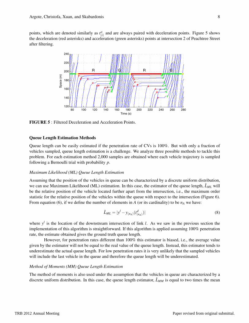
points, which are denoted similarly as ta(i) and are always paired with deceleration points. Figure 5 shows

the deceleration (red asterisks) and acceleration (green asterisks) points at intersection 2 of Peachtree Streetafter filtering.

80 100 120 140 160 180 200 220 240 260 280120

140

160

180

200

220

240

Time (s)

Spa

ce (

m)

R G GR

FIGURE 5 : Filtered Deceleration and Acceleration Points.

Queue Length Estimation Methods

Queue length can be easily estimated if the penetration rate of CVs is 100%. But with only a fraction ofvehicles sampled, queue length estimation is a challenge. We analyze three possible methods to tackle thisproblem. For each estimation method 2,000 samples are obtained where each vehicle trajectory is sampledfollowing a Bernoulli trial with probability p.

Maximum Likelihood (ML) Queue Length Estimation

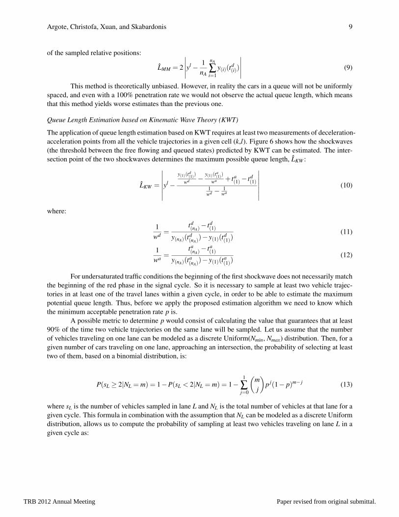
Assuming that the position of the vehicles in queue can be characterized by a discrete uniform distribution,we can use Maximum Likelihood (ML) estimation. In this case, the estimator of the queue length, L̂ML willbe the relative position of the vehicle located further apart from the intersection, i.e., the maximum orderstatistic for the relative position of the vehicles within the queue with respect to the intersection (Figure 6).From equation (6), if we define the number of elements in A (or its cardinality) to be nA we have:

L̂ML = |yl− y(nA)(td(nA)

)| (8)

where yl is the location of the downstream intersection of link l. As we saw in the previous section theimplementation of this algorithm is straightforward. If this algorithm is applied assuming 100% penetrationrate, the estimate obtained gives the ground truth queue length.

However, for penetration rates different than 100% this estimator is biased, i.e., the average valuegiven by the estimator will not be equal to the real value of the queue length. Instead, this estimator tends tounderestimate the actual queue length. For low penetration rates it is very unlikely that the sampled vehicleswill include the last vehicle in the queue and therefore the queue length will be underestimated.

Method of Moments (MM) Queue Length Estimation

The method of moments is also used under the assumption that the vehicles in queue are characterized by adiscrete uniform distribution. In this case, the queue length estimator, L̂MM is equal to two times the mean



of the sampled relative positions:

L̂MM = 2

∣∣∣∣∣yl− 1nA

nA

∑i=1

y(i)(td(i))

∣∣∣∣∣ (9)

This method is theoretically unbiased. However, in reality the cars in a queue will not be uniformlyspaced, and even with a 100% penetration rate we would not observe the actual queue length, which meansthat this method yields worse estimates than the previous one.

Queue Length Estimation based on Kinematic Wave Theory (KWT)

The application of queue length estimation based on KWT requires at least two measurements of deceleration-acceleration points from all the vehicle trajectories in a given cell (k,l). Figure 6 shows how the shockwaves(the threshold between the free flowing and queued states) predicted by KWT can be estimated. The inter-section point of the two shockwaves determines the maximum possible queue length, L̂KW :

L̂KW =

∣∣∣∣∣∣∣yl−y(1)(td

(1))

wd −y(1)(ta

(1))

wa + ta(1)− td

(1)1

wd − 1wa

∣∣∣∣∣∣∣ (10)

where:

1wd =

td(nA)− td

(1)

y(nA)(td(nA)

)− y(1)(td(1))

(11)

1wa =

ta(nA)− ta

(1)

y(nA)(ta(nA)

)− y(1)(ta(1))

(12)

For undersaturated traffic conditions the beginning of the first shockwave does not necessarily matchthe beginning of the red phase in the signal cycle. So it is necessary to sample at least two vehicle trajec-tories in at least one of the travel lanes within a given cycle, in order to be able to estimate the maximumpotential queue length. Thus, before we apply the proposed estimation algorithm we need to know whichthe minimum acceptable penetration rate p is.

A possible metric to determine p would consist of calculating the value that guarantees that at least90% of the time two vehicle trajectories on the same lane will be sampled. Let us assume that the numberof vehicles traveling on one lane can be modeled as a discrete Uniform(Nmin, Nmax) distribution. Then, for agiven number of cars traveling on one lane, approaching an intersection, the probability of selecting at leasttwo of them, based on a binomial distribution, is:

P(sL ≥ 2|NL = m) = 1−P(sL < 2|NL = m) = 1−1

∑j=0

(mj

)p j(1− p)m− j (13)

where sL is the number of vehicles sampled in lane L and NL is the total number of vehicles at that lane for agiven cycle. This formula in combination with the assumption that NL can be modeled as a discrete Uniformdistribution, allows us to compute the probability of sampling at least two vehicles traveling on lane L in agiven cycle as:



Time

Sp

ace

LML

LKW

^

^

(t ,y )(1) (1)

d d(t ,y )(1) (1)

a a

(t ,ya

(n ) (A

a

nA))(t ,y )d d

(n (nA A) )

G R G

Non-equiped veh

Equiped veh

FIGURE 6 : ML and KWT Queue Length Estimation.

P(sL ≥ 2) = 1−Nmax

∑m=Nmin

P(sL < 2|NL = m)P(NL = m) =

1− 1Nmax−Nmin +1

Nmax

∑m=Nmin

(1

∑j=0

(mj

)p j(1− p)m− j

)(14)

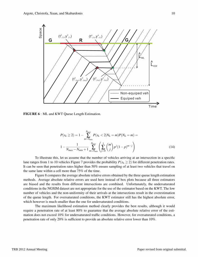
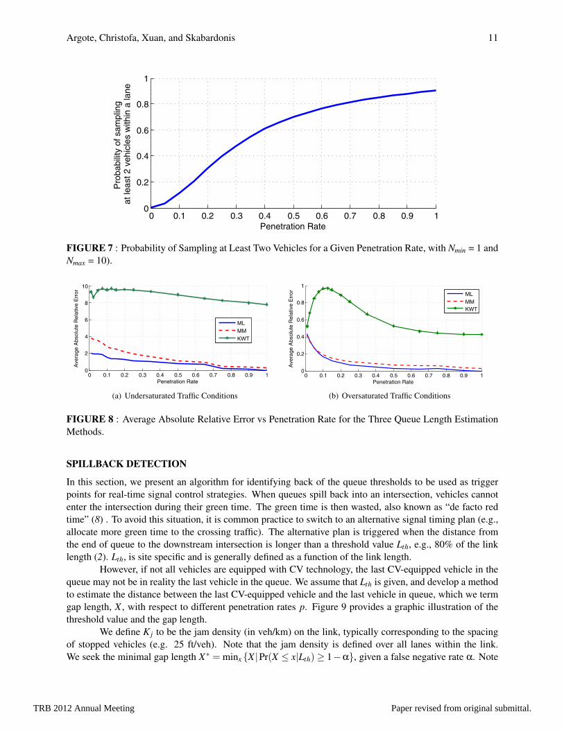
To illustrate this, let us assume that the number of vehicles arriving at an intersection in a specificlane ranges from 1 to 10 vehicles Figure 7 provides the probability P(sL ≥ 2) for different penetration rates.It can be seen that penetration rates higher than 50% ensure sampling of at least two vehicles that travel onthe same lane within a cell more than 75% of the time.

Figure 8 compares the average absolute relative errors obtained by the three queue length estimationmethods. Average absolute relative errors are used here instead of box plots because all three estimatorsare biased and the results from different intersections are combined. Unfortunately, the undersaturatedconditions in the NGSIM dataset are not appropriate for the use of the estimator based on the KWT. The lownumber of vehicles and the non-uniformity of their arrivals at the intersections result in the overestimationof the queue length. For oversaturated conditions, the KWT estimator still has the highest absolute error,which however is much smaller than the one for undersaturated conditions.

The maximum likelihood estimation method clearly provides the best results, although it wouldrequire a penetration rate of at least 80% to guarantee that the average absolute relative error of the esti-mation does not exceed 10% for undersaturated traffic conditions. However, for oversaturated conditions, apenetration rate of only 20% is sufficient to provide an absolute relative error lower than 10%.



0 0.1 0.2 0.3 0.4 0.5 0.6 0.7 0.8 0.9 10

0.2

0.4

0.6

0.8

1

Penetration Rate

Pro

babi

lity

of s

ampl

ing

at le

ast 2

veh

icle

s w

ithin

a la

ne

FIGURE 7 : Probability of Sampling at Least Two Vehicles for a Given Penetration Rate, with Nmin = 1 andNmax = 10).

0 0.1 0.2 0.3 0.4 0.5 0.6 0.7 0.8 0.9 10

2

4

6

8

10

Penetration Rate

Ave

rage

Abs

olut

e R

elat

ive

Err

or

MLMMKWT

(a) Undersaturated Traffic Conditions

0 0.1 0.2 0.3 0.4 0.5 0.6 0.7 0.8 0.9 10

0.2

0.4

0.6

0.8

1

Penetration Rate

Ave

rage

Abs

olut

e R

elat

ive

Err

or

MLMMKWT

(b) Oversaturated Traffic Conditions

FIGURE 8 : Average Absolute Relative Error vs Penetration Rate for the Three Queue Length EstimationMethods.

SPILLBACK DETECTION

In this section, we present an algorithm for identifying back of the queue thresholds to be used as triggerpoints for real-time signal control strategies. When queues spill back into an intersection, vehicles cannotenter the intersection during their green time. The green time is then wasted, also known as “de facto redtime” (8) . To avoid this situation, it is common practice to switch to an alternative signal timing plan (e.g.,allocate more green time to the crossing traffic). The alternative plan is triggered when the distance fromthe end of queue to the downstream intersection is longer than a threshold value Lth, e.g., 80% of the linklength (2). Lth, is site specific and is generally defined as a function of the link length.

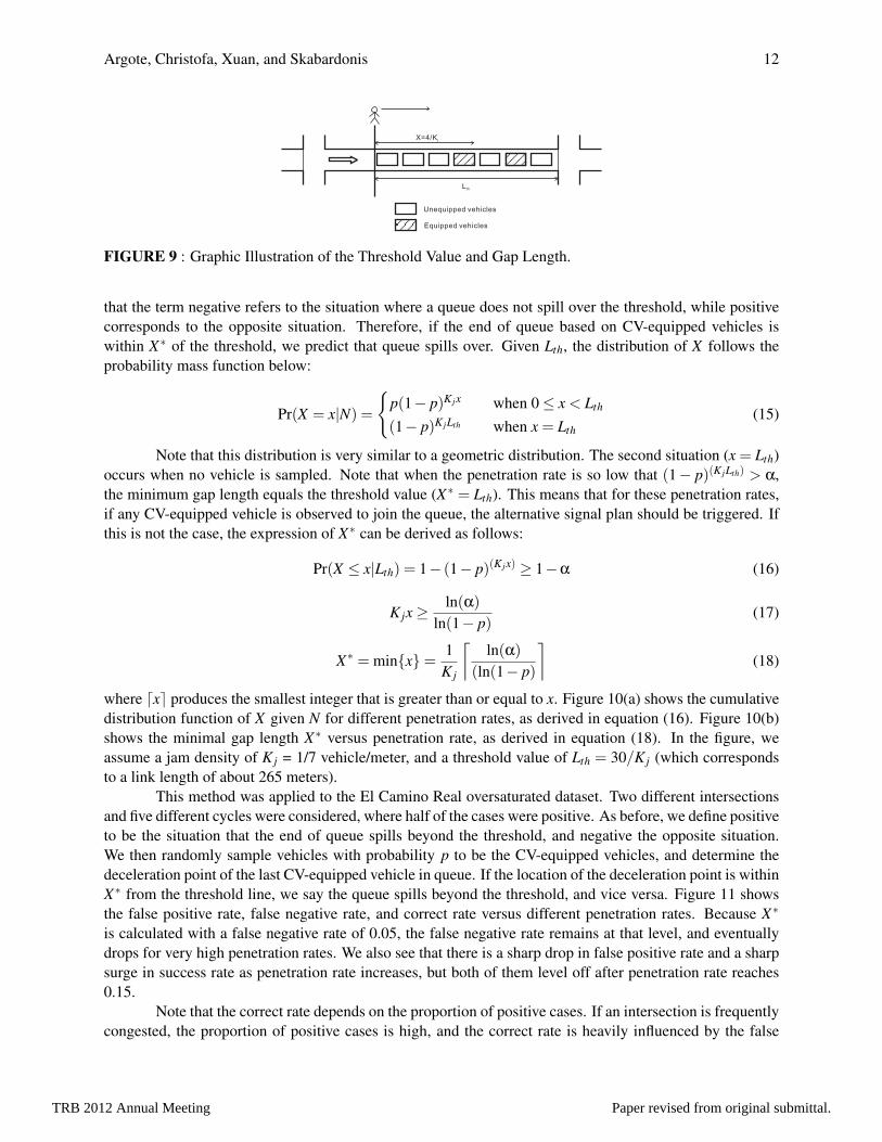
However, if not all vehicles are equipped with CV technology, the last CV-equipped vehicle in thequeue may not be in reality the last vehicle in the queue. We assume that Lth is given, and develop a methodto estimate the distance between the last CV-equipped vehicle and the last vehicle in queue, which we termgap length, X , with respect to different penetration rates p. Figure 9 provides a graphic illustration of thethreshold value and the gap length.

We define K j to be the jam density (in veh/km) on the link, typically corresponding to the spacingof stopped vehicles (e.g. 25 ft/veh). Note that the jam density is defined over all lanes within the link.We seek the minimal gap length X∗ = minx {X |Pr(X ≤ x|Lth)≥ 1−α}, given a false negative rate α. Note



Unequipped vehicles

Equipped vehicles

X=4/Kj

Lth

FIGURE 9 : Graphic Illustration of the Threshold Value and Gap Length.

that the term negative refers to the situation where a queue does not spill over the threshold, while positivecorresponds to the opposite situation. Therefore, if the end of queue based on CV-equipped vehicles iswithin X∗ of the threshold, we predict that queue spills over. Given Lth, the distribution of X follows theprobability mass function below:

Pr(X = x|N) =

{p(1− p)K jx when 0≤ x < Lth

(1− p)K jLth when x = Lth(15)

Note that this distribution is very similar to a geometric distribution. The second situation (x = Lth)occurs when no vehicle is sampled. Note that when the penetration rate is so low that (1− p)(K jLth) > α,the minimum gap length equals the threshold value (X∗ = Lth). This means that for these penetration rates,if any CV-equipped vehicle is observed to join the queue, the alternative signal plan should be triggered. Ifthis is not the case, the expression of X∗ can be derived as follows:

Pr(X ≤ x|Lth) = 1− (1− p)(K jx) ≥ 1−α (16)

K jx≥ln(α)

ln(1− p)(17)

X∗ = min{x}= 1K j

⌈ln(α)

(ln(1− p)

⌉(18)

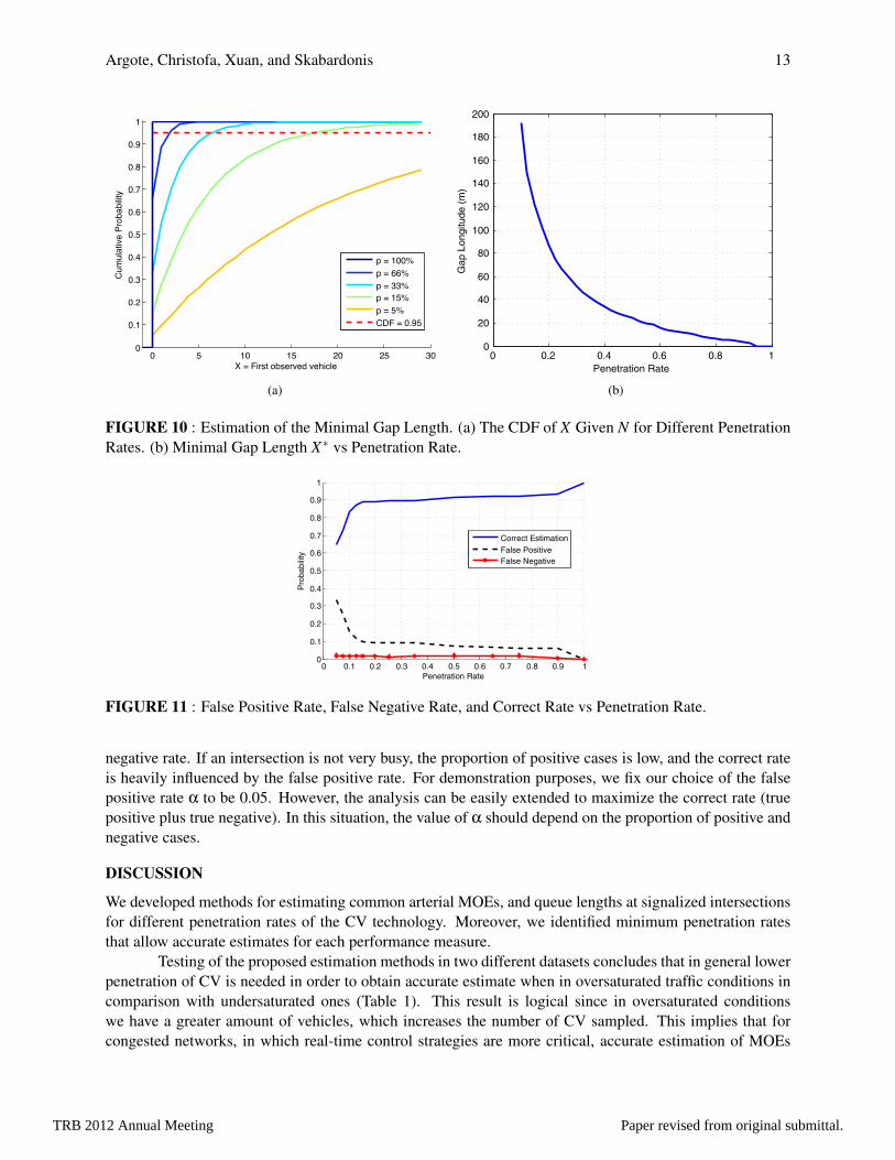
where dxe produces the smallest integer that is greater than or equal to x. Figure 10(a) shows the cumulativedistribution function of X given N for different penetration rates, as derived in equation (16). Figure 10(b)shows the minimal gap length X∗ versus penetration rate, as derived in equation (18). In the figure, weassume a jam density of K j = 1/7 vehicle/meter, and a threshold value of Lth = 30/K j (which correspondsto a link length of about 265 meters).

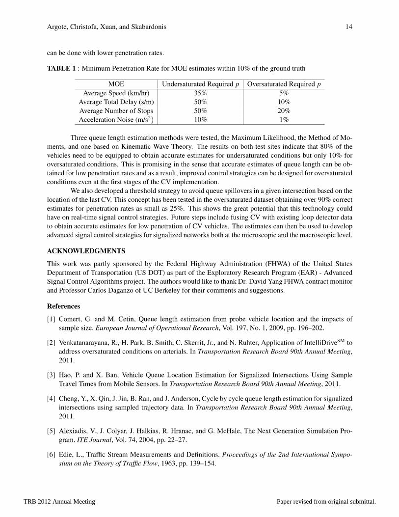
This method was applied to the El Camino Real oversaturated dataset. Two different intersectionsand five different cycles were considered, where half of the cases were positive. As before, we define positiveto be the situation that the end of queue spills beyond the threshold, and negative the opposite situation.We then randomly sample vehicles with probability p to be the CV-equipped vehicles, and determine thedeceleration point of the last CV-equipped vehicle in queue. If the location of the deceleration point is withinX∗ from the threshold line, we say the queue spills beyond the threshold, and vice versa. Figure 11 showsthe false positive rate, false negative rate, and correct rate versus different penetration rates. Because X∗

is calculated with a false negative rate of 0.05, the false negative rate remains at that level, and eventuallydrops for very high penetration rates. We also see that there is a sharp drop in false positive rate and a sharpsurge in success rate as penetration rate increases, but both of them level off after penetration rate reaches0.15.

Note that the correct rate depends on the proportion of positive cases. If an intersection is frequentlycongested, the proportion of positive cases is high, and the correct rate is heavily influenced by the false



0 5 10 15 20 25 300

0.1

0.2

0.3

0.4

0.5

0.6

0.7

0.8

0.9

1

X = First observed vehicle

Cum

ulat

ive

Prob

abilit

y

p = 100%p = 66%p = 33%p = 15%p = 5%CDF = 0.95

(a)

0 0.2 0.4 0.6 0.8 10

20

40

60

80

100

120

140

160

180

200

Penetration Rate

Gap

Lon

gitu

de (

m)

Student Version of MATLAB

(b)

FIGURE 10 : Estimation of the Minimal Gap Length. (a) The CDF of X Given N for Different PenetrationRates. (b) Minimal Gap Length X∗ vs Penetration Rate.

0 0.1 0.2 0.3 0.4 0.5 0.6 0.7 0.8 0.9 10

0.1

0.2

0.3

0.4

0.5

0.6

0.7

0.8

0.9

1

Penetration Rate

Pro

babi

lity

Correct EstimationFalse PositiveFalse Negative

FIGURE 11 : False Positive Rate, False Negative Rate, and Correct Rate vs Penetration Rate.

negative rate. If an intersection is not very busy, the proportion of positive cases is low, and the correct rateis heavily influenced by the false positive rate. For demonstration purposes, we fix our choice of the falsepositive rate α to be 0.05. However, the analysis can be easily extended to maximize the correct rate (truepositive plus true negative). In this situation, the value of α should depend on the proportion of positive andnegative cases.

DISCUSSION

We developed methods for estimating common arterial MOEs, and queue lengths at signalized intersectionsfor different penetration rates of the CV technology. Moreover, we identified minimum penetration ratesthat allow accurate estimates for each performance measure.

Testing of the proposed estimation methods in two different datasets concludes that in general lowerpenetration of CV is needed in order to obtain accurate estimate when in oversaturated traffic conditions incomparison with undersaturated ones (Table 1). This result is logical since in oversaturated conditionswe have a greater amount of vehicles, which increases the number of CV sampled. This implies that forcongested networks, in which real-time control strategies are more critical, accurate estimation of MOEs



can be done with lower penetration rates.

TABLE 1 : Minimum Penetration Rate for MOE estimates within 10% of the ground truth

MOE Undersaturated Required p Oversaturated Required pAverage Speed (km/hr) 35% 5%

Average Total Delay (s/m) 50% 10%Average Number of Stops 50% 20%Acceleration Noise (m/s2) 10% 1%

Three queue length estimation methods were tested, the Maximum Likelihood, the Method of Mo-ments, and one based on Kinematic Wave Theory. The results on both test sites indicate that 80% of thevehicles need to be equipped to obtain accurate estimates for undersaturated conditions but only 10% foroversaturated conditions. This is promising in the sense that accurate estimates of queue length can be ob-tained for low penetration rates and as a result, improved control strategies can be designed for oversaturatedconditions even at the first stages of the CV implementation.

We also developed a threshold strategy to avoid queue spillovers in a given intersection based on thelocation of the last CV. This concept has been tested in the oversaturated dataset obtaining over 90% correctestimates for penetration rates as small as 25%. This shows the great potential that this technology couldhave on real-time signal control strategies. Future steps include fusing CV with existing loop detector datato obtain accurate estimates for low penetration of CV vehicles. The estimates can then be used to developadvanced signal control strategies for signalized networks both at the microscopic and the macroscopic level.

ACKNOWLEDGMENTS

This work was partly sponsored by the Federal Highway Administration (FHWA) of the United StatesDepartment of Transportation (US DOT) as part of the Exploratory Research Program (EAR) - AdvancedSignal Control Algorithms project. The authors would like to thank Dr. David Yang FHWA contract monitorand Professor Carlos Daganzo of UC Berkeley for their comments and suggestions.

References

[1] Comert, G. and M. Cetin, Queue length estimation from probe vehicle location and the impacts ofsample size. European Journal of Operational Research, Vol. 197, No. 1, 2009, pp. 196–202.

[2] Venkatanarayana, R., H. Park, B. Smith, C. Skerrit, Jr., and N. Ruhter, Application of IntelliDriveSM toaddress oversaturated conditions on arterials. In Transportation Research Board 90th Annual Meeting,2011.

[3] Hao, P. and X. Ban, Vehicle Queue Location Estimation for Signalized Intersections Using SampleTravel Times from Mobile Sensors. In Transportation Research Board 90th Annual Meeting, 2011.

[4] Cheng, Y., X. Qin, J. Jin, B. Ran, and J. Anderson, Cycle by cycle queue length estimation for signalizedintersections using sampled trajectory data. In Transportation Research Board 90th Annual Meeting,2011.

[5] Alexiadis, V., J. Colyar, J. Halkias, R. Hranac, and G. McHale, The Next Generation Simulation Pro-gram. ITE Journal, Vol. 74, 2004, pp. 22–27.

[6] Edie, L., Traffic Stream Measurements and Definitions. Proceedings of the 2nd International Sympo-sium on the Theory of Traffic Flow, 1963, pp. 139–154.



[7] Jones, T. and R. Potts, The Measurement of Acceleration Noise-A Traffic Parameter. Operations Re-search, Vol. 10, No. 6, 1962, pp. 745–763.

[8] Abu-Lebdeh, G. and R. Benekohal, Development of traffic control and queue management proceduresfor oversaturated arterials. Transportation Research Record: Journal of the Transportation ResearchBoard, Vol. 1603, 1997, pp. 119–127.


Documents

Estimation of Arterial Measures of Effectiveness with ...xuanyg/doc/Argote_Christofa_Xuan... · Estimation of Arterial Measures of Effectiveness with Connected Vehicle Data ... the