I -

ESTIMATION OF ADSORPTION PARAMETERS FROM EXPERIMENTAL DATA

,

A REPORT SLJBMITTED TO

THE DEPARTMENT OF PETROLEUM ENGINEERING

OF STANFORD UNIVERSITY IN PARTIAL

FULFILLMENT OF THE REQUIREMENTS FOR

THE DEGREE OF MASTER OF SCIENCE

BY Ming Qi

May 1993

I certify that I have read this report and that in my opinion it is fully adequate, in scope and in quality, as partial fulfillment of the degree of Master of Science in Petroleum Engineering.

~

, I

c

A tu.& (Principal Advisor)

Contents

1 Introduction 1

2 Previous Work 6

3 Experiment Apparatus and Procedures 10

3.1 Apparatus . . . . . . . . . . . . . . . . . . . . . . . . . . . . . . . . . 10

3.2 Samples Used in the Experiments by Michael Harr . . . . . . . . . . 11

3.3 Samples Used in the Present Experiment . . . . . . . . . . . . . . . . 11

3.4 Procedures 12

3.4.1 Experiment Procedures . . . . . . . . . . . . . . . . . . . . . . 12

3.4.2 Parameter Estimation Procedures . . . . . . . . . . . . . . . . 13

. . . . . . . . . . . . . . . . . . . . . . . . . . . . . . . . .

4 Results and Discussions 15

4.1 Experimental Results . . . . . . . . . . . . . . . . . . . . . . . . . . . 15

4.2 Comparison of the Results . . . . . . . . . . . . . . . . . . . . . . . . 15

4.3 Effect of Permeability . . . . . . . . . . . . . . . . . . . . . . . . . . . 17

4.4 Effect of Porosity . . . . . . . . . . . . . . . . . . . . . . . . . . . . . 17

5 Conclusions and Recommendations 31 5.1 Conclusions . . . . . . . . . . . . . . . . . . . . . . . . . . . . . . . . 31

5.2 Recommendations . . . . . . . . . . . . . . . . . . . . . . . . . . . . . 32

6 Nomenclature 33

7l Bibliography

~

1

34

CONTENTS

8 Appendix

.. 11

37 I

List of Tables

1 Classification of pores according to IUPAC(1972) . . . . . . . . . . . 2 ~

2 Rock Samples Used by Michael Harr . . . . . . . . . . . . . . . . . . 11

3 Rock Samples Used in Pressure Transient Experiment . . . . . . . . . 12 ~

... 111

List of Figures

3.1 Schematic Diagram of Experimental System Setup . . . . . . . . . . . 14

4.1 Pressure Transient Experiment Result . Geysers Shallow Reservoir . . 4.2 Pressure Transient Experiment Result . Geysers Geothermal Field . . 4.3 Pressure Transient Experiment Result . Geysers Geothermal Field . .

4.4 Pressure Transient Experiment Result . Montiverdi, Italy . . . . . . . 4.5 Pressure Transient Experiment Result . Reykjanes, Iceland . . . . . . 4.6 Pressure Transient Experiment Result . Geysers Geothermal Field . . 4.7 Pressure Transient Experiment Result . Geysers Geothermal Field . . 4.8 Pressure Transient Experiment Result . Reykjanes, Iceland . . . . . . 4.9 Geysers Unknown Well, Depth 5000 . 5200 Feet, 28-150 Mesh . . . . 4.10 Geysers Well OF52.11, Depth 5000 . 5200 Feet, 10-150 Mesh . . . . . 4.11 Geysers Well OF52.11, Depth 5000 . 5200 Feet, 20-150 Mesh . . . . . 4.12 Montiverdi Well No.2, 10-150 Mesh . . . . . . . . . . . . . . . . . . . 4.13 Reykjanes Well No.9, 10- 100 Mesh . . . . . . . . . . . . . . . . . . . 4.14 Geysers Well Megu-15 ST2, Depth 8600 . 8800 Feet, 20-150 Mesh . . 4.15 Geysers Well OF52.11, Depth 8000 . 8200 Feet, 30-80 Mesh . . . . . 4.16 Geysers Well OF52.11, Depth 8000 . 8200 Feet, 30-150 Mesh . . . . . 4.17 Compare of the Experiment Results . Reykjanes Well 9 . . . . . . . . 4.18 Compare of the Experiment Results . Geysers Unknown Well . . . . . 4.19 Compare of the Experiment Results . Geysers Well OF52-11 . . . . . 4.20 Isotherms from Different Experiments . Montiverdi 2 . . . . . . . . . 4.21 Effect of Different Permeability . Geysers Unknown Well . . . . . . . 4.22 Effect of Different Permeability . Geysers Well OF52-11 . . . . . . . .

18

18

19

19

20

20

21

21

22

22

23

23

24

24

25

25

26

26

27

27

28

28

iv

LIST OF FIGURES V I

4.23 Effect of Different Permeability . Well Montiverdi 2 . . . . . . . . . . 2 9 1

4.24 Effect of Different Porosity . Geysers Unknown Well . . . . . . . . . . 29 I

4.26 Effect of Different Porosity . Well Montiverdi 2 . . . . . . . . . . . . 30 4.25 Effect of Different Porosity . Geysers Well OF52-11 . . . . . . . . . . 30

Abstract

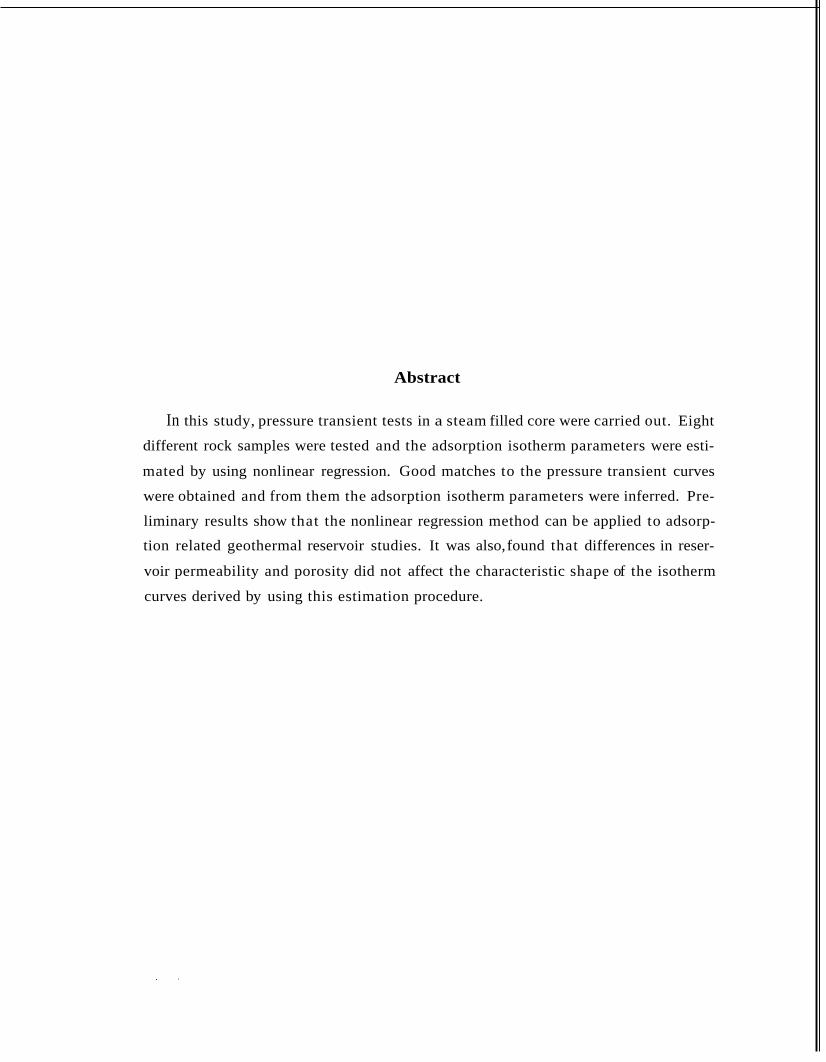
In this study, pressure transient tests in a steam filled core were carried out. Eight

different rock samples were tested and the adsorption isotherm parameters were esti-

mated by using nonlinear regression. Good matches to the pressure transient curves

were obtained and from them the adsorption isotherm parameters were inferred. Pre-

liminary results show that the nonlinear regression method can be applied to adsorp-

tion related geothermal reservoir studies. It was also, found that differences in reser-

voir permeability and porosity did not affect the characteristic shape of the isotherm

curves derived by using this estimation procedure.

Chapter 1

Introduction

When a gas or vapor is brought i n contact with an evacuated solid, a part of it may

be taken up by the solid. If this occurs at constant volume, the pressure drops; if

at constant pressure, the volume decreases. The molecules that disappear from the

gas phase either enter the inside of the solid, or remain on the outside, attached to

its surface. The former phenon~enon is called absorption; the latter adsorption. The

solid that takes up the gas or vapor is called the adsorbent, the gas or vapor attached

t p the surface of the solid is called the adsorbate. Often the two occur simultaneously,

the total uptake of the gas is then designated by the term sorption.

There are two types of adsorption exist: physical, adsorption (physisorption) and

chemical adsorption (chemisorption). Physisorption involves intermolecular forces

(van de Waals forces, hydrogen bonds, etc.) whereas chemisorption is connected with the formation of a chemical compound involving the adsorbent and the primary layer

of the substance adsorbed. Steam adsorption on the solid is considered as physical

adsorption.

The phenomenon of adsorption has long been known. As early as in 1777 Fontana

(1777) had noted that freshly calcined charcoal, cooled under mercury, was able to

take up several times its own volume of various gases; and in the same year Scheele

(1777) recorded that air expelled from charcoal on heating was taken up again on

cooling. It was soon realized that the volume taken up varies from one charcoal to

another and from one gas to another. In suggesting that the efficiency of the solid

depended 011 the area of exposed surface, de Saussure (1814) anticipated our present-

day views 011 the subject. Mitscherlich (1843), on the other hand, emphasized the

role of the pores in charcoal, and estimated their average diameter to be 1/2400 in;

it would seem that carbon dioxide condensed into layers 0.005 mm thick in a form

closely resembling liquid carbon dioxide. These two factors, surface area and porosity

(or pore volume), are now recognized to play complementary parts in adsorption

phenomena, not only in charcoal but in a vast range of other solids. It thus comes

about that measurements of adsorption of gases or vapors can be made to yield

information as to the surface area and the pore structure of the solid.

The pore systems of solids are of many different kinds. The individual pores may

vary greatly both in size and in shape within a given solid, and between one solid and

another. A feature of special interest for many purposes is the “width w” of the pores,

e.g. the diameter of a cylindrical pore, or the distance between the sides of a slit-

shaped pore. According to the International Union of Pure and Applied Chemistry

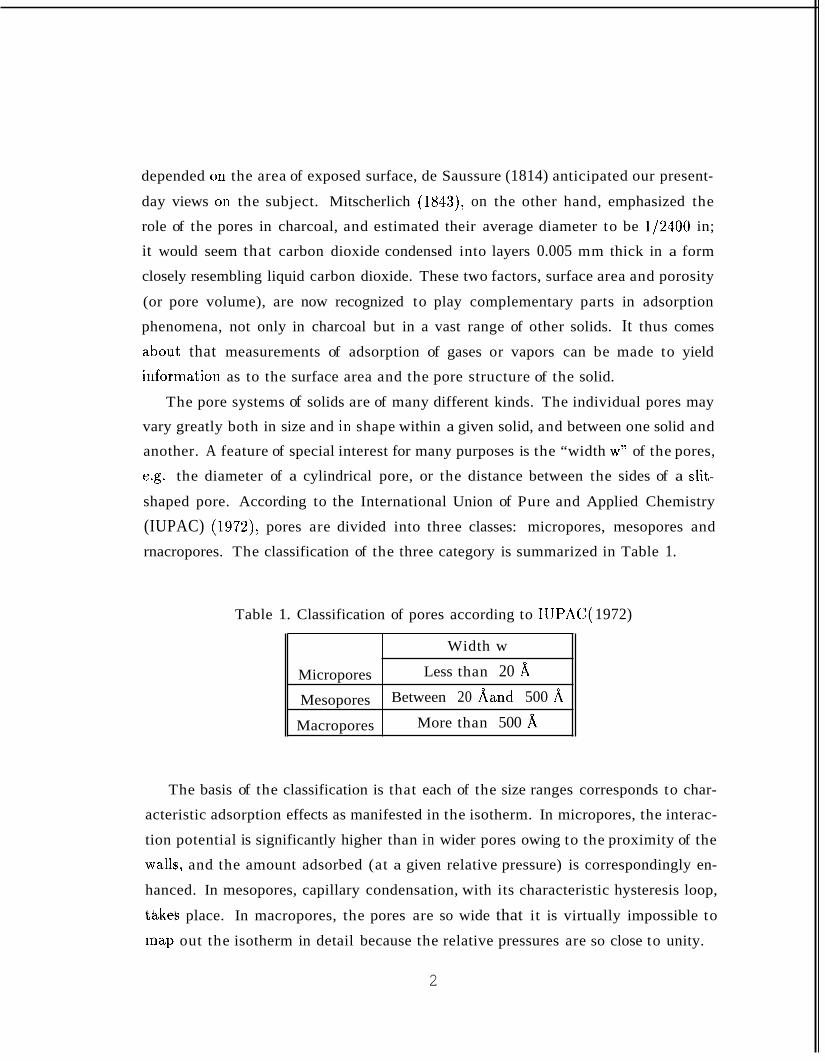
(IUPAC) (1972), pores are divided into three classes: micropores, mesopores and

rnacropores. The classification of the three category is summarized in Table 1.

Table 1. Classification of pores according to IUPAC( 1972)

Width w

Micropores

More than 500 A Macropores

Between 20 Aand 500 8, Mesopores

Less than 20 8,

The basis of the classification is that each of the size ranges corresponds to char-

acteristic adsorption effects as manifested in the isotherm. In micropores, the interac-

tion potential is significantly higher than in wider pores owing to the proximity of the

walls, and the amount adsorbed (at a given relative pressure) is correspondingly en-

hanced. In mesopores, capillary condensation, with its characteristic hysteresis loop,

takes place. In macropores, the pores are so wide that it is virtually impossible to

npap out the isotherm in detail because the relative pressures are so close to unity. 1 1

2

For a given gas or vapor and unit weight of a given adsorbent the amount of gas

or vapor adsorbed at equilibrium is a function of the final pressure and temperature

only,

a = f ( P , T ) (1.1)

where a is the amount adsorbed per gram of adsorbent, p in the equilibrium pressure,

and T is the absolute temperature. Usually either the pressure or the temperature

alone is varied, while the other is kept constant. When the pressure of the gas or

vapor is varied and the temperature is kept constant, the plot of the amount adsorbed

against the pressure is called the adsorption isotherm, and the isotherm equation is:

a = f ( p ) T = constant (1 4 When the temperature is varied and the pressure is kept constant, one obtains

the adsorption isobar:

a = f ( T ) p = constant (1-3)

The adsorption isotherm is the most widely used in the field of adsorption. In

studying the adsorption/desorption phenomenon associated with vapor-dominated

geothermal reservoirs, we use the adsorption/desorption isotherm with the unit of

gram of water adsorbed per gram of solid (gram water adsorbed)/(gram solid).

Vapor-dominated geothermal reservoirs occur when the fluid pressure in the pro-

ducing zone is at or below the saturation pressure corresponding to the reservoir

temperature. Only a few geothermal fields in the world satisfy this criterion. These

include the Geysers field in northern California and the Larderello field in Italy. Al- though they are few in number, the vapor-dominated geothermal reservoirs offer the

most readily used form of geothermal fluid, namely high enthalpy, used to power

turbines for the generation of electricity.

Studies of reservoir and production behavior of vapor-dominated geothermal sys-

tem have focused on estimates of resource size, reservoir longevity and resource man-

agement. Traditionally, it has been considered that superheated steam and rock are I

3

the only two components i n a dry steam geothermal reservoir like the Geysers. From

the fundamental physical properties of fluid and rock, however, there should exist a

certain amount of liquid in addition of steam. However the reservoir pressure at the

Geysers is too low for water to exist in the form of bulk liquid at the reservoir temper-

ature. It has been proposed thak water might exist as adsorbed liquid in micropores

(White, 1973; Hsieh, 1980). Evidence from both laboratory' studies and field data

indicates that storage of liquid as micropore fluid is likely (Hsieh, 1980; Hsieh and

Rarney, 1983; Nghiem and Ramey, 1990).

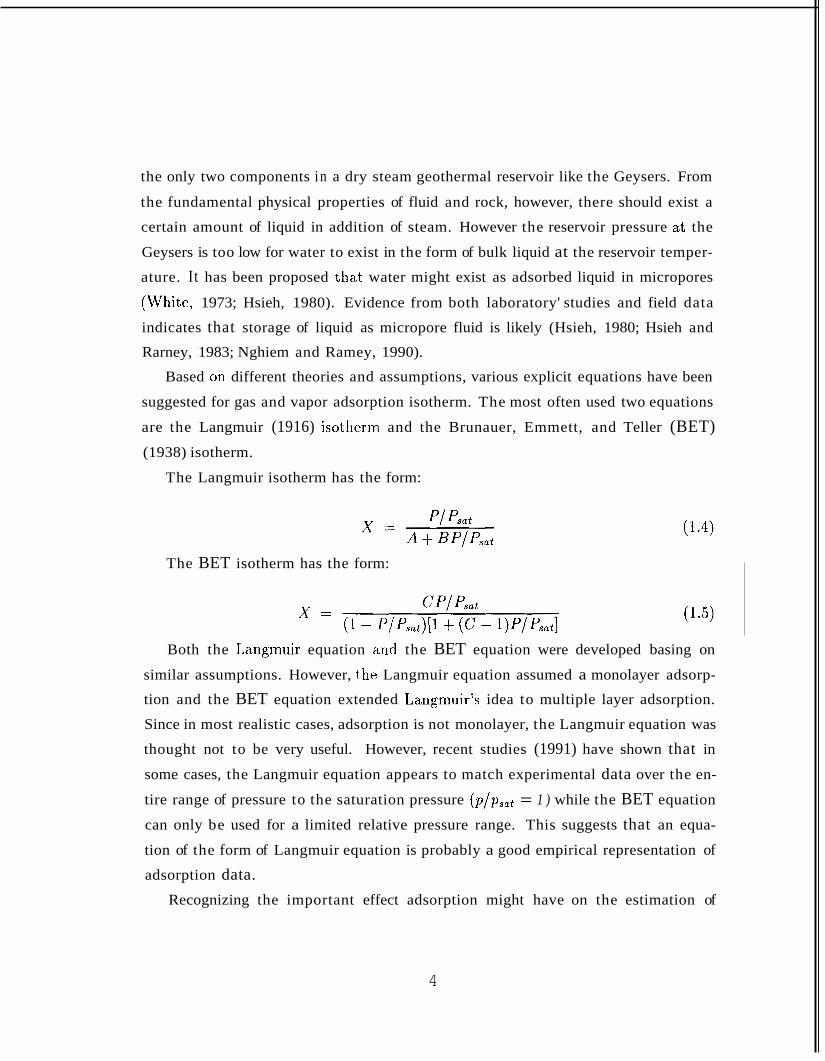
Based on different theories and assumptions, various explicit equations have been

suggested for gas and vapor adsorption isotherm. The most often used two equations

are the Langmuir (1916) isot11t:rm and the Brunauer, Emmett, and Teller (BET) (1938) isotherm.

The Langmuir isotherm has the form:

The BET isotherm has the form:

Both the Laugmuir equation and the BET equation were developed basing on

similar assumptions. However, t'he Langmuir equation assumed a monolayer adsorp-

tion and the BET equation extended Langmuir's idea to multiple layer adsorption.

Since in most realistic cases, adsorption is not monolayer, the Langmuir equation was

thought not to be very useful. However, recent studies (1991) have shown that in

some cases, the Langmuir equation appears to match experimental data over the en-

tire range of pressure to the saturation pressure (PIPsat = 1 ) while the BET equation

can only be used for a limited relative pressure range. This suggests that an equa-

tion of the form of Langmuir equation is probably a good empirical representation of

adsorption data. Recognizing the important effect adsorption might have on the estimation of

4

geothernlal reservoir performance, several models which considered the effects of ad-

sorption have been developed and tested by different authors (Moench and Atkinson,

1978; Herkelrath, Moench and O’Neal, 1983). The most recent model was devel-

oped by Nghiem and Ramey (1990) and a simulator was developed to simulate the

one-dimensional steam flow i n a, homogeneous porous media. Surprisingly, by fitting

the experimental isotherm.data, they found that the Langmuir isotherm could match

several measured data over the entire relative pressure range to P/P,,, = 1 while the

BET isotherm did not. By using the Langmuir isotherm, Nghiem and Ramey (1990)

simulated one-dimensional flow in a geothermal reservoir and predicted the pressure

change of the reservoir under specified production conditions.

To use the Langmuir isotherm (Eqn. 1.4), two coefficients have to be specified.

Nghiem and Ramey determined them by fitting certain experimental data. However

the adsorption isotherm is different from one system to another. For each system, a set

of coefficients needs to be determined. Herkelrath et al. (1983) studied the transient

flow of pure steam in a unifornl porous medium and found that the time required for

steam pressure transients to propagate through an unconsolidated material containing

sand, silt, and clay was 10-25 times longer than predicted by conventional superheated

steam flow theory. They concluded that the delay in the steam pressure breakthrough

was caused by adsorption of steam i n the porous sample. This originated the idea of

estimating of adsorption parameters from pressure transient experiments.

In this study, a number of steam pressure transient experiments were carried

out. Nghiem and Ramey’s (1991 ) simulator was run in combination with a nonlinear

regression program to simulate the precess. The steam pressure transient results

are believed to reflect the affect of adsorption. By fitting the experimental pressure

transient data, the Langmuir isotherm parameters can be extracted by using nonlinear

regression.

Chapter 2

Previous Work

In 1980, Hsieh (1980) studied the vapor pressure lowering phenomenon in porous

media and measured the adsorption/desorption isotherms of water vapor, methane,

and ethane with several different core samples. The experiment proved that the water

vapor pressure lowering in rock is dominated by micropore adsorption and Hsieh

(1980) suggested that the adsorbed water may be an important source of steam in

vapor dominated geothermal systems. Although Hsieh (1980) concluded that there

were no significant hysteresis loops in water adsorption/desorption isotherm, some of

his results did show visible differences between adsorption and desorption isotherms.

In 1983, Herkelrath, Moench, and O’Neal conducted laboratory investigations of

steam flow in a porous mediunl. They ran the transient, superheated steam flow

experiments by bringing a cylinder of porous material to a uniform initial pressure

and then making a step increase in pressure at one end of the sample while monitoring

the pressure transient breakthrough at the other end. They found the breakthrough

time for steam pressure was 10--25 times longer than predicted by conventional (no

adsorption) superheated steam flow theory. A new model including the effect of

adsorption was developed and tested by using it to simulate the experimental pressure

transient process. They assumed the steam pressure was a function of temperature

and the amount of water adsorption:

6

where Po(?") represented the saturated vapor pressure function, and R(S) was the

relative vapor pressure, which was a function of the fraction of the pore space that

was filled with adsorbed water. To find out the function R(S), adsorption isotherm

data were needed. So Herkelrath et a1 (1983) had to run additional tests similar

to the those run by Hsieh and Ramey (1983) to measure the adsorption isotherm

at equilibrium. Then by fitting the isotherm data with an empirical relation they

obtained a function for R(S) of the following form:

R( ,?) = A( 10-[lO(B-s)C1) (2.2)

where A, B, and C were const'ants determined by least squares fitting (A= 1.078,

B=0.00821, C=0.0224 in their case). The results of the simulation were compared

to the experimental data and good agreement between simulation and experimental

results was achieved.

Economides and Miller (1985) also studied the effects of the adsorption phenom-

ena in the evaluation of vapor-dominated geothermal reservoirs. In their study, the

conventional models for material balance and pressure transient behavior were ex-

tended to incorporate the effects of adsorption. Again an adsorption isotherm was

needed for calculation. They used a simple linear equation of the following form to

calculate the isotherm approximately:

where X is the amount absorbed, a is an experimental constant, p is the pressure and

p" is the saturated vapor pressure.

To do the calculation, 'the constant cr needs to be determined first. Economides

and Miller (1985) used the constants obtained from the experiments by Hsieh (1980). Nghiem and Ranley (1991) developed another model including adsorption to

simulate a one-dimensional vapor dominated geothermal reservoir. The Langmuir

isotherm (Eqn. 1.4) was used and the two constants in the equation (A and B) were

determined from the experimental data from Herkelrath and O'Neal (1985), and from

Herkelrath (1990). Then, performance forecasting for a hypothetical field with the

7

Geysers greywacke rock was performed to demonstrate the importance of the desorp-

tion. The results of Nghiem and Ramey also support the theory that adsorption is

the dominant mechanism for steam storage in geothermal reservoir.

Michael Harr (1991) also measured the adsorption/desorption of steam in porous

media in the laboratory. He ran a series of equilibrium measurements of the steam

adsorption and desorption isotllerms by using a sorptometer. Different geothermal

field rocks were tested at different temperatures and the results were compared. Harr

found that the adsorption and desorption isotherms measured at different temperature

were different. Also there was a large hysteresis between adsorption and desorption.

Harr also ran a pressure transient test using the equipment borrowed from USGS (the

same equipment used by Herkrlrath et a1 in 1983). Four pressure transient curves

were obtained. A large hysteresis between adsorption and desorption was observed.

All previous work strongly s'upports the theory that adsorption is the dominant

reservoir storage mechanism in vapor-dominated geothermal reservoir and by includ-

ing the effect of adsorption we can make better forecasts of the reservoir performance.

One difficulty in doing this is tha,t we require measured adsorption isotherm data. The

measurement of adsorption isot,herms in the laboratory requires specially designed

equipment and is usually very time consumming. Another difficulty is that the steam

adsorption isotherms are quite different from one rock to another. Therefore, the ad-

sorption isotherm obtained from one rock sample can not be used for another. This

restricts the usage of the simuhtors and thus makes their results less general.

Some of the previous works (Herklrath et al., 1983; Harr, 1991) also demonstrated

that adsorption had a great effect on the pressure transient. By analyzing the pressure

transient curves we might be a b k to infer the adsorption isotherm. This will eliminate

the necessity of adsorption isotherm measurement and finally enable us to estimate

the isotherm from field pressure decline curve. After all, the field pressure decline

curve is usually available for most geothermal fields.

In this study, Michael Harr's vapor pressure transient experiment was cont,in-

ued, by using the same experiment equipment with some modification of the data

acquisition system. More pressure transient data are made available. A computer

8

program is developed combining the nonlinear regression and a one-dimensional sim-

ulator (Nghiem and Ramey, 1991). The method of estimating adsorption the isotherm

from pressure transient curve i s tested. Some of the estimated isotherm results are

compared with the isotherm data obtained by Shang (1992) in equilibrium experi-

ments.

9

Chapter 3

Experiment Apparatus and

Procedures

3.1 Apparatus

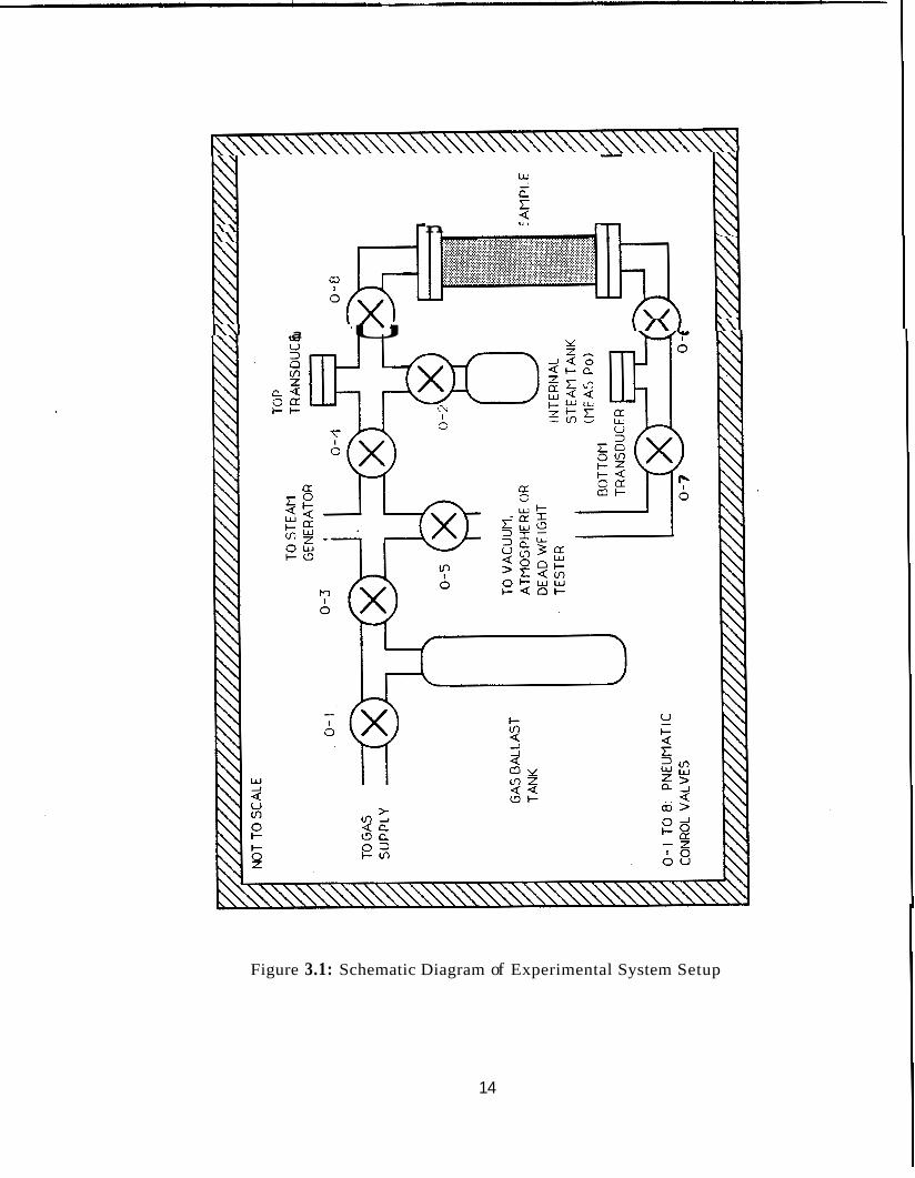
The equipment used was built originally by Herkelrath et al. (1983) at the U.S.G.S. It is the same equipment that l\ilic,hael Harr (1991) used in his experiment. Figure

3.1 shows a schematic diagram of the setup.

The equipment consists of four major parts: steam generator, air bath, vacuum

system, and data recording system. The steam generator produces steam at a, set

temperature for the duration of the experiment. The air bath is used to maintain a

constant temperature during the experiment, the vacuum system is used to outgas the

sample before the transient run and evacuate the connecting tubes for pressure mea-

surements. The data acquisition system used before in the transient test equipment

was an old-fashioned Digital RX02 computer with a VT105 monitor. The pressure

transient data were first recorded on 8 inch floppy diskette. Then the diskette needed

to be taken to the U.S.G.S. to have the data transferred from the diskette onto an

IBM-PC or a Macintosh diskette for further use. This was very inconvenient. In this

study, we successfully replaced the old monitor with an IBM-PC computer so that

the pressure transient data can be seen and saved directly onto the IBM-PC. There is

asdetailed description and explanation about the structure and function of each part

10

of the equipment in Appendix A of Michael Harr’s report (Harr, 1991).

3.2 Samples Used. in the Experiments by Michael

Harr

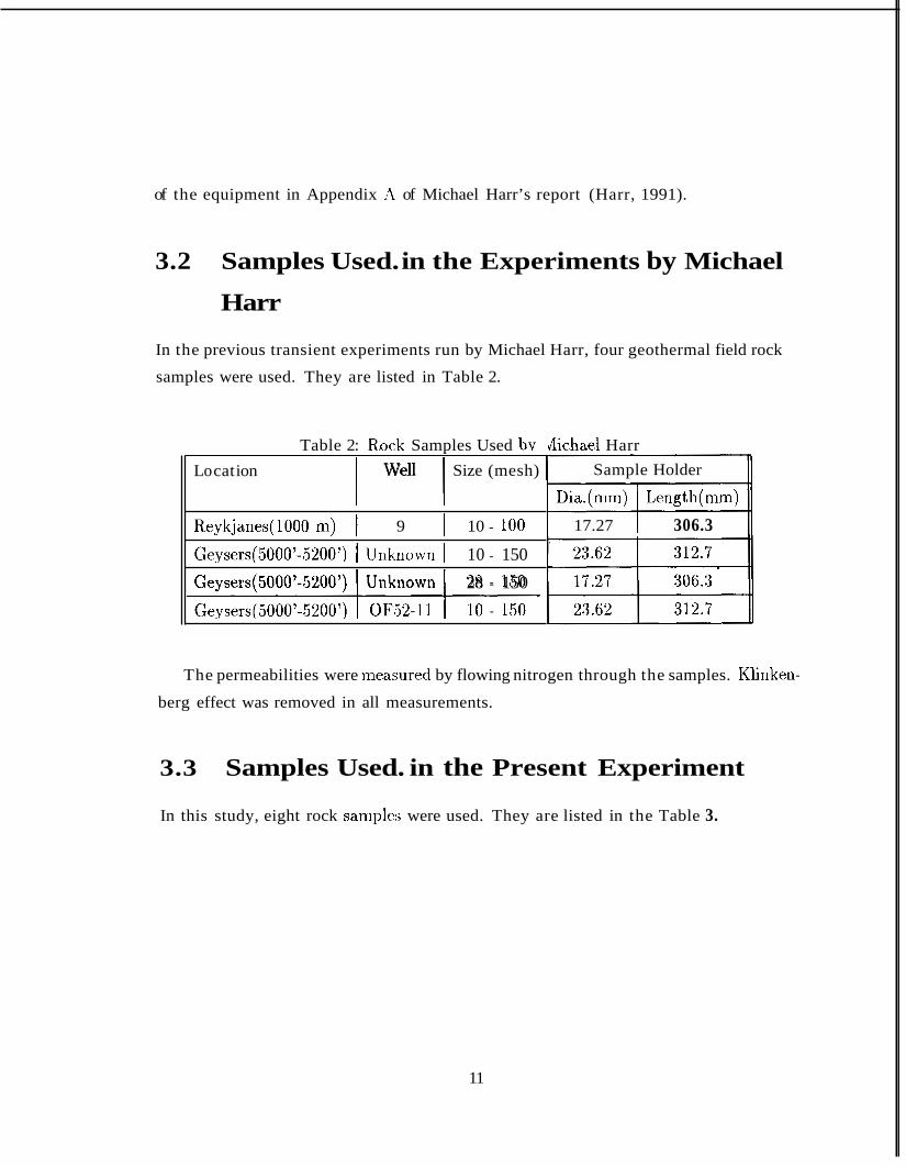
In the previous transient experiments run by Michael Harr, four geothermal field rock

samples were used. They are listed in Table 2.

Table 2: Roc,k Samples Used bv Lo cat ion I I Well Size (mesh)

Reykjanes(1000 In) I 9 I 10 - 100

Geysers(5000’-5200’) I Unk:nown I 10 - 150

-d* Geysers(5000’-5200’) Unkxown 28 - 150

dichael Harr Sample Holder

Dia.(mm) I Length(mm)

17.27 I 306.3

The permeabilities were measured by flowing nitrogen through the samples. Klinken-

berg effect was removed in all measurements.

3.3 Samples Used. in the Present Experiment

In this study, eight rock samples were used. They are listed in the Table 3.

11

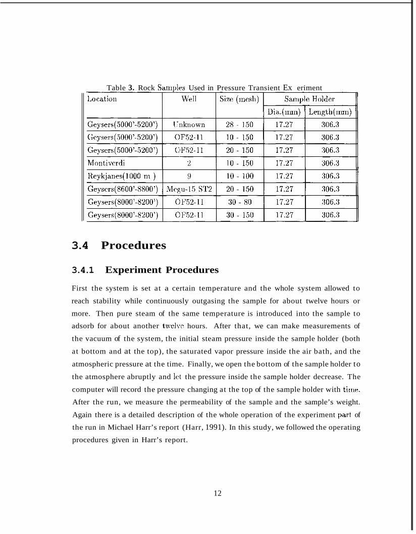
Table 3. Rock Sampl’es Used in Pressure Transient Ex eriment

3.4 Procedures

3.4.1 Experiment Procedures

First the system is set at a certain temperature and the whole system allowed to

reach stability while continuously outgasing the sample for about twelve hours or

more. Then pure steam of the same temperature is introduced into the sample to

adsorb for about another twelvle hours. After that, we can make measurements of

the vacuum of the system, the initial steam pressure inside the sample holder (both

at bottom and at the top), the saturated vapor pressure inside the air bath, and the

atmospheric pressure at the time. Finally, we open the bottom of the sample holder to

the atmosphere abruptly and let, the pressure inside the sample holder decrease. The

computer will record the pressure changing at the top of the sample holder with time.

After the run, we measure the permeability of the sample and the sample’s weight.

Again there is a detailed description of the whole operation of the experiment part) of

the run in Michael Harr’s report (Harr, 1991). In this study, we followed the operating

procedures given in Harr’s report.

12

3.4.2 Parameter Estimation Procedures

With the data measured as above, we can run our program to obtain estimated ad-

sorption parameters. The progam uses the one-dimensional steam flow simulator

‘Adsorption’ as a subroutine to1 simulate the transient experiment. With a pair of

guessed parameters of A and H, the subroutine ‘Adsorption’ calculates the transient

steam pressure. This simulated result is then compared with experimental result. If they are different, nonlinear regression is employed by calling subroutine ‘dumpol’.

The subroutine ‘dumpol’ uses the polytope algorithm to minimize the difference be-

tween simulated and experimental results. At each iteration, a new set of A and H is

generated to replace the old one and is used to run the subroutine ‘Adsorption’ again.

This procedure repeated until a. good match between simulated and experimental re-

sults is achieved. A list of the program is included in the appendix. For more detail

about the subroutine ‘dumpol’ please see User’s Manual of FORTRAN Subroutines

for Mathematical Applications (IMSL).

13

n n

a U

Figure 3.1: Schematic Diagram of Experimental System Setup

14

Chapter 4

Results and Discussio.ns

4.1 Experimental Results

All runs are under the same temperature conditions that Michael Harr used in his

runs( 125 “C) so that we could compare some of our data with Michael Harr’s data for

the purpose of checking and analyzing. No higher temperature were used i n the fear

that excessive heating would cause the O-rings in the pneumatic valves located inside

the oven to acquire a permanent set and thus cause the leakage problems as noted

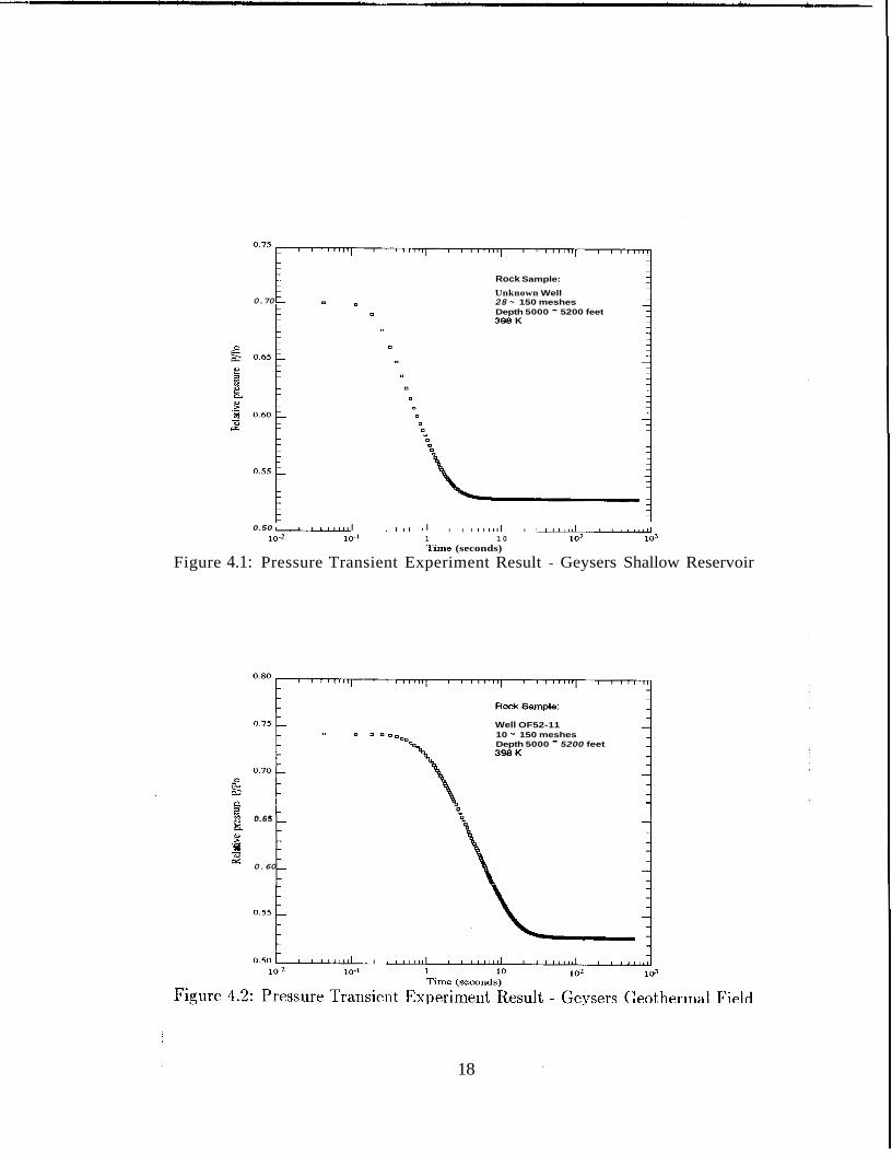
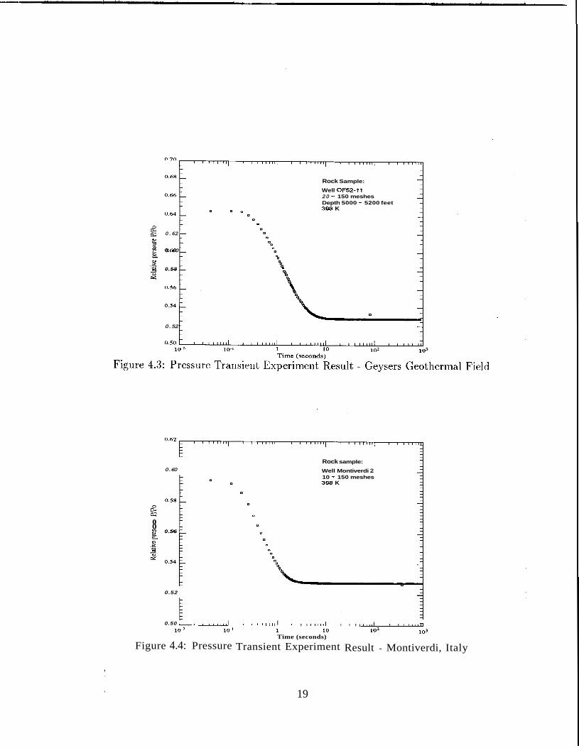
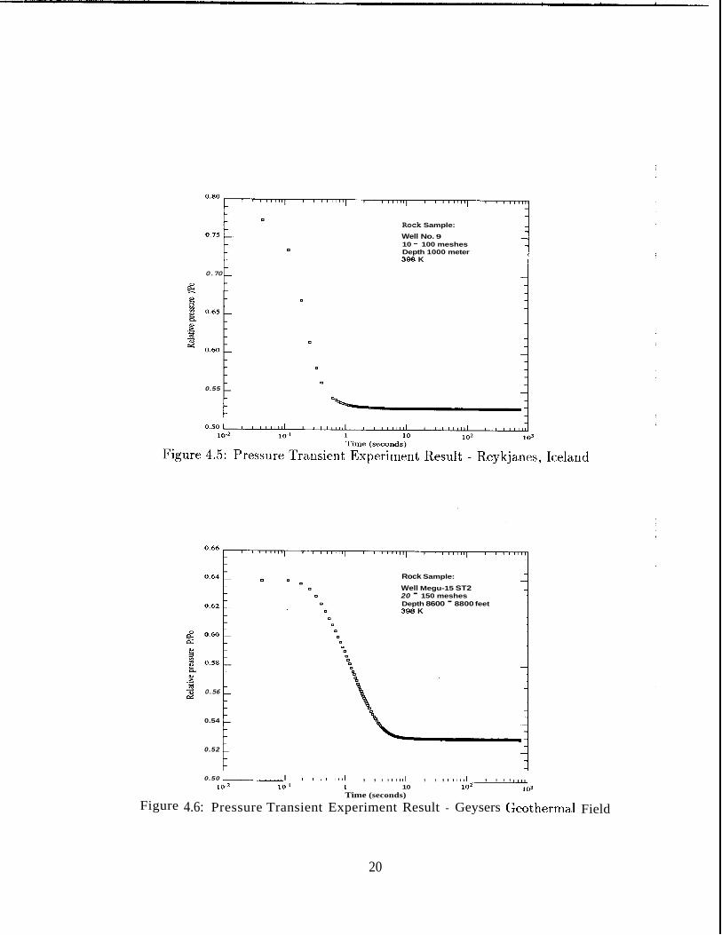
in Michael Harr’s report (1991). The eight experiment results are shown in Figure

4.1 through Figure 4.8. The corresponding isotherms.estimated from the experiments

are shown in Figure 4.9 through Figure 4.16.

4.2 Comparison of the Results

All results showed more or less similar pressure decline curves on a semilog plot. Some

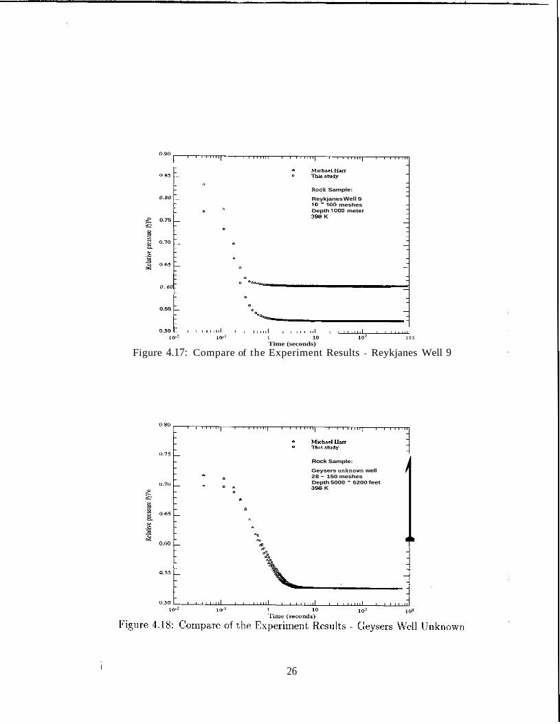
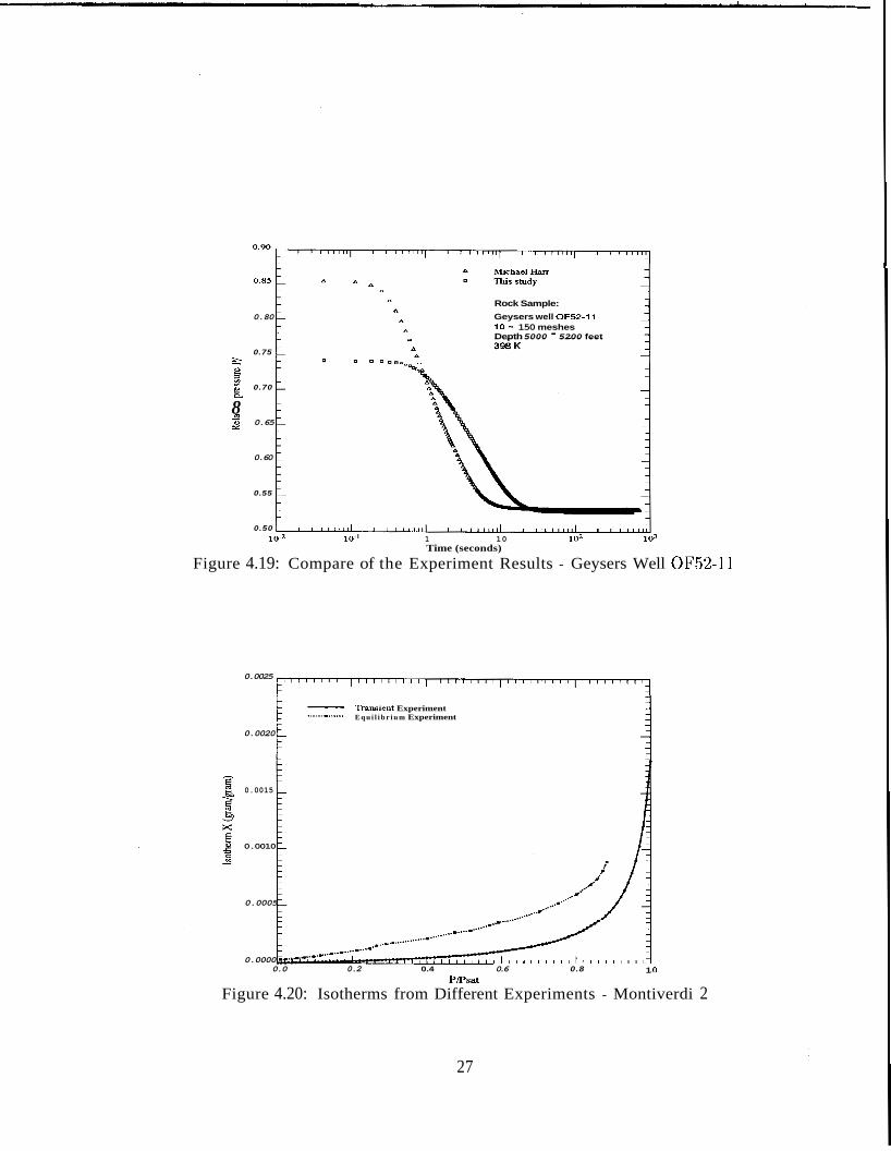
of the results are compared with Michael Harr’s results. They are shown i n Figures

4.17, 4.18, and 4.19. There are pressure differences between some of our results

and Michael Harr’s results. As shown in Figures 4.17 and 4.19, the starting relative

pressures are much lower than that of Michael Harr’s results. This was probably

caused by using different sample holders in case of Figure 4.19. Two sample holders

yere used by Michael Harr: one is 2.362 centimeters in diameter and 31.7 centimeters

in length and another is 1.727 c,cntimeters in diameter and 30.63 centimeters in length.

There is a short tube connecting the sample holder and pressure transducer with a

valve in between. Every time we measured the steam pressure, we evacuated the

tube first and then opened the valve. Thus part of steam flowed from sample into

this short empty tube. This lowered the steam pressure inside the sample holder.

When the large sample holder was used (Michael Harr’s case), this effect was not

significant. However for the small sample holder, the space inside the empty tube

was relatively large compared with the space inside the sample itself. When the

valve opened, a relatively large amount of steam flowed out of the sample to fill the

empty space and the pressure drop was more severe than in large sample holder case.

This resulted in the relative pressure difference because the saturated vapor pressures

were same. Figure 4.18 shows another pair of results. The two results were more

comparable because the same sample holder was used. As in the case in Figure 4.17,

the difference was caused by the measuring error. The data in Michael Harr’s report

(1991) showed the pressures of atmosphere recorded after the run were 1.2365 bars at

top of the sample holder and 0.6022 bars at the bottom of the sample holder. Which

is clearly an error.

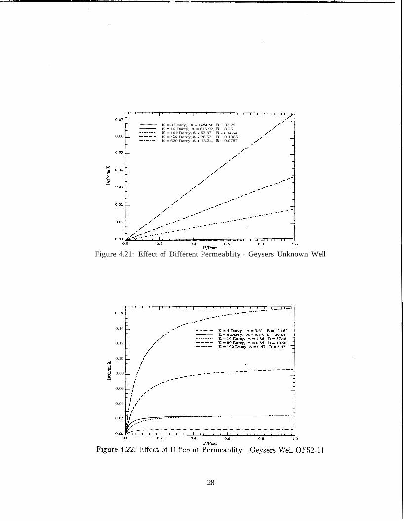
To check the validity of the isotherm estimation method, we need to compare

the results obtained by regression with the results obtained from experiment. There

are not many results available for the comparison. The only data available is the

isotherm measured from equilibrium experiment by Shang (1992). The same rock

sample was used in both transient and equilibrium experiments. The two results are

plotted together in Figure 4.20. The curves have very similar shape and the data are

reasonably close to each other. This is an encouraging sign.

There are many factors that affect the result of the transient flow experiment, such

as the temperature, the permeability, the porosity, particle size distribution, and the

sample rocks used, etc. The effects of permeability and porosity are discussed below.

All other effects are considered have less effect on the results of this experiment and

are not discussed.

16

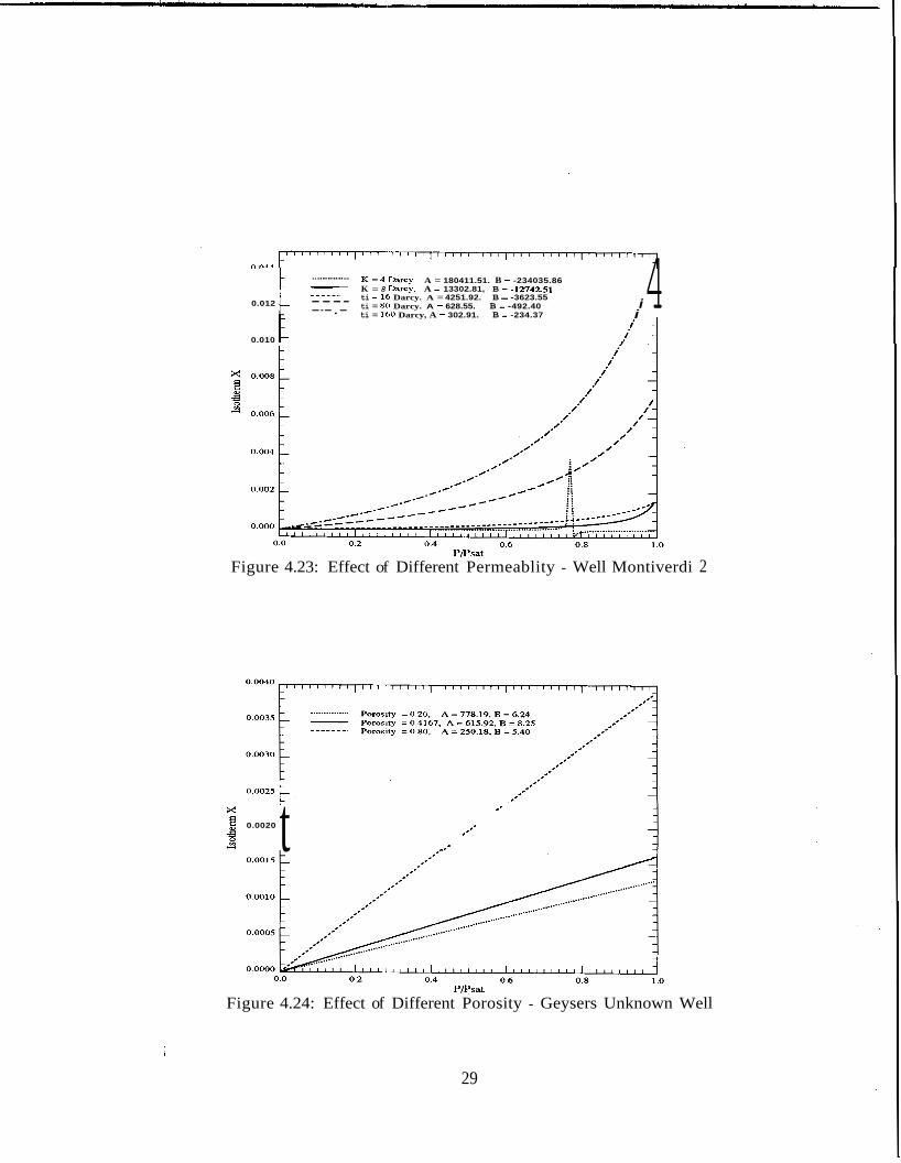
4.3 Effect of Permeability

The samples were prepared by pouring the presieved sample into the sample holder

with the holder being tapped to consolidate the sample as much as possible to gain

the largest sample weight. Permeability is measured after each transient run.

Three types of isotherm were obtained as shown earlier in Figure 4.9, Figure 4.11 and Figure 4.12: straight line, convex to the pressure axis, and concave to the pressure

axis. To examine the effect of permeability on the shape of the isotherms, different

permeabilities were used to do the nonlinear regression. The results are shown in

Figures 4.21, 4.22 and 4.23. From these figures we can see that although permeability

has a great effect on the numeric value of estimated isotherm, its variation does not

change the shape of the isotherm curve. This means that even when there is an error

in permeability or when there is no accurate permeability data available, we can still

use this method to do the estimation and obtain a consistent shape of the isotherm

curve.

4.4 Effect of Porosity

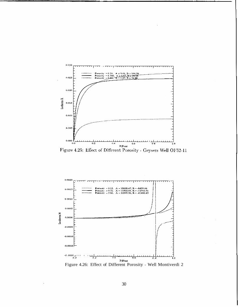
Porosities are calculated by knowing the volume of the sample holder and the weight

of the samples. In all calculations, a value of 2.70 gram per cubic centimeter is used.

To check the effect, the program were run by using different porosities rather than the

calculated ones. Again the results show that the porosity only affects the numerical

values of the isotherm being estimated but has no effect on the shape of the isotherm

curves. The results of the isotherm plot using different porosities are shown in Figures

4.24, 4.25 and 4.26.

17

0.70 1 Rock Sample:

28 - 150 meshes Unknown Well

Depth 5000 - 5200 feet 398 K

0.50 I I I I , , , , , I , , , , , , , , I , I , , , , , , I , , , , , , , 10-2 10-1 1 1 0 102 103

Figure 4.1: Pressure Transient Experiment Result - Geysers Shallow Reservoir Time (seconds)

0'75 I 1 ' 0.60

0.65

Well OF52-11 10 - 150 meshes Depth 5000 - 5200 feet

18

Rock Sample:

Well OF52-11 20 - 150 meshes

398 K Depth 5000 - 5200 feet

g 0.62

8 0.60

.s 'd 0.58

0.52 0.54 1 -1

0.60

8 a 0.56

.s 1

0.52

Rock sample:

Well Montiverdi 2

398 K 10 - 150 meshes I

0.50 I I I I I I , , , I I , , , , / , , I , , , , , , , , I , , , , , , 10-2 10-1 1 IO 102 io3

Figure 4.4: Pressure Time (seconds)

Transient Experiment Result - Montiverdi, Italy

19

0.70

CL &

- Rock Sample: - Well No. 9 - 10 - 100 meshes - Depth 1000 meter 398 K

-

- - - - - - - - -

0.55 1 -I

Figure

0.56

0.54

0.52 1

Rock Sample:

Well Megu-15 ST2 - 20 - 150 meshes

398 K Depth 8600 - 8800 feet

- -

-

-

-

-

'L: -

- - 7

0.50 I I I 1 I I , , , I , , , , , , , , I , , , ,,,,,I , , , , , , , 10-2 10-1 1 10 102

Time (seconds) io3

4.6: Pressure Transient Experiment Result - Geysers Geothermal Field

20

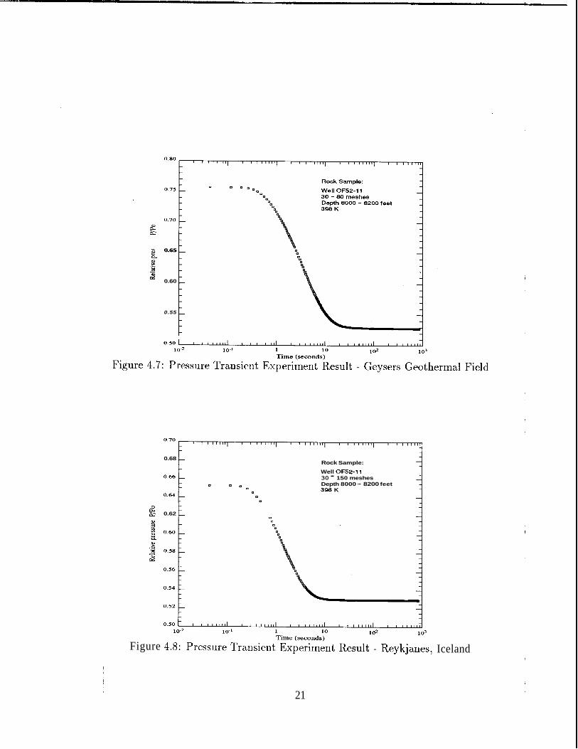
0.65

.z

' 0.60

0.55 1 c

0.68

0.62

Rock Sample:

Well OF52-11 30 - 150 meshes

398 K Depth 8000 - 8200 feet i

Figure Iceland

21

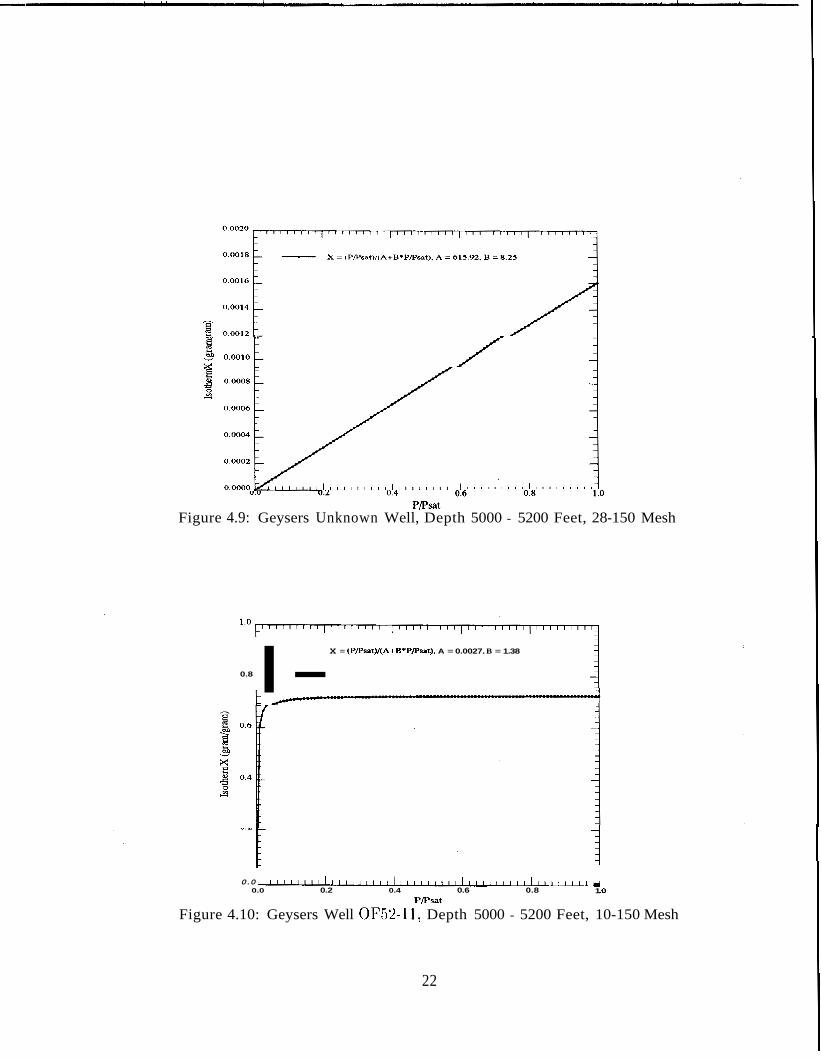
Figure 4.9: Geysers Unknown Well, Depth 5000 - 5200 Feet, 28-150 Mesh

I- X = (PlPsat)/(A+B'PlPsat). A = 0.0027. B = 1.38

0.8

0.0 1 1 1 1 ~ I I I I I , , I , , , , , , l , , , , , , , , , ~ , , , , l , , , , ~ , , , , l , , , , 0.0 0.2 0.4 0.6 0.8

P/P,t 1 .o

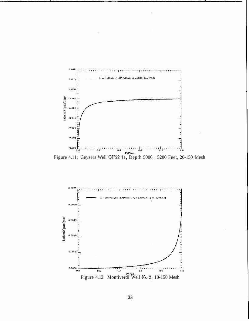
Figure 4.10: Geysers Well OF52-11, Depth 5000 - 5200 Feet, 10-150 Mesh

22

L - -

-

- - - - - - - - - -

- - 0.000.1 I I I I / ~ I I I I , , , , , , , , 1 / , , , , , , , , 1 , , , / , , , , , ~ , , , , , , , , , -

0.0 0.2 0.4 0.6 0.8 1.0 Ppsat

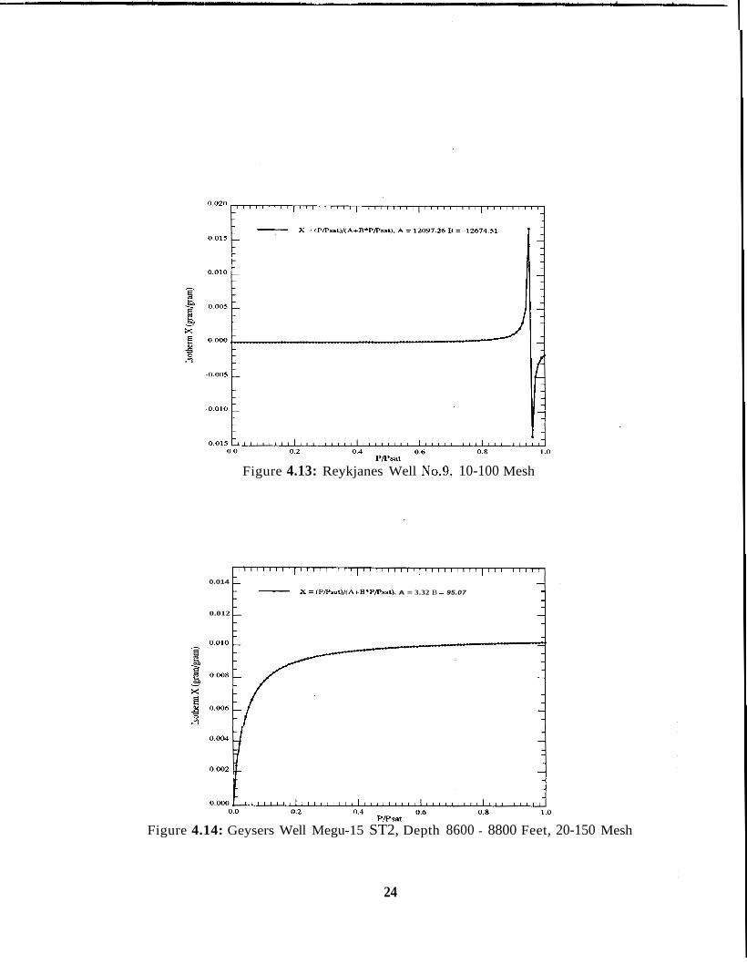
Figure 4.11: Geysers Well OF52-11, Depth 5000 - 5200 Feet, 20-150 Mesh

0.0020 1 x

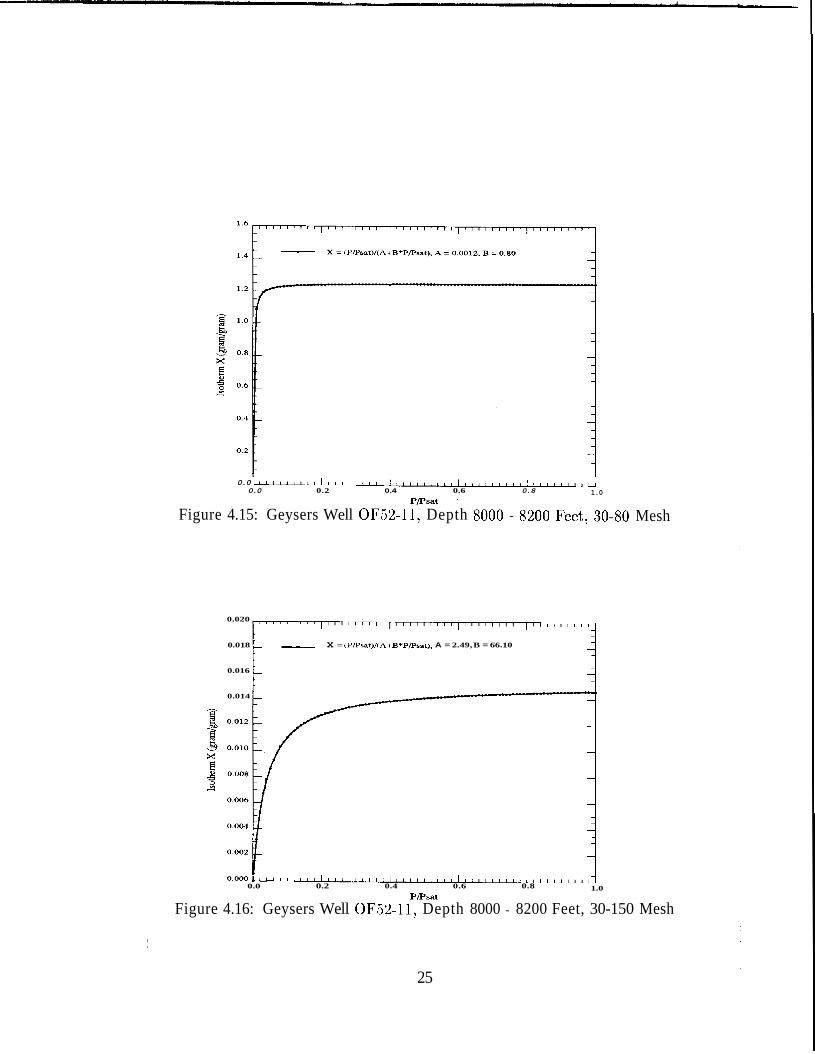
Figure 4.12: Montiverdi Well No.2, 10-150 Mesh

23

P/Psat

Figure 4.13: Reykjanes Well No.9, 10-100 Mesh

0.014

x = (PPsatlMA+B*PPsat). A = 3.32 B = 95.07

0.012 1

PPsat

Figure 4.14: Geysers Well Megu-15 ST2, Depth 8600 - 8800 Feet, 20-150 Mesh

24

0.0 I I I I I I I I I I I I I , 1 / , , , 1 1 , , , , , , , , 1 , , , 1 , , , , , ~ 1 , , , , , , , ,

0.0 0.2 0.4 0.6 0.8

PPsat '

1.0

Figure 4.15: Geysers Well OF52-11, Depth 8000 - 8200 Feet, 30-80 Mesh

0.020 1 " " " " ' I " " " " ' I " " " " ' ~ ' J I + I I I 1 8 -

- 0.018 - - X = (P/Psat)/(A+B*P/Psat). A = 2.49, B = 66.10 - - - - 0.016 - - -

- -

0.014 - -

-

-

-

- - - - - - - - - -

0.000.1r I I I / 1 1 1 1 1 , , , , , , , , 1 , , , , , , , , , ~ , , , , , , , , , ~ , , , , , , , , / - 0.0 0.2 0.4 0.6 0.8

PPsat 1.0

Figure 4.16: Geysers Well OF52-11, Depth 8000 - 8200 Feet, 30-150 Mesh

25

O u 5 l A

0.80 1 s 0.75

A

Rock Sample:

Reykjanes Well 9 10 - 100 meshes

398 K Depth 1000 meter

0.60 1 0.55 F

P

0 .5o t I I I 1 1 1 1 1 1 I , I , , / 1 , 1 , , , , , , , , I , , , , , / , ( I , , , , , , , 10-2 10-1 1 10 102 103

Figure 4.17: Compare of the Experiment Results - Reykjanes Well 9 Time (seconds)

B

A

P

n, -

A MichaclHarr Tbisstudy

Rock Sample:

Geysers unknown well 28 - 150 meshes

398 K Depth 5000 - 5200 feet 1

26

Rock Sample:

10 - 150 meshes Depth 5000 - 5200 feet

0.80 Geysers well OF52-11

0.75 &

g E 8

0.70

3 2 0.65

0.60

0.55

0.50 10-2 10-1 1 10 102 103

Time (seconds)

Figure 4.19: Compare of the Experiment Results - Geysers Well OF52-11

0.0025

- Transrent Experiment E q u i l i b r i u m Experiment

0.0020

0.0015

0.0010

0.0005

0.0000 0.0 0.2 0.4 0.6 0.8

PPsat 1 .o

Figure 4.20: Isotherms from Different Experiments - Montiverdi 2

27

............... K = 8 Darcy, A = 1484.58. B = 32.29 K = 1 6 Darcy, A = 615.92, B = 8.25 K = 1 6 0 Darcy, A = 53.37. B = 0.4664 K = 320 Darcy, A = 26.53. B = 0.1985 K = 620 Darcy. A = 13.24, B = 0.0787

0.06 x-

/-

P/Psat

Figure 4.21: Effect of Different Permeablity - Geysers Unknown Well

0.14

0.12

0.10

0.08

0.06

0.04

_----

28

. . . . . . . . . . . . . . . K = 4 Darcy, A = 180411.51. B = -234035.86 K = 8 Darcy. A = 13302.81, B = -12742.51 ti = 16 Darcy. A = 4251.92. B = -3623.55 ti = 80 Darcy. A = 628.55. B = -492.40 ti = 100 Darcy, A = 302.91. B = -234.37

- - - - - - - 0.012 ---- ---.- i

i 4 0.010 L

PPsat

Figure 4.23: Effect of Different Permeablity - Well Montiverdi 2

0.0020 t ..' .'

,.*'

P/Psat

Figure 4.24: Effect of Different Porosity - Geysers Unknown Well

29

x

-0.0005

-0.0010

-0.0015 I -0.0020 I I I I I I I , , r , , , , , , , , , l , , , , , , , , , r , , , , , , , , , l ; , , , , , , , , 1

Figure 4.26: Effect of Different Porosity - Well Montiverdi 2

0.0 0.2 0.4 0.6

P/Psat 0.8 1 .O

30

Chapter 5

Conclusions and Recommendations

5.1 Conclusions

0 By running the one-dinlensional steam flow simulator developed by Nghiem and

Ramey (1991) combined w i t h a nonlinear regression technique, the Langmuir

isotherm parameters can be estimated by using the pressure transient experi-

ment data.

0 The permeability value used i n the analysis does not affect the estimated shape

of the isotherm curve.

0 The porosity value used i n the analysis does not affect the estimated shape of

the isotherm curve.

0 The shape of the Langmuir isotherm curve depends heavily on the type of rock

used.

0 Particle size seems to have little effect on adsorption/desorption.

31

5.2 Recornmendat ions

0 The initial vapor pressure inside the sample holder is sensitive to the tempera-

ture changes in any part of the system. Great care must be taken to keep the

temperature as stable as possible.

0 The experimental procedures need to be modified in order to minimize the

effects of the open space between the ends of the sample holder and the pressure

transducers.

0 Whenever possible in the future, a larger sample holder should be used.

0 The one-dimensional simulator used only considered mass balance for simplicity.

An energy balance needs to be added to the model.

0 The experiments were all carried out at 125 degree C. Running experiments at

different temperatures in the future will enable us to examine the temperature

effect on the adsorption isotherm.

32

6. Nomenclature a =

A = b =

B = c =

co =

P = p* 1

P = Po =

P s a t =

P, =

R = s =

T = x = c =

equal distance between wells in x direction

constant

equal distance between wells in y direction

constant

constant

dimensionless wvllbore storage coefficient

gas or vapor pressure

saturated vapor pressure

gas or vapor pressure

saturated vapor pressure

saturation pressure

steam pressure

relative vapor pressure function

water saturation

absolute temperature

isotherm

experimental corlstant

33

Bibliography

[l] Fontana, F.: Memorie Mat. Fis. Soc. Ital Sci., 1, 679 (1777).

[2] Scheele, C.W.: Chemisch Adhandlung von der Luft und d e m Feuer, (1777).

[3] De Sauaaure, T.: Gilbert's Ann. der Physik, 22, 113, 1814.

[4] Calhoun, J.C., Lewis, M. Jr. and Newman, R.C.: Experiments on the Capil-

lary Properties of Porous Solids, Petroleum Transaction, AIME, 189-196, July,

(1949).

[5] Amyx, J.W., Bass, D.M. .Jr. and Whiting, R.L.: Petroleum Reservoir Engineer-

ing, McGraw-Hill Book Company, (1960).

[6] Whiting, R.L. and Ramey, H.J. Jr.: Application of Material and Energy Balances

to Geothermal Steam Production, Journal of Petroleum Technology, 893-900,

July, (1969).

[7] ItJPAC Manual of Symbols and Terminology, Appendix 2, Pt. 1, Colloid and

Surface Chemistry. Pure A p p l . Chem., 31, 578 (1972).

[8] Vargaftik, N.B.: Tables on the Thermophysical Properties of Liquids and Gases,

Second edition, Hemisphere Publishing Corporation, (1975).

[9] Brigham, W.E. and Morrow, W.B.: p/Z Behavior for Geothermal Steam Reser-

voirs, Society of Petroleum Engineers Journal, 407-412, December, (1977).

34

[lo] Moench, A.F. and Atkinson, P.G.: Transient-Pressure Analysis in Geothermal

Steam Reservoirs with an Immobile Vaporazing Liquid Phase, 253-264, Perga-

mon Press Ltd. (1978).

[ l l ] Udell, K.S.: The Thermodynamics of Evaporation and Condensation in Porous

Media, SPE 10779, 663-672, (1982).

[12] Gregg, S.J. and Sing, K.S.W.: Adsorption, Surface Area and Porosity, Second

Edition, Academic Press, (1982).

[13] Hsieh, C.H. and Ramey, H.J . Jr.: Vapor-Pressure Lowering in Geothermal Sys-

tems, Society of Petroleum Engineers Journal, February, 157-167 (1983).

[14] Economides, M.J.: Geothermal Reservoir Evaluation Considering Fluid Adsorp-

tion and Composition, Pl1.D. Thesis, Stanford University, (1983).

[15] Herkelrath, W.N., Moench, A.F. and O’Neal 11, C.F.: Laboratory Investigation

of Steam Flow in a Porous Medium, Water Resources Research, Vol. 19, No. 4, 931-937 (1983).

[16] Economides, M.J. and Miller, F.G.: The Effects of Adsorption Phenomena in

the Evaluation of Vapour-Dominated Geothermal Reservoirs, Geothermics, Vol.

14, No. 1, 3-27 (1985).

[17] Melrose, J.C.: Role of Capillary Condensation in Adsorption at High Relative

Pressure, Langmuir, Vol. 3, No. 5 , 661-667 (1987).

[18] Melrose, J.C.: Applicabi1it.y of the Kelvin Equation to Vapor/Liquid Systems in

Porous Media, Langmuir, Vol. 5 , No. 1, 290-293 (1989).

[19] Nghiem, C.P. and Ramey, H.J. Jr.: One-Dimensional Flow in Porous Media

Under Desorption, 16th Geothermal Workshop, Jan. (1991).

[20] Harr, M.S.: Laboratory Measurement of Sorption in Porous Media, Master’s

Report, Stanford University, August, (1991).

35

[21] Melrose, J.C.: Author’s Reply to discussion of Valid Pressure Data at Low

Wetting-Phase Saturation, SPE Reservoir Engineering, August, (1991).

[22] Nghiem, C.P. and Ramey. H..J. Jr.: One-Dimensional Steam Flow in Porous

Media, SGP No. TR-132, Stanford Geothermal Program, Stanford University,

(1991).

[23] Melrose, J.C., Dixon, J.R. and Mallinson, J.E.: Comparison of Different Tech-

niques for Obtaining Capillary Pressure Data in the Low Saturation Region, SPE

22690, (1991).

[24] Melrose, J.C.: Scaling Procedures for Capillary ,Pressure Data at Low Wetting-

Phase Saturations, SPE Formation Evaluation, 227-232, June (1991).

[25] Stanford Geothermal Program: Quarterly Report for April, May and June,

(1992).

36

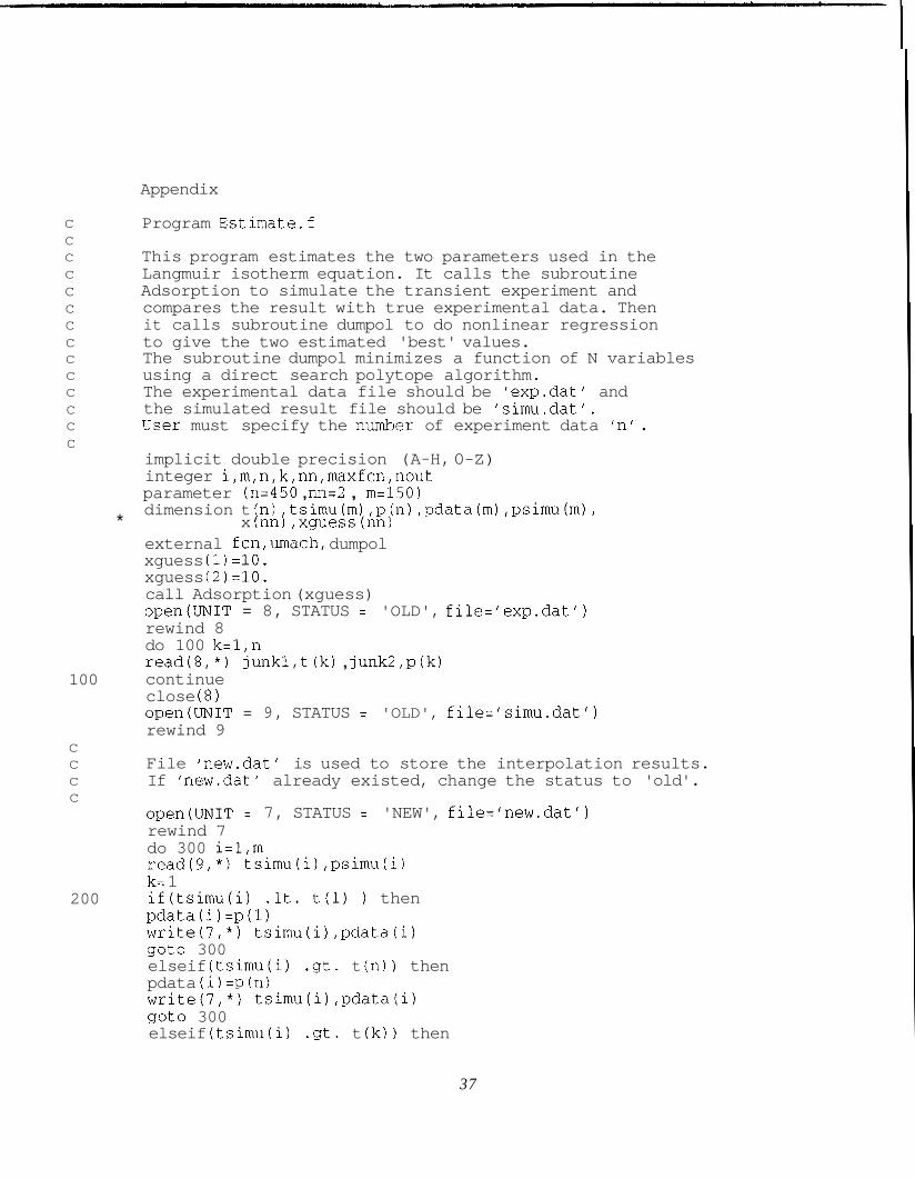
Appendix

C C C C C C C C C C C C C C

100

C C C C

200

Program Estimate.f

This program estimates the two parameters used in the Langmuir isotherm equation. It calls the subroutine Adsorption to simulate the transient experiment and compares the result with true experimental data. Then it calls subroutine dumpol to do nonlinear regression to give the two estimated 'best' values. The subroutine dumpol minimizes a function of N variables using a direct search polytope algorithm. The experimental data file should be 'exp.dat' and the simulated result file should be 'simu.dat'. TJser must specify the nunher of experiment data 'n' .

implicit double precision (A-H, 0-Z) integer i,m,n,k,nn,maxfcn,nout parameter (n=450 , nn=2 , m=150) dimension t (n) ,tsimu(m) ,p(n) ,pdata(m) ,psimu(m),

external fcn,umach, dumpol xguess ( 1) =lo. xguess (2 =lo. call Adsorption (xguess) open(UN1T = 8, STATUS = 'OLD', file='exp.dat') rewind 8 do 100 k=l,n read(8, * ) junk1,t (k) , junk2,p(k) continue close ( 8 open(UN1T = 9, STATUS = 'OLD', file='simu.dat') rewind 9

* x (nn) ,xguess (nn)

File 'new.dat' is used to store the interpolation results. If 'new.dat' already existed, change the status to 'old'.

open(UN1T = 7, STATUS = 'NEW', file='new.dat') rewind 7 do 300 i=l,m read(9, * ) tsimu(i) ,psimu(i)

if(tsimu(i) .It. t(1) then pdata(i)=p(l) write(7,*) tsimu(i) ,pdata(i) goto 300 elseif (tsimu(i) .gt. t (n) ) then pdata (i) =p (n) write(7,") tsimu(i) ,pdata(i) goto 300 elseif (tsimu(i) .gt. t (k) ) then

k= 1

37

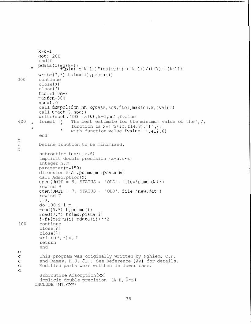
k=k+l got0 200 endi f pdata(i)=p(k-l)

write(7,*) tsimu(i) ,pdata(i) 300 continue

close (9) close (7 ftol=l.Oe-8 maxfcn=800 sss=l. 0 call dumpol(fcn,nn,xguess,sss,ftol,maxfcn,x,fvalue) call umach(2,nout) write (nout ,400 (x (k) , k=l , nn) , fvalue

* + (p (k) -p (k-1) ) * (tsimu (i) -t (k-1) ) / (t (k) -t (k-1) )

400 format ( ' The best estimate for the minimum value of the',/, * ' function is x= ( '2 (2x, f14.8) , ' 1 ' , / , * with function value fvalue= ',e12.6)

end C C C

100

Define function to be minimized.

subroutine fcn (n,x, f) implicit double precision (a-h,o-z) integer n,m parameter (m=150) dimension x(n) ,psimu(m) ,pdata (m) call Adsorption (x) open(UN1T = 9, STATUS = 'OLD', file='simu.dat') rewind 9 open(UN1T = 7, STATUS = 'OLD', file='new.dat') rewind 7 f=O. do 100 i=l,m read(9, * ) t,psimu(i) read(7, * ) tsimu,pdata(i) f=f+(psimu(i) -pdata(i) 1 **2 continue close (9 close (7 ) write(*,*) x,f return end

This program was originally written by Nghiem, C.P. and Ramey, H.J. Jr.. See Reference [ 223 for details. Modified parts were written in lower case.

subroutine Adsorption (xx) implicit double precision (A-H, 0-z)

INCLUDE 'M1.CM"

38

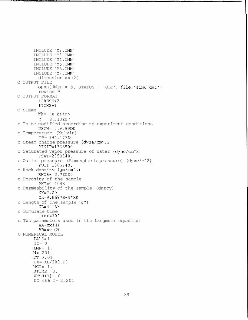
INCLUDE 'M2.C"' INCLUDE 'M3.C"' INCLUDE 'M4.C"' INCLUDE 'M5.C"' INCLUDE 'M6.C"' INCLUDE 'M7.C"' dimension xx (2)

open(UN1T = 9, STATUS = 'OLD', file='simu.dat') rewind 9

C OUTPUT FILE

C OUTPUT FORMAT IPRESS=2 ITIME=l

C STEAM WM= 18.015DO R= 8.3 13E07

c To be modified according to experiment conditions DSTW= 0.9589DO

c Temperature (Kelvin) TP= 394.177DO

c Steam charge pressure (dyne/cmA)2

c Saturated vapor pressure of water (dyne/cm"2)

c Outlet pressure (Atmospheric pressure) (dyne/cA2)

c Rock density (gm/cmA3 )

c Porosity of the sample

c Permeability of the sample (darcy)

PINIT=1338500.

PSAT=2050140.

POUT=1085240.

RHOR= 2 .7 0 OD0

PHI=0.4048

XK=7.00 XK=9.8697E-9*XK

c Length of the sample (cm)

c Simulate time

c Two parameters used in the Langmuir equation

XL=30.63

TIME=3 0 0.

AA=xx ( 1 ) BB=xx (2 )

C NUMERICAL MODEL IADS= 1 IC= 0 XMF= 1. N= 201 DT=O. 01 DX= XL/200.DO WGT= 1. STIME= 0. XMSH(1)= 0. DO 666 I= 2,201

39

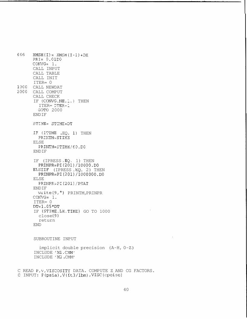
666 XMSH(I)= XMSH(1-1)+DX PRI= 0.01DO CONVG= 1. CALL INPUT CALL TABLE CALL INIT ITER= 0

1000 CALL NEWDAT 2000 CALL COMPUT

CALL CHECK IF (CONVG.NE. 1. ) THEN ITER= ITER+l GOT0 2000

END IF

STIME= STIME+DT

IF (ITIME . EQ. 1) THEN ELSE

END IF

PRINTM=STIME

PRINTM=STIME/GO.DO

IF (IPRESS .EQ. 1) THEN PRINPR=PI(201)/10000.DO

ELSEIF (IPRESS .EQ. 2) THEN PRINPR=PI(201)/1000000.D0

ELSE PRINPR=PI (201) /PSAT

Write (9, * ) PRINTM, PRINPR END IF

CONVG= 1. ITER= 0 DT=1,05*DT IF (STIME.LE.TIME) GO TO 1000 close (9) return

END

SUBROUTINE INPUT

implicit double precision (A-H, 0-Z) INCLUDE 'M1.CM" INCLUDE ' M2 . CMM

C READ P,v,VISCOSITY DATA. COMPUTE Z AND CG FACTORS. c INPUT: P(psia),v(ft3/lbrn) ,VISC(cpoise)

40

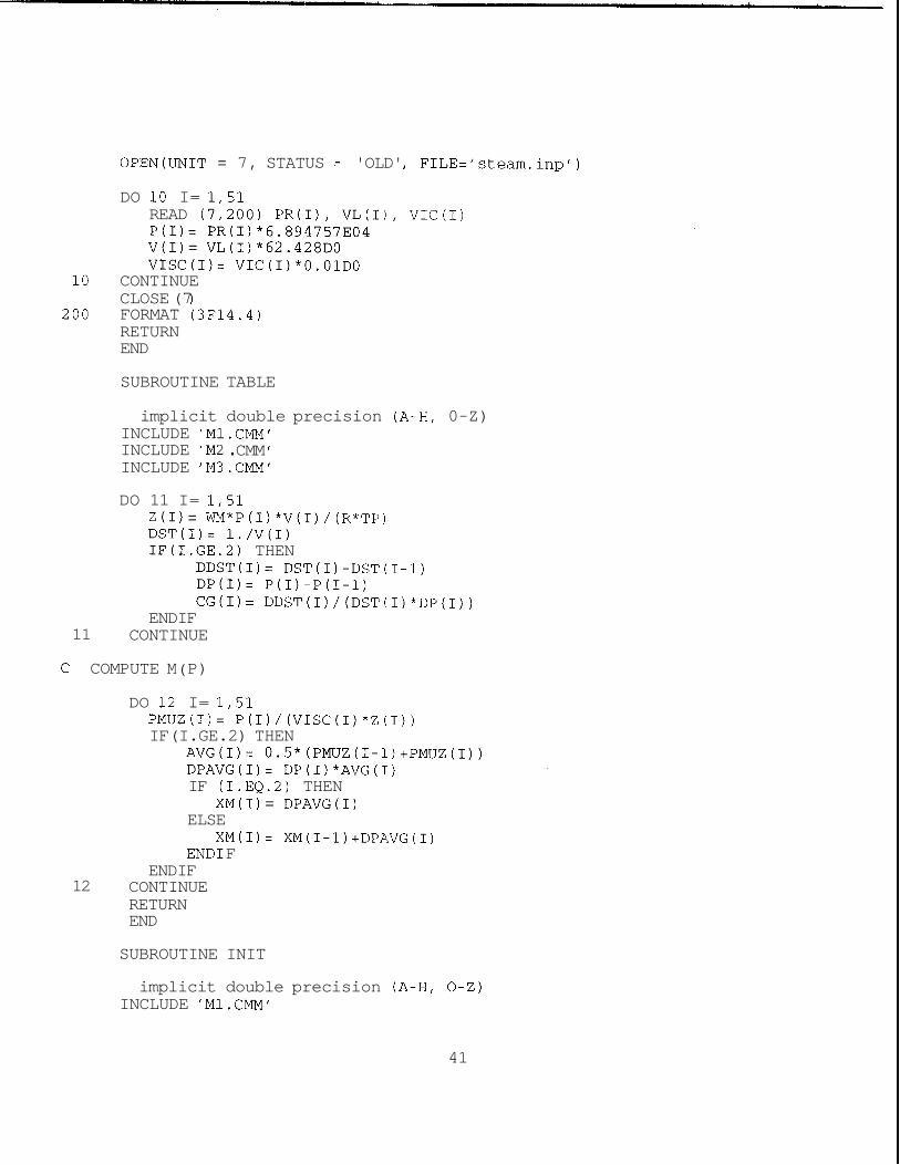
OPEN(UN1T = 7, STATUS = 'OLD' I FILE='steam.inp')

DO 10 I= 1,51 READ (7,200) PR(I), VL(II, VIC(1) P(I)= PR(I)*6.894757E04 V(1) = VL(1) *62.428DO VISC(I)= VIC(I)*O.OlDO

10 CONTINUE CLOSE (7 )

RETURN END

200 FORMAT (3F14.4)

SUBROUTINE TABLE

implicit double precision (A-H, 0-Z) INCLUDE 'M1.CM" INCLUDE ' M2 . CMM ' INCLUDE 'M3.CMM'

11

DO 11 I= 1,51 Z (1) = WM*P (I) *V(I) / (R*TP) DST(I)= l./V(I) IF(I.GE.2) THEN

DDST(I)= DST(1)-DST(1-1) DP(I)= P(1)-P(I-1) CG(I)= DDST(I)/(DST!I)*DP(I))

ENDIF CONTINUE

C COMPUTE M ( P)

12

DO 12 I= 1,51 PMUZ(I)= P(I)/(VISC(I)*Z(I)) IF(I.GE.2) THEN

AVG(I)= 0.5*(PMUZ(I-l)+PMUZ(I)) DPAVG(I)= DP(I)*AVG(I) IF (I.EQ.2) THEN

ELSE

END1 F

XM(1) = DPAVG(1)

XM(I)= XM(I-I)+DPAVG(I)

ENDIF CONTINUE RETURN END

SUBROUTINE INIT

implicit double precision (A-H, 0-Z) INCLUDE 'M1.CM"

41

INCLUDE ' M2 . CMM ' INCLUDE 'M3.CMM' INCLUDE 'M4.CMM' INCLUDE 'M5.CMM'

C INITIALIZE. FIND CORRESPONDING Z, VISCOSITY AND CG

DO 13 I= 1,201 IF (I .EQ. 1) THEN IF(IC.EQ.0) THEN

PI (I) = POUT ELSE

PI (I) = PINIT ENDI F

ELSE

ENDI F 13 CONTINUE

PO= PI (201) P1= PI(1) DO 91 I= 2'51

PI (I)= PINIT

PP(I-l)= P(1) XMM(I-1)= XM(1) CGG(I-l)= CG(1)

91 CONTINUE RETURN END

SUBROUTINE NEWDAT

implicit double precision (A-H, 0 - Z ) INCLUDE 'M1.CMM' INCLUDE ' M2 . CMM ' INCLUDE 'M3.C"' INCLUDE 'M4.CM" INCLUDE 'M5.CMM'

C KLINKERBERG EFFECT

SP= 0. DO 5 I= 1,201

5 SP= SP+PI (I PN= SP/201. XKK= XK*(1.+1.4E05/PN) DO 30 K= 1,201 IF(STIME.EQ.0.) THEN

CALL TABSEQ (PP'XMM, 50, PI (K) ,XMI (K) ELSE IF(IC.EQ.0) THEN

IF(K.GE.2 .AND.K.LE.201) XMI (K)= XMN(K)

42

ELSE

END1 F XMI (K) = XMN(K)

ENDIF CALL TABSEQ(P,VISC,51,PI(K),VISCI(K)) CALL TABSEQ(P,Z151,PI(K),ZI(K)) CALL TABSEQ(PP,CGG,SO,PI(K),CGI(K))

3 0 CONTINUE RETURN END

SUBROUTINE COMPUT

implicit double precision (A-H, 0 - Z )

INCLUDE 'M1.C"' INCLUDE M2 . CMM ' INCLUDE 'M3.C"' INCLUDE 'M4.C"' INCLUDE 'M5.CMM' INCLUDE 'M6.CM" INCLUDE 'M7.C"'

C COMPUTE MATRIX COEFFICIENT

17

* *

*

DO 17 I= 1,201 X(I)= PI(I)/(AA*PSAT+BB*PI(I)) DXDP( I) = AA*PSAT/ (AA*PSAT+BB*PI (I) ) **2 AI (11 = PHI*WM*VISCI (I) *CGI (I)

* *(l.-X(I)*RHOR*(l.-PHI)/(DSTW*PHI)) A2(I)= -DXDP(I)*(l.-PHI)*VISCI(I)*RHOR*m/DSTW IF (CONVG. EQ. 1. ) THEN A3(I)= DXDP(I)*ZI(I)*R*VISCI(I)*TP*RHOR*~1.-PHI)

* /PI (I) END IF

CONTINUE B= XKK*WM IF(IC.EQ.1) THEN

A(I)= Al(I)+A2(I)+A3(1)

DO 177 I= 1,201 IF(I.EQ.l) THEN D1(I)= l.+2.*B"WGT*DT/(A(I)*DX**2) Ul(I)= -2.*B*WGT*DT/(A(I)*DX**2) S1( I) = 2. *B*DT*R*TP*XMF/ (A (I) *DX*WM)

+(1.-2.*B*(I.-WGT)*DT/(A(I)*DX**2))*XMI(I) +2. *B* (1.-WGT) *DT*XMI (I+I) / (A(1) *DX**2)

ELSEIF(I.EQ.201) THEN D1(I)= l.+2.*B*WGT*DT/(A(I)*DX**2) TI (I) = -2. *B*WGT*DT/ (A ( I) *DX* "2 ) Sl(I)= (1.-2.*BX(1.-WGT)*DT/(A(I)*DX**2))*XMI(I)

+2.*B*(l.-WGT)*DT*XMI(1-1)/(A(I)*DX**2)

43

ELSE D1(I)= 1.+2.*B*WGT*DT/(A(I)*DX**2) TI (I) = -WGT*B*DT/ (A(1) *DX**2) U1 (I) = T1 (I) SI(I)= B * ( 1 . - W G T ) * D T * ( X M I ( I + l ) + X M I ( I - 1 ) ) / 0 ( I ) * D X * * 2 ) * +XMI(I)*(1.-2.*B*(I.-WGT)*DT/(A(I)*DX**2))

END IF 177 CONTINUE

CALL THOMAS(1,201,Tl,Dl,U1,Sl) DO 81 I= 1,201

81 XMN(1) = s1 (I) ELSE DO 188 I= 2,201 IF (I.EQ.2) THEN DI(I-I)= 1.+2.*B*WGT*DT/(A(I)*DX**2) U(I-1)= -B*WGT*DT/ (A(1) *DX**2) S(I-1)= B*DT*XMI(I-l) / (A(I)*DX**2) * +B*(l.-WGT)*DT*XMI(I+I)/(A(I)*DX**2)

* +(1.-2.*B*(1.-WGT)*DT/(A(I)*DX**2))*XMI(I) ELSEIF(I.EQ.201) THEN DI(I-I)= 1.+2.*B*WGT*DT/(A(I)*DX**2) T(1-I)= -2.*B*WGT*DT/(A(I)*DX**2) S(1-I)= (l.-2.*B*(l.-WGT)*DT/(A(I)*Dx**2))*XMI(I) * + 2 . * B * ( 1 . - W G T ) * D T * X M I ( I - 1 ) / ( A o ) * D X * * 2 )

ELSE DI(I-I)= 1.+2.*B*WGT*DT/(A(I)*DX**2) T(1-1)= -WGT*B*DT/ (A(1) *DX**2) U(I-1)= T(1-1) S(1-111 B * ( 1 . - W G T ) * D T * ( X M I ( I + 1 ) + X M I o ) / ( A ( I - l ) ) / ( A ( I ) * D X * * 2 )

* +XMI(I)*(1.-2.*B*(I.-WGT)*DT/(A(I)*DX**2)) END IF

CALL THOMAS(1,200,T,DI,U,S) DO 90 I=1,200

188 CONTINUE

XMN(I+l)= S(1) 90 CONTINUE

END1 F

C NEW PRESSURE IN CORE

IF(IC.EQ.0) THEN

ELSE NI= 2

NI= 1 END IF DO 40 I= NI,201

CALL TABSEQ(XMM,PP,5O,XMN(I),PI(I)) 40 CONTINUE

DO 41 I= NI,201 CALL TABSEQ(P,DST,51,PI(I) ,DSTO(I))

41 CONTINUE

44

RETURN END

SUBROUTINE CHECK

implicit double precision (A-H, 0 - Z ) INCLUDE 'M1.CM" INCLUDE 'M2 . CMM ' INCLUDE 'M3.C"' INCLUDE 'M4.CM" INCLUDE 'M5.CM" INCLUDE 'M6.CMM' INCLUDE ' M7 . CMM DO 1 I= 1,201 PCK(I)= PSAT*AA*X(I)/(~.-BB*X(I) SS(I)= (X(I)*RHOR*(1.-PHI))/(DSTW*PHI)

1 CONTINUE CONVG= 1. DO 2 I= 1,201 IF(ABS(PI(1)-PCK(1)) .GT.100000.) THEN

CONVG= CONVG+l. CALL TABSEQ(P,DST,~I,PCK(I),DSTAR(I)) A3(I)= A3(1)+PHI*(l.-SS(I))*(DSTAR(I)-DSTO(I))/DT IF(I.GE.2) XMI(I)= XMN'(1)

CONVG= COWG+O. ELSE

END I F 2 CONTINUE

RETURN END

C SEQUENTIAL SEARCH AND LINEAR INTERPOLATION

SUBROUTINE TABSEQ(X,Y,N,XX,YY)

implicit double precision (A-H, 0 - Z ) dimension X(*) ,Y(*)

I= 1

IF(1.GT.N) GO TO 98 IF(XX.GT.X(I)) GO TO 100 YY= Y(I-l)+(Y~I)-Y(I-l))*~xx-x(I-l))/~x~I~-x~I-l)) RETURN

98 YY= Y(N) RETURN END

100 I= 1+1

SUBROUTINE THOMAS (IL,IU,BB,DD,AA,CC) implicit double precision (A-H, 0 - Z )

45

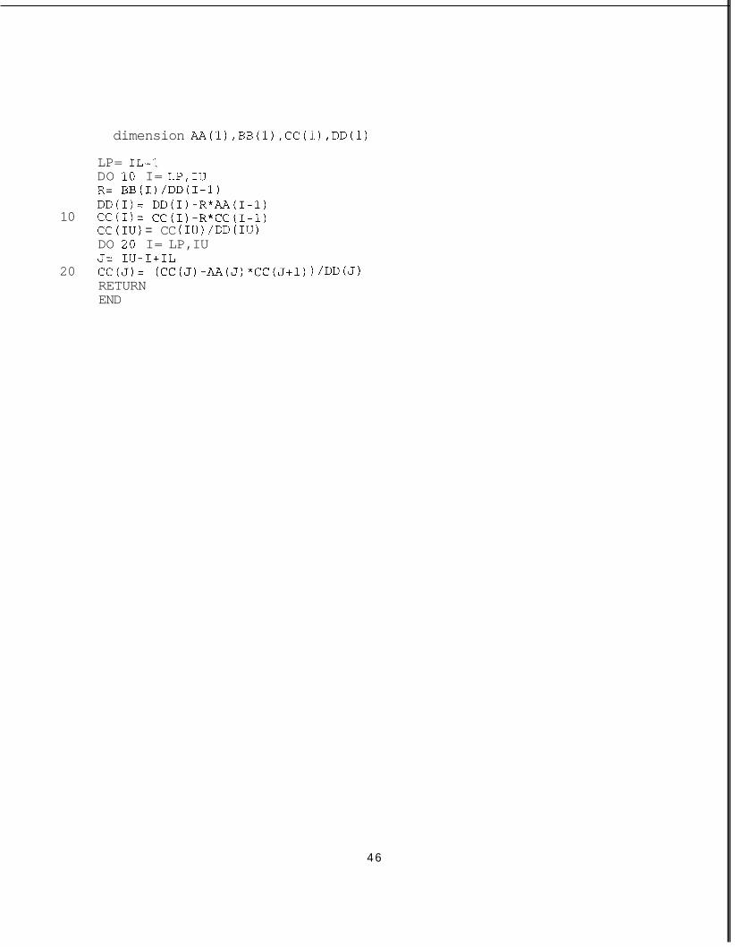
dimension AA(1) ,BB(l) ,CC(i) ,DD(l)

LP= IL+1 DO 10 I= LP,IU R= BB(I) l ~ ~ ( 1 - 1 ) DD(I)= DD(I)-R*AA(I-l)

10 CC(I)= CC(I)-R*CC(I-l) CC (IU) = CC (IU) /DD (IU) DO 20 I= LP, IU J= IU-I+IL

20 CC(J)= (CC(J)-AA(J)*CC(J+I) )/DD(J) RETURN END

4 6