Embed Size (px)
Citation preview
Estimation After a Group Sequential Trial
Elasma Milanzi1 Geert Molenberghs1,2 Ariel Alonso3
Michael G. Kenward4 Anastasios A. Tsiatis5 Marie Davidian5
Geert Verbeke2,1
1 I-BioStat, Universiteit Hasselt, B-3590 Diepenbeek, Belgium2 I-BioStat, Katholieke Universiteit Leuven, B-3000 Leuven, Belgium
3 Department of Methodology and Statistics, Maastricht University, the Netherlands4 Department of Medical Statistics, London School of Hygiene and Tropical Medicine,
London WC1E7HT, United Kingdom5 Department of Statistics, North Carolina State University, Raleigh, NC, U.S.A.
Abstract
Group sequential trials are one important instance of studies for which the sample size isnot fixed a priori but rather takes one of a finite set of pre-specified values, dependent on theobserved data. Much work has been devoted to the inferential consequences of this design feature.Molenberghs et al (2012) and Milanzi et al (2012) reviewed and extended the existing literature,focusing on a collection of seemingly disparate, but related, settings, namely completely randomsample sizes, group sequential studies with deterministic and random stopping rules, incompletedata, and random cluster sizes. They showed that the ordinary sample average is a viableoption for estimation following a group sequential trial, for a wide class of stopping rules andfor random outcomes with a distribution in the exponential family. Their results are somewhatsurprising in the sense that the sample average is not optimal, and further, there does not existan optimal, or even, unbiased linear estimator. However, the sample average is asymptoticallyunbiased, both conditionally upon the observed sample size as well as marginalized over it.By exploiting ignorability they showed that the sample average is the conventional maximumlikelihood estimator. They also showed that a conditional maximum likelihood estimator is finitesample unbiased, but is less efficient than the sample average and has the larger mean squarederror. Asymptotically, the sample average and the conditional maximum likelihood estimator areequivalent.
This previous work is restricted however to the situation in which the the random sample sizecan take only two values, N = n or N = 2n. In this paper, we consider the more practicallyuseful setting of sample sizes in a the finite set {n1, n2, . . . , nL}. It is shown that the sampleaverage is then a justifiable estimator , in the sense that it follows from joint likelihood estimation,and it is consistent and asymptotically unbiased. We also show why simulations can give thefalse impression of bias in the sample average when considered conditional upon the sample size.The consequence is that no corrections need to be made to estimators following sequential trials.When small-sample bias is of concern, the conditional likelihood estimator provides a relativelystraightforward modification to the sample average. Finally, it is shown that classical likelihood-based standard errors and confidence intervals can be applied, obviating the need for technical
1
corrections.
Some Keywords: Exponential Family; Frequentist Inference; Generalized Sample Average;Joint Modeling; Likelihood Inference; Missing at Random; Sample Average.
1 Introduction
Principally for ethical and economic reasons, group sequential clinical trials are in common use (Wald,
1945; Armitage, 1975; Whitehead, 1997; Jennison and Turnbull, 2000). Tools for constructing such
designs, and for testing hypotheses from the resulting data, are well established both in terms of
theory and implementation. By contrast, issues still surround the problem of estimation (Siegmund,
1978; Hughes and Pocock, 1988; Todd, Whitehead, and Facey, 1996; Whitehead, 1999) following
such trials. In particular, various authors have reported that standard estimators such as the sample
average are biased. In response to this, various proposals have been made to remove or at least
alleviate this bias and its consequences (Tsiatis, Rosner, and Mehta, 1984; Rosner and Tsiatis,
1988; Emerson and Fleming, 1990). An early suggestion was to use a conditional estimator for this
Blackwell (1947).
To successfully address the bias issue, it is helpful to understand its origins. Lehman (1950) showed
that it stems from the so-called incompleteness of the sufficient statistics involved, which in turn
implies that there can be no minimum variance unbiased linear estimator. Liu and Hall (1999) and
Liu et al (2006) explored this incompleteness in group sequential trials, for outcomes with both
normal and one-parameter exponential family distributions. For these distributions, Molenberghs
et al (2012) and Milanzi et al (2012) embedded the problem in the broader class with random
sample size, which includes, in addition to sequential trials, incomplete data, completely random
sample sizes, censored time-to-event data, and random cluster sizes. In so doing, they were able to
link incompleteness to the related concepts of ancillarity and ignorability in the missing-data sense.
By considering the conventional sequential trial with a deterministic stopping rule as a limiting
case of a stochastic stopping rule, these authors were able to derive properties of families of linear
estimators as well as likelihood-based estimators. The key results are as follows:(1) there exists a
maximum likelihood estimator that conditions on the realized sample size (CL), which is finite sample
unbiased, but has slightly larger variance and mean square error (MSE) than the SA ;(2) the sample
average (SA) exhibits finite sample bias, although it is asymptotically unbiased; (3) apart from the
exponential distribution setting, there is no optimal linear estimator, although the sample average
2
is asymptotically optimal; (4) the validity of the sample average as an estimator also follows from
standard ignorable likelihood theory.
Evidently, the CL is unbiased both conditionally and marginally with respect to the sample size. By
contrast, the CL is marginally unbiased, but there exist classes of stopping rules where, conditionally
on the sample size, there is asymptotic bias for some values of the sample sizes. Surprisingly, this is
not of concern. Milanzi et al (2012) showed this for the case of two possible sample sizes, N = n
and N = 2n. With such a stopping rule, it is possible that, for example when N = n, the bias
grows unboundedly with n; when this happens though, the probability that N = n shrinks to 0 at
the same rate. If strict finite sample unbiasedness is regarded as essential, the conditional MLE can
be used, which, like MLE, also admits the standard likelihood-based precision measures, although
it is computationally intensive. This is a very important result and should be contrasted with the
various precision estimators that have been developed in the past.
On the other hand, developments in Molenberghs et al (2012) and Milanzi et al (2012) show that
despite finite sample bias, a correction may not be strictly necessary for SA. Further, its likelihood
basis, implies it can be used in conjunction with standard likelihood-based measures of precision,
such as standard errors and associated confidence intervals to provide valid inferences.
A major limitation of Molenberghs et al (2012) and Milanzi et al (2012) is the restriction to two
looks of equal size. It is the main aim of this paper to extend this work to the practically more useful
setting of multiple looks of potentially different sample sizes.
In Section 2, we introduce notation, describe the setting, the models, and the associated generic
problem. In Section 3, we study the problems of incompleteness when using a stochastic stopping
rule. The class of generalized sample averages in introduced in Section 6, and conditional and joint
maximum likelihood estimators are derived in Section ??. Their asymptotic properties are studied in
Section 7. A simulation study is described in the Supplementary Materials, Section A.
2 Problem and Model Formulation
Consider a sequential trial with L pre-specified looks, with sample sizes n1 < n2 < . . . , < nL. Assume
that there are nj i.i.d. observations Y1, . . . , Ynj , from the jth look that follow an exponential family
distribution with density
fθ(y) = h(y) exp {θy − a(θ)} , (1)
3
for θ the natural parameter, a(θ) the mean generating function, and h(y) the normalizing constant.
Subsequent developments are based on a generic data-dependent stochastic stopping rule, which we
write
π(N = nj |knj ) = F(knj
∣∣ψ) = F(knj
), (2)
where Knj =∑nj
i=1 Yi also has an exponential family density:
fnj (k) = hnj (k) exp{θknj − nja(θ)
}. (3)
Our inferential target is the parameter θ, or a function of this.
2.1 Stochastic Rule As A Group Sequential Stopping Rule
. While the stopping rule seems different from the ones frequently used, it will later on be clear as
to how it can be specified to conform to the commonly used stopping rules in the sequential trials.
For instance, when the conditional probability of stopping of an exponential family form is chosen,
e.g.,
F (kn) = F (k) =
∫ z=A(k)
z=−∞f1(z)dz, (4)
then an appealing form for the marginal stopping probability can be derived. Here f1(z) can be
seen as an exponential family member, underlying the stopping process. When the outcomes Y
and hence K do not range over the entire real line, the lower integration limit in (4) should be
adjusted accordingly, and the function A(k) should be chosen so as to obey the range restrictions. It
is convenient to assume that f1(z) has no free parameters; should there be the need for such, then
they can be absorbed into A(k). Hence, we can write
f1(z) = h1(z) exp {−a(0)} . (5)
Using (3) and (5), the marginal stopping probability becomes:
P (N = n) =
∫ k=+∞
k=−∞
∫ z=A(k)
z=−∞fn,θ(k)f1(z)dz dk
= exp {−na(θ)− a(0)}∫ k=+∞
k=−∞hn(k)
[∫ z=A(k)
z=−∞h1(z)dz
]eθkdk
= exp {−na(θ)− a(0)}L {H1(A(k)) · hn(k)} , (6)
where
H1(t) =
∫ z=t
z=−∞h1(z)dz.
4
Milanzi et al (2012) studied in detail the behavior of stopping rules where
A(k) = αj + βknj/nmj
, where αj , β and m are constants specific to a design.
Choosing β →∞ and β → −∞ results into deterministic stopping or continuing thus corresponding
to the stopping rules commonly used in sequential trials. The trial is stopped when (6) is greater than
a randomly generated number from uniform(0,1). Note that the higher the evidence against(for) the
null hypothesis, the higher the probability to stop. In the specific example of normally distributed
responses (1) can be chosen as standard normal. The value of α is paramount to deciding the behavior
of stopping boundaries. Consider O’Brien and Fleming stopping boundaries where it is difficult to
stop in early stages; one can then specify αj such that the probability of stopping increases with
the stages. In addition to the computational advantages and the associated practicality, we use the
stochastic rule to maintain the focus of this paper, which is estimation.
3 Incomplete Sufficient Statistics
Several concepts play a crucial role in determining the properties of estimators following sequential
trial: incompleteness, a missing at random (MAR) mechanism, ignorability, and ancillarity (Molen-
berghs et al , 2012). We consider the role of incompleteness first: a statistic s(Y ) of a random
variable Y , with Y belonging to a family Pθ, is complete if, for every measurable function g(·),
E[g{s(Y )}] = 0 for all θ, implies that Pθ[g{s(Y )} = 0] = 1 for all θ (Casella and Berger, 2001,
pp. 285–286). Incompleteness is central to the various developments (Liu and Hall, 1999; Liu et al ,
2006; Molenberghs et al , 2012) because of the the Lehman-Scheffe theorem which states that “if a
statistic is unbiased, complete, and sufficient for some parameter θ, then it is the best mean-unbiased
estimator for θ,” (Casella and Berger, 2001). In the present setting, the relevant sufficient statistic
is not complete, and so the theorem can not be applied here.
In line with extending the work of Molenberghs et al (2012) and Milanzi et al (2012), to a general
number of looks, we explore incompleteness and its consequencies in studies with more than two
looks using the stochastic rule.
In a sequential setting, a convenient sufficient statistic is (K,N). Following the developments in the
5
above papers, the joint distribution for (K,N) is:
p(K,N) = f0(K,N) F (KN ), (7)
f0(kn1 , n1) = fn1(kn1), (8)
f0(knj , nj) =
∫f0(knj−1 , nj−1)fnj−nj−1(knj − knj−1)
[1− F (knj−1)
]dknj−1 . (9)
If (K,N) were complete, then there would exist a function g(K,N) such that E [g(K,N)] = 0 if
and only if g(K,N) = 0, implying that
0 =
∫g(kn1 , n1)fn1(kn1)F (kn1)dkn1 +
L−2∑j=2
∫g(knj , nj)H(knj )F (knj )dknj
+
∫g(knL , nL)H(knL)F (knL)dknL , (10)
with
H(knj ) =
∫ . . .︸︷︷︸j−1
∫f0(knj−1 , nj−1)fnj−nj−1(knj − knj−1)
[1− F (knj−1)
]dkn1 . . . dknj−1
].
Tedious but straightforward algebra results into:
g(knL , nL)H(knL) = −L−1∑j=1
∫g(zj , nj)H(zj)F (zj)dzj ,
g(knL , nL) =
∑L−1j=1
∫g(zj , nj)H(zj)F (zj)dzj
H(knL).
Assigning, for example, arbitrary constants to g(n1, kn1) . . . g(nL−1, knL−1), a value can be found
for g(nL, knL) 6= 0, contradicting the requirement for (K,N) to be complete, hence establishing
incompleteness. From applying the Lehmann-Scheffe theorem, that no best mean-unbiased estimator
is guaranteed to exist. The practical consequence of this is that even estimators as simple as a sample
average need careful consideration and comparison with alternatives. Nevertheless, the situation is
different for non-linear mean estimators as illustrated for the conditional likelihood estimator.
4 Unbiased Estimation: Conditional Likelihood
The eminent draw back of linear based mean estimators in the context of sequential trials is their
finite sample bias. In connecting missing data and sequential trials theory, Molenberghs et al (2012)
provided a factorization for the joint distribution of observed data and sample size that leads to an
6
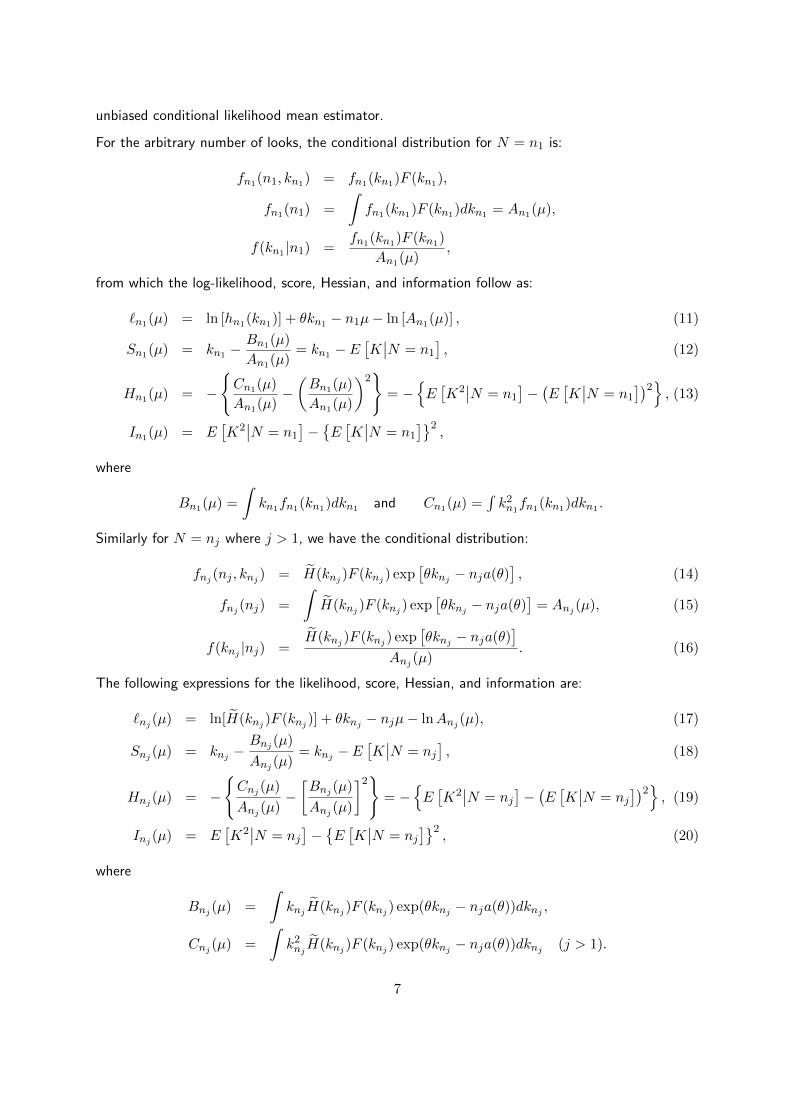
unbiased conditional likelihood mean estimator.
For the arbitrary number of looks, the conditional distribution for N = n1 is:
fn1(n1, kn1) = fn1(kn1)F (kn1),
fn1(n1) =
∫fn1(kn1)F (kn1)dkn1 = An1(µ),
f(kn1 |n1) =fn1(kn1)F (kn1)
An1(µ),
from which the log-likelihood, score, Hessian, and information follow as:
`n1(µ) = ln [hn1(kn1)] + θkn1 − n1µ− ln [An1(µ)] , (11)
Sn1(µ) = kn1 −Bn1(µ)
An1(µ)= kn1 − E
[K∣∣N = n1
], (12)
Hn1(µ) = −
{Cn1(µ)
An1(µ)−(Bn1(µ)
An1(µ)
)2}
= −{E[K2∣∣N = n1
]−(E[K∣∣N = n1
])2}, (13)
In1(µ) = E[K2∣∣N = n1
]−{E[K∣∣N = n1
]}2,
where
Bn1(µ) =
∫kn1fn1(kn1)dkn1 and Cn1(µ) =
∫k2n1
fn1(kn1)dkn1 .
Similarly for N = nj where j > 1, we have the conditional distribution:
fnj (nj , knj ) = H(knj )F (knj ) exp[θknj − nja(θ)
], (14)
fnj (nj) =
∫H(knj )F (knj ) exp
[θknj − nja(θ)
]= Anj (µ), (15)
f(knj |nj) =H(knj )F (knj ) exp
[θknj − nja(θ)
]Anj (µ)
. (16)
The following expressions for the likelihood, score, Hessian, and information are:
`nj (µ) = ln[H(knj )F (knj )] + θknj − njµ− lnAnj (µ), (17)
Snj (µ) = knj −Bnj (µ)
Anj (µ)= knj − E
[K∣∣N = nj
], (18)
Hnj (µ) = −
{Cnj (µ)
Anj (µ)−[Bnj (µ)
Anj (µ)
]2}= −
{E[K2∣∣N = nj
]−(E[K∣∣N = nj
])2}, (19)
Inj (µ) = E[K2∣∣N = nj
]−{E[K∣∣N = nj
]}2, (20)
where
Bnj (µ) =
∫knjH(knj )F (knj ) exp(θknj − nja(θ))dknj ,
Cnj (µ) =
∫k2nj
H(knj )F (knj ) exp(θknj − nja(θ))dknj (j > 1).
7
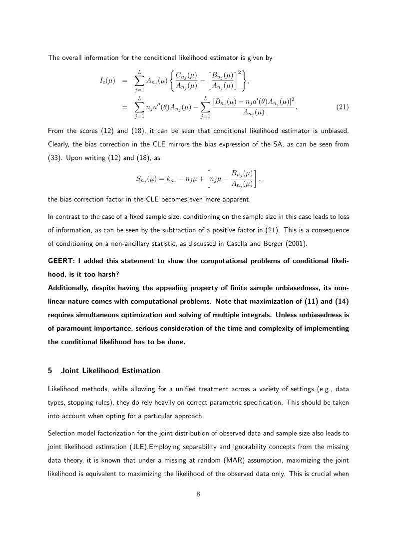
The overall information for the conditional likelihood estimator is given by
Ic(µ) =L∑j=1
Anj (µ)
{Cnj (µ)
Anj (µ)−[Bnj (µ)
Anj (µ)
]2},
=
L∑j=1
nja′′(θ)Anj (µ)−
L∑j=1
[Bnj (µ)− nja′(θ)Anj (µ)]2
Anj (µ). (21)
From the scores (12) and (18), it can be seen that conditional likelihood estimator is unbiased.
Clearly, the bias correction in the CLE mirrors the bias expression of the SA, as can be seen from
(33). Upon writing (12) and (18), as
Snj (µ) = knj − njµ+
[njµ−
Bnj (µ)
Anj (µ)
],
the bias-correction factor in the CLE becomes even more apparent.
In contrast to the case of a fixed sample size, conditioning on the sample size in this case leads to loss
of information, as can be seen by the subtraction of a positive factor in (21). This is a consequence
of conditioning on a non-ancillary statistic, as discussed in Casella and Berger (2001).
GEERT: I added this statement to show the computational problems of conditional likeli-
hood, is it too harsh?
Additionally, despite having the appealing property of finite sample unbiasedness, its non-
linear nature comes with computational problems. Note that maximization of (11) and (14)
requires simultaneous optimization and solving of multiple integrals. Unless unbiasedness is
of paramount importance, serious consideration of the time and complexity of implementing
the conditional likelihood has to be done.
5 Joint Likelihood Estimation
Likelihood methods, while allowing for a unified treatment across a variety of settings (e.g., data
types, stopping rules), they do rely heavily on correct parametric specification. This should be taken
into account when opting for a particular approach.
Selection model factorization for the joint distribution of observed data and sample size also leads to
joint likelihood estimation (JLE).Employing separability and ignorability concepts from the missing
data theory, it is known that under a missing at random (MAR) assumption, maximizing the joint
likelihood is equivalent to maximizing the likelihood of the observed data only. This is crucial when
8
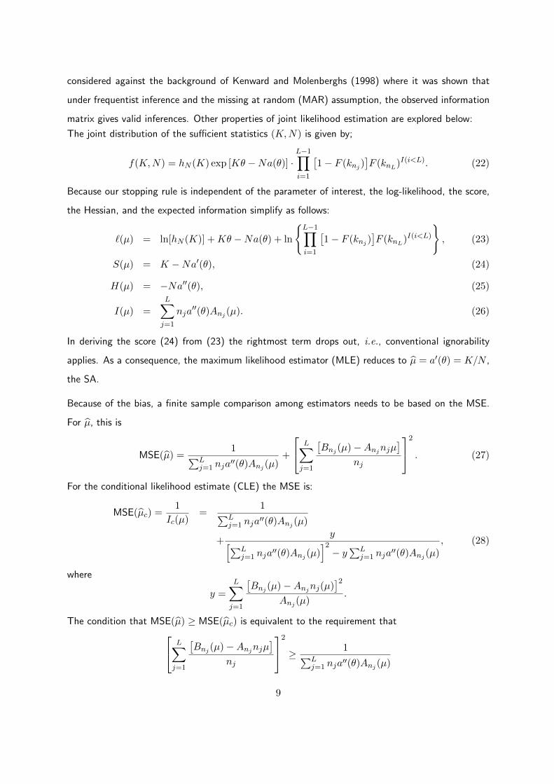
considered against the background of Kenward and Molenberghs (1998) where it was shown that
under frequentist inference and the missing at random (MAR) assumption, the observed information
matrix gives valid inferences. Other properties of joint likelihood estimation are explored below:
The joint distribution of the sufficient statistics (K,N) is given by;
f(K,N) = hN (K) exp [Kθ −Na(θ)] ·L−1∏i=1
[1− F (knj )
]F (knL)I(i<L). (22)
Because our stopping rule is independent of the parameter of interest, the log-likelihood, the score,
the Hessian, and the expected information simplify as follows:
`(µ) = ln[hN (K)] +Kθ −Na(θ) + ln
{L−1∏i=1
[1− F (knj )
]F (knL)I(i<L)
}, (23)
S(µ) = K −Na′(θ), (24)
H(µ) = −Na′′(θ), (25)
I(µ) =
L∑j=1
nja′′(θ)Anj (µ). (26)
In deriving the score (24) from (23) the rightmost term drops out, i.e., conventional ignorability
applies. As a consequence, the maximum likelihood estimator (MLE) reduces to µ = a′(θ) = K/N ,
the SA.
Because of the bias, a finite sample comparison among estimators needs to be based on the MSE.
For µ, this is
MSE(µ) =1∑L
j=1 nja′′(θ)Anj (µ)
+
L∑j=1
[Bnj (µ)−Anjnjµ
]nj
2
. (27)
For the conditional likelihood estimate (CLE) the MSE is:
MSE(µc) =1
Ic(µ)=
1∑Lj=1 nja
′′(θ)Anj (µ)
+y[∑L
j=1 nja′′(θ)Anj (µ)
]2− y
∑Lj=1 nja
′′(θ)Anj (µ), (28)
where
y =
L∑j=1
[Bnj (µ)−Anjnj(µ)
]2Anj (µ)
.
The condition that MSE(µ) ≥ MSE(µc) is equivalent to the requirement that L∑j=1
[Bnj (µ)−Anjnjµ
]nj
2
≥ 1∑Lj=1 nja
′′(θ)Anj (µ)
9
holds. For the special case of equal sample sizes this can never be true, hence the SA has the smaller
MSE. More generally, neither is uniformly superior in terms of MSE.
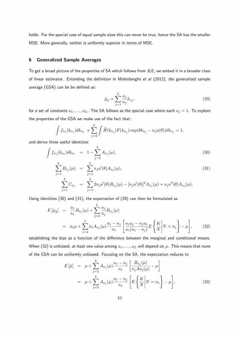
6 Generalized Sample Averages
To get a broad picture of the properties of SA which follows from JLE, we embed it in a broader class
of linear estimator. Extending the definition in Molenberghs et al (2012), the generalized sample
average (GSA) can be be defined as:
µg =L∑j=1
ajnjknj , (29)
for a set of constants a1, . . . , aL. The SA follows as the special case where each aj = 1. To explore
the properties of the GSA we make use of the fact that:∫fn1(kn1)dkn1 +
L∑j=2
∫H(knj )F (knj ) exp(θknj − nja(θ))dknj = 1,
and derive three useful identities:∫fn1(kn1)dkn1 = 1−
L∑j=2
Anj (µ), (30)
L∑j=1
Bnj (µ) =L∑j=1
nja′(θ)Anj (µ), (31)
L∑j=1
Cnj =
L∑j=1
2nja′(θ)Bnj (µ)− [nja
′(θ)]2Anj (µ) + nja′′(θ)Anj (µ),
Using identities (30) and (31), the expectation of (29) can then be formulated as
E [µg] =a1n1Bn1(µ) +
L∑j=2
ajnjBnj (µ)
= a1µ+L∑j=2
a1Anj (µ)n1 − njn1
[n1aj − nja1a1(n1 − nj)
E
{K
N
∣∣∣∣∣N = nj
}− µ
], (32)
establishing the bias as a function of the difference between the marginal and conditional means.
When (32) is unbiased, at least one value among a1, . . . , aL will depend on µ. This means that none
of the GSA can be uniformly unbiased. Focusing on the SA, the expectation reduces to
E [µ] = µ+
L∑j=2
Anj (µ)n1 − njn1
[Bnj (µ)
njAnj(µ)− µ
]
= µ+L∑j=2
Anj (µ)n1 − njn1
[E
{K
N
∣∣∣∣∣N = nj
}− µ
], (33)
10
from which we get the bias as
L∑j=2
Anj (µ)n1 − njn1
[Bnj (µ)
njAnj(µ)− µ
]=
L∑j=2
n1 − njn1nj
[Bnj (µ)−Anjnjµ
]=
L∑j=1
[Bnj (µ)−Anjnjµ
]nj
. (34)
Thus, the SA is unbiased when the conditional and marginal means are equal.
7 Asymptotic Properties
We now turn to the large-sample properties of the estimators discussed in the previous sections. When
N →∞, approximately K ∼ N(Nµ,Nσ2), so normal-theory arguments can be used. Considering a
first-order Taylor series expansion of F (knj ) around njµ results in F (knj ) ≈ F (njµ)+F ′(njµ)(knj−
njµ). Without loss of generality, consider a class of stopping rules for which F ′(nj)n→∞→ 0. In this
setting, the expressions derived above can be approximated by
An1(µ) ≈ F (n1µ),
Bn1(µ) ≈ F (n1µ)n1µ,
Anj (µ) ≈j−1∏i=1
[1− F (niµ)]F (njµ), (j > 1)
Bnj(µ) ≈j−1∏i=1
[1− F (niµ)]F (njµ)njµ, (j > 1).
These approximations will be useful in what follows.
7.1 Asymptotic Bias
Conditional Likelihood Estimation
We turn now to the asymptotic conditional behavior of the bias of the sample average given the
sample size. Two cases are considered:
Case I. F (nµ)n→∞−→ a ∈]0, 1[ and F ′(nµ)
n→∞−→ 0. For this case E[µ|N = nj ]n→∞−→ µ, for j =
1, . . . , L.
Case II. Here, both the function F (·) and its first derivative F (·) converge to zero. When this
happens, it does so for all but one of the sample sizes that can possibly be realized. The one
11
exception is the sample size that will be realized, asymptotically, with probability one. Without
loss of generality, we illustrate this case for stopping at the first look, assuming that the sample
size realized at the first look corresponds to a set of values for µ taht do not contain the true
one. Thus, F (nµ)n→∞−→ 0 and F ′(nµ)
n→∞→ 0. This case can correspond for particular forms
of F (knj ). Given that K is asymptotically normally distributed, letting F (K) = Φ(k) is a
mathematically convenient choice from which it follows that F (njµ) = Φ(njµ). Consider first
N = n1. Then,
limn1→∞
E[µ|N = n1] = µ− limn1→∞
φ(n1µ)σ2
Φ(n1µ),
of which the right hand term approaches 0/0. We therefore apply l’Hopital’s rule and obtain:
limn1→∞
E[µ|N = n1] = µ− limn1→∞
−n1µφ(n1µ)
φ(n1µ)→∞,
with the sign opposite to that of µ. Hence, conditional on the fact that stopping occurs after
the first look, the estimate may grow in an unbounded way. However, recalling that F (nµ),
the probability of stopping when N = n1, also approaches zero, these extreme estimates are
also extremely rare. In the same case, for N = nj (j > 1), limn→∞E[µ|N = nj ] → µ. So
for these sample sizes no asymptotic bias occurs.
Milanzi et al (2012) showed that a large class of stopping rules corresponds to either Case I or
Case II. For example, for stopping rule Φ(α + βk/n), they found that Case I applies. Switching to
Φ(α + βk), F ′(nµ) = βφ(α + βnµ) which again tends to zero. However, Φ(α + βnµ) may tend
to either zero or one. For a general rule F (k) = Φ(α + βknm), with m any real number, F ′(nµ)
converges to zero whatever m is. Further, F (nµ) converges to Φ(α + βµ) for m = −1, Φ(α) for
m < −1, and Φ(±∞) (i.e., 0 or 1) for m > −1.
Joint Likelihood Estimation
Recall that the bias for the SA was given by (34), which asymptotically tends to the limit
limn→∞
L∑j=1
∏j−1i=1 [1− F (niµ)]F (njµ)njµ−
∏j−1i=1 [1− F (niµ)]F (njµ)njµ
nj−→ 0.
Although the sample average is finite-sample biased in general for data-dependent stopping rules, it
is asymptotically unbiased and hence can be considered an appropriate candidate for practical use
following a sequential trial. Emerson (1988) established the same result for two possible looks and
further noted that this property is not relevant in group sequential trials, because large sample sizes are
12
unethical, hence making the study of small sample properties crucial. On the other hand, results from
a comprehensive analysis, comparing randomized controlled trials (RCTs) stopped for early benefit
(truncated) and RCTs not stopped for early benefit (non-truncated), indicated that treatment effect
was over-estimated in most of truncated RCTs regardless of the pre-specified stopping rule used
(Bassler et al , 2010). They further advocate stopping rules that demand large number of events. In
their exploration of properties of estimators, Milanzi et al (2012) showed that in the general class of
linear mean estimators, only the sample average has asymptotic unbiasedness property thus giving
it an advantage in cases where asymptotic unbiasedness would play a role. The sample average is
asymptotically unbiased in all cases, and even conditionally asymptotically unbiased, even in the case
of an arbitrary number of looks. Further, under the usual likelihood regularity conditions, the SA is
then consistent and asymptotically normally distributed, and the likelihood-based precision estimator
and its corresponding confidence intervals are valid. Care has to be exercised when working under
the MAR assumption, as it is the case here, because the observed information matrix rather than the
expected information matrix should be used to obtain precision estimators to ensure their validity.
Kenward and Molenberghs (1998) noted that, provided that use is made of the likelihood ratio,
Wald or score statistics based on the observed information, then reference to a null asymptotic χ2
distribution will be appropriate.
This conventional asymptotic behavior contrasts with the idiosyncratic small-sample properties of
the SA derived in the Section 6.
7.2 Asymptotic Mean Square Error
Given that the bias for the sample average tends to zero as the sample size increases and that∑Lj=1Bnj (µ)−Anj (µ)njµ
n→∞−→ 0, it follows that
limn→∞
MSE(µ) = limn→∞
MSE(µc)→1∑L
j=1 nja′′(θ)Anj (µ)
.
8 Simulation Study
8.1 Design
The simulation study has been designed to corroborate the theoretical findings on the behavior of
the likelihood estimators, in comparison to commonly used biased adjusted estimators. Assume a
clinical trial comparing a new therapy to a control, designed to follow O‘Brien and Fleming’s group
13
sequential plan with four interim analyses.
The objective of the trial is to show that the mean response from the new therapy is higher than that
of the control group. Let Yit ∼ N(µt, 1) and Yic ∼ N(µc, 1) be the responses from subject i in the
therapy and control groups, respectively. The null hypothesis is formulated as H0 : θ = µt − µc = 0
vs. H1 : θ = θ1 > 0. Further, allow a type I error of 2.5% and 90% power to detect the clinically
meaningful difference.
Given that we are interested in asymptotic behavior, different values of the clinically meaningful
difference, θ1 = 0.5, 0.25, and 0.15 are considered to achieve different sample sizes, with smaller θ1
corresponding to larger sample size.
With the settings described above, datasets are generated as follows; at each stage, Yit ∼ N(2, 1),
i = 1 . . . nj , j = 1 . . . 4 and Yic ∼ N(µc, 1), where µc = 1.5, 1.75, and 1.85 for the first, second, and
third setting, respectively. These also serve as the true mean values under which the bias is being
considered.
Estimation proceeds by obtaining the maximum likelihood estimator (sample average: µt − µc) at
each stage and apply the stopping rule:
F (knj ) = Φ
(αj + β
kjnj
), (j = 1 . . . 4),
where β = 100 to represent the rules applied to the group sequential trials case (Milanzi et al ,
2012). To follow the behavior of O’Brien and Fleming boundaries (where early stopping is difficult),
a value of α is chosen to make sure that the probability of stopping increases with the increase in
number of looks, i.e., αj = 2(h−j+1)h α1, where α1 = −50, −25, and−15 for θ1 = 0.5, 0.25, and 0.15,
respectively and h is the number of planned looks. Obviously, the choice of αj depends on the design
and goals of the trial. In this setting, α1 was chosen such that P (N = n3|θ = θ1) ≥ 0.5 and to make
early stopping difficult. The decision to stop is made when F (knj ) > U , where U ∼ Uniform(0, 1);
otherwise, we continue. For example if F (knj ) = 0.70, then the probability of continuing is 30% and
for large values of β, F (knj ) ∈ {0, 1}.
The objective of the simulation is to show that the performance of the CLE as the mean estimator
after a group sequential trial and compare MLE to other bias adjusted estimators.We further show
that MLE confidence intervals obtained by using the observed information matrix, lead to valid
conclusions.
14
Other estimators obtained include: the mean unbiased estimator (MUE), the bias adjusted estimator
(BAM; Todd, Whitehead, and Facey 1996), and Rao’s bias-adjusted estimator (RBADJ; Emerson
and Fleming 1990).
Additional simulations with two possible looks and a smaller value of β for both joint and conditional
likelihood are presented in the Appendix.
8.2 Results
Table 1 gives the mean estimates for different estimators of θ. On average MLE exhibits large
relative bias compared to the bias adjusted estimates, for example, for θ1 = 0.15 which corresponds to
maximum sample size of 1949, relative bias for MLE is 6% compared to 0.7% for CLE. The conditional
likelihood estimate performs as expected with consistent small bias in all the three scenarios. On the
other hand, MLE shows the asymptotic unbiasedness behavior, seen by the reduction (though small)
in relative bias as sample size increases. This is not the same for BAM and RBADJ.
While point estimates are useful in giving the picture of the magnitude of the difference, confidence
intervals (CI) are highly important in decision making. A comparison of adjusted confidence intervals
provided with the RCTdesign package in R (Emerson et al , 2012), to the likelihood based confidence
intervals, obtained by using observed variance as precision estimates, indicates that their coverage
probabilities are comparable. The coverage probabilities were (94.6%, 94.6%, 97.6%) for the adjusted
CI and (93.8%, 92.8%, 96.8%) for MLE based CI, for the three settings in the order of increasing
sample size. Using the same design parameters, we also investigated the type I error rate for MLE and
adjusted estimators, by setting θ1 = 0 and obtaining the percentage times the confidence interval
does not contain zero. Type I error rates for likelihood based CI were (5.6%,6.4%,2.8%), which
are similar to those based on adjusted CIs, (5.4%,4.8%,2.8%) for the three settings in the order
of increasing sample size. Certainly using either of the CIs will lead to similar conclusions, which
makes the simpler and well known sample average a good estimator candidate for analysis after group
sequential trials..
We also explore the bias of each of the estimators at the sample level in contrast to the averaged
bias as presented in Table 1. Recall that we had 500 samples for each setting, Table 2 gives the
proportion of samples whose estimates’ relative bias fell into a specified category. The CLE had a
reverse trend of the other estimators where a only few estimated had large bias. Indeed it is hard
15
to pick a preferred estimator among the others estimators based on these results since each of the
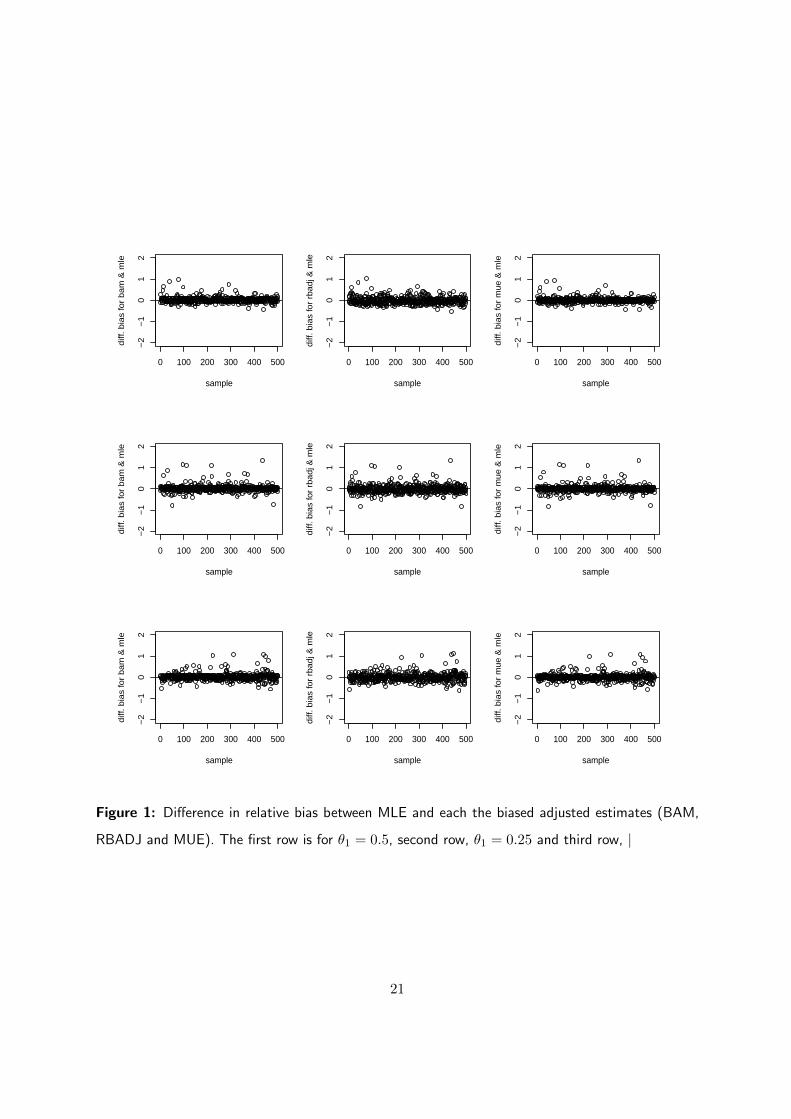
estimator has about 75% of the estimates having relative bias of > 10%. It is also clear from Figure
1, which plot the difference in relative bias, between each of the bias adjusted estimates and MLE,
that none of the estimates discussed above is uniformly unbiased in comparison to MLE, i.e is some
instances MLE may do better.
Table 1: Mean estimates (Est.) and relative bias (R.Bias) for the three different settings of O’Brien
and Fleming’s design. Parameters common to all the three settings include, power=90%, type I
error=0.025, H0 : θ = 0 vs. H1 : θ = θ1 > 0, where only the detectable difference (θ1) was changed
to initiate change in maximum sample size (Size). MLE is the maximum likelihood estimate, BAM
is the bias-adjusted maximum likelihood estimate, RBADJ is the Rao bias adjusted estimate, MUE
is the median unbiased estimate and CLE is the conditional likelihood estimate.
MLE BAM RBADJ MUE CLE
Size Est. R.Bias Est. R.Bias Est. R.Bias Est. R.Bias Est. R.Bias
176 0.5448 (0.0895) 0.5142 (0.0285) 0.5019 (0.0037) 0.5251 (0.0502) 0.5026 (0.0052)
702 0.2665 (0.0661) 0.2508 (0.0031) 0.2473 (0.0108) 0.2557 (0.0228) 0.2476 (0.0094)
1949 0.1595 (0.0635) 0.1489 (0.0070) 0.1469 (0.0209) 0.1520 (0.0130) 0.1511 (0.0071)
9 Concluding Remarks
As a result of the bias associated with joint maximum likelihood estimators following sequential
trials, much work has been applied to providing alternative estimators. The origin of the problem lies
with the incompleteness of the sufficient statistic for the mean parameter Lehman (1950), implying,
among others, that there is no best unbiased linear mean estimator.
Using stochastic stopping rules, which encompass the deterministic stopping rules used in sequential
trials as special cases, we have studied the properties of joint maximum likelihood estimators afresh, in
an attempt to enhance our understanding of the behavior of estimators (for both bias and precision)
based on data from such studies. This has been data for the one parameter exponential family
distributions to encompass response outcomes form several distributions like, binary , normal, Poisson,
16
Table 2: Results from three different settings of O’Brien and Fleming’s design. Parameters common
to all three settings include: power=90%, type I error=0.025, H0 : θ = 0 vs. H1 : θ = θ1 > 0, where
only the detectable difference (θ1) was changed to initiate change in maximum sample size (Size).
Out of 500 datasets generated for each setting, we compare the percentage of estimates (Prop. as
a percentage) whose relative bias falls in the specified range (R.Bias as a percentage). MLE is the
maximum likelihood estimate, BAM is the biased adjusted maximum likelihood estimate, RBADJ
is Rao’s bias adjusted estimate, MUE is the median unbiased estimate, and CLE is the conditional
likelihood estimate..
Prop.(%)
θ1(Size) R.Bias(%) BAM RBADJ MUE MLE CLE
0.5(176) ≤ 0.99 2.6 2.0 2.2 2.2 76.3
1− 4.99 8.4 11.4 11.0 10.6 13.2
5− 10 10.6 11.6 12.6 15.0 7.9
> 10 78.4 75.0 74.2 72.2 2.6
0.25(702) ≤ 0.99 2.0 3.2 1.4 2.6 81.3
1− 4.99 7.2 9.0 8.8 9.0 12.5
5− 10 9.4 9.8 10.8 9.8 2.1
> 10 81.4 78.0 79.0 78.6 4.2
0.15(1949) ≤ 0.99 2.6 1.8 1.4 2.2 55.6
1− 4.99 7.4 13.2 8.0 13.2 33.3
5− 10 9.2 9.0 11.8 11.0 8.9
> 10 80.8 76.0 77.6 74.4 2.2
exponential and survival times.
First, the incompleteness of the sufficient statistic when using a stochastic stopping rule has been
established. Using a generalized sample average, it is noted that in almost no case is there an
unbiased estimator. Even when such an estimator does exist, with a completely random sample size,
it cannot be uniformly best.
Second, there exist an unbiased estimator resulting from the likelihood of the observed data con-
ditional on the sample size. While appealing, the conditional estimator is computationally more
17
involved, because there is no closed-form solution. Although for a sequential trial with a determin-
istic stopping rule, the ordinary sample average is finite sample biased, it can be been shown both
directly and through likelihood arguments, that it is asymptotically unbiased and so remains a good
candidate for practical use. Further, it is computationally trivial, has a correspondingly simple esti-
mator of precision,derived from observed information matrix and hence a well behaved asymptotic
likelihood-based confidence interval. In addition, the mean square error of the sample average is
smaller than that of the estimator based on the conditional likelihood. Asymptotically, the mean
square errors of both estimators converge.
Third, there is the subtle issue that the sample average may be asymptotically biased for certain
stopping rules, when its expectation is considered conditionally on certain values of the sample size.
However, this is not a real practical problem because this occurs only for sample sizes that have
asymptotic probability zero of being realized. We placed emphasis on joint and conditional likelihood
estimators. While in the former the stopping rule is less present than sometimes thought, it is not
in the latter. Also, when alternative frequentist estimators are considered, the stopping rule is likely
to play a role in synchrony with the rule’s influence on hypothesis testing due to the duality between
hypothesis testing and confidence intervals.
While in some circumstances other sources of inaccuracy may overwhelm the issue studied here, we
believe it is useful to bring forward implications of our findings for likelihood-based estimation.
Our findings, especially for the simulations in the appendix, indicate that bias decreases relatively
rapidly with sample size, but there are subtle differences depending on stopping rule considered. In
this sense, fixed rules are different from Z-statistic based rules (Emerson 1988, p. 5; Jennison and
Turnbull, 2000).
In conclusion, the sample average is a very sensible choice for point, precision, and interval estimation
following a sequential trial.
Acknowledgments
Elasma Milanzi, Geert Molenberghs, Michael G. Kenward, and Geert Verbeke gratefully acknowledge
support from IAP research Network P7/06 of the Belgian Government (Belgian Science Policy). The
work of Anastasios Tsiatis and Marie Davidian was supported in part by NIH grants P01 CA142538,
R37 AI031789, R01 CA051962, and R01 CA085848.
18
References
Armitage, P. (1975) Sequential Medical Trials. Oxford: Blackwell.
Bassler, D., Briel, M., Montori, V. M., Lane, M., Glasziou, P., Zhou, Q., Heels-Ansedell, D., Walter,
S.D., Guyatt, G.H. and the STOPIT-2 Study Group. (2010). Stopping randomized trials early
for benefit and estimation of treatment effects. Systematic review and meta-regression analysis.
Journal of the American Medical Association,303, 1180–1187.
Blackwell, D. (1947). Conditional expectation and unbiased sequential estimation. Annals of Math-
ematical Statistics, 18 ,105-110.
Casella, G. and Berger, R.L. (2001). Statistical Inference. Pacific Grove: Duxbury Press.
Emerson, S.S. (1988). Parameter estimation following group sequential hypothesis testing. PhD
dissertation. University of Washington.
Emerson, S.S. and Fleming, T.R. (1990). Parameter estimation following group sequential hypothesis
testing. Biometrika, 77, 875–892.
Emerson,S.S., Gillen, D.L., Kittelson, J.K., Emerson, S.C., and Levin, G.P (2012). RCTdesign: Group
Sequential Trial Design. R package version 1.0.
Hughes, M.D. and Pocock, S.J. (1988). Stopping rules and estimation problems in clinical trials.
Statistics in Medicine, 7, 1231–1242.
Jennison, C. and Turnbull, B.W (2000). Group Sequential Methods With Applications to Clinical
Trials. London: Chapman & Hall/CRC.
Kenward, M.G. and Molenberghs, G. (1998) Likelihood based frequentist inference when data are
missing at random. Statistical Science, 13, 236–247.
Lehmann, E.L. and Stein, C. (1950). Completeness in the sequential case. Annals of Mathematical
Statistics,21, 376–385.
Liu, A. and Hall, W.J. (1999). Unbiased estimation following a group sequential test. Biometrika,
86, 71–78.
19
Liu, A., Hall, W.J., Yu, K.F., and Wu, C. (2006). Estimation following a group sequential test for
distributions in the one-parameter exponential family. Statistica Sinica, 16, 165–81.
Milanzi, E., Molenberghs, G., Alonso, A., Kenward, M.G., Aerts, M., Verbeke, G., Tsiatis, A.A., and
Davidian, M. (2012). Properties of estimators in exponential family settings with observation-based
stopping rules. Submitted for publication.
Molenberghs, G., Kenward, M.G., Aerts, M., Verbeke, G., Tsiatis, A.A., Davidian, M., Rizopoulos, D.
(2012). On random sample size, ignorability, ancillarity, completeness, separability, and degeneracy:
sequential trials, random sample sizes, and missing data. Statistical Methods in Medical Research,
00, 000–000.
Rosner, G.L. and Tsiatis, A.A. (1988). Exact confidence intervals following a group sequential trial:
A comparison of methods. Biometrika, 75, 723–729.
Siegmund, D. (1978). Estimation following sequential tests. Biometrika, 64, 191–199.
Tsiatis, A.A., Rosner, G.L., and Mehta, C.R. (1984). Exact confidence intervals following a group
sequential test. Biometrics, 40, 797–803.
Todd, S., Whitehead, J., and Facey, K.M. (1996). Point and interval estimation following a sequential
clinical trial. Biometrika, 83, 453–461.
Wald, A. (1945). Sequential tests of statistical hypotheses. The Annals of Mathematical Statistics,
16, 117-186.
Whitehead, J. (1997). The Design and Analysis of Sequential Clinical Trials (2nd ed.). New York:
John Wiley & Sons.
Whitehead, J. (1999). A unified theory for sequential clinical trials. Statistics in Medicine, 18, 2271–
2286.
20
0 100 200 300 400 500
−2
−1
01
2
sample
diff
. b
ias
for
ba
m &
mle
0 100 200 300 400 500
−2
−1
01
2
sample
diff
. b
ias
for
rba
dj &
mle
0 100 200 300 400 500
−2
−1
01
2
sample
diff
. b
ias
for
mu
e &
mle
0 100 200 300 400 500
−2
−1
01
2
sample
diff
. b
ias
for
ba
m &
mle
0 100 200 300 400 500
−2
−1
01
2
sample
diff
. b
ias
for
rba
dj &
mle
0 100 200 300 400 500
−2
−1
01
2
sample
diff
. b
ias
for
mu
e &
mle
0 100 200 300 400 500
−2
−1
01
2
sample
diff
. b
ias
for
ba
m &
mle
0 100 200 300 400 500
−2
−1
01
2
sample
diff
. b
ias
for
rba
dj &
mle
0 100 200 300 400 500
−2
−1
01
2
sample
diff
. b
ias
for
mu
e &
mle
Figure 1: Difference in relative bias between MLE and each the biased adjusted estimates (BAM,
RBADJ and MUE). The first row is for θ1 = 0.5, second row, θ1 = 0.25 and third row, |
21
Estimation After a Group Sequential Trial
Elasma Milanzi1 Geert Molenberghs1,2 Ariel Alonso3 Michael G. Kenward4
Anastasios A. Tsiatis5 Marie Davidian5 Geert Verbeke2,1
1 I-BioStat, Universiteit Hasselt, B-3590 Diepenbeek, Belgium
2 I-BioStat, Katholieke Universiteit Leuven, B-3000 Leuven, Belgium
3 Department of Methodology and Statistics, Maastricht University, the Netherlands
4 Department of Medical Statistics, London School of Hygiene and Tropical Medicine,
London WC1E7HT, United Kingdom
5 Department of Statistics, North Carolina State University, Raleigh, NC, U.S.A.
Supplementary Materials
These Supplementary Materials contain a full description of the additional simulation settings and
results where we consider different forms of the stopping rule and study asymptotic unbiasedness and
mean square error for both joint and conditional likelihood.
A Simulation Study
A.1 Design
This simulation study has been designed to corroborate the theoretical findings on the behavior of
joint and conditional likelihood estimators. For this it is sufficient to take a sequential trial setting
in which N can take two possible sample sizes: N = n or N = 2n. For the first set of simulations,
we generate Yi ∼ N(µ, 1), (i = 1, . . . , n), after which F = Φ (α+ βk/n) is evaluated. The
decision to stop or continue is reached by generating Q ∼ U(0, 1). If Q ≤ F , then the trial is
stopped, otherwise we generate another Yi ∼ N(µ, 1) i = n+ 1, . . . , 2n. Finally, the estimate of µ
is obtained by maximizing the relevant likelihood (joint or conditional). The following values were
chosen: µ = 2; 4; 10 and n = 25; 50; 250; 500; 5000. Values of α and β were fixed at 0.1 and 0.01,
respectively. A total of one million simulations were done for each setting, to ensure that even very
small effects could be detected.
In the second set of simulations, the stopping rule is changed to F = Φ (α+ βk), for which the
1
conditional expectation of the SA may grow without bound.
A.2 Results
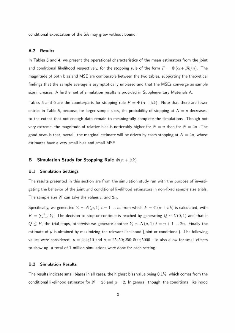
In Tables 3 and 4, we present the operational characteristics of the mean estimators from the joint
and conditional likelihood respectively, for the stopping rule of the form F = Φ (α+ βk/n). The
magnitude of both bias and MSE are comparable between the two tables, supporting the theoretical
findings that the sample average is asymptotically unbiased and that the MSEs converge as sample
size increases. A further set of simulation results is provided in Supplementary Materials A.
Tables 5 and 6 are the counterparts for stopping rule F = Φ (α+ βk). Note that there are fewer
entries in Table 5, because, for larger sample sizes, the probability of stopping at N = n decreases,
to the extent that not enough data remain to meaningfully complete the simulations. Though not
very extreme, the magnitude of relative bias is noticeably higher for N = n than for N = 2n. The
good news is that, overall, the marginal estimate will be driven by cases stopping at N = 2n, whose
estimates have a very small bias and small MSE.
B Simulation Study for Stopping Rule Φ(α + βk)
B.1 Simulation Settings
The results presented in this section are from the simulation study run with the purpose of investi-
gating the behavior of the joint and conditional likelihood estimators in non-fixed sample size trials.
The sample size N can take the values n and 2n.
Specifically, we generated Yi ∼ N(µ, 1) i = 1 . . . n, from which F = Φ (α+ βk) is calculated, with
K =∑n
i=1 Yi. The decision to stop or continue is reached by generating Q ∼ U(0, 1) and that if
Q ≤ F , the trial stops, otherwise we generate another Yi ∼ N(µ, 1) i = n + 1 . . . 2n. Finally the
estimate of µ is obtained by maximizing the relevant likelihood (joint or conditional). The following
values were considered: µ = 2; 4; 10 and n = 25; 50; 250; 500; 5000. To also allow for small effects
to show up, a total of 1 million simulations were done for each setting.
B.2 Simulation Results
The results indicate small biases in all cases, the highest bias value being 0.1%, which comes from the
conditional likelihood estimator for N = 25 and µ = 2. In general, though, the conditional likelihood
2
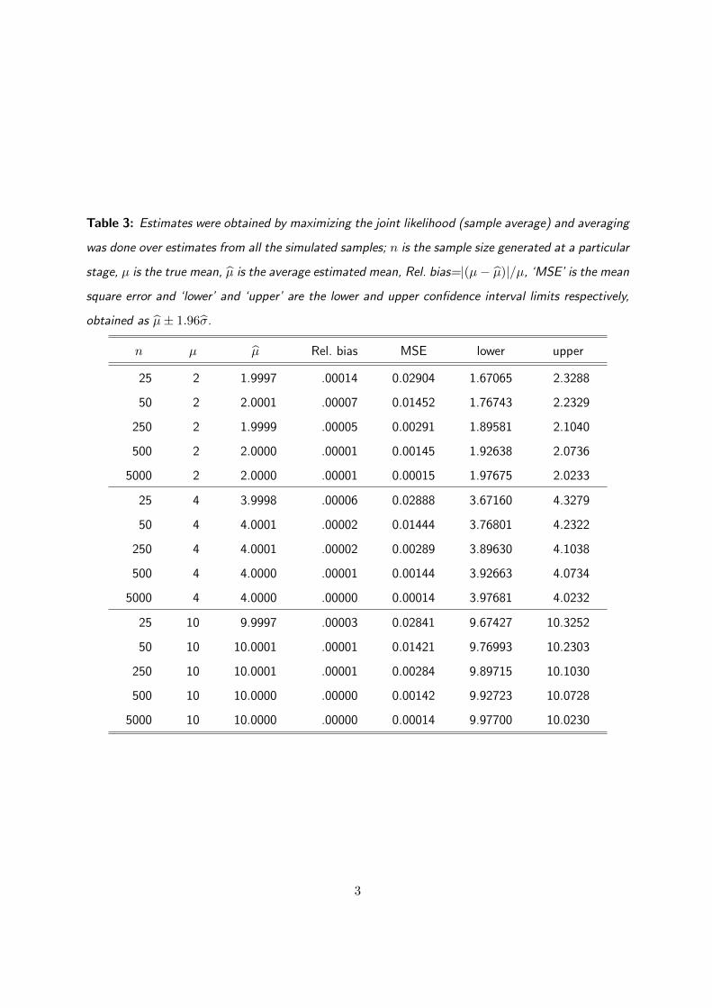
Table 3: Estimates were obtained by maximizing the joint likelihood (sample average) and averaging
was done over estimates from all the simulated samples; n is the sample size generated at a particular
stage, µ is the true mean, µ is the average estimated mean, Rel. bias=|(µ− µ)|/µ, ‘MSE’ is the mean
square error and ‘lower’ and ‘upper’ are the lower and upper confidence interval limits respectively,
obtained as µ± 1.96σ.
n µ µ Rel. bias MSE lower upper
25 2 1.9997 .00014 0.02904 1.67065 2.3288
50 2 2.0001 .00007 0.01452 1.76743 2.2329
250 2 1.9999 .00005 0.00291 1.89581 2.1040
500 2 2.0000 .00001 0.00145 1.92638 2.0736
5000 2 2.0000 .00001 0.00015 1.97675 2.0233
25 4 3.9998 .00006 0.02888 3.67160 4.3279
50 4 4.0001 .00002 0.01444 3.76801 4.2322
250 4 4.0001 .00002 0.00289 3.89630 4.1038
500 4 4.0000 .00001 0.00144 3.92663 4.0734
5000 4 4.0000 .00000 0.00014 3.97681 4.0232
25 10 9.9997 .00003 0.02841 9.67427 10.3252
50 10 10.0001 .00001 0.01421 9.76993 10.2303
250 10 10.0001 .00001 0.00284 9.89715 10.1030
500 10 10.0000 .00000 0.00142 9.92723 10.0728
5000 10 10.0000 .00000 0.00014 9.97700 10.0230
3
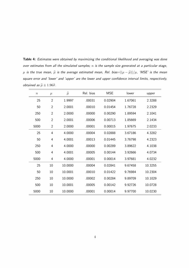
Table 4: Estimates were obtained by maximizing the conditional likelihood and averaging was done
over estimates from all the simulated samples; n is the sample size generated at a particular stage,
µ is the true mean, µ is the average estimated mean, Rel. bias=|(µ− µ)|/µ, ‘MSE’ is the mean
square error and ‘lower’ and ‘upper’ are the lower and upper confidence interval limits, respectively,
obtained as µ± 1.96σ.
n µ µ Rel. bias MSE lower upper
25 2 1.9997 .00031 0.02904 1.67061 2.3288
50 2 2.0001 .00010 0.01454 1.76728 2.2329
250 2 2.0000 .00000 0.00290 1.89594 2.1041
500 2 2.0001 .00006 0.00713 1.85669 2.1434
5000 2 2.0000 .00001 0.00015 1.97675 2.0233
25 4 4.0000 .00004 0.02888 3.67186 4.3282
50 4 4.0001 .00013 0.01445 3.76798 4.2323
250 4 4.0000 .00000 0.00289 3.89622 4.1038
500 4 4.0001 .00005 0.00144 3.92666 4.0734
5000 4 4.0000 .00001 0.00014 3.97681 4.0232
25 10 10.0000 .00004 0.02841 9.67458 10.3255
50 10 10.0001 .00010 0.01422 9.76984 10.2304
250 10 10.0000 .00002 0.00284 9.89709 10.1029
500 10 10.0001 .00005 0.00142 9.92726 10.0728
5000 10 10.0000 .00001 0.00014 9.97700 10.0230
4
Table 5: Estimates were obtained by maximizing the joint likelihood and averaging was done over
estimates from all the simulated samples where we stopped at N = n; n is the sample size generated
at a particular stage, µ is the true mean, µ is the average estimated mean, Rel. bias=|(µ− µ)|/µ,
‘MSE’ is the mean square error and ‘lower’ and ‘upper’ are the lower and upper confidence interval
limits, respectively, obtained as µ± 1.96σ.
n µ µ Rel. bias MSE lower upper
25 2 1.98573 0.00714 0.04009 1.59438 2.3771
50 2 1.95704 0.02148 0.02062 1.68982 2.2243
250 2 1.90287 0.04856 0.01343 1.77891 2.0268
25 4 3.97778 0.00555 0.04022 3.58737 4.3682
50 4 3.85891 0.03527 0.03438 3.62663 4.0912
25 10 9.97525 0.00248 0.04061 9.58325 10.3673
estimator shows little or no bias. For the sample average, comparing the overall results with the ones
conditional on sample size, reveals that the bias is slightly higher in the conditional estimates than
the marginal ones for the small sample size. The asymptotic behavior of bias is in line with theory,
given that it decreases with increasing sample size. Loss of information in the conditional estimates
is noticeable but very small in the settings studied, again in line with theory.
Details are provided in Tables 13–18.
C Simulation Study for Stopping Rule Φ(α + βk/n)
C.1 Simulation Settings
The results presented here are from a simulation study run with the purpose of investigating the
behavior of joint and conditional likelihood estimators in non-fixed sample size trials. In contrast to
Section B.1 the stopping rule is now F = Φ(α+ β kn
). All other settings are as in Section B.1.
C.2 Simulation Results
The results show small biases in all cases, the highest bias value being 0.1% which comes from the
conditional likelihood estimate for N = 25 and µ = 2, though in general the conditional likelihood
5
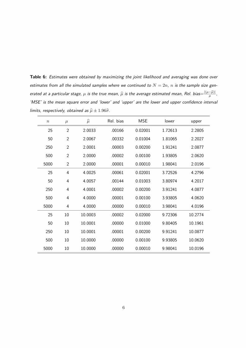
Table 6: Estimates were obtained by maximizing the joint likelihood and averaging was done over
estimates from all the simulated samples where we continued to N = 2n, n is the sample size gen-
erated at a particular stage, µ is the true mean, µ is the average estimated mean, Rel. bias= |(µ−µ)|µ ,
‘MSE’ is the mean square error and ‘lower’ and ‘upper’ are the lower and upper confidence interval
limits, respectively, obtained as µ± 1.96σ.
n µ µ Rel. bias MSE lower upper
25 2 2.0033 .00166 0.02001 1.72613 2.2805
50 2 2.0067 .00332 0.01004 1.81065 2.2027
250 2 2.0001 .00003 0.00200 1.91241 2.0877
500 2 2.0000 .00002 0.00100 1.93805 2.0620
5000 2 2.0000 .00001 0.00010 1.98041 2.0196
25 4 4.0025 .00061 0.02001 3.72526 4.2796
50 4 4.0057 .00144 0.01003 3.80974 4.2017
250 4 4.0001 .00002 0.00200 3.91241 4.0877
500 4 4.0000 .00001 0.00100 3.93805 4.0620
5000 4 4.0000 .00000 0.00010 3.98041 4.0196
25 10 10.0003 .00002 0.02000 9.72306 10.2774
50 10 10.0001 .00000 0.01000 9.80405 10.1961
250 10 10.0001 .00001 0.00200 9.91241 10.0877
500 10 10.0000 .00000 0.00100 9.93805 10.0620
5000 10 10.0000 .00000 0.00010 9.98041 10.0196
6
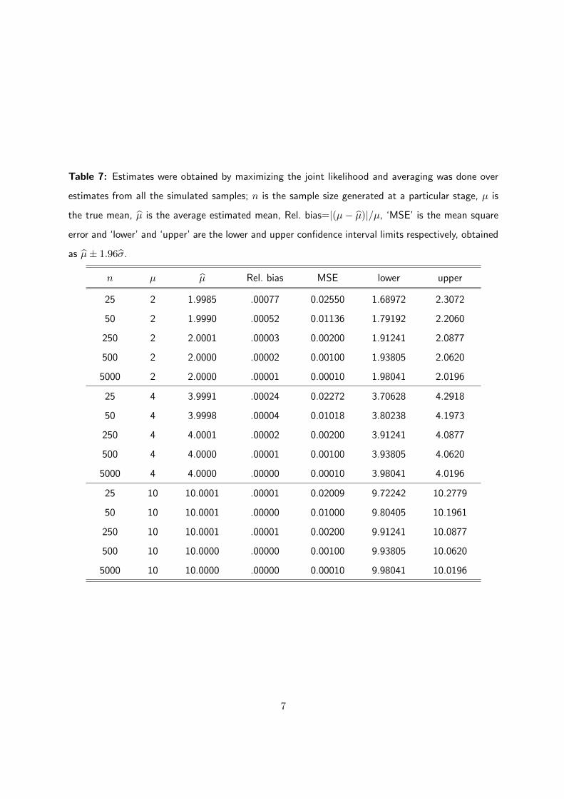
Table 7: Estimates were obtained by maximizing the joint likelihood and averaging was done over
estimates from all the simulated samples; n is the sample size generated at a particular stage, µ is
the true mean, µ is the average estimated mean, Rel. bias=|(µ− µ)|/µ, ‘MSE’ is the mean square
error and ‘lower’ and ‘upper’ are the lower and upper confidence interval limits respectively, obtained
as µ± 1.96σ.
n µ µ Rel. bias MSE lower upper
25 2 1.9985 .00077 0.02550 1.68972 2.3072
50 2 1.9990 .00052 0.01136 1.79192 2.2060
250 2 2.0001 .00003 0.00200 1.91241 2.0877
500 2 2.0000 .00002 0.00100 1.93805 2.0620
5000 2 2.0000 .00001 0.00010 1.98041 2.0196
25 4 3.9991 .00024 0.02272 3.70628 4.2918
50 4 3.9998 .00004 0.01018 3.80238 4.1973
250 4 4.0001 .00002 0.00200 3.91241 4.0877
500 4 4.0000 .00001 0.00100 3.93805 4.0620
5000 4 4.0000 .00000 0.00010 3.98041 4.0196
25 10 10.0001 .00001 0.02009 9.72242 10.2779
50 10 10.0001 .00000 0.01000 9.80405 10.1961
250 10 10.0001 .00001 0.00200 9.91241 10.0877
500 10 10.0000 .00000 0.00100 9.93805 10.0620
5000 10 10.0000 .00000 0.00010 9.98041 10.0196
7
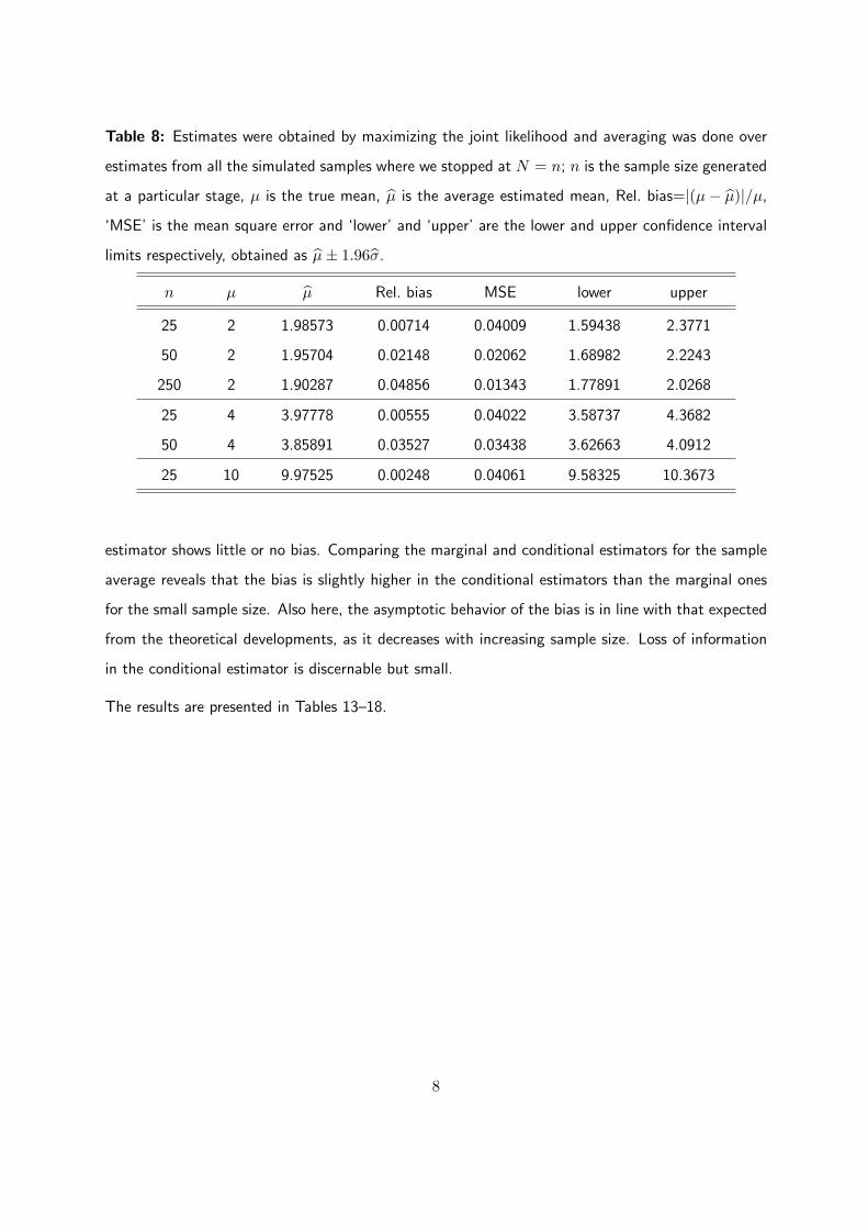
Table 8: Estimates were obtained by maximizing the joint likelihood and averaging was done over
estimates from all the simulated samples where we stopped at N = n; n is the sample size generated
at a particular stage, µ is the true mean, µ is the average estimated mean, Rel. bias=|(µ− µ)|/µ,
‘MSE’ is the mean square error and ‘lower’ and ‘upper’ are the lower and upper confidence interval
limits respectively, obtained as µ± 1.96σ.
n µ µ Rel. bias MSE lower upper
25 2 1.98573 0.00714 0.04009 1.59438 2.3771
50 2 1.95704 0.02148 0.02062 1.68982 2.2243
250 2 1.90287 0.04856 0.01343 1.77891 2.0268
25 4 3.97778 0.00555 0.04022 3.58737 4.3682
50 4 3.85891 0.03527 0.03438 3.62663 4.0912
25 10 9.97525 0.00248 0.04061 9.58325 10.3673
estimator shows little or no bias. Comparing the marginal and conditional estimators for the sample
average reveals that the bias is slightly higher in the conditional estimators than the marginal ones
for the small sample size. Also here, the asymptotic behavior of the bias is in line with that expected
from the theoretical developments, as it decreases with increasing sample size. Loss of information
in the conditional estimator is discernable but small.
The results are presented in Tables 13–18.
8

Table 9: Estimates were obtained by maximizing the joint likelihood and averaging was done over es-
timates from all the simulated samples where we continued to N = 2n, n is the sample size generated
at a particular stage, µ is the true mean, µ is the average estimated mean, Rel. bias=|(µ− µ)|/µ,
‘MSE’ is the mean square error and ‘lower’ and ‘upper’ are the lower and upper confidence interval
limits respectively, obtained as µ± 1.96σ.
n µ µ Rel. bias MSE lower upper
25 2 2.0033 .00166 0.02001 1.72613 2.2805
50 2 2.0067 .00332 0.01004 1.81065 2.2027
250 2 2.0001 .00003 0.00200 1.91241 2.0877
500 2 2.0000 .00002 0.00100 1.93805 2.0620
5000 2 2.0000 .00001 0.00010 1.98041 2.0196
25 4 4.0025 .00061 0.02001 3.72526 4.2796
50 4 4.0057 .00144 0.01003 3.80974 4.2017
250 4 4.0001 .00002 0.00200 3.91241 4.0877
500 4 4.0000 .00001 0.00100 3.93805 4.0620
5000 4 4.0000 .00000 0.00010 3.98041 4.0196
25 10 10.0003 .00002 0.02000 9.72306 10.2774
50 10 10.0001 .00000 0.01000 9.80405 10.1961
250 10 10.0001 .00001 0.00200 9.91241 10.0877
500 10 10.0000 .00000 0.00100 9.93805 10.0620
5000 10 10.0000 .00000 0.00010 9.98041 10.0196
9
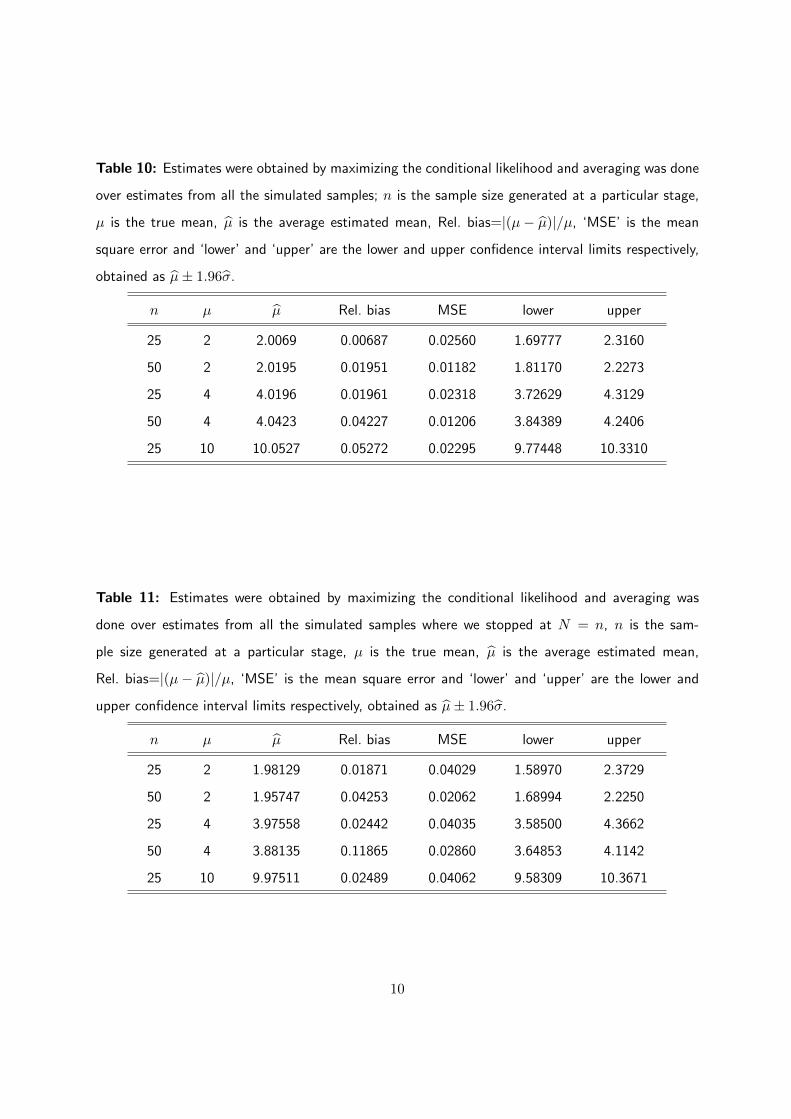
Table 10: Estimates were obtained by maximizing the conditional likelihood and averaging was done
over estimates from all the simulated samples; n is the sample size generated at a particular stage,
µ is the true mean, µ is the average estimated mean, Rel. bias=|(µ− µ)|/µ, ‘MSE’ is the mean
square error and ‘lower’ and ‘upper’ are the lower and upper confidence interval limits respectively,
obtained as µ± 1.96σ.
n µ µ Rel. bias MSE lower upper
25 2 2.0069 0.00687 0.02560 1.69777 2.3160
50 2 2.0195 0.01951 0.01182 1.81170 2.2273
25 4 4.0196 0.01961 0.02318 3.72629 4.3129
50 4 4.0423 0.04227 0.01206 3.84389 4.2406
25 10 10.0527 0.05272 0.02295 9.77448 10.3310
Table 11: Estimates were obtained by maximizing the conditional likelihood and averaging was
done over estimates from all the simulated samples where we stopped at N = n, n is the sam-
ple size generated at a particular stage, µ is the true mean, µ is the average estimated mean,
Rel. bias=|(µ− µ)|/µ, ‘MSE’ is the mean square error and ‘lower’ and ‘upper’ are the lower and
upper confidence interval limits respectively, obtained as µ± 1.96σ.
n µ µ Rel. bias MSE lower upper
25 2 1.98129 0.01871 0.04029 1.58970 2.3729
50 2 1.95747 0.04253 0.02062 1.68994 2.2250
25 4 3.97558 0.02442 0.04035 3.58500 4.3662
50 4 3.88135 0.11865 0.02860 3.64853 4.1142
25 10 9.97511 0.02489 0.04062 9.58309 10.3671
10
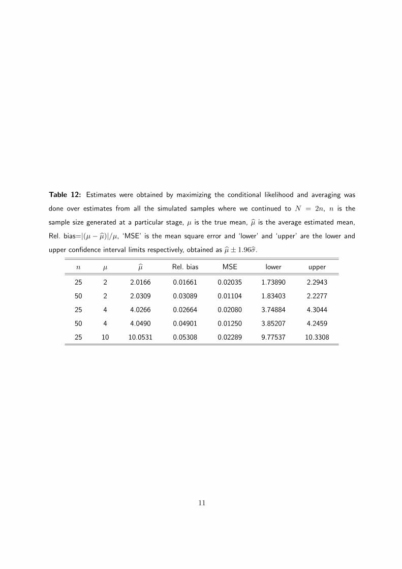
Table 12: Estimates were obtained by maximizing the conditional likelihood and averaging was
done over estimates from all the simulated samples where we continued to N = 2n, n is the
sample size generated at a particular stage, µ is the true mean, µ is the average estimated mean,
Rel. bias=|(µ− µ)|/µ, ‘MSE’ is the mean square error and ‘lower’ and ‘upper’ are the lower and
upper confidence interval limits respectively, obtained as µ± 1.96σ.
n µ µ Rel. bias MSE lower upper
25 2 2.0166 0.01661 0.02035 1.73890 2.2943
50 2 2.0309 0.03089 0.01104 1.83403 2.2277
25 4 4.0266 0.02664 0.02080 3.74884 4.3044
50 4 4.0490 0.04901 0.01250 3.85207 4.2459
25 10 10.0531 0.05308 0.02289 9.77537 10.3308
11
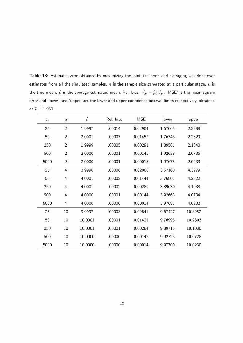
Table 13: Estimates were obtained by maximizing the joint likelihood and averaging was done over
estimates from all the simulated samples, n is the sample size generated at a particular stage, µ is
the true mean, µ is the average estimated mean, Rel. bias=|(µ− µ)|/µ, ‘MSE’ is the mean square
error and ‘lower’ and ‘upper’ are the lower and upper confidence interval limits respectively, obtained
as µ± 1.96σ.
n µ µ Rel. bias MSE lower upper
25 2 1.9997 .00014 0.02904 1.67065 2.3288
50 2 2.0001 .00007 0.01452 1.76743 2.2329
250 2 1.9999 .00005 0.00291 1.89581 2.1040
500 2 2.0000 .00001 0.00145 1.92638 2.0736
5000 2 2.0000 .00001 0.00015 1.97675 2.0233
25 4 3.9998 .00006 0.02888 3.67160 4.3279
50 4 4.0001 .00002 0.01444 3.76801 4.2322
250 4 4.0001 .00002 0.00289 3.89630 4.1038
500 4 4.0000 .00001 0.00144 3.92663 4.0734
5000 4 4.0000 .00000 0.00014 3.97681 4.0232
25 10 9.9997 .00003 0.02841 9.67427 10.3252
50 10 10.0001 .00001 0.01421 9.76993 10.2303
250 10 10.0001 .00001 0.00284 9.89715 10.1030
500 10 10.0000 .00000 0.00142 9.92723 10.0728
5000 10 10.0000 .00000 0.00014 9.97700 10.0230
12
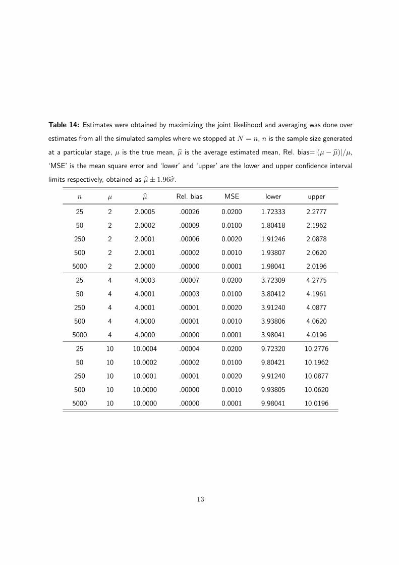
Table 14: Estimates were obtained by maximizing the joint likelihood and averaging was done over
estimates from all the simulated samples where we stopped at N = n, n is the sample size generated
at a particular stage, µ is the true mean, µ is the average estimated mean, Rel. bias=|(µ− µ)|/µ,
‘MSE’ is the mean square error and ‘lower’ and ‘upper’ are the lower and upper confidence interval
limits respectively, obtained as µ± 1.96σ.
n µ µ Rel. bias MSE lower upper
25 2 2.0005 .00026 0.0200 1.72333 2.2777
50 2 2.0002 .00009 0.0100 1.80418 2.1962
250 2 2.0001 .00006 0.0020 1.91246 2.0878
500 2 2.0001 .00002 0.0010 1.93807 2.0620
5000 2 2.0000 .00000 0.0001 1.98041 2.0196
25 4 4.0003 .00007 0.0200 3.72309 4.2775
50 4 4.0001 .00003 0.0100 3.80412 4.1961
250 4 4.0001 .00001 0.0020 3.91240 4.0877
500 4 4.0000 .00001 0.0010 3.93806 4.0620
5000 4 4.0000 .00000 0.0001 3.98041 4.0196
25 10 10.0004 .00004 0.0200 9.72320 10.2776
50 10 10.0002 .00002 0.0100 9.80421 10.1962
250 10 10.0001 .00001 0.0020 9.91240 10.0877
500 10 10.0000 .00000 0.0010 9.93805 10.0620
5000 10 10.0000 .00000 0.0001 9.98041 10.0196
13

Table 15: Estimates were obtained by maximizing the joint likelihood and averaging was done over
estimates from all the simulated samples where we continued to N = 2n, n is the sample size gener-
ated at a particular stage, µ is the true mean, µ is the average estimated mean, Rel. bias=|(µ− µ)|/µ,
‘MSE’ is the mean square error and ‘lower’ and ‘upper’ are the lower and upper confidence interval
limits respectively, obtained as µ± 1.96σ.
n µ µ Rel. bias MSE lower upper
25 2 1.9994 .00031 0.03291 1.64807 2.3507
50 2 2.0001 .00006 0.01646 1.75168 2.2486
250 2 1.9998 .00009 0.00330 1.88866 2.1110
500 2 2.0000 .00002 0.00165 1.92137 2.0786
5000 2 2.0000 .00001 0.00016 1.97518 2.0249
25 4 3.9995 .00012 0.03287 3.64846 4.3506
50 4 4.0001 .00002 0.01643 3.75188 4.2483
250 4 4.0001 .00002 0.00328 3.88910 4.1111
500 4 4.0000 .00000 0.00164 3.92154 4.0785
5000 4 4.0000 .00000 0.00016 3.97521 4.0248
25 10 9.9994 .00006 0.03265 9.64959 10.3492
50 10 10.0001 .00001 0.01634 9.75262 10.2475
250 10 10.0001 .00001 0.00327 9.88944 10.1107
500 10 10.0000 .00000 0.00163 9.92178 10.0783
5000 10 10.0000 .00000 0.00016 9.97529 10.0248
14

Table 16: Estimates were obtained by maximizing the conditional likelihood and averaging was done
over estimates from all the simulated samples; n is the sample size generated at a particular stage,
µ is the true mean, µ is the average estimated mean, Rel. bias=|(µ− µ)|/µ, ‘MSE’ is the mean
square error and ‘lower’ and ‘upper’ are the lower and upper confidence interval limits respectively,
obtained as µ± 1.96σ.
n µ µ Rel. bias MSE lower upper
25 2 1.9997 .00031 0.02904 1.67061 2.3288
50 2 2.0001 .00010 0.01454 1.76728 2.2329
250 2 2.0000 .00000 0.00290 1.89594 2.1041
500 2 2.0001 .00006 0.00713 1.85669 2.1434
5000 2 2.0000 .00001 0.00015 1.97675 2.0233
25 4 4.0000 .00004 0.02888 3.67186 4.3282
50 4 4.0001 .00013 0.01445 3.76798 4.2323
250 4 4.0000 .00000 0.00289 3.89622 4.1038
500 4 4.0001 .00005 0.00144 3.92666 4.0734
5000 4 4.0000 .00001 0.00014 3.97681 4.0232
25 10 10.0000 .00004 0.02841 9.67458 10.3255
50 10 10.0001 .00010 0.01422 9.76984 10.2304
250 10 10.0000 .00002 0.00284 9.89709 10.1029
500 10 10.0001 .00005 0.00142 9.92726 10.0728
5000 10 10.0000 .00001 0.00014 9.97700 10.0230
15
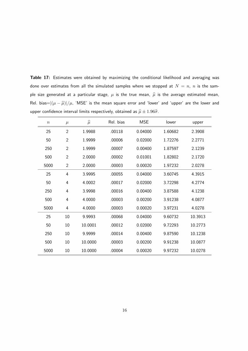
Table 17: Estimates were obtained by maximizing the conditional likelihood and averaging was
done over estimates from all the simulated samples where we stopped at N = n, n is the sam-
ple size generated at a particular stage, µ is the true mean, µ is the average estimated mean,
Rel. bias=|(µ− µ)|/µ, ‘MSE’ is the mean square error and ‘lower’ and ‘upper’ are the lower and
upper confidence interval limits respectively, obtained as µ± 1.96σ.
n µ µ Rel. bias MSE lower upper
25 2 1.9988 .00118 0.04000 1.60682 2.3908
50 2 1.9999 .00006 0.02000 1.72276 2.2771
250 2 1.9999 .00007 0.00400 1.87597 2.1239
500 2 2.0000 .00002 0.01001 1.82802 2.1720
5000 2 2.0000 .00003 0.00020 1.97232 2.0278
25 4 3.9995 .00055 0.04000 3.60745 4.3915
50 4 4.0002 .00017 0.02000 3.72298 4.2774
250 4 3.9998 .00016 0.00400 3.87588 4.1238
500 4 4.0000 .00003 0.00200 3.91238 4.0877
5000 4 4.0000 .00003 0.00020 3.97231 4.0278
25 10 9.9993 .00068 0.04000 9.60732 10.3913
50 10 10.0001 .00012 0.02000 9.72293 10.2773
250 10 9.9999 .00014 0.00400 9.87590 10.1238
500 10 10.0000 .00003 0.00200 9.91238 10.0877
5000 10 10.0000 .00004 0.00020 9.97232 10.0278
16
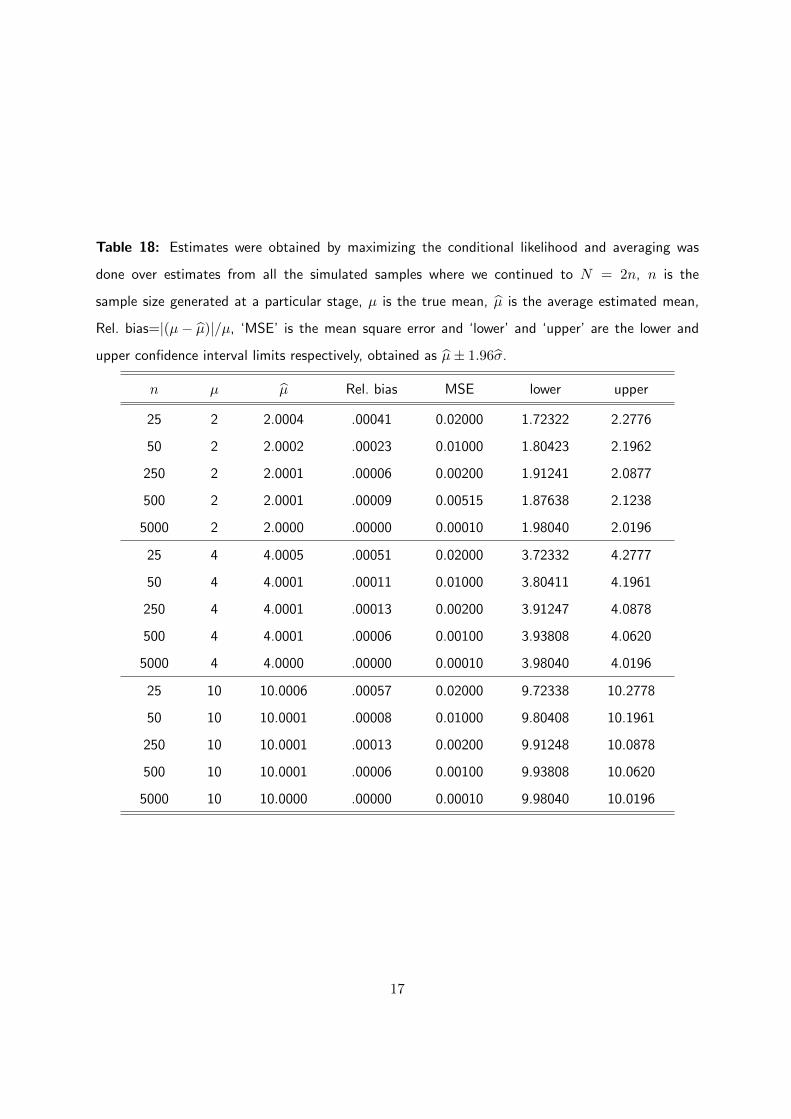
Table 18: Estimates were obtained by maximizing the conditional likelihood and averaging was
done over estimates from all the simulated samples where we continued to N = 2n, n is the
sample size generated at a particular stage, µ is the true mean, µ is the average estimated mean,
Rel. bias=|(µ− µ)|/µ, ‘MSE’ is the mean square error and ‘lower’ and ‘upper’ are the lower and
upper confidence interval limits respectively, obtained as µ± 1.96σ.
n µ µ Rel. bias MSE lower upper
25 2 2.0004 .00041 0.02000 1.72322 2.2776
50 2 2.0002 .00023 0.01000 1.80423 2.1962
250 2 2.0001 .00006 0.00200 1.91241 2.0877
500 2 2.0001 .00009 0.00515 1.87638 2.1238
5000 2 2.0000 .00000 0.00010 1.98040 2.0196
25 4 4.0005 .00051 0.02000 3.72332 4.2777
50 4 4.0001 .00011 0.01000 3.80411 4.1961
250 4 4.0001 .00013 0.00200 3.91247 4.0878
500 4 4.0001 .00006 0.00100 3.93808 4.0620
5000 4 4.0000 .00000 0.00010 3.98040 4.0196
25 10 10.0006 .00057 0.02000 9.72338 10.2778
50 10 10.0001 .00008 0.01000 9.80408 10.1961
250 10 10.0001 .00013 0.00200 9.91248 10.0878
500 10 10.0001 .00006 0.00100 9.93808 10.0620
5000 10 10.0000 .00000 0.00010 9.98040 10.0196
17