ESTIMATING WITH CONFIDENCE - DXC Technologyassets1.csc.com/innovation/downloads/Estimating_with_Confidence.… · 2 ESTIMATING WITH CONF IDENCE chicken and egg thing. Let’s ignore

CSC PAPERS Copyright © 2013 Computer Sciences Corporation. All rights reserved.

ESTIMATING WITH CONFIDENCE

ABSTRACT With the increasing prevalence of fixed-price contracts, the need to accurately, estimate IT projects is greater than ever. In today’s economy, we cannot afford to get it wrong. The purpose of this paper is to demonstrate an estimation approach that increases the chances for successful estimates of project effort and schedule. Such estimates are subject to large amounts of inherent estimation risk, defined as the probability that the project will overrun the estimate. Estimators can identify, measure, and adjust for this inherent risk using a risk-adjusted estimation approach. The result is an estimate that meets specific estimation risk objectives. We explain the approach using an ongoing example of how to derive internally and mutually consistent, risk-adjusted effort and schedule estimates, and illustrate the example with screen shots from the following tools:

• Excel, the standard spreadsheet product from Microsoft

• RiskAMP, a Monte Carlo simulation add-in to Excel from Structured Data, LLC

• Risk-Adjustment Allocation Tool, a custom Excel spreadsheet tool

• Project, the standard scheduling product from Microsoft

• @Risk for Project, a Monte Carlo simulation add-in to Project from Palisade Corporation

Keywords: Project Estimation, Risk-adjusted Estimate, Effort Estimate, Schedule Estimate, Monte Carlo Simulation, Risk, RiskAMP, @Risk for Project THE PROBLEM WITH ESTIMATES The problem with estimates is you just can’t trust them. How can you when much of the time they don’t seem to work out very well? We assign a bevy of experts to the task of estimating a project, compare to historical data, use sophisticated software, and the project still overruns the estimate. What is the problem here?

Sometimes the problem is that the estimators fail to account for all of the work that the project will perform. Other times, the problem is that the project performs different work, performs the work differently, or is less productive than was estimated. It’s kind of a

Yale Esrock

CSC

[email protected]

CSC Papers

2013

2


chicken and egg thing. Let’s ignore this for the moment, however, and assume that the estimate does, in fact, cover the appropriate work. Still, we often find that there are overruns. Where do we go wrong? A big part of the problem is that we tend to ignore the fundamental nature of estimates. A project estimate is a forecast of what is going to happen in the future. The future is always uncertain, and estimates, in turn, are inherently uncertain. If estimates were not uncertain they wouldn’t be estimates! Yet, we often ignore the crucial aspect of uncertainty when we derive estimates.

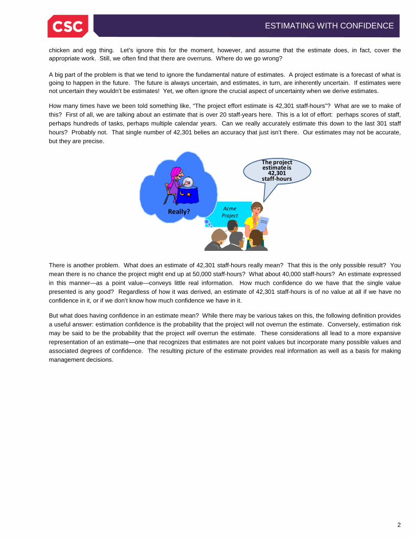
How many times have we been told something like, “The project effort estimate is 42,301 staff-hours”? What are we to make of this? First of all, we are talking about an estimate that is over 20 staff-years here. This is a lot of effort: perhaps scores of staff, perhaps hundreds of tasks, perhaps multiple calendar years. Can we really accurately estimate this down to the last 301 staff hours? Probably not. That single number of 42,301 belies an accuracy that just isn’t there. Our estimates may not be accurate, but they are precise.

There is another problem. What does an estimate of 42,301 staff-hours really mean? That this is the only possible result? You mean there is no chance the project might end up at 50,000 staff-hours? What about 40,000 staff-hours? An estimate expressed in this manner—as a point value—conveys little real information. How much confidence do we have that the single value presented is any good? Regardless of how it was derived, an estimate of 42,301 staff-hours is of no value at all if we have no confidence in it, or if we don’t know how much confidence we have in it.

But what does having confidence in an estimate mean? While there may be various takes on this, the following definition provides a useful answer: estimation confidence is the probability that the project will not overrun the estimate. Conversely, estimation risk may be said to be the probability that the project will overrun the estimate. These considerations all lead to a more expansive representation of an estimate—one that recognizes that estimates are not point values but incorporate many possible values and associated degrees of confidence. The resulting picture of the estimate provides real information as well as a basis for making management decisions.

AcmeProject

The project estimate is

42,301staff-hours

Really?

3


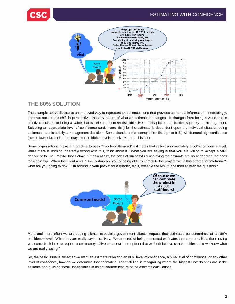
THE 80% SOLUTION The example above illustrates an improved way to represent an estimate—one that provides some real information. Interestingly, once we accept this shift in perspective, the very nature of what an estimate is changes. It changes from being a value that is strictly calculated to being a value that is selected to meet risk objectives. This places the burden squarely on management. Selecting an appropriate level of confidence (and, hence risk) for the estimate is dependent upon the individual situation being estimated, and is strictly a management decision. Some situations (for example firm fixed price bids) will demand high confidence (hence low risk), and others may tolerate higher levels of risk. More on this later.

Some organizations make it a practice to seek “middle-of the-road” estimates that reflect approximately a 50% confidence level. While there is nothing inherently wrong with this, think about it. What you are saying is that you are willing to accept a 50% chance of failure. Maybe that’s okay, but essentially, the odds of successfully achieving the estimate are no better than the odds for a coin flip. When the client asks, “How certain are you of being able to complete the project within this effort and timeframe?” what are you going to do? Fish around in your pocket for a quarter, flip it, observe the result, and then answer the question?

More and more often we are seeing clients, especially government clients, request that estimates be determined at an 80% confidence level. What they are really saying is, “Hey. We are tired of being presented estimates that are unrealistic, then having you come back later to request more money. Give us an estimate upfront that we both believe can be achieved so we know what we are really facing.”

So, the basic issue is, whether we want an estimate reflecting an 80% level of confidence, a 50% level of confidence, or any other level of confidence, how do we determine that estimate? The trick lies in recognizing where the biggest uncertainties are in the estimate and building these uncertainties in as an inherent feature of the estimate calculations.

AcmeProject

The project estimateranges from a low of 40,123 to a high

of 50,061 staff-hours.The mean estimate is 46,201.

Probability of achieving our targetof 42,301 is only 8%.

To be 80% confident, the estimate should be 47,194 staff-hours.

40K 45K 50K

EFFORT (STAFF-HOURS)

.10

.20

.30

.40

.50

.60

.70

.80

.901.00

xx

x

x

xx

x

x

x

PRO

BABI

LITY

xx

x

x

Aha!

TARGET42,301

47,194

.08

AcmeProject

Of course we can complete the project in

42,301staff-hours!

Come on heads!

4


RECOGNIZING UNCERTAINTY Incorporating uncertainty starts by identifying those components of the estimate for which we have the most doubt. Not all parts of the estimate will be uncertain. We may have a lot of history, a lot of experience, or just a lot of confidence in some parts. Maybe some parts are small or relatively simple to perform. Some may essentially be constant as, for instance, time-boxed tasks.

There will likely be other parts of the estimate, however, about which we feel a bit queasy. Maybe these parts are large and complex, maybe we don’t have experience or history with them, or maybe we just don’t have very much information about what they actually are. These parts of the estimate should be highlighted and treated differently

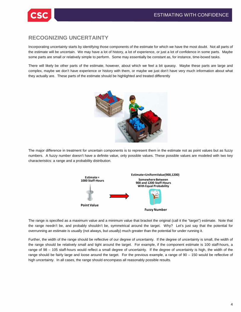
The major difference in treatment for uncertain components is to represent them in the estimate not as point values but as fuzzy numbers. A fuzzy number doesn’t have a definite value, only possible values. These possible values are modeled with two key characteristics: a range and a probability distribution.

The range is specified as a maximum value and a minimum value that bracket the original (call it the “target”) estimate. Note that the range needn’t be, and probably shouldn’t be, symmetrical around the target. Why? Let’s just say that the potential for overrunning an estimate is usually (not always, but usually) much greater than the potential for under running it.

Further, the width of the range should be reflective of our degree of uncertainty. If the degree of uncertainty is small, the width of the range should be relatively small and tight around the target. For example, if the component estimate is 100 staff-hours, a range of 98 – 105 staff-hours would reflect a small degree of uncertainty. If the degree of uncertainty is high, the width of the range should be fairly large and loose around the target. For the previous example, a range of 90 – 150 would be reflective of high uncertainty. In all cases, the range should encompass all reasonably possible results.

Estimate = 1000 Staff-Hours

Fuzzy NumberPoint Value

Somewhere Between900 and 1200 Staff-Hours

With Equal Probability

Estimate=UniformValue(900,1200)

5


A Low Uncertainty Range A High Uncertainty Range A fuzzy number can assume any value within its specified range. The second characteristic of fuzzy numbers—the probability distribution—helps determine which of these values will actually be assumed. The probability distribution is a mathematical function often stated in terms of the estimate’s minimum, maximum, and target values. It relates each value in the range to the probability of not overrunning that value. In accordance with the probability distribution function (actually an inverse cumulative probability density function, but don’t worry about that), the probability of achieving the minimum value is 0%. The probability of achieving the maximum value is 100%. The probability of achieving any other value within the estimate range is between 0% and 100% and is computed by the function. Conversely, we can use the mathematical function to determine what value for the estimate corresponds to any given probability for achieving that value.

SIMULATING THE ESTIMATE Now comes the fun part—simulating the estimate. What is simulation, and what do we mean by simulating the estimate? Simulation is the process of modeling something, then performing virtual experiments on the model to better understand its behavior under varying conditions. While models can sometimes be physical things, now days they are usually mathematical. When we simulate an estimate such as an effort estimate, we use a technique known as Monte Carlo Simulation to gain increased understanding and insight into the possible results that can occur given the uncertainty embodied in the fuzzy numbers. Why is it called Monte Carlo? – because it is based upon probabilities, in much the same manner as any game of chance in a casino.

The estimate simulation model comprises the mathematical relationships (inclusive of fuzzy numbers) from which the estimate is computed. An experiment consists of randomly generating probabilities to select possible values for each fuzzy estimation parameter, then using those values to see what the result (e.g. total effort) turns out to be. Of course, this is strictly a random outcome within the possible outcomes allowed by our fuzzy numbers. If any of the random selections happened to be different, so would the final outcome. So the experiment is repeated—perhaps thousands of times—to generate an entire gamut of possible results for the estimate.

Quiet!Estimate Simulation Team at Work

6


This is significant. The result set produced by the simulation is a virtual history that provides a “window to the future”. Consider this analogy. Suppose we have an historical database consisting of 100 projects very similar to the one we are estimating. We can sort total effort for these projects from low to high and use the sorted set to analyze our estimate. Want to know the probability our estimate will not be overrun? If there are 40 projects in the history with lower total effort than our estimate, then our degree of confidence is 40%. Want to know what the estimate should be if we want 80% confidence? Find the effort for the 80th project in the sorted history.

The value of historical data is well-known as an aid to estimation. But what if we have no such history? No sweat! The simulation result set provides a virtual history that, although it is based on hypothetical and not actual project results, can be used in the exact same manner. By sorting the simulation result set from low to high, the same types of comparisons can be made. This is a window to the future because it allows us to gauge the validity of our estimate before the project begins, and provides guidance for how to modify (i.e. risk-adjust) the estimate to a value having greater confidence.

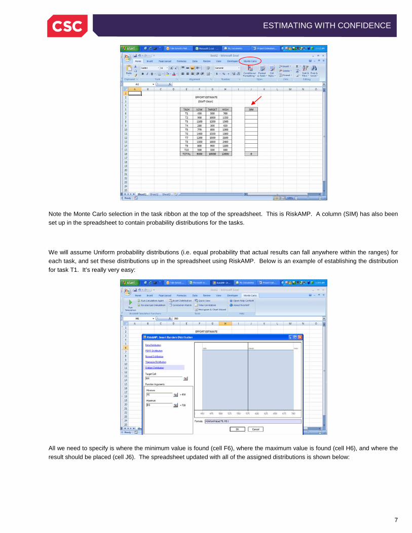
A SIMPLE EFFORT ESTIMATION EXAMPLE Let’s look at a simple example that illustrates what we’ve been talking about. We’ll use a bottom-up estimate consisting of 10 tasks totaling 10,000 staff-hours. Suppose all of the tasks are uncertain and are assigned ranges. We can simulate this estimate by setting it up in Excel and using a Monte Carlo Excel add-in. The following illustration uses the RiskAMP add-in from Structured Data, LLC:

Professor von MonteCarlo

Estimate SimulationExperiments in Progress

ESTIMATE SIMULATION

FUTUREPROJECT RESULTS

“WIN

DOW

TO THE FUTURE”

SIMULATIONRESULTS

7


Note the Monte Carlo selection in the task ribbon at the top of the spreadsheet. This is RiskAMP. A column (SIM) has also been set up in the spreadsheet to contain probability distributions for the tasks.

We will assume Uniform probability distributions (i.e. equal probability that actual results can fall anywhere within the ranges) for each task, and set these distributions up in the spreadsheet using RiskAMP. Below is an example of establishing the distribution for task T1. It’s really very easy:

All we need to specify is where the minimum value is found (cell F6), where the maximum value is found (cell H6), and where the result should be placed (cell J6). The spreadsheet updated with all of the assigned distributions is shown below:

8


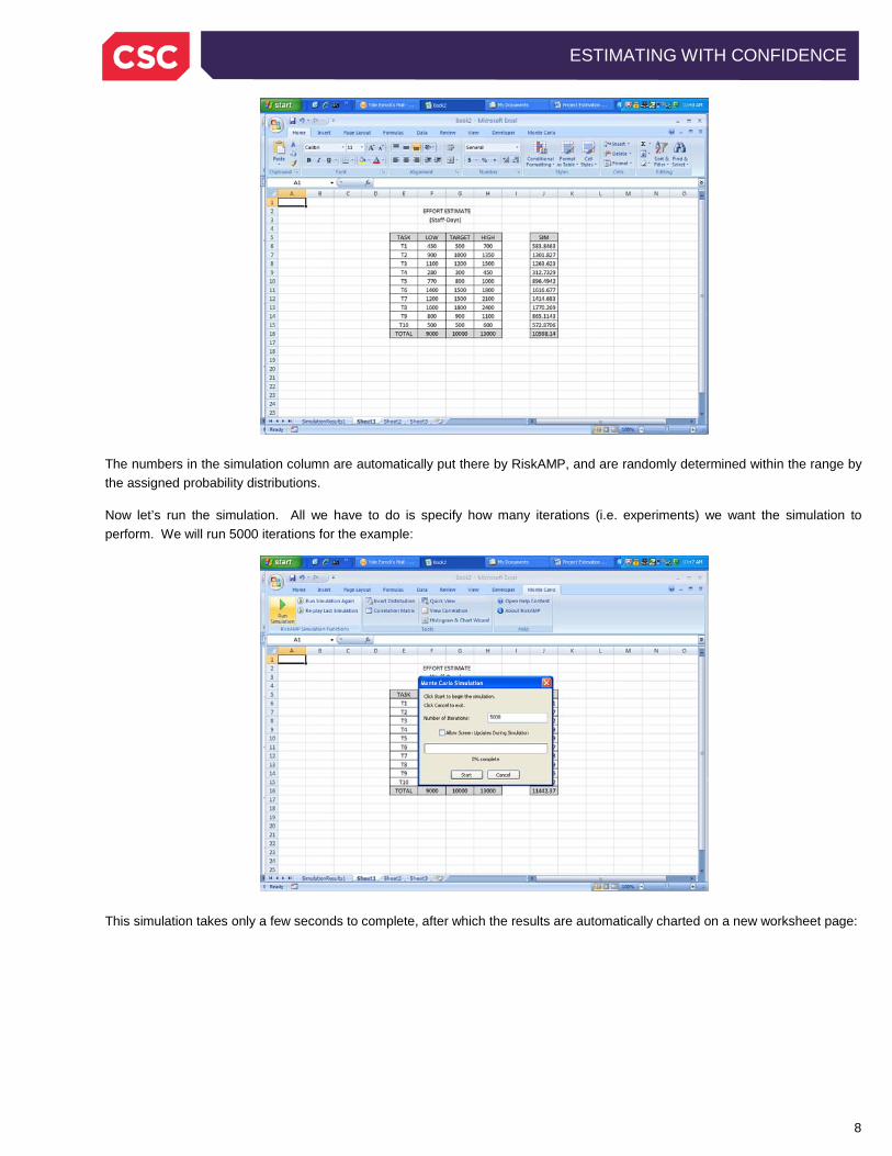
The numbers in the simulation column are automatically put there by RiskAMP, and are randomly determined within the range by the assigned probability distributions.

Now let’s run the simulation. All we have to do is specify how many iterations (i.e. experiments) we want the simulation to perform. We will run 5000 iterations for the example:

This simulation takes only a few seconds to complete, after which the results are automatically charted on a new worksheet page:

9


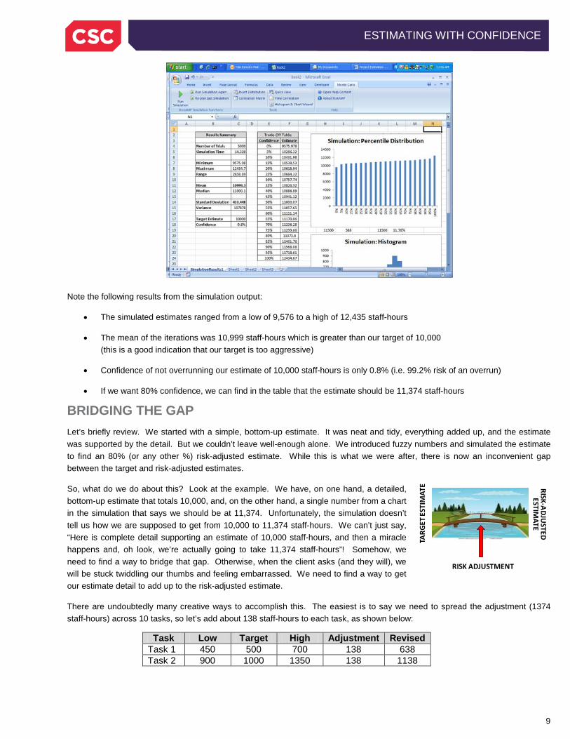
Note the following results from the simulation output:

• The simulated estimates ranged from a low of 9,576 to a high of 12,435 staff-hours

• The mean of the iterations was 10,999 staff-hours which is greater than our target of 10,000 (this is a good indication that our target is too aggressive)

• Confidence of not overrunning our estimate of 10,000 staff-hours is only 0.8% (i.e. 99.2% risk of an overrun)

• If we want 80% confidence, we can find in the table that the estimate should be 11,374 staff-hours

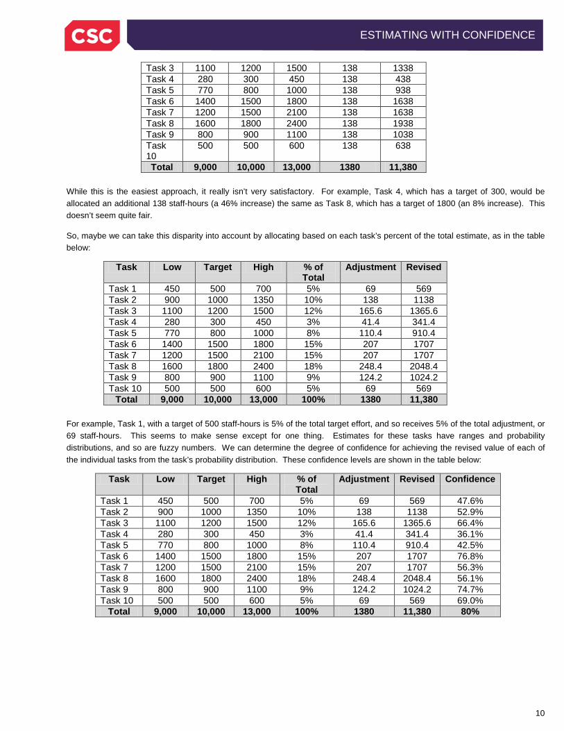
BRIDGING THE GAP Let’s briefly review. We started with a simple, bottom-up estimate. It was neat and tidy, everything added up, and the estimate was supported by the detail. But we couldn’t leave well-enough alone. We introduced fuzzy numbers and simulated the estimate to find an 80% (or any other %) risk-adjusted estimate. While this is what we were after, there is now an inconvenient gap between the target and risk-adjusted estimates.

So, what do we do about this? Look at the example. We have, on one hand, a detailed, bottom-up estimate that totals 10,000, and, on the other hand, a single number from a chart in the simulation that says we should be at 11,374. Unfortunately, the simulation doesn’t tell us how we are supposed to get from 10,000 to 11,374 staff-hours. We can’t just say, “Here is complete detail supporting an estimate of 10,000 staff-hours, and then a miracle happens and, oh look, we’re actually going to take 11,374 staff-hours”! Somehow, we need to find a way to bridge that gap. Otherwise, when the client asks (and they will), we will be stuck twiddling our thumbs and feeling embarrassed. We need to find a way to get our estimate detail to add up to the risk-adjusted estimate.

There are undoubtedly many creative ways to accomplish this. The easiest is to say we need to spread the adjustment (1374 staff-hours) across 10 tasks, so let’s add about 138 staff-hours to each task, as shown below:

Task Low Target High Adjustment Revised Task 1 450 500 700 138 638 Task 2 900 1000 1350 138 1138

TARG

ET ES

TIM

ATE RISK-ADJU

STEDESTIM

ATE

RISK ADJUSTMENT

10


Task 3 1100 1200 1500 138 1338 Task 4 280 300 450 138 438 Task 5 770 800 1000 138 938 Task 6 1400 1500 1800 138 1638 Task 7 1200 1500 2100 138 1638 Task 8 1600 1800 2400 138 1938 Task 9 800 900 1100 138 1038 Task 10

500 500 600 138 638

Total 9,000 10,000 13,000 1380 11,380 While this is the easiest approach, it really isn’t very satisfactory. For example, Task 4, which has a target of 300, would be allocated an additional 138 staff-hours (a 46% increase) the same as Task 8, which has a target of 1800 (an 8% increase). This doesn’t seem quite fair.

So, maybe we can take this disparity into account by allocating based on each task’s percent of the total estimate, as in the table below:

Task Low Target High % of Total

Adjustment Revised

Task 1 450 500 700 5% 69 569 Task 2 900 1000 1350 10% 138 1138 Task 3 1100 1200 1500 12% 165.6 1365.6 Task 4 280 300 450 3% 41.4 341.4 Task 5 770 800 1000 8% 110.4 910.4 Task 6 1400 1500 1800 15% 207 1707 Task 7 1200 1500 2100 15% 207 1707 Task 8 1600 1800 2400 18% 248.4 2048.4 Task 9 800 900 1100 9% 124.2 1024.2 Task 10 500 500 600 5% 69 569

Total 9,000 10,000 13,000 100% 1380 11,380 For example, Task 1, with a target of 500 staff-hours is 5% of the total target effort, and so receives 5% of the total adjustment, or 69 staff-hours. This seems to make sense except for one thing. Estimates for these tasks have ranges and probability distributions, and so are fuzzy numbers. We can determine the degree of confidence for achieving the revised value of each of the individual tasks from the task’s probability distribution. These confidence levels are shown in the table below:

Task Low Target High % of Total

Adjustment Revised Confidence

Task 1 450 500 700 5% 69 569 47.6% Task 2 900 1000 1350 10% 138 1138 52.9% Task 3 1100 1200 1500 12% 165.6 1365.6 66.4% Task 4 280 300 450 3% 41.4 341.4 36.1% Task 5 770 800 1000 8% 110.4 910.4 42.5% Task 6 1400 1500 1800 15% 207 1707 76.8% Task 7 1200 1500 2100 15% 207 1707 56.3% Task 8 1600 1800 2400 18% 248.4 2048.4 56.1% Task 9 800 900 1100 9% 124.2 1024.2 74.7% Task 10 500 500 600 5% 69 569 69.0%

Total 9,000 10,000 13,000 100% 1380 11,380 80%

11


Notice that confidence in achieving the revised estimate for each task varies, from a high of about 77% for Task 6 to a low of about 36% for Task 4. (It is also possible when using this method, though it doesn’t occur in this example, that the revised value for a task estimate exceeds the high value of the task’s range, which is a contradictory situation.)

Is there yet a better way to allocate the adjustment amount to the tasks? Again it doesn’t seem fair that some tasks should have very high confidence levels while others have low confidence levels.1

Task

What if we could make the confidence level for all tasks the same? It turns out, we can. What’s more, the interesting thing is that we can achieve an 80% confidence level for the overall estimate with less than 80% confidence for achieving the individual task estimates. This is illustrated in the table below:

Low Target High Confidence Adjustment Revised Task 1 450 500 700 59.5% 98.8 598.8 Task 2 900 1000 1350 59.5% 167.8 1167.8 Task 3 1100 1200 1500 59.5% 138.0 1338.0 Task 4 280 300 450 59.5% 81.2 381.2 Task 5 770 800 1000 59.5% 106.9 906.9 Task 6 1400 1500 1800 59.5% 138.0 1638.0 Task 7 1200 1500 2100 59.5% 235.5 1735.5 Task 8 1600 1800 2400 59.5% 276.0 2076.0 Task 9 800 900 1100 59.5% 78.5 978.5 Task 10 500 500 600 59.5% 59.5 559.5

Total 9,000 10,000 13,000 80% 1,380 11,380 Notice that if we distribute the total adjustment as indicated in the table, then confidence in achieving the revised estimate for each task is the same—in this case 59.5%. Notice also that 59.5% confidence for achieving individual tasks translates into a higher level of confidence—in this case 80%, for achieving the total risk-adjusted project estimate.

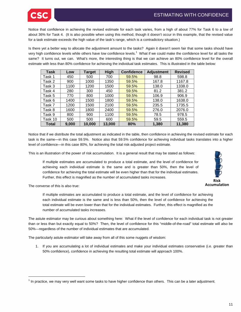
This is an illustration of the power of risk accumulation. It is a general result that may be stated as follows:

If multiple estimates are accumulated to produce a total estimate, and the level of confidence for achieving each individual estimate is the same and is greater than 50%, then the level of confidence for achieving the total estimate will be even higher than that for the individual estimates. Further, this effect is magnified as the number of accumulated tasks increases.

The converse of this is also true:

If multiple estimates are accumulated to produce a total estimate, and the level of confidence for achieving each individual estimate is the same and is less than 50%, then the level of confidence for achieving the total estimate will be even lower than that for the individual estimates. Further, this effect is magnified as the number of accumulated tasks increases.

The astute estimator may be curious about something here: What if the level of confidence for each individual task is not greater than or less than but exactly equal to 50%? Then, the level of confidence for this “middle-of-the-road” total estimate will also be 50%—regardless of the number of individual estimates that are accumulated.

The particularly astute estimator will take away from all of this some nuggets of wisdom:

1. If you are accumulating a lot of individual estimates and make your individual estimates conservative (i.e. greater than 50% confidence), confidence in achieving the resulting total estimate will approach 100%.

1 In practice, we may very well want some tasks to have higher confidence than others. This can be a later adjustment.

RiskAccumulation

12


2. If you are accumulating a lot of individual estimates and make your individual estimates aggressive (i.e. less than 50% confidence), confidence in achieving the resulting total estimate will approach 0%.

3. Estimate components conservatively!

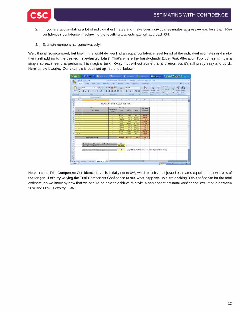
Well, this all sounds good, but how in the world do you find an equal confidence level for all of the individual estimates and make them still add up to the desired risk-adjusted total? That’s where the handy-dandy Excel Risk Allocation Tool comes in. It is a simple spreadsheet that performs this magical task. Okay, not without some trial and error, but it’s still pretty easy and quick. Here is how it works. Our example is seen set up in the tool below:

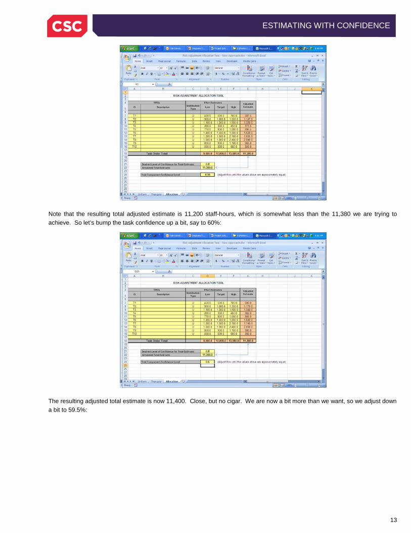
Note that the Trial Component Confidence Level is initially set to 0%, which results in adjusted estimates equal to the low levels of the ranges. Let’s try varying the Trial Component Confidence to see what happens. We are seeking 80% confidence for the total estimate, so we know by now that we should be able to achieve this with a component estimate confidence level that is between 50% and 80%. Let’s try 55%:

13


Note that the resulting total adjusted estimate is 11,200 staff-hours, which is somewhat less than the 11,380 we are trying to achieve. So let’s bump the task confidence up a bit, say to 60%:

The resulting adjusted total estimate is now 11,400. Close, but no cigar. We are now a bit more than we want, so we adjust down a bit to 59.5%:

14


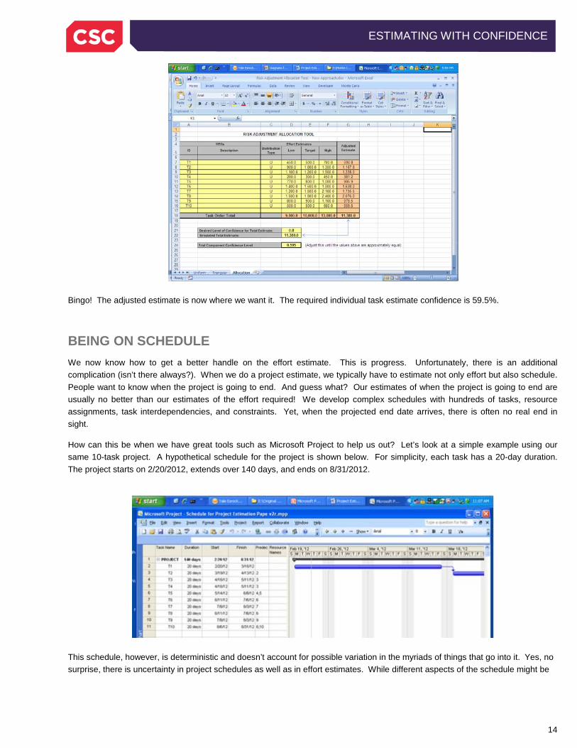
Bingo! The adjusted estimate is now where we want it. The required individual task estimate confidence is 59.5%.

BEING ON SCHEDULE We now know how to get a better handle on the effort estimate. This is progress. Unfortunately, there is an additional complication (isn’t there always?). When we do a project estimate, we typically have to estimate not only effort but also schedule. People want to know when the project is going to end. And guess what? Our estimates of when the project is going to end are usually no better than our estimates of the effort required! We develop complex schedules with hundreds of tasks, resource assignments, task interdependencies, and constraints. Yet, when the projected end date arrives, there is often no real end in sight.

How can this be when we have great tools such as Microsoft Project to help us out? Let’s look at a simple example using our same 10-task project. A hypothetical schedule for the project is shown below. For simplicity, each task has a 20-day duration. The project starts on 2/20/2012, extends over 140 days, and ends on 8/31/2012.

This schedule, however, is deterministic and doesn’t account for possible variation in the myriads of things that go into it. Yes, no surprise, there is uncertainty in project schedules as well as in effort estimates. While different aspects of the schedule might be

15


uncertain (for example, project start date, available resources, etc.) we will concentrate here on the most common source of variability: task durations.

Fortunately, we can use the same types of techniques, including Monte Carlo simulation, to address schedule variability. In this case, we use fuzzy numbers for uncertain task durations. Then the simulation results will tell us the probability of finishing the project by our desired completion date as well as the completion dates for any desired level of confidence.

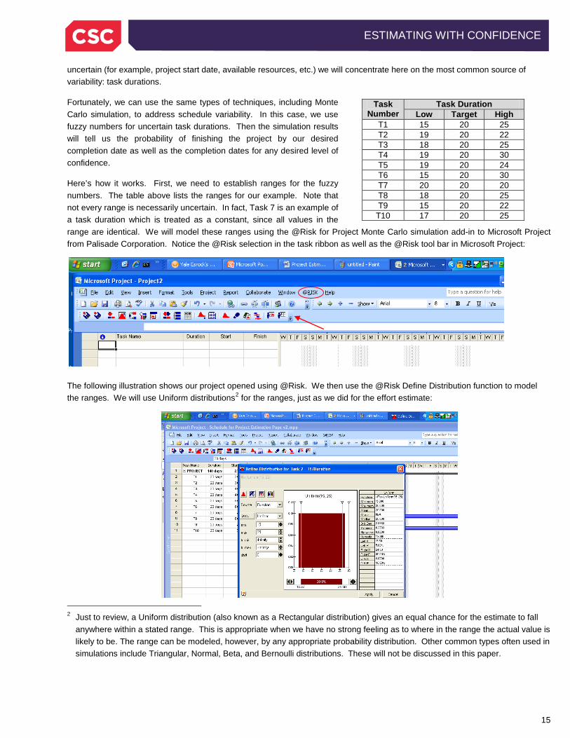
Here’s how it works. First, we need to establish ranges for the fuzzy numbers. The table above lists the ranges for our example. Note that not every range is necessarily uncertain. In fact, Task 7 is an example of a task duration which is treated as a constant, since all values in the range are identical. We will model these ranges using the @Risk for Project Monte Carlo simulation add-in to Microsoft Project from Palisade Corporation. Notice the @Risk selection in the task ribbon as well as the @Risk tool bar in Microsoft Project:

The following illustration shows our project opened using @Risk. We then use the @Risk Define Distribution function to model the ranges. We will use Uniform distributions2

for the ranges, just as we did for the effort estimate:

2 Just to review, a Uniform distribution (also known as a Rectangular distribution) gives an equal chance for the estimate to fall

anywhere within a stated range. This is appropriate when we have no strong feeling as to where in the range the actual value is likely to be. The range can be modeled, however, by any appropriate probability distribution. Other common types often used in simulations include Triangular, Normal, Beta, and Bernoulli distributions. These will not be discussed in this paper.

Task Number

Task Duration Low Target High

T1 15 20 25 T2 19 20 22 T3 18 20 25 T4 19 20 30 T5 19 20 24 T6 15 20 30 T7 20 20 20 T8 18 20 25 T9 15 20 22

T10 17 20 25

16


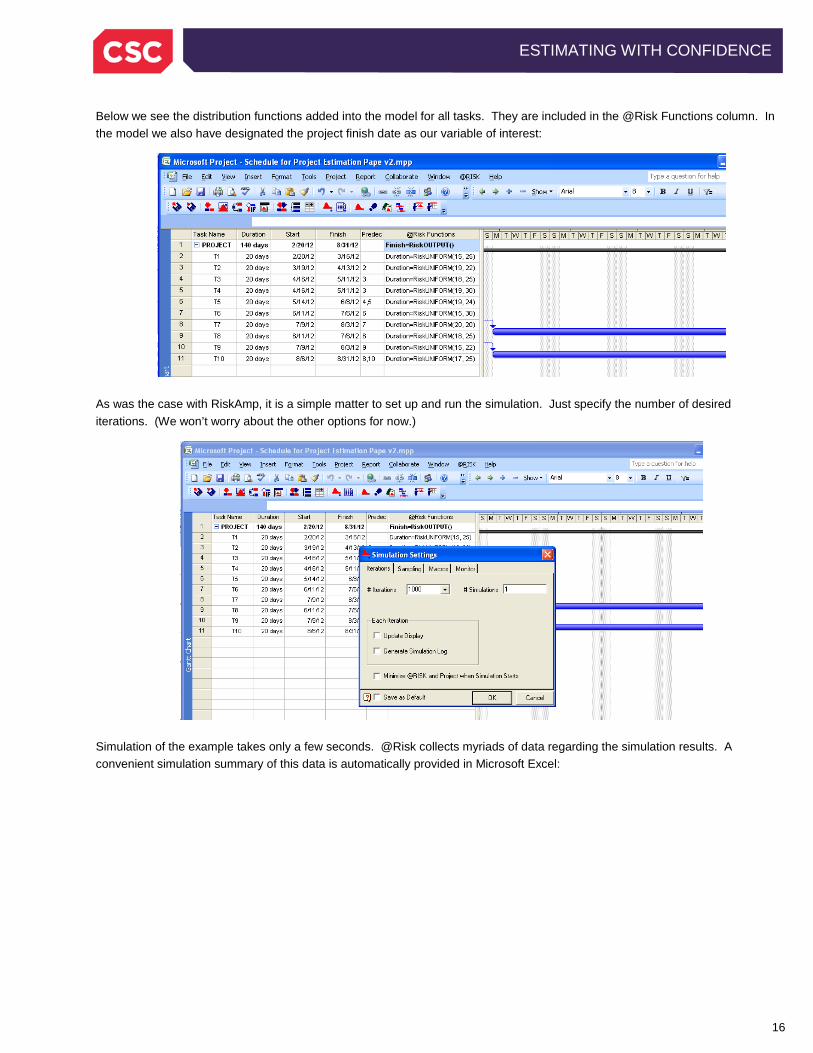
Below we see the distribution functions added into the model for all tasks. They are included in the @Risk Functions column. In the model we also have designated the project finish date as our variable of interest:

As was the case with RiskAmp, it is a simple matter to set up and run the simulation. Just specify the number of desired iterations. (We won’t worry about the other options for now.)

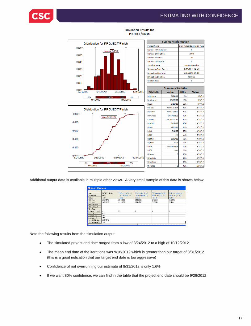
Simulation of the example takes only a few seconds. @Risk collects myriads of data regarding the simulation results. A convenient simulation summary of this data is automatically provided in Microsoft Excel:

17


Additional output data is available in multiple other views. A very small sample of this data is shown below:

Note the following results from the simulation output:

• The simulated project end date ranged from a low of 8/24/2012 to a high of 10/12/2012

• The mean end date of the iterations was 9/18/2012 which is greater than our target of 8/31/2012 (this is a good indication that our target end date is too aggressive)

• Confidence of not overrunning our estimate of 8/31/2012 is only 1.6%

• If we want 80% confidence, we can find in the table that the project end date should be 9/26/2012

18


There is an added bonus provided by the schedule simulation process, and it has to do with the project’s critical path. This falls into the category of “things we thought we knew”. Most Schedulers and Project Managers are well-acquainted with the venerable concept of critical path. It’s pretty straightforward—the critical path is the longest path through a network of tasks, and any delay on any task that is part of the critical path will delay the project by the same amount.

Well, there is a slight problem created when we start using fuzzy numbers for task durations: the critical path may end up not being the critical path! Once duration variability is recognized, we can no longer definitively say that a task is on the critical path. There is only a tendency to be on the critical path. This tendency is measured by something called the critical index. This is a value between 0 and 1 that measures the likelihood that a task will be on the critical path. A critical index of 0 means the task is never on the critical path, a value of 1 means it is always on the critical path, a value of .5 means there is a 50% probability that it is on the critical path. You get the picture.

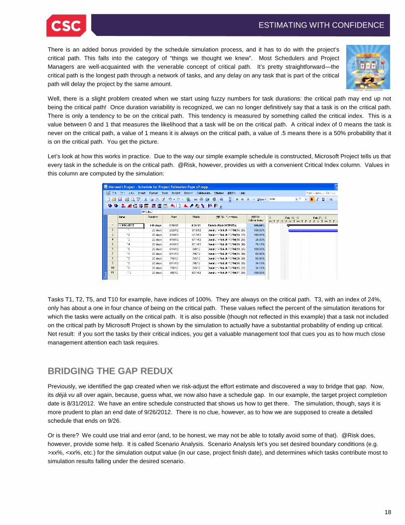
Let’s look at how this works in practice. Due to the way our simple example schedule is constructed, Microsoft Project tells us that every task in the schedule is on the critical path. @Risk, however, provides us with a convenient Critical Index column. Values in this column are computed by the simulation:

Tasks T1, T2, T5, and T10 for example, have indices of 100%. They are always on the critical path. T3, with an index of 24%, only has about a one in four chance of being on the critical path. These values reflect the percent of the simulation iterations for which the tasks were actually on the critical path. It is also possible (though not reflected in this example) that a task not included on the critical path by Microsoft Project is shown by the simulation to actually have a substantial probability of ending up critical. Net result: if you sort the tasks by their critical indices, you get a valuable management tool that cues you as to how much close management attention each task requires.

BRIDGING THE GAP REDUX Previously, we identified the gap created when we risk-adjust the effort estimate and discovered a way to bridge that gap. Now, its déjà vu all over again, because, guess what, we now also have a schedule gap. In our example, the target project completion date is 8/31/2012. We have an entire schedule constructed that shows us how to get there. The simulation, though, says it is more prudent to plan an end date of 9/26/2012. There is no clue, however, as to how we are supposed to create a detailed schedule that ends on 9/26.

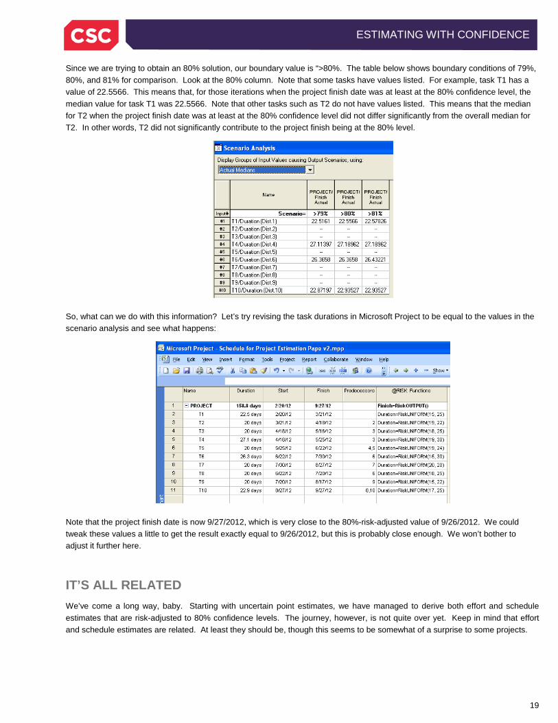
Or is there? We could use trial and error (and, to be honest, we may not be able to totally avoid some of that). @Risk does, however, provide some help. It is called Scenario Analysis. Scenario Analysis let’s you set desired boundary conditions (e.g. >xx%, <xx%, etc.) for the simulation output value (in our case, project finish date), and determines which tasks contribute most to simulation results falling under the desired scenario.

19


Since we are trying to obtain an 80% solution, our boundary value is “>80%. The table below shows boundary conditions of 79%, 80%, and 81% for comparison. Look at the 80% column. Note that some tasks have values listed. For example, task T1 has a value of 22.5566. This means that, for those iterations when the project finish date was at least at the 80% confidence level, the median value for task T1 was 22.5566. Note that other tasks such as T2 do not have values listed. This means that the median for T2 when the project finish date was at least at the 80% confidence level did not differ significantly from the overall median for T2. In other words, T2 did not significantly contribute to the project finish being at the 80% level.

So, what can we do with this information? Let’s try revising the task durations in Microsoft Project to be equal to the values in the scenario analysis and see what happens:

Note that the project finish date is now 9/27/2012, which is very close to the 80%-risk-adjusted value of 9/26/2012. We could tweak these values a little to get the result exactly equal to 9/26/2012, but this is probably close enough. We won’t bother to adjust it further here.

IT’S ALL RELATED We’ve come a long way, baby. Starting with uncertain point estimates, we have managed to derive both effort and schedule estimates that are risk-adjusted to 80% confidence levels. The journey, however, is not quite over yet. Keep in mind that effort and schedule estimates are related. At least they should be, though this seems to be somewhat of a surprise to some projects.

20


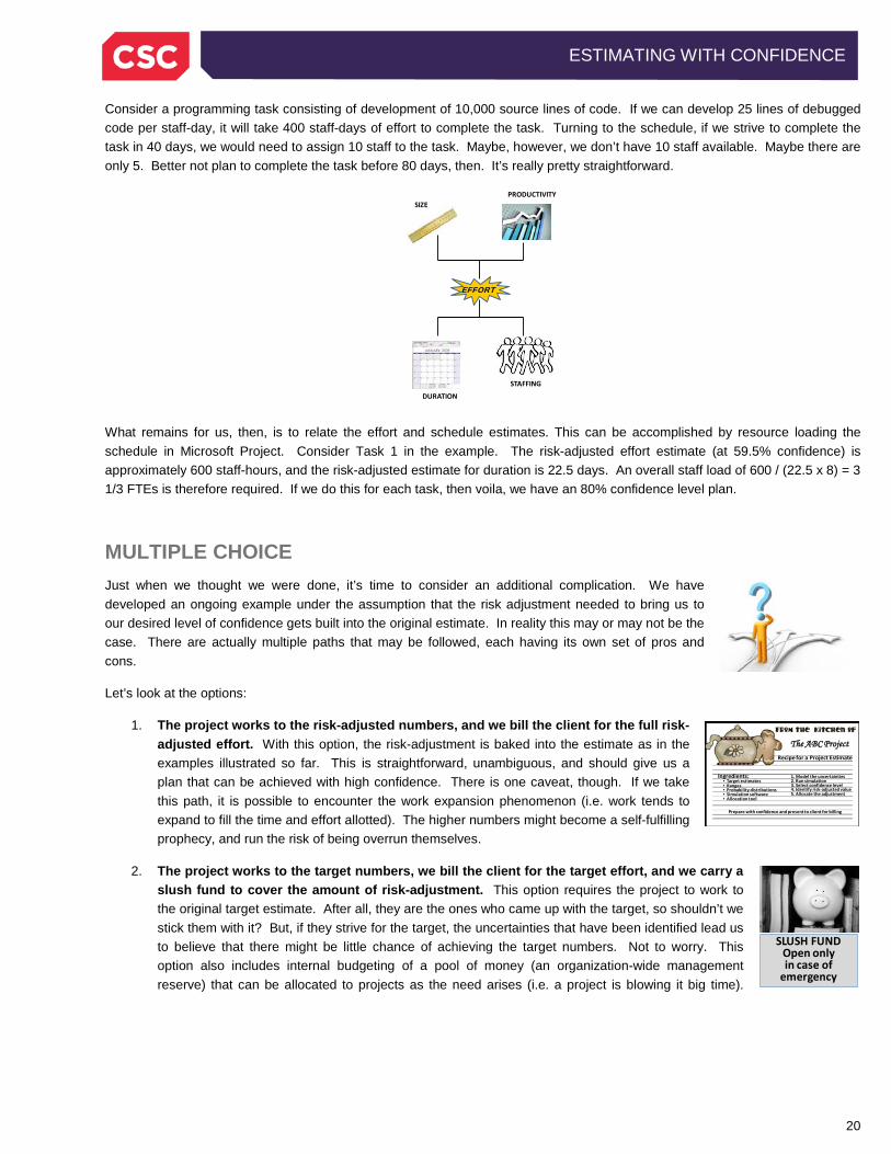
Consider a programming task consisting of development of 10,000 source lines of code. If we can develop 25 lines of debugged code per staff-day, it will take 400 staff-days of effort to complete the task. Turning to the schedule, if we strive to complete the task in 40 days, we would need to assign 10 staff to the task. Maybe, however, we don’t have 10 staff available. Maybe there are only 5. Better not plan to complete the task before 80 days, then. It’s really pretty straightforward.

What remains for us, then, is to relate the effort and schedule estimates. This can be accomplished by resource loading the schedule in Microsoft Project. Consider Task 1 in the example. The risk-adjusted effort estimate (at 59.5% confidence) is approximately 600 staff-hours, and the risk-adjusted estimate for duration is 22.5 days. An overall staff load of 600 / (22.5 x 8) = 3 1/3 FTEs is therefore required. If we do this for each task, then voila, we have an 80% confidence level plan.

MULTIPLE CHOICE Just when we thought we were done, it’s time to consider an additional complication. We have developed an ongoing example under the assumption that the risk adjustment needed to bring us to our desired level of confidence gets built into the original estimate. In reality this may or may not be the case. There are actually multiple paths that may be followed, each having its own set of pros and cons.

Let’s look at the options:

1. The project works to the risk-adjusted numbers, and we bill the client for the full risk-adjusted effort. With this option, the risk-adjustment is baked into the estimate as in the examples illustrated so far. This is straightforward, unambiguous, and should give us a plan that can be achieved with high confidence. There is one caveat, though. If we take this path, it is possible to encounter the work expansion phenomenon (i.e. work tends to expand to fill the time and effort allotted). The higher numbers might become a self-fulfilling prophecy, and run the risk of being overrun themselves.

2. The project works to the target numbers, we bill the client for the target effort, and we carry a slush fund to cover the amount of risk-adjustment. This option requires the project to work to the original target estimate. After all, they are the ones who came up with the target, so shouldn’t we stick them with it? But, if they strive for the target, the uncertainties that have been identified lead us to believe that there might be little chance of achieving the target numbers. Not to worry. This option also includes internal budgeting of a pool of money (an organization-wide management reserve) that can be allocated to projects as the need arises (i.e. a project is blowing it big time).

EFFORT

SIZEPRODUCTIVITY

DURATION

STAFFING

The ABC ProjectRecipe for a Project Estimate

Ingredients:• Target estimates• Ranges• Probability distributions• Simulation software• Allocation tool

1. Model the uncertainties2. Run simulation3. Select confidence level4. Identify risk-adjusted value5. Allocate the adjustment

Prepare with confidence and present to client for billing

SLUSH FUNDOpen onlyin case of

emergency

21


The amount of a project’s risk-adjustment would be reserved against the overall pool so the project will have funds, if needed. The client, of course, is only billed for the target effort since we are covering the cost of the risk-adjustment internally. Okay, maybe this isn’t a likely scenario, but it’s an option.

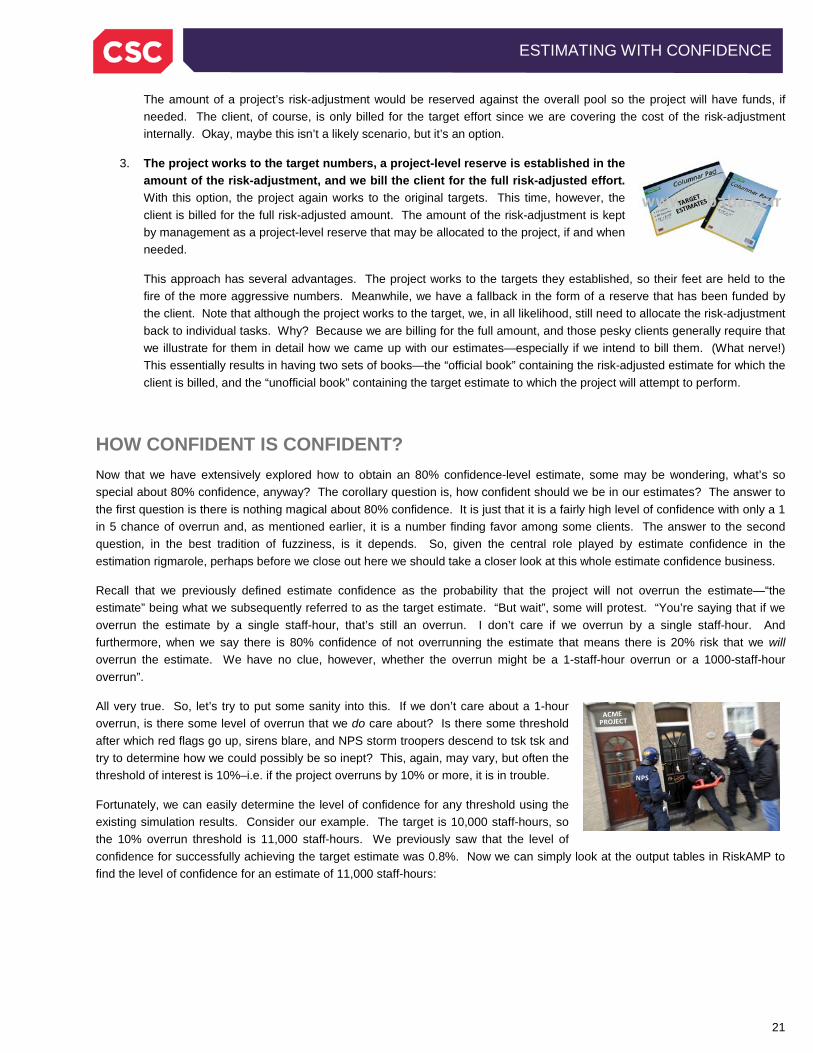
3. The project works to the target numbers, a project-level reserve is established in the amount of the risk-adjustment, and we bill the client for the full risk-adjusted effort. With this option, the project again works to the original targets. This time, however, the client is billed for the full risk-adjusted amount. The amount of the risk-adjustment is kept by management as a project-level reserve that may be allocated to the project, if and when needed.

This approach has several advantages. The project works to the targets they established, so their feet are held to the fire of the more aggressive numbers. Meanwhile, we have a fallback in the form of a reserve that has been funded by the client. Note that although the project works to the target, we, in all likelihood, still need to allocate the risk-adjustment back to individual tasks. Why? Because we are billing for the full amount, and those pesky clients generally require that we illustrate for them in detail how we came up with our estimates—especially if we intend to bill them. (What nerve!) This essentially results in having two sets of books—the “official book” containing the risk-adjusted estimate for which the client is billed, and the “unofficial book” containing the target estimate to which the project will attempt to perform.

HOW CONFIDENT IS CONFIDENT? Now that we have extensively explored how to obtain an 80% confidence-level estimate, some may be wondering, what’s so special about 80% confidence, anyway? The corollary question is, how confident should we be in our estimates? The answer to the first question is there is nothing magical about 80% confidence. It is just that it is a fairly high level of confidence with only a 1 in 5 chance of overrun and, as mentioned earlier, it is a number finding favor among some clients. The answer to the second question, in the best tradition of fuzziness, is it depends. So, given the central role played by estimate confidence in the estimation rigmarole, perhaps before we close out here we should take a closer look at this whole estimate confidence business.

Recall that we previously defined estimate confidence as the probability that the project will not overrun the estimate—“the estimate” being what we subsequently referred to as the target estimate. “But wait”, some will protest. “You’re saying that if we overrun the estimate by a single staff-hour, that’s still an overrun. I don’t care if we overrun by a single staff-hour. And furthermore, when we say there is 80% confidence of not overrunning the estimate that means there is 20% risk that we will overrun the estimate. We have no clue, however, whether the overrun might be a 1-staff-hour overrun or a 1000-staff-hour overrun”.

All very true. So, let’s try to put some sanity into this. If we don’t care about a 1-hour overrun, is there some level of overrun that we do care about? Is there some threshold after which red flags go up, sirens blare, and NPS storm troopers descend to tsk tsk and try to determine how we could possibly be so inept? This, again, may vary, but often the threshold of interest is 10%–i.e. if the project overruns by 10% or more, it is in trouble.

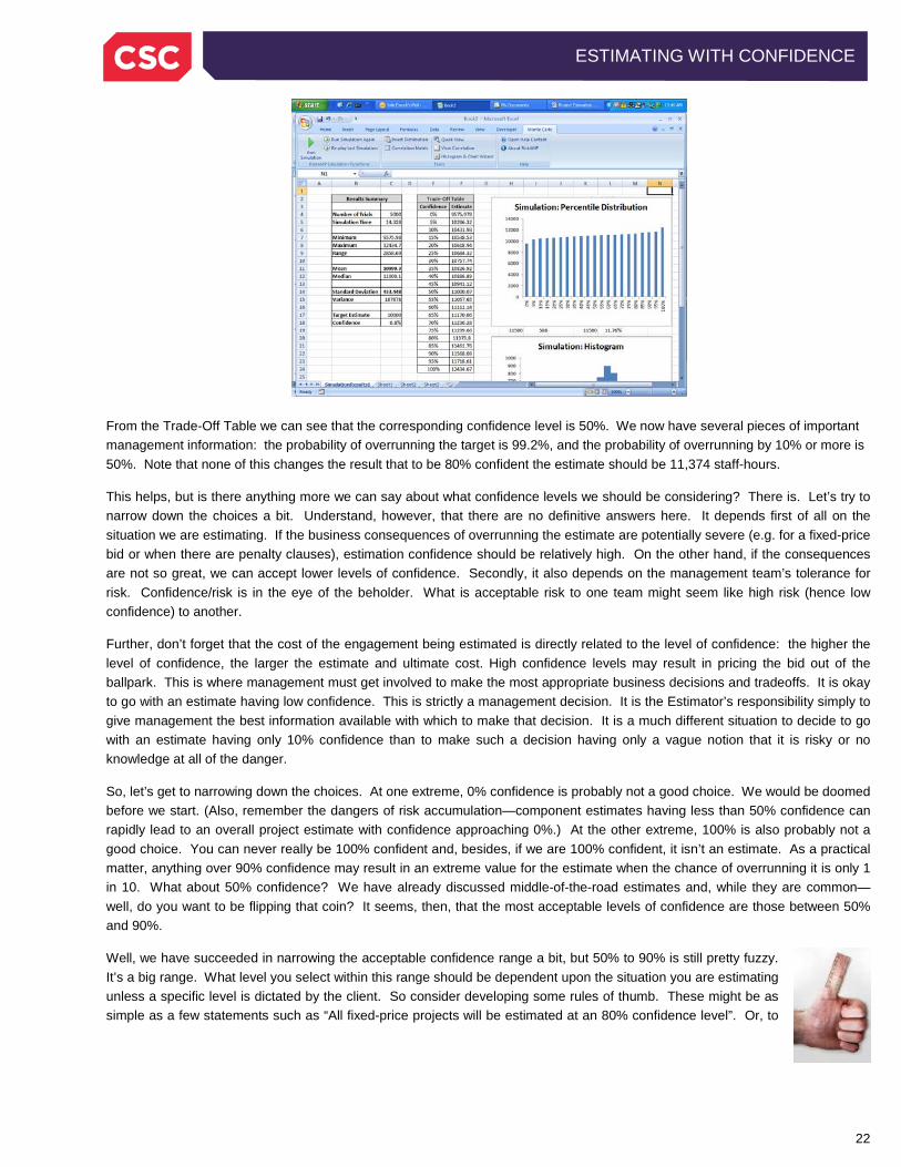
Fortunately, we can easily determine the level of confidence for any threshold using the existing simulation results. Consider our example. The target is 10,000 staff-hours, so the 10% overrun threshold is 11,000 staff-hours. We previously saw that the level of confidence for successfully achieving the target estimate was 0.8%. Now we can simply look at the output tables in RiskAMP to find the level of confidence for an estimate of 11,000 staff-hours:

NPS

22


From the Trade-Off Table we can see that the corresponding confidence level is 50%. We now have several pieces of important management information: the probability of overrunning the target is 99.2%, and the probability of overrunning by 10% or more is 50%. Note that none of this changes the result that to be 80% confident the estimate should be 11,374 staff-hours.

This helps, but is there anything more we can say about what confidence levels we should be considering? There is. Let’s try to narrow down the choices a bit. Understand, however, that there are no definitive answers here. It depends first of all on the situation we are estimating. If the business consequences of overrunning the estimate are potentially severe (e.g. for a fixed-price bid or when there are penalty clauses), estimation confidence should be relatively high. On the other hand, if the consequences are not so great, we can accept lower levels of confidence. Secondly, it also depends on the management team’s tolerance for risk. Confidence/risk is in the eye of the beholder. What is acceptable risk to one team might seem like high risk (hence low confidence) to another.

Further, don’t forget that the cost of the engagement being estimated is directly related to the level of confidence: the higher the level of confidence, the larger the estimate and ultimate cost. High confidence levels may result in pricing the bid out of the ballpark. This is where management must get involved to make the most appropriate business decisions and tradeoffs. It is okay to go with an estimate having low confidence. This is strictly a management decision. It is the Estimator’s responsibility simply to give management the best information available with which to make that decision. It is a much different situation to decide to go with an estimate having only 10% confidence than to make such a decision having only a vague notion that it is risky or no knowledge at all of the danger.

So, let’s get to narrowing down the choices. At one extreme, 0% confidence is probably not a good choice. We would be doomed before we start. (Also, remember the dangers of risk accumulation—component estimates having less than 50% confidence can rapidly lead to an overall project estimate with confidence approaching 0%.) At the other extreme, 100% is also probably not a good choice. You can never really be 100% confident and, besides, if we are 100% confident, it isn’t an estimate. As a practical matter, anything over 90% confidence may result in an extreme value for the estimate when the chance of overrunning it is only 1 in 10. What about 50% confidence? We have already discussed middle-of-the-road estimates and, while they are common—well, do you want to be flipping that coin? It seems, then, that the most acceptable levels of confidence are those between 50% and 90%.

Well, we have succeeded in narrowing the acceptable confidence range a bit, but 50% to 90% is still pretty fuzzy. It’s a big range. What level you select within this range should be dependent upon the situation you are estimating unless a specific level is dictated by the client. So consider developing some rules of thumb. These might be as simple as a few statements such as “All fixed-price projects will be estimated at an 80% confidence level”. Or, to

23


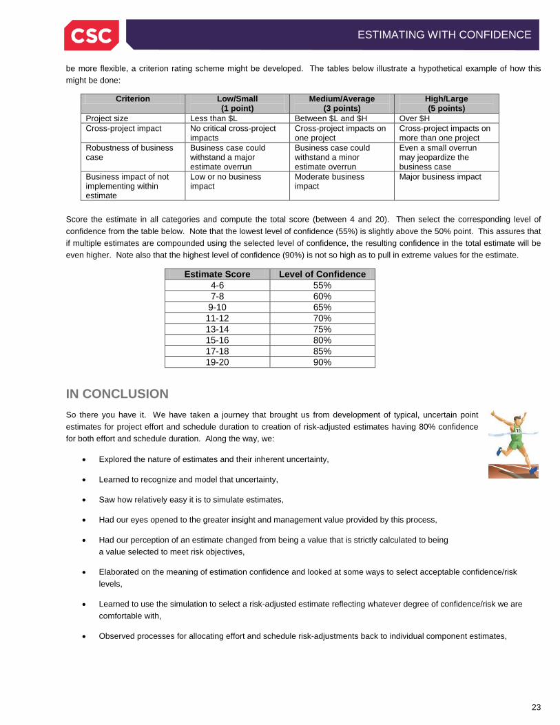
be more flexible, a criterion rating scheme might be developed. The tables below illustrate a hypothetical example of how this might be done:

Criterion Low/Small (1 point)

Medium/Average (3 points)

High/Large (5 points)

Project size Less than $L Between $L and $H Over $H Cross-project impact No critical cross-project

impacts Cross-project impacts on one project

Cross-project impacts on more than one project

Robustness of business case

Business case could withstand a major estimate overrun

Business case could withstand a minor estimate overrun

Even a small overrun may jeopardize the business case

Business impact of not implementing within estimate

Low or no business impact

Moderate business impact

Major business impact

Score the estimate in all categories and compute the total score (between 4 and 20). Then select the corresponding level of confidence from the table below. Note that the lowest level of confidence (55%) is slightly above the 50% point. This assures that if multiple estimates are compounded using the selected level of confidence, the resulting confidence in the total estimate will be even higher. Note also that the highest level of confidence (90%) is not so high as to pull in extreme values for the estimate.

Estimate Score Level of Confidence 4-6 55% 7-8 60%

9-10 65% 11-12 70% 13-14 75% 15-16 80% 17-18 85% 19-20 90%

IN CONCLUSION So there you have it. We have taken a journey that brought us from development of typical, uncertain point estimates for project effort and schedule duration to creation of risk-adjusted estimates having 80% confidence for both effort and schedule duration. Along the way, we:

• Explored the nature of estimates and their inherent uncertainty,

• Learned to recognize and model that uncertainty,

• Saw how relatively easy it is to simulate estimates,

• Had our eyes opened to the greater insight and management value provided by this process,

• Had our perception of an estimate changed from being a value that is strictly calculated to being a value selected to meet risk objectives,

• Elaborated on the meaning of estimation confidence and looked at some ways to select acceptable confidence/risk levels,

• Learned to use the simulation to select a risk-adjusted estimate reflecting whatever degree of confidence/risk we are comfortable with,

• Observed processes for allocating effort and schedule risk-adjustments back to individual component estimates,

24


• Derived a cohesive set of effort and schedule estimates that are each internally consistent, consistent with each other, and both risk-adjusted to 80% confidence levels,

• Explored multiple options for accounting for the risk-adjustment, including the role of management reserve, and

• Witnessed the use of actual software tools for accomplishing all of this.

A word of caution in closing: The techniques presented in this paper are valid for use in all types of estimation from detailed to very rough order of magnitude (VROM) estimates. Results, however, are strictly dependent on the estimator’s ability and willingness to identify estimation ranges that portray the true span of potential outcomes.

DISCLAIMER The information, views and opinions expressed in this paper constitute solely the authors’ views and opinions and do not represent in any way CSC’s official corporate views and opinions. The authors have made every attempt to ensure that the information contained in this paper has been obtained from reliable sources. CSC is not responsible for any errors or omissions or for the results obtained from the use of this information. All information in this paper is provided “as is,” with no guarantee by CSC of completeness, accuracy, timeliness or the results obtained from the use of this information, and without warranty of any kind, express or implied, including but not limited to warranties of performance, merchantability and fitness for a particular purpose. In no event will CSC, its related partnerships or corporations, or the partners, agents or employees thereof be liable to you or anyone else for any decision made or action taken in reliance on the information in this paper or for any consequential, special or similar damages, even if advised of the possibility of such damages.

Copyright © 2013 Computer Sciences Corporation. All rights reserved.

EstimatorsTake Heed

Documents

ESTIMATING WITH CONFIDENCE - DXC Technologyassets1.csc.com/innovation/downloads/Estimating_with_Confidence.… · 2 ESTIMATING WITH CONF IDENCE chicken and egg thing. Let’s ignore