Final report

Estimating value added in Rwanda’s domestic trade

Ewoud Nijhof Victor Steenbergen John Spray November 2018 When citing this paper, please use the title and the followingreference number:F-38409-RWA-1

Estimating Value Added in Rwanda’s Domestic Trade Ewoud Nijhof, Victor Steenbergen and John Spray

In Brief

This paper introduces a new economic dataset for Rwanda, which provides unique insights intoeach formal firm’s input sourcing, production, and productivity by product. This paper firstexplains the underlying technology which made this possible: Electronic Billing Machines (EBMs). Next, we provide details on how we processed EBM data into a dataset suitable for economic analysis using machine learning for product classification and to identify each firm’s value-add per product. The paper then provides key summary statistics of the dataset and conducts sensitivity analysis by comparing it to other measures of Rwanda’s output (e.g. Rwanda’s macro-accounts).Finally, we offer a number of potential future applications of this new value-added dataset forRwanda. We conclude there is still work to be done to improve the accessibility of the EBM data further, but that the potential of the EBM data is worth exploring.

1. IntroductionOver the past decades, Rwanda has been working hard to develop the economy. The past few years, the government has been devoted to promoting domestic production and trade through theMade in Rwanda (MiR) policy (MINEACOM, 2017). One of the more specific targets of this policy is to improve so-called backward linkages of multinational companies (MNC) which have a presence in Rwanda. Backward linkages are the local supply ties a MNC uses. More and stronger backward linkages providing a boost to local firms means the Rwandan economy as a whole benefits more from the presence of the MNC.

To improve these linkages, it is vital to identify successful companies and partnerships on the one hand and constraints for MNCs to use local suppliers on the other. Unfortunately for most countries, there is very little product level data on trade between companies. This means most countries have a hard time identifying successful products being produced and trade domestically. Rwanda however, has been working hard to roll out Electronic Billing Machines (EBM) which produce official receipts for each formal sale. The Rwandan Revenue Authority (RRA) has access to this information for all VAT-registered firms.

This paper introduces a new economic dataset for Rwanda, which provides unique insights intoeach formal firm’s input sourcing, production, and productivity by product. This paper firstexplains the underlying data which makes this possible: Electronic Billing Machines (EBMs). Next,we note the extensive data processing to make EBMs suitable for economic analysis, whichincludes using machine learning to classify products and identify each firm’s value-added perproduct. We show that we are able to process the data into a dataset that is very useful for economic analysis. The paper then provides key summary statistics of the dataset and conducts sensitivity analysis by comparing it to other measures of Rwanda’s output (e.g. Rwanda’s macro-accounts). Finally, we offer a number of potential future applications of this new value-added dataset for Rwanda.

We start in chapter 2 by identifying the source of the data and current problems of accessing it. Chapter 3 then describes the data in more detail. In chapter 4, we delve into how we processed the EBM data to make it more useful for economic analysis. We show descriptive statistics of the output along with robustness checks in chapter 5. Finally, in chapter 6, we layout further work that needs to be done to be able to fully utilize the data. In that chapter, we also provide insight into different potential applications of the data. IGC has already used the database to identify the potential for backward linkages, in the IGC working paper “Potential for Backward Linkages” (Spray and Steenbergen, 2018). This preliminary use of the database speaks to its potential.

2. Data Source and Identifying Data Challenges

Data source: Electronic Billing MachinesThe main data source relevant for this paper is data collected from Electronic Billing Machines (EBM). This section provides more detail on what exactly an EBM is, how it is used, as well as the current challenges are in accessing this data.

In Rwanda, all companies registered for Value Added Tax (VAT), meaning all companies exceeding RWF 20 million in yearly turnover, are legally obligated to have an Electronic Billing Machine (EBM)1. The EBM could help in the filing of their VAT. Eissa et al. (2014) show that indeed VAT compliance has grown since the introduction of EBMs, though Steenbergen (2017) shows that there is still room for improvement. The EBMs record every sale and produce official receipts for customers. Often, cashiers manually input data into the EBM. The sales data for each VAT registered company in Rwanda is then uploaded onto the RRA’s database. The level of detail and extensive coverage comprehensiveness is where the data mainly differs from more common VAT oreven VAT annex data. Earlier studies show that EBM is more widespread for medium and bigger firms (Eissa et al., 2014). EBM receipts are also more often issued for expensive items, and on average EBM receipts are issued to consumers only about 5-9% of the time for transactions under 10.000RWF (IGC,2017). This is despite 78% of taxpaying firms having an EBM as of 2014, a numberthat is very likely to have grown significantly since.

Data format: EBM receiptsThe receipts issued by the EBMs have a standard format and contain standardized information: theTax Identification Number (TIN) of the seller, number of items sold and total worth, applicable VAT rate, total of the receipt and an item label, which is sometimes automatically scanned but most often manually entered by the cashier. The EBMs also assign a unique signature to the receipt. Optionally, the TIN of the customer is registered if provided. For business to business sales, the TINof the buying firm is required to claim back VAT paid to suppliers, meaning all VAT registered business will record their TIN when buying. Few consumers will register their TIN, unless they are eligible for some sort of VAT exemption.

Laterite2 has compiled a detailed description of the receipts format, shown in figure 1 (Laterite, 2018). It divides the receipt into two main categories: the item description and the other sections. The latter contains relatively standardized information, accessible in XML format by the RRA, and mostly contain information required by law. The item description however contains unit quantity and total worth, but the actual description is up to the cashier, resulting in widely varying item descriptions. An item line is comprised of the item description, the quantity of that item, and the total worth for that quantity.

1 According to VAT law N° 37/2012 of 09/11/2012, article 24.2 Laterite is a data, research and technical advisory firm that works to understand and analyse complex development challenges.

Figure 1: Example and different sections of an EBM Receipt, compiled by Laterite.1 ABC BUSINESS

KIMIRONKO-GASABO-KIGALI TEL:0781234567 TIN: 123456789 ------------------------

Receipt header (designator information)This section is usually relatively short and contains mandatory business identification information (business name and TIN). It often contains the business address and telephone number, and occasionally other information such as client name and TIN.

2 6 * 950.00 IBASI 5700.00 B------------------------

Item descriptionThis section varies in length from one line to hundreds of lines. The layouts also vary greatly but most receipts use a small subset of layouts.

3 TOTAL 5700.00 TOTAL B-18.00% 5700.00TOTAL TAX B 869.49TOTAL TAX 869.49------------------------CASH 5700.00items number 01------------------------

Tax informationThis section has a reasonably consistent layout and always contains core mandatory information summarizing the transaction and the tax liability. It occasionally contains some additional information (e.g. paid and change).

4 SDC Information D/T: 02/11/2016 11:27:09SDC ID: SDC002000534 RECEIPT NUMBER: 35090/40431 NSInternal Data: LUUC-D5RR-BXI2-2OBB 4E34-DUHN-CQ Receipt Signature: VRQG-B7Q3-BFX4-2SZS ------------------------RECEIPT NUMBER: 8771D/T: 02/11/2016 11:26:17MRC: INZ01001247 ------------------------ END ........................

SDC informationThis section has the most consistent layout and all receipts contains the same mandatory SDC information. At the bottom of the receipt, there is often generic footer text (e.g. End; Thank you for your business) and occasionally receipt specific information (e.g. client TIN).

Data descriptionEBM data has varying degrees of completeness and consistency. For example, the TIN of the buyer is sometimes recorded, generally when the buyer is a business. Quantity is often just entered as 1, even though the total cost suggests higher quantities. Item descriptions are often missing or not legible, such as Dept.01 for all products. Table 1 shows a complete list of variables that appear in the raw receipt data, where the starred variables are used in the final analysis. Some, for example the SDC receipt signature, were used in the intermediate processing, for example to identify

individual receipts.

Table 1: description of relevant variables in the dataset. The starred variables appear in the final database.Variable name Variable description

TIN Tax Identification Number of the selling firm, which uniquely identifies the firm and is assigned by the RRA. To anonymize the data we converted the TIN into a random ID number, only accessible to the original researcher.

ClientsTIN TIN of the buying firm or person, if provided. We used the same anonymizationfor the sellers, so we can match bought and sold products to the same ID.

id_supplier * Randomly assigned number for the seller to replace the TIN, to anonymize the data.

id_client* Randomly assigned number for the buyer to replace the clients TIN. Matches tothe id_supplier if the same firm both appears as buyer and seller.

Total* Worth of the item line in Rwandan Francs (RWF), the item line containing just one type of item, with varying quantities per item. The price per item could notbe extracted consistently.

Unit_quantity* Number of items sold per item type. Not always present.

Size Size of the item being sold as extracted from the item description. Unfortunately not consistently available and extractable.

Item Original text input as extracted from the receipt.

Spell_checked Checked and adjusted text input to match French, Kinyarwanda or English words.

Translate Translated text input, translated from French and Kinyarwanda into English. Final input for the tagging process

Hs4-predictions* The Harmonized Systems 4-digit code for the item, as predicted by a machine learning algorithm.

SdcReceipt-Signature

Automatically assigned signature by the EBM, identifying a unique receipt. Used to extract items per receipt.

B2b* Identifying a business to business sale, based on whether there is an id_client present in the data.

B2c* Identifying a business to consumer sale, when the id_client was missing. Different consumers cannot be distinguished, so all consumers are seen as a single buyer.

Total_bought-hs4*

The amount (RWF) for which the selling firm has bought products with the same code.

Total_inputs * Total cost (RWF) of the selling firm of all products bought in the EBM data plus labour cost

profit_share* The profit margin of the selling firm, assumed to be constant per firm. The exact computation is shown in chapter 3.

Value_added* Profit_share x total, to show value added by the sale or product flow

Median_margin- The profit share calculated by product by International Standard Industrial

isic* Classification (ISIC) sector.sExact computation is shown in chapter 3.

new_value-added*

The value added computed using the median_margin_isic by multiplying median_margin_isic by total.

Mainentact* The main activity of the selling firm, as registered by the RRA. Generally the same or very similar to the ISIC code.

Isicdesc* The standardized description of the ISIC code Variable nameVariable de

In total, some 25 million receipts (equal to the number of transactions recorded) were used in the analysis. These were parsed into roughly 58 million item lines, with varying quantities per item line. Our data covers 11,243 different supplier firms and 56,207 client firms (excluding consumers), of which 44,602 show up exclusively as client firms without registered sales. See table 2 for more descriptive statistics.

Table 2: selected descriptive statistics of the input dataName Description Data

Number of firms total Total number of firms in EBM database 56,207

- of which solely buyers Number of firms with no sales, only bought products in database

44,602

- of which solely suppliers Number of firms with no bought products, only sales in database

362

- of which combined buyer and supplier

Number of firms with both bought products and sales in database

11,243

Number of transactions Number of recorded transactions, i.e. number of receipts

~ 25,000,000

Number of item lines Number of individually recorded items sold, with varying quantities

~ 60,000,000

Number of items sold Total quantity of items sold. Some items did not have the quantity listed

632,598,577

- of which to businesses Total quantity sold by a business to a business

305,656,829

- of which to consumers Total quantity sold by a business to a consumer

326,941,748

Sum of total sales Total worth(RWF) of all sales in the EBM data

5,229,320,235,765

- of which to businesses Total worth (RWF) of all EBM sales between two businesses

2,128,452,762,005

- of which to consumers Total worth (RWF) all EBM sales of a business to a consumer

3,100,867,473,760

Sum of inputs Total labour cost plus worth of products bought by a selling firm (RWF)

6,228,380,683,082

Challenges with EBM dataData with this level of detail is bound to come with its challenges. First and foremost on the completeness and reliability of data. As shown in Eissa et al. (2014) firms might: i) not use their EBM, ii) not use it inconsistently, iii) the EBM breaks, runs out of power or airtime. This is further illustrated by the fact that over 180 firms, 1.5% of total firms in the set, have a registered EBM sales value of less than 1000 RWF, a negligible amount. Even more intriguing is that almost half of the firms, just short of 5000 firms, have an EBM sales value of less than 20 million RWF, the minimum to register for VAT. In general, we can assume the data is quite complete for medium to large firms, since most of these firms have activated EBM machines and the RRA effectively enforces EBM laws. However, in the first version of EBM used by over 90% of firms, much of the data is entered manually, resulting in TINs and phone numbers used as quantities, prices or item names, entries being off by a factor 100 or 1000 (especially given the relatively limited worth of 1 RWF) and often missing or convenient numbers (1) for some variables. In summary, we can assume a fairly complete census of VAT-registered firms, but not for the firms around or under the threshold. We will also have to be aware that the EBM data will have large

caveats on the transaction level, and contains any number of data errors. As an illustration, there was a single sale with a value of over 20 billion USD, about 3 times the total Rwandan GDP.

A specific obstacle to make meaningful use of the item level data is the manually entered item names. Product names are entered in 3 to 4 languages, using both brand names and product names, different degrees of abbreviation, and often just convenient shorthand such as 'Dept 01' instead of names. Variation is huge between firms, but also within firms or even for the same employee the same product might go by different names, with coherent naming conventions seldom being identifiable. The resulting product level data, though very rich, is therefore extremelyhard to analyse without extensive manipulation and does not really add information over the receipt level data. The result is that the RRA itself uses mostly the more readily available receipt level data. A major contribution of the IGC is to attempt to assign product level codes to these items. Chapter 3 describes the machine learning algorithm used to tackle the naming problem and create a proper product level database.

Another challenge with the EBM data is the fact that it only shows gross sales data rather than value added. Gross sales data means that many economic activities are double-counted in the data, for example transactions for throughput sectors like transport and storage and relevant economic production is attributed to the wrong firms. The data only really shows another estimatefor turnover when just using gross sales, for which VAT data or even CIT would be easier, more reliable and more complete, meaning without further analysis the EBM data offers no additional benefits. We explain this further in chapter 4, where we elaborate on the calculation of value added and the difference between gross trade and trade in value added.

These two main challenges; the lack of standardization and the raw form of gross sales data, are the main reasons why the EBM data is currently underutilized. Solving for these challenges is the main goal of this paper. We describe our approach for solving the standardization problem in the next chapter.

3. The Input Data and Classifying Items

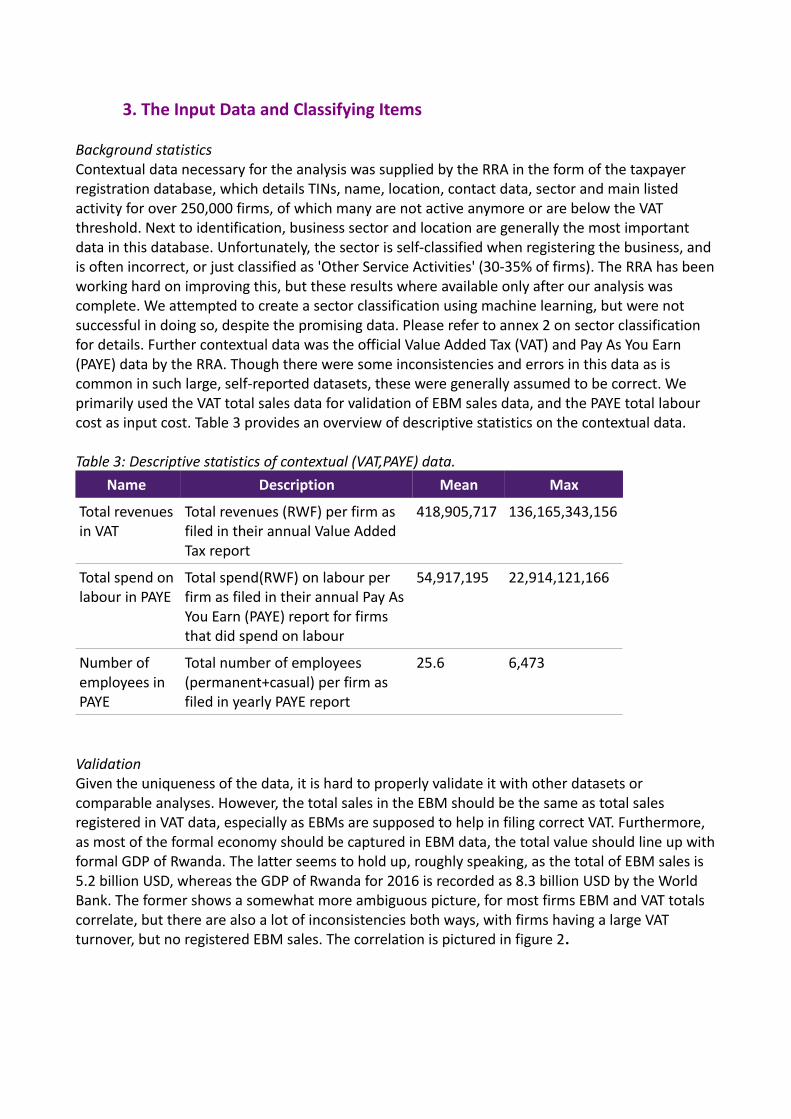
Background statisticsContextual data necessary for the analysis was supplied by the RRA in the form of the taxpayer registration database, which details TINs, name, location, contact data, sector and main listed activity for over 250,000 firms, of which many are not active anymore or are below the VAT threshold. Next to identification, business sector and location are generally the most important data in this database. Unfortunately, the sector is self-classified when registering the business, and is often incorrect, or just classified as 'Other Service Activities' (30-35% of firms). The RRA has beenworking hard on improving this, but these results where available only after our analysis was complete. We attempted to create a sector classification using machine learning, but were not successful in doing so, despite the promising data. Please refer to annex 2 on sector classification for details. Further contextual data was the official Value Added Tax (VAT) and Pay As You Earn (PAYE) data by the RRA. Though there were some inconsistencies and errors in this data as is common in such large, self-reported datasets, these were generally assumed to be correct. We primarily used the VAT total sales data for validation of EBM sales data, and the PAYE total labour cost as input cost. Table 3 provides an overview of descriptive statistics on the contextual data.

Table 3: Descriptive statistics of contextual (VAT,PAYE) data.Name Description Mean Max

Total revenues in VAT

Total revenues (RWF) per firm as filed in their annual Value Added Tax report

418,905,717 136,165,343,156

Total spend onlabour in PAYE

Total spend(RWF) on labour per firm as filed in their annual Pay As You Earn (PAYE) report for firms that did spend on labour

54,917,195 22,914,121,166

Number of employees in PAYE

Total number of employees (permanent+casual) per firm as filed in yearly PAYE report

25.6 6,473

ValidationGiven the uniqueness of the data, it is hard to properly validate it with other datasets or comparable analyses. However, the total sales in the EBM should be the same as total sales registered in VAT data, especially as EBMs are supposed to help in filing correct VAT. Furthermore, as most of the formal economy should be captured in EBM data, the total value should line up withformal GDP of Rwanda. The latter seems to hold up, roughly speaking, as the total of EBM sales is 5.2 billion USD, whereas the GDP of Rwanda for 2016 is recorded as 8.3 billion USD by the World Bank. The former shows a somewhat more ambiguous picture, for most firms EBM and VAT totals correlate, but there are also a lot of inconsistencies both ways, with firms having a large VAT turnover, but no registered EBM sales. The correlation is pictured in figure 2.

Classification of items

To deal with the inconsistency and to create standardized data suitable for analysis, we classified the EBM data into the Harmonized Standard system up to a 4-digit code (HS4)3. To allow automated analysis, the product level data is parsed into machine-readable pieces. The item data is extracted and classified using a machine-learning algorithm. Classification was done in two stages. First a pre-processing stage where the names were cleaned, scanned for spelling errors and then translated into English, if the names were in French or Kinyarwanda.

The second stage is classifying the resulting database with cleaned item name data using a so-called Random Forest Classifier. In short, this is a supervised machine learning algorithm, which is 'trained' on a part of the data. This means that items (in our case roughly 20,000) are manually tagged with HS4 codes. The algorithm learns from this training data what the underlying pattern is.The algorithm keeps a small part of the manually tagged data separate and does not learn from it, but rather tests its own accuracy.

The influence the enumerators and their choices have on the data quality is considerable. As an illustration: an item named 'brochette' can be classified as 'food preparations not elsewhere classified'(2106), 'prepared meat'(1602), 'meat of bovine animals, fresh'(0201), 'meat of goats, fresh'(0204) or 'meat of poultry, fresh'(0207), or 'meat not elsewhere classified, fresh'(0208), which could all be correct without further information. Similarly 'Inyange' was generally assumed to be milk, but could just as well be water or fruit juice. For the exact methodology on the classification, please see Annex 1 “Methodology used for the classification of items”.

The classification algorithm classified roughly 20% of this data with the code '0', which means the item lines can only be used in aggregates, but we do not know exactly which products were sold. The algorithm estimated itself to be correct 75-80% of the time (this includes correctly identifying

3As formulated and maintained by the World Customs Organization: http://www.wcoomd.org/en/topics/nomenclature/overview/what-is-the-harmonized-system.aspx

Figure 2: Total EBM vs VAT sales per firm in RWF, both on log scales, with fitted line. Correlation is 0.7746.

items as code '0', as some were also not identifiable to humans). For machine learning algorithms, this is a relatively high score, especially given the largely messy data. Unfortunately, later on in the analysis, we realized the accuracy seemed to be overestimated as data did not seem realistic for many firms. Please refer to the annex for details on the algorithm and accuracy. The classification resulted in 285 different used HS4-codes (out of 1250 often used codes). On successful runs, it took roughly 10 hours to classify all the data of 2017, meaning the classification algorithm could very well be ran on a daily basis to create a near real-time database.

4. Creating a Value Added Database

Defining Value AddedWith the basic data now established, we need to set up a framework for analysis of trade data. This chapter explains why converting to value added data is the most useful and relatively common, and how this can be done in the most consistent way. Unfortunately, trade research focuses almost exclusively on international trade. To quantify trade flows, multiple organizations compile input-output tables, based on trade statistics reported by countries. Input-output tables are generally on the sector-level, and are by definition fully comprehensive, meaning that every input and every output has a clear destination (Aslam et al., 2017). The World Input Output Database as produced by the WTO (Timmer et al., 2015) is likely to be the ultimate input-output table on the global level. Research on trade based on input-output tables is generally done with gross trade statistics. Specifications for these trade statistics are standardized by multilateral organizations such as the OECD and WTO to ensure comparability, and are generally used by customs agencies. Many researchers have used these statistics to compare countries with one another, or to compare sectors in different countries. This research, next to supporting the work of customs agencies, is also one of the main reasons the Harmonized System exists.

More recently, research efforts have been made to also map trade in added value, focusing on international trade in value added. A working document prepared by the OECD in 2013 summarizes current research, but also clearly explains the concept of trade in value added, in an international context (OECD, 2013). Their explanation is illustrated by figure 3, which shows the trade in intermediate or finished goods and the total value added during trade, rather than just thetotal gross of trade flows. This illustrates the importance of analysing value added instead of only gross sales. If one were to just analyse gross trade flows, it would seem that country B is at least as successful in production as A. But if we look at trade in value added, it becomes clear that country B only produces minor increases in value, and most of the value is actually created in country A, with B being mostly a 'forwarding' economy.

Current literature is mostly aimed at international trade in value added, most likely due to a lack of detailed data on firm level. Research on international trade is extensive, see for more example Stehrer, 2013. We argue however that the same framework can be used in analysing domestic trade, which is illustrated in figure 4, analogue to figure 3, and that is it much more relevant than gross sales data.

Figure 3: comparing gross trade and trade in value added in international setting. Adapted from OECD, 2013.

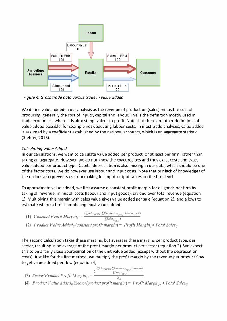
We define value added in our analysis as the revenue of production (sales) minus the cost of producing, generally the cost of inputs, capital and labour. This is the definition mostly used in trade economics, where it is almost equivalent to profit. Note that there are other definitions of value added possible, for example not deducting labour costs. In most trade analyses, value added is assumed by a coefficient established by the national accounts, which is an aggregate statistic (Stehrer, 2013).

Calculating Value AddedIn our calculations, we want to calculate value added per product, or at least per firm, rather than taking an aggregate. However, we do not know the exact recipes and thus exact costs and exact value added per product type. Capital depreciation is also missing in our data, which should be oneof the factor costs. We do however use labour and input costs. Note that our lack of knowledges ofthe recipes also prevents us from making full input-output tables on the firm level.

To approximate value added, we first assume a constant profit margin for all goods per firm by taking all revenue, minus all costs (labour and input goods), divided over total revenue (equation 1). Multiplying this margin with sales value gives value added per sale (equation 2), and allows to estimate where a firm is producing most value added.

The second calculation takes these margins, but averages these margins per product type, per sector, resulting in an average of the profit margin per product per sector (equation 3). We expect this to be a fairly close approximation of the unit value added (except without the depreciation costs). Just like for the first method, we multiply the profit margin by the revenue per product flow to get value added per flow (equation 4).

Figure 4: Gross trade data versus trade in value added

Resulting Value Added DatabaseTo create the final database, the two above mentioned methods were employed to create two estimates of value added per product flow. Each product flow consists of all the sales for 2017 of one producer (the seller) to one client (the buyer) of one product type (HS4 code). Added to the product flows are other pieces of information from this data, such as the total value that the supplier bought of the product that is being sold (which seems the most likely material input), the number of sales in that product flow (so total number of recorded transactions of that product to that client), labour costs and profit shares as defined above. By aggregating per flow, we make the database more manageable without losing much information. The second method of calculating value added assuming constant margin per product per sector gives the most reliable results. As the data is now standardized, firms and products can be compared to one another from the product level up and thus the database is ready to use in economic analysis.

A short analysis comparing the value added database to the macro accounts readily shows the alternative analysis this database offers. Figure 5 shows the production per sector as used in the national accounts4 side by side with the value added based on the EBM sales data. There are some differences to be expected, for example due to the subdivision of 'Other Service Activities' into subsectors in the national accounts. The national accounts total is also around 2.2 billion RWF higher. Less obvious is the radical difference in both the wholesale sector and agricultural sector. For agriculture, some difference is to be expected given that Rwanda has many smallholder farmers which would not show up in EBM data (far below the 20 million RWF VAT-registration threshold). This does however not explain the difference between being a marginal sector and producing around a third of GDP. The huge shift in relative importance of the wholesale sector is also intriguing, though it might indicate that our attempt to calculate value added still overestimates value added by throughput sectors. The last interesting difference, the change in relative size of manufacturing, is however explained by overestimation of throughput sectors.

4 We altered the sector division slightly to fit the sector classification used by the RRA, which we used as the leading category. Most notably, the 'Other Service Activities' is a aggregate heading in the national accounts in which many other service sectors are summed, so we had to drop this to avoid double counting. The national accounts also adds some other accounting factors not used in our analysis.

Figure 5: Value added per sector according to the EBM data using constant margins per sector per product (left, blue) versus production per sector according to the national accounts (right, red)

These discrepancies show the very different view one gets of the economy when using sales data rather than production data, clearly there is a difference in production value versus trade value. It also raises questions which view shows the more accurate image of the economy.

5. Data Output and Sensitivity Analysis

Data cleaningThe database of product flows with value added calculations is vast. With the data now being moreinterpretable, we can properly clean, assess and analyse the final database, which is described in this chapter.

For starters, minor cleaning was carried out. The reason for the cleaning being minor in relation to messy data, is twofold. Firstly, the first cleaning used for the HS4 classification already filtered out some of the really troubling data. Secondly, the item names are incorrect in predictable ways, as opposed to the quantitative data which correctly has very large variation, and is also not normally distributed, as shown later. Meaning that excessive cleaning would result in loss of good data and thus possibly in just as much distortion as the bad data itself.

There was however one clear outlier which had a value of several times the GDP of Rwanda, and some very large negative values. The firms (buyer and supplier) with TINs not found in the tax registration database were dropped. In general, there were many sales with negative values, whichis problematic, as some of these are data errors, but also many are expected to be corrections on earlier sales, when an earlier error was corrected. Removing only the negatives would result in an overestimation, but we were also not able to match all the corrections to the original sale, as names were often different for the corrections. In the aggregate however, at least on the firm level and often on the product level, the negative values should automatically match up to the values that were to be corrected in the first place. We do indeed see in the final database that for productflows and firm aggregates the number of negative values is significantly less. Unfortunately, some negatives remain nonetheless. For some analyses shown here and in the accompanying IGC paper, the negatives had to be dropped prior to analysis, but they are kept in the main database.

An important point when cleaning the dataset is that it is not normally distributed. This makes sense, as there are only a few 'winner firms' which make most of the revenue and profit. Also, firms would not generally have negative turnover values.. This makes the turnover per firm heavily skewed towards 0. On the sales level, small sales are much more frequent than large sales, which istrue for any country, but for a developing nation even more so. Illustrative for this is that in graphing the distribution of the product flows (which are already aggregate values), it is necessary to cut off all values above 100,000 RWF (≈ 115 USD) to have a readable graph, as shown in figure 6.Given that it an earlier IGC study showed that bigger transactions are more likely to get recorded by an EBM and only 5-9% of smaller transactions to consumers are recorded in an EBM, the actual distribution of transaction size is even more skewed(IGC, 2017).

Data outputThe remaining data is described in table 4 with descriptive statistics per firm. After cleaning described earlier, the resulting items were added up into 2.8 million product flows. The resulting database describes all the formal economic activity, totalling roughly 5.2 billion USD in value, by 11,605 different supplier firms and 55,844 client firms and an unrecorded number of consumers. Itshows which product flow has more economic importance to the supplier, both in total value added and in profitability and also shows where the supplier gets its inputs from.

Name Description Mean per firm Max per firm

Number of suppliers Number of supplying firms per firm 14 1,128

Number of buyers Number of buying firms per selling firm (consumers are not recorded)

77 11,140

Sales Worth of sales (RWF) for firms with sales

454,968,747 933,511,091,600

Inputs Total inputs (RWF) of all firms 48,198,636 41,958,338,560

Number of transactions

Total number of item lines registered per firm

5,023 3,526,995

Range of products sold per supplier

Number of different types (HS4 codes) sold per supplying firm

34.6 229

Worth of product flows

Worth (RWF) per product flow, i.e. all sales per type of product per supplier-buyer pair

35,000 907,000,000,000

Product flows per supplier

Number of product flows per supplying firm

219.8 44,150

Products sold per firm

Total quantity of products sold per supplying firm

54,765 56,872,146

Table 4: Descriptive statistics per firm, after cleaning and value added calculation.

Figure 6: Illustrating non-normal distribution: percentage of flows with certain value per product flow (so per product per client-supplier pair). A cut-off at 100.000 RWF is necessary to create a readable graph. Similar graphs can be made for turnover per firm, value per sale, number of sales.

From the output we canreadily draw severalconclusions on importantproducts and successfulsectors. Table 5 shows themost often sold products.Some of these seemunlikely, and might mostlyresult from the machinelearning, such as fittings forlamps. For the otherproducts, it makes sensethat these are oftentraded, generally in smallquantities, such as beer.

Sensitivity analysisThe aggregates of the data seem quite reliable. For the more clear and consistent products, such ascement, the product classification also seems to work well. During analysis however, the product classification seemed to be off more often for less consistent products than was to be expected from the product classification statistics. This is illustrated by many firms making most of their value added on 'machines for working rubber' (code 8477) or 'fittings for lamps' (9405) which seems quite unlikely to be such an important market in Rwanda. It is mostly infrequent large sales (eg cars) or with relatively inconsistent names (eg ink cartridges) which are to be expected to be misclassified. When the machine learning is improved, this might mean large shifts in value added per product, firm and sector. From table 5, we can expect a shift of close to 20 percent once product flows classified as 0 are correctly classified. Adding significant portions of the classifications on 'lamps', 'fittings for lamps' and 'machines for working rubber' and some other classification, we can expect 20-40% of product flows to shift to a different classification.

Another point to address is the sensitivity of the value added part of the database to the method of defining and calculating value added. Stehrer (2012) shows how influential different calculationsof trade in value added can be, and how subsequent policies can be severely affected by wrong calculations. Figure 7 shows the large variance of profit margins per sector between the two ways of calculating. Judging by the spreads per sector for the two methods the method of using a median profit share per product per sector provides a much more realistic and especially more robust method, which is why we chose to primarily use this in analyses throughout the paper.

Table 5: Top 10 product codes in number of flows

Figure 7: Comparing constant profit share across sectors per product (blue, left) versus constant profit margin per firm (red, right) for all available sectors

A final point of attention on the sensitivity of the analysis is the limited cleaning we did on the dataset. As described earlier, this is mostly due to the fact that the data is too vast to manually clean. At the same time, the data has a non-normal distribution, which means conventional cleaning methods would result in throwing away good, valuable data points. Ideally, improvementsare made at the point of data input, meaning the cashiers. Making improvements there will however be hard in practice, though the second version of the EBM, which is more software-based, will likely allow for more improvement. The second version is unfortunately only used by 5-10% of the current firms. Nevertheless, unchecked data errors could be very influential and thoroughly corrupt analyses. Any improvements or checks that could be implemented are thus worth investigating and investing in.

6. Conclusions and Future Applications

This paper set out to set up a useful and convenient firm level sales database to be used for multiple applications. We showed we are able to process the EBM data into a useful and highly valuable database. Though we provided a sound proof of concept, it is also evident that the product classification needs be improved. The most sensible way forward seems to increase the size of the training data. After that, the main challenge is defining and calculating value added. Theactual calculation is relatively easy to execute, but defining value added and getting relevant data will remain a point of attention, though there is not necessarily only one correct way of doing this.Once these challenges are addressed, there are many applications for this unique database. Spray and Steenbergen’s work on backward linkages shows that we are able to use the final dataset for important and valuable economic analysis, which cannot be conducted without this database. Theapplications are really whatever anyone can think of, but we have already started on a list with

Identifying potential for backward linkagesThe EBM data can be used to identify successful products which are domestically produced, and compare these to import data. When products which are domestically produced, but also imported by many firms, government actors such as RDB could use such a dataset to find out what constraints are for using domestic producers.

Identifying successful firms and sectors and unsuccessful counterpartsIn a similar way as identifying potential for backward linkages, both successful and unsuccessful firms can be identified. After identification, they could be linked to one another to share best practices and create a platform to increase cooperation. This could also be used to supplement work on stimulating potential for backward linkages, by using the platform to tackle constraints for large multinationals.

Identify sectors and products with too few or too many producersThe same database can provide insight into the number of producers of certain products. The Rwandan government could use such information to stimulate or slow down firms moving into a certain sector, helping the private sector to develop where the most potential is.

Improve data on sector classificationWith a rich dataset on what products a firm is buying and selling, the Rwandan government (RRA, NISR) could use clustering algorithms to increase the accuracy of sector classification of taxpayers. A better classification increases the quality of the national statistics, but also helps in aiming policies at certain sectors. Not too long ago, this data was only self-reported, resulting in data without much information. More recently the RRA has been putting a lot of work into improving this classification manually, but this might be augmented by implementing a machine learning algorithm. Please refer to the second annex of this paper on first work on automated sector classification

Use in data driven auditingSimilar to improving sector classification, knowing what a firm buys and sells helps to target firms which need to be audited more accurately, greatly reducing the cost of tax compliance for both theRRA as well as complying taxpayers. The RRA could create a system targeting firms which are selling products according to their EBM data which are highly unlikely in their sector. As Steenbergen (2017) shows, EBMs can be of great influence of improving tax compliance, and the potential worth of improved VAT compliance specifically is vast.

Infrastructure prioritisationWhen location data is added to the dataset, for example GPS data of the EBMs, the database couldalso geographically map trade. Adding to this that good product classification also indicates where more heavy materials are often transported, such a database would allow for very detailed cost benefit analysis of infrastructural projects. Such analyses are very helpful in prioritising which projects will give the highest return.

Creation of hubs by identifying similar or interdependent firmsSimilar analysis facilitates the creation of hubs of similar firms or firms which are close to another in the value chain. Hubs with firms in the same sector allow for accelerated innovation, while interdependent firms could greatly reduce transport and transaction costs. Hubs are also often attractive for new investors.

Early warning systems for natural hazards or epidemicsA completely different application would be to use the data of which products are being sold to inform the government of epidemics or disaster before the actual onset, when the data is processed in (near) real-time. For example, picking up a spike in water sales could already indicate a drought before weather data would suggest the same, or a spike in fever-reducing medicines could indicate an epidemic.

ConclusionIn conclusion, with some additional investment into mainly item classification, the EBM data can be utilized in a number of fields and applications, ranging far and wide beyond this list. For some applications, already the non-classified data could prove useful. The government of Rwanda can use all these applications to increase data-driven decision making, resulting into better informed and more efficient policies, at relatively low further costs as the EBMs are already in place. The paper by IGC on potential for backward linkages (Spray and Steenbergen, 2018) shows just how useful this database is. As such, utilizing the EBM dataset to its full potential should be made into apriority.

Literature

Aslam, Aqib, Novta, Natalija and Fabiano Rodrigues-Bastos, 2017. “Calculating Trade in Value Added” IMF working paper, WP/17/178.

Eissa,N., Andrew Zeitlin, A., Karpe, S. and Murray,S., 2014.”Incidence and Impact of Electronic Billing Machines for VAT in Rwanda”. IGC report, Kigali, Rwanda.

IGC, 2017. “Improving EBM adherence: An experimental evaluation of an innovative audit strategy”, IGC Progress report to the Rwanda Revenue Authority, Kigali, Rwanda.

Laterite, 2018. “EBM Data Portal: Classifying Items on EBM Receipts”. Laterite report, commissioned by the IGC and RRA, Kigali, Rwanda.

MINEACOM, 2017. “Made in Rwanda Policy”. Kigali: Ministry of Trade and Industry.

National Institute of Statistics of Rwanda (NISR), 2012. 'The Rwanda Classification Manual, 2012 Edition'.

OECD, 2013. “Working document number 9: Draft Chapter 9 Measuring Trade in Value-Added”, prepared for the Meeting of the Group of Experts on National Accounts.

Spray, J. and Steenbergen, V., 2018. “The Potential for Backward Linkages”, IGC Policy Note, June 2018, Kigali, Rwanda.

Stehrer,R., 2012. “Trade in Value Added and the Value Added in Trade”, World Input Output Database working paper.

Steenbergen, V., 2017. “Reaping the benefits of Electronic Billing Machines: using data-driven toolsto improve VAT compliance”. IGC report, Kigali, Rwanda.

Timmer, M. P., Dietzenbacher, E., Los, B., Stehrer, R. and de Vries, G. J., 2015. "An Illustrated User Guide to the World Input–Output Database: the Case of Global Automotive Production", Review of International Economics, 23: 575–605

Annex 1: Methodology used for the classification of items

IGC commissioned Laterite to create a machine learning algorithm to be able to parse and classify the EBM data. The summary after this part shortly describes the work they have done and the accuracy of the classification. The full report accompanies this paper. Described below is the expansion of the training data that we did to the Laterite work, as well as a short list of customized HS codes not normally included in HS databases.

The Laterite report concludes at a training set of roughly 10,000 randomly picked, clustered and hand-tagged item names. After running the classification algorithm on the actual data, the accuracy seemed less (note that this was our own intuition) than expected from the accuracy reports. As an example, many common items like rice, water and beer were classified as 'telephone sets'. IGC expanded and improved this set using a snowball approach.

First off, 800 items from the actual data incorrectly classified as telephone sets were semi-randomly selected, re-classified, multiplied 5 times to increase power, and added to the training data. This increased the training set with about 40%, mostly increasing power for common items such as milk, water, beer, rice and sugar. The disadvantage was of course that items which are more difficult to classify were often classified as common items. To counter this, another 250 observations of less common items with little support (about 5-15 occurrences in the training data)were selected from the final data and added to the training data. Finally, another 100 observations were added on items such as services and non-food, which were often classified as 0, so unclassifiable. All these 350 observations were taken from different parts of the final data, to increase the variance within the item names. These 350 items were multiplied 3 times and added to the training data set, which now contained just over 15,000 items, just over 50% bigger than theoriginal.

The accuracy estimated by the algorithm itself increased from about 70% in the Laterite version to around 80% in the new version due to our expanded training data. Eyeballing the second round of classification supported this increase. Note however that due to the copying and non-randomly adding of items, the integrity of the machine learning algorithm might be somewhat compromised.Nevertheless, the accuracy increase was substantial, against minor costs.

To cope with the missing classification of services in the standard HS classification, Laterite and IGCused some of the HS codes above 9800 which are generally reserved for customization (by countries). The extra codes used were:9835 – mail/courier9838 – storage9850 – transportation9943 – hotel and accommodation9970 – Other small services, (engine service, extra service, door lock service, haircuts, security services)

Executive Summary of the report “EBM Data Portal: Classifying Items on EBM Receipts” by Laterite

This project proves that it is technically possible to classify items on EBM receipts against a standard classification. This could open up a range of new types of compliance, economic

and policy analysis for RRA and Government of Rwanda Ministries. The proof-of-concept algorithm correctly classified the item to the correct code 70% of the

time, this is a good performance when considering that there are hundreds of possible classification codes but only one correct classification code for each item. Around 12% of the item data was unclassifiable (e.g. “Dept 01”) or unintelligible (“A B C”) to a human review and not useable for the algorithm. There remain many areas for technical improvements and suggestions have been made on how to improve the performance of the algorithm.

However, implementing and gaining the most benefits from data analysis is not just a technical problem; it requires a strategy for using the model and support across the organization. Therefore while this report focuses on the technical challenges overcome and outstanding in producing the prototype algorithm, the recommended next steps are for RRA to consider the wider requirements needed to implement a Machine Learning model and whether the benefits and costs justify investment in data analysis of EBM item level.

Annex 2: Methodology for automatically classifying firms into sectors

Problem description and potentialFor most economic analyses, having a proper sector classification helps to aggregate firms and data to a convenient level. It also helps in distinguishing firms into main activities and thus products, for example primary potato production in agriculture versus selling warm mashed potatoes in hospitality versus selling (processed) crisps in supermarkets. This is vital information to do a meaningful analysis but is also important information for the RRA itself, as it helps in risk analysis and performance measurement. As an example, common assumption within auditing is that the hospitality sector has lower VAT compliance. Similarly, when the firms' sector can be reliably established, te EBM data can be used to monitor firms more closely automatically, and flag firms showing deviant behaviour. For example, currently, the EBM data with proper product classification could already be used to start flagging firms which buy only water and soda, but sell toys. This type of analysis would still require some work, but could be done without proper sector classification. However, if the sector classification would be improved significantly, any firm selling toys (according to EBM data) which would be in the food production sector (or another unrelated sector) could be flagged for inspection, without the need for analysis and matching of inputs.

The RRA currently has a taxpayer registration with a classification of firms into a 2-digit (one letter) International Standard Industrial Classification (ISIC) code, generally self-reported by the firms during initial registration. The problem with this is that is not very granular, there seem to be quite a bit of mistakes, and mostly, about 40% of the firms are in 'Other Service Activities', which is not very informative. The RRA has worked hard to improve the classification manually by calling firm owners, but making progress is hard, also due to the fact that proper classification is a complex process. Ideally, classification is done using a top-down method of analyzing value-added per extra digit, where the largest share of value added per activity determines the added digit. For a clear description of this process in Rwandan context, see the 'Rwanda Classification Manual' constructedby NISR in 2012.

Potential for improvement of sector classificationGiven that the EBM data set is rich in features and coverage and adds quite a few firm characteristics, we have tried to improve the sector classification by using a machine learning algorithm on the processed EBM data. Theoretically, it should be relatively easy to improve on the current classification, as there are several firm characteristics to distinguish between sectors, integration and place in the value chain. Even more so, such an algorithm might even outperform human classification as it takes into account detailed value added data. Note though that even with a better product classification on the HS4 level, we can seldom distinguish products being rawmaterial or finalized goods.

To start with, on the basis of PAYE,VAT and the taxpayer registration, the dataset already contains number of employees (or rather, total labour cost), name of the firm, location of the firm, total revenue, the main entity activity (sector) description as given by the taxpayer and tax regime for the different taxes. This already describes broadly the type of operation. For example, if a business is located in the centre of Kigali, it is unlikely to be a large farm. Similarly, not many elevator maintenance firms would be primarily based in Nyagatare. The ratio between size and number of employees also already tells us something about capital intensity, as well as just sheer size: there are few automotive retailers with an annual turnover of less than a new car's worth, which is a nontrivial point in Rwanda, as it is roughly the cut-off for being a small enterprise without VAT

obligations in Rwanda (below 20 mln RWF).

However, the EBM data adds a lot of vital information to this already useful set. For example, the data shows number of sales, quantities, value per sale and if the sale was made to a business or a consumer. One would for example expect businesses at the start of the value chain to be almost exclusively selling to other businesses, with mostly few sales of a high value and either high quantity or low quantity but large size per quantity: say weekly shipments of metal to a metal processing firm. Further down the chain, the number of sales increases, as also the number of firms sold (and bought from) increases: the metal processing firm sells to several business, resulting in more sales every week, and maybe even already some sales to consumers. At the end of the chain, say a retailer in (metal) car parts, would see a lot of sales to consumers (but still also asizeable number to other firms), with a much lower value per sale.

Furthermore, the EBM data indicates the size of the range of products sold. A rice farm sells only one HS4 category, or maybe ten if they are more diversified. However, a food retailer easily sells fifty to a hundred categories. Next to the product range, the actual categories should be very similar within sectors: both farms and metal producers might sell maximum ten categories, but theten categories for farms are quite different. So one could already estimate that if a firm has a rangeof ten HS4-categories, it is likely to be around the start of the value chain. But if one of these categories is rice, you can almost certainly exclude the metal producing sector. Similarly, if a business sells over a hundred HS4 categories, and it sells both bread, cleaning products and sport equipment, it is not just a food retailer, but a proper large supermarket.

The figure below shows some practical examples, listed along random value chains, with the discriminating features, which was used to find the practical implications of this theoretical thinking for just the features added by the EBM data.

Meat value chain

Farmer: only B2B, small range of HS4, small number of sales per day,

Meat processor: only B2B , small range of hs4 with typical HS4's for meat, bigger quantities per sale than farmers,

Supermarket: mostly B2C, large range of HS4, large number of small sales

Restaurant: only B2C, small range of HS4, small quantities, large number of sales

Car parts value chain

Steel plant: only B2B, small range of HS4, small quantities, but high unit price

Parts manufacturer: only B2B, small range of HS4, low number of sales, higher quantities than steel plant

Wholesaler: high B2B, possibly large range of HS4, relative low number of sales, with highquantity

Garage: equal B2C as B2B, low quantity, small range of HS4, relative high unit price

Specialized shop: both B2B and B2C, low quantity, small range of HS4 but larger than garage

Retailer selling car parts: Mostly B2c, large range of HS4, low quantities per sale

Machine learning algorithmAlthough the theoretical side seems quite clear cut, putting it into machine learning practice is quite challenging. The most important part is that the correct sectors are generally not easily visible: you have to know a firm to be able to classify it, or you have to be able to compare it on the abovementioned metrics to classify it. Therefore, it is a lot harder to use a normal supervised learning algorithm, as it is a lot harder to create a training set. The most promising and interesting (it will be more informative as it uncovers 'hidden' patterns) approach is therefore using an unsupervised machine learning algorithm, generally a clustering algorithm. However, there are many features to cluster the firms by. Next to the above mentioned features, if one wishes to use the actual HS4 codes sold (not just the range), every HS4 code is a feature with a dummy variable (or the actual number/value of sales), resulting in about 300 features in total for our set. This requires relatively advanced machine learning, as first we need to establish which features are informative. Also, we need to make sure all the features are treated in a similar way: the dummy variables for the HS4 codes as well as the total turnover, despite their large difference in scale and variance. We therefore need to normalize the values first.

For the actual techniques, we used the available Sklearn packages, available freely online. Varying ML techniques were employed to try to find appropriate methods. In general, this was very much atrial and error type of process, with several different combinations of methods within a pipeline, leaving much room for improvement by using a more structured approach.

As the different features (variables) have very differing ranges, it seems wise to start with the Normalizer function before anything else. This normalizes the variables to a 0-1 range, so that the impact per feature is the same. After that, Principal Component Analysis (PCA) was used on different configurations of features to try to find how many features were actually informative. In most configurations, 4-5 features were driving the results, though the other features still had someinformational value.

In general, Kmeans was used as the main clustering algorithm, with n_clusters varied between 10 and 100. Silhouette analysis was used to measure the performance of the different methods, where the maximum silhouette coefficient reached of 0,4 with random features selected out of thedummy HS4 category variables. As a general rule of thumb, most ML-experts view a silhouette coefficient below 0,4-0,5 as highly unreliable, with anything above 0,6-0,7 as being useful for analysis, and above 0,75 as reliable. The maximum value of 0,4 is thus too low to be useful.

Theoretically, one would expect proper results from hierarchical clustering, as this is actually used in the top down approach of the normal ISIC classification systems (start at sectors as 'hunting, agricultural production and fishing', then with subdivision into 'agricultural production' , with a subgroup as 'agricultural production of fruits'). This would result in a low number of groups clustered on a high level, with an increasingly large number of groups at lower levels of clustering. However, most firms got quickly clustered at a low level, without an interpretable reason. For example, a large beverage producer was in a cluster with a cement factory and a supermarket.

Given the high dimensionality, especially with the dummy variables, tSNE seemed a likely alternative, strong in dimensionality reduction. Most of the tSNE graphs however did not show clear clusters, just noise, which was sometimes neatly boundaried (little mixing between clusters), but often just random, such as figure A1.

When using many dummy variables, truncatedSVD can also be helpful, being often used in text analysis. This did improve results somewhat, but not enough to be meaningful, as seen in figure A2.

Figure A1: tSNE map of 30 clusters, with a learning rate of 300.

Figure A2: mapped using SVD and 30 clusters.

For all of these methods, different calibrations (n_clusters, learning_rate, stability rate, minimum cluster size) and set-ups (with and without normalization, using only PCA defined component or disregarding PCA) were tried. This included different variable structures such as with and without dummy variables for HS4 categories, with just numerical variables or also categorical variables converted into numeric. Different subsets within the data were tried, as well as adding the already reclassified ISICs by the RRA. Also excluding the EBM data, relying solely on the quite reliable (but aggregate) data of the other sources. The highest silhouette score was obtained by using a few random HS4 category dummies, with hardly any other (meaningful) variables, shown in figure A3, with a silhouette score of 0,7. This seems to stress the fact that some serious thought has to be putinto this modelling for it to be improved, rather than continuing a trial and error approach.

In summary, sector classification should be very well possible, but our attempt did not show meaningful results. To improve on the classification, the first step would be to improve the productclassification, to ensure meaningful input into the sector classification. When the sector classification approach is improved, it is potentially very informative and useful.

Figure A3: clustering using a small number of random HS4 dummy categories shows the bestresult, but still mostly looks like noise.

Designed by soapbox.co.uk

The International Growth Centre (IGC) aims to promote sustainable growth in developing countries by providing demand-led policy advice based on frontier research.

Find out more about our work on our website www.theigc.org

For media or communications enquiries, please contact mail@theigc.org

Subscribe to our newsletter and topic updates www.theigc.org/newsletter

Follow us on Twitter @the_igc

Contact us International Growth Centre, London School of Economic and Political Science, Houghton Street, London WC2A 2AE