Estimating treatment effect heterogeneity in randomized ... · 2 K. IMAI AND M. RATKOVIC heterogeneity as the degree to which different treatments have differential causal effects

arX

iv:1

305.

5682

v1 [

stat

.AP]

24

May

201

3

The Annals of Applied Statistics

2013, Vol. 7, No. 1, 443–470DOI: 10.1214/12-AOAS593c© Institute of Mathematical Statistics, 2013

ESTIMATING TREATMENT EFFECT HETEROGENEITY INRANDOMIZED PROGRAM EVALUATION1

By Kosuke Imai and Marc Ratkovic

Princeton University

When evaluating the efficacy of social programs and medical treat-ments using randomized experiments, the estimated overall average causaleffect alone is often of limited value and the researchers must investigatewhen the treatments do and do not work. Indeed, the estimation of treat-ment effect heterogeneity plays an essential role in (1) selecting the mosteffective treatment from a large number of available treatments, (2) as-certaining subpopulations for which a treatment is effective or harmful,(3) designing individualized optimal treatment regimes, (4) testing forthe existence or lack of heterogeneous treatment effects, and (5) gen-eralizing causal effect estimates obtained from an experimental sampleto a target population. In this paper, we formulate the estimation ofheterogeneous treatment effects as a variable selection problem. We pro-pose a method that adapts the Support Vector Machine classifier byplacing separate sparsity constraints over the pre-treatment parametersand causal heterogeneity parameters of interest. The proposed methodis motivated by and applied to two well-known randomized evaluationstudies in the social sciences. Our method selects the most effective votermobilization strategies from a large number of alternative strategies, andit also identifies the characteristics of workers who greatly benefit from(or are negatively affected by) a job training program. In our simula-tion studies, we find that the proposed method often outperforms somecommonly used alternatives.

1. Introduction and motivating applications. While the average treat-ment effect can be easily estimated without bias in randomized experiments,treatment effect heterogeneity plays an essential role in evaluating the effi-cacy of social programs and medical treatments. We define treatment effect

Received January 2012; revised September 2012.1Supported by NSF Grant SES–0752050. The proposed methods can be implemented

via open-source software FindIt [Ratkovic and Imai (2012)], which is freely available atthe Comprehensive R Archive Network (http://cran.r-project.org/package=FindIt).This software also contains the results of our empirical analysis.

Key words and phrases. Causal inference, individualized treatment rules, LASSO,moderation, variable selection.

This is an electronic reprint of the original article published by theInstitute of Mathematical Statistics in The Annals of Applied Statistics,2013, Vol. 7, No. 1, 443–470. This reprint differs from the original in paginationand typographic detail.

1

http://arxiv.org/abs/1305.5682v1

http://www.imstat.org/aoas/

http://dx.doi.org/10.1214/12-AOAS593

http://www.imstat.org

http://cran.r-project.org/package=FindIt

http://www.imstat.org

http://www.imstat.org/aoas/

http://dx.doi.org/10.1214/12-AOAS593

2 K. IMAI AND M. RATKOVIC

heterogeneity as the degree to which different treatments have differentialcausal effects on each unit. For example, ascertaining subpopulations forwhich a treatment is most beneficial (or harmful) is an important goal ofmany clinical trials. However, the most commonly used method, subgroupanalysis, is often inappropriate and remains one of the most debated prac-tices in the medical research community [e.g., Rothwell (2005), Lagakos(2006)]. Estimation of treatment effect heterogeneity is also important when(1) selecting the most effective treatment among a large number of availabletreatments, (2) designing optimal treatment regimes for each individual or agroup of individuals [e.g., Manski (2004), Pineau et al. (2007), Moodie, Plattand Kramer (2009), Imai and Strauss (2011), Cai et al. (2011), Gunter, Zhuand Murphy (2011), Qian and Murphy (2011)], (3) testing the existence orlack of heterogeneous treatment effects [e.g., Gail and Simon (1985), Davison(1992), Crump et al. (2008)], and (4) generalizing causal effect estimates ob-tained from an experimental sample to a target population [e.g., Frangakis(2009), Cole and Stuart (2010), Hartman, Grieve and Sekhon (2010), Greenand Kern (2010b), Stuart et al. (2011)]. In all of these cases, the researchersmust infer how treatment effects vary across individual units and/or howcausal effects differ across various treatments.

Two well-known randomized evaluation studies in the social sciences serveas the motivating applications of this paper. Earlier analyses of these datasets focused upon the estimation of the overall average treatment effectsand did not systematically explore treatment effect heterogeneity. First, weanalyze the get-out-the-vote (GOTV) field experiment where many differ-ent mobilization techniques were randomly administered to registered NewHaven voters in the 1998 election [Gerber and Green (2000)]. The origi-nal experiment used an incomplete, unbalanced factorial design, with thefollowing four factors: a personal visit, 7 possible phone messages, 0 to 3mailings, and one of three appeals applied to visit and mailings (civic duty,neighborhood solidarity, or a close election). The voters in the control groupdid not receive any of these GOTV messages. Additional information oneach voter includes age, residence ward, whether registered for a majorityparty, and whether the voter abstained or did not vote in the 1996 election.Here, our goal is to identify a set of GOTV mobilization strategies that canbest increase turnout. Given the design, there exist 193 unique treatmentcombinations, and the number of observations assigned to each treatmentcombination ranges dramatically, from the minimum of 4 observations (vis-ited in person, neighbor/civic-neighbor phone appeal, two mailings, with acivic appeal) to the maximum of 2956 (being visited in person, with anyappeal). The methodological challenge is to extract useful information fromsuch sparse data.

The second application is the evaluation of the national supported work(NSW) program, which was conducted from 1975 to 1978 over 15 sites in theUnited States. Disadvantaged workers who qualified for this job training pro-

ESTIMATING TREATMENT EFFECT HETEROGENEITY 3

gram consisted of welfare recipients, ex-addicts, young school dropouts, andex-offenders. We consider the binary outcome indicating whether the earn-ings increased after the job training program (measured in 1978) comparedto the earnings before the program (measured in 1975). The pre-treatmentcovariates include the 1975 earnings, age, years of education, race, marriagestatus, whether a worker has a college degree, and whether the worker wasunemployed before the program (measured in 1975). Our analysis considerstwo aspects of treatment effect heterogeneity. First, we seek to identify thegroups of workers for whom the training program is beneficial. The programwas administered to the heterogeneous group of workers and, hence, it isof interest to investigate whether the treatment effect varies as a functionof individual characteristics. Second, we show how to generalize the resultsbased on this experiment to a target population. Such an analysis is im-portant for policy makers who wish to use experimental results to decidewhether and how to implement this program in a target population.

To address these methodological challenges, we formulate the estimationof heterogeneous treatment effects as a variable selection problem [see alsoGunter, Zhu and Murphy (2011), Imai and Strauss (2011)]. We propose theSquared Loss Support Vector Machine (L2-SVM) with separate LASSO con-straints over the pre-treatment and causal heterogeneity parameters (Sec-tion 2). The use of two separate constraints ensures that variable selectionis performed separately for variables representing alternative treatments (inthe case of the GOTV experiment) and/or treatment-covariate interactions(in the case of the job training experiment). Not only do these variablesdiffer qualitatively from others, they often have relatively weak predictivepower. The proposed model avoids the ad-hoc variable selection of existingprocedures by achieving optimal classification and variable selection in asingle step [e.g., Gunter, Zhu and Murphy (2011), Imai and Strauss (2011)].The model also directly incorporates sampling weights into the estimationprocedure, which are useful when generalizing the causal effects estimatesobtained from an experimental sample to a target population.

To fit the proposed model with multiple regularization constraints, we de-velop an estimation algorithm based on a generalized cross-validation (GCV)statistic. When the derivation of an optimal treatment regime rather thanthe description of treatment effect heterogeneity is of interest, we can replacethe GCV statistic with the average effect size of the optimal treatment rule[Imai and Strauss (2011), Qian and Murphy (2011)]. The proposed method-ology with the GCV statistic does not require cross-validation and henceis more computationally efficient than the commonly used methods for es-timation of treatment effect heterogeneity such as Boosting [Freund andSchapire (1999), LeBlanc and Kooperberg (2010)], Bayesian additive regres-sion trees (BART) [Chipman, George and McCulloch (2010), Green andKern (2010a)], and other tree-based approaches [e.g., Su et al. (2009), Imaiand Strauss (2011), Lipkovich et al. (2011), Loh et al. (2012), Kang et al.


(2012)]. While most similar to a Bayesian logistic regression with nonin-formative prior [Gelman et al. (2008)], the proposed method uses LASSOconstraints to produce a parsimonious model.

To evaluate the empirical performance of the proposed method, we ana-lyze the aforementioned two randomized evaluation studies (Section 3). Wefind that personal visits are uniformly more effective than any other treat-ment method, while sending three mailings with a civic duty message isthe most effective treatment without a visit. In addition, every mobilizationstrategy with a phone call, but no personal visit, is estimated to have either anegative or negligible positive effect. For the job training study, we find thatthe program is most effective for low-education, high income Non-Hispanics,unemployed blacks with some college, and unemployed Hispanics with somehigh school. In contrast, the program would be least effective when admin-istered to old, unemployed recipients, unmarried whites with a high schooldegree but no college, and high earning Hispanics with no college.

Finally, we conduct simulation studies to compare the performance ofthe proposed methodology with that of various alternative methods (Sec-tion 4). The proposed method admits the possibility of no treatment effectand yields a low false discovery rate, when compared to the nonsparse alter-native methods that always estimate some effects. Despite reductions in falsediscovery, the method remains statistically powerful. We find that the pro-posed method has a comparable discovery rate and competitive predictiveproperties to these commonly used alternatives.

2. The proposed methodology. In this section we describe the proposedmethodology by presenting the model and developing a computationallyefficient estimation algorithm to fit the model.

2.1. The framework. We describe our method within the potential out-comes framework of causal inference. Consider a simple random sample ofN units from population P , with a possibly different target population ofinference P∗. For example, the researchers and policy makers may wish toapply the GOTV mobilization strategies and the job training program to apopulation, of which the study sample is not representative. We consider amulti-valued treatment variable Ti, which takes one of (K + 1) values fromT ≡ {0,1, . . . ,K} where Ti = 0 means that unit i is assigned to the controlcondition. In the GOTV study, we have a total of 193 treatment combina-tions (K = 193), whereas the job training program corresponds to a binarytreatment variable (K = 1). The potential outcome under treatment Ti = tis denoted by Yi(t), which has support Y . Thus, the observed outcome isgiven by Yi = Yi(Ti) and we define the causal effect of treatment t for unit ias Yi(t)− Yi(0).

Throughout, we assume that there is no interference among units, thereis a unique version of each treatment, each unit has nonzero probability


of assignment to each treatment level, and the treatment level is indepen-dent of the potential outcomes, possibly conditional on observed covariates[Rubin (1990), Rosenbaum and Rubin (1983)]. Such assumptions are metin randomized experiments, which are the focus of this paper. Under theseassumptions, we can identify the average treatment effect (ATE) for eachtreatment t, τ(t) = E(Yi(t)−Yi(0)). In observational studies, additional dif-ficulty arises due to the possible existence of unmeasured confounders.

One commonly encountered problem related to treatment effect hetero-geneity requires selecting the most effective treatment from a large numberof alternatives using the causal effect estimates from a finite sample. That is,we wish to identify the treatment condition t such that τ(t) is the largest,that is, t = argmaxt′∈T τ(t′). We may also be interested in identifying asubset of the treatments whose ATEs are positive. When the number oftreatments K is large as in the GOTV study, a simple strategy of subset-ting the data and conducting a separate analysis for each treatment suffersfrom the lack of power and multiple testing problems.

Another common challenge addressed in this paper is identifying groupsof units for which a treatment is most beneficial (or most harmful), as in thejob training program study. Often, the number of available pre-treatmentcovariates, Xi ∈X , is large, but the heterogeneous treatment effects can becharacterized parsimoniously using a subset of these covariates, Xi ∈ X ⊂ X .This problem can be understood as identifying a sparse representation ofthe conditional average treatment effect (CATE), using only a subset ofthe covariates. We denote the CATE for a unit with covariate profile x asτ(t; x) = E(Yi(t)− Yi(0) | Xi = x), which can be estimated as the difference

in predicted values under Ti = t and Ti = 0 with Xi = x. The sparsity incovariates greatly eases interpretation of this model.

We next turn to the description of the proposed model that combines op-timal classification and variable selection to estimate treatment effect het-erogeneity. For the remainder of the paper, we focus on the case of binaryoutcomes, that is, Y = {0,1}. However, the proposed model and algorithmcan be extended easily to nonbinary outcomes by modifying the loss func-tion. We choose to model binary outcomes with the L2-SVM to illustrateour proposed methodology because it presents one of the most difficult casesfor implementing two separate LASSO constraints. As we discuss below, ourmethod can be simplified when the outcome is nonbinary (e.g., continuous,counts, multinomial, hazard) or the causal estimand of interest is character-ized on a log-odds scale (with a logistic loss). In particular, readily availablesoftware can be adapted to handle these cases [Friedman, Hastie and Tib-shirani (2010)].

2.2. The model. In modeling treatment effect heterogeneity, we trans-form the observed binary outcome to Y ∗

i = 2Yi − 1 ∈ {±1}. We then relate

the estimated outcome Yi ∈ {±1} and the estimated latent variable Wi ∈ℜ,


as

Yi = sgn (Wi) where Wi = µ+ β⊤Zi + γ⊤Vi,

Zi is an LZ dimensional vector of treatment effect heterogeneity variables,and Vi is an LV dimensional vector containing the remaining covariates. Forexample, when identifying the most efficacious treatment condition amongmany alternative treatments, Zi would consist of K indicator variables (e.g.,different combinations of mobilization strategies), each of which is repre-senting a different treatment condition. In contrast, Vi would include pre-treatment variables to be adjusted (e.g., age, party registration, turnout his-tory). Similarly, when identifying groups of units most helped (or harmed)by a treatment, Zi would include variables representing interactions betweenthe treatment variable (e.g., the job training program) and the pre-treatmentcovariates of interest (e.g., age, education, race, prior employment statusand earnings). In this case, Vi would include all the main effects of the pre-treatment covariates. Thus, we separate the causal heterogeneity variablesof interest from the rest of the variables. We do not impose any restric-tion between main and interaction effects because some covariates may notpredict the baseline outcome but do predict treatment effect heterogeneity.Finally, we choose the linear model because it allows for easy interpretationof interaction terms. However, the researchers may also use the logistic orother link function within our framework.

In estimating (β, γ), we adapt the support vector machine (SVM) clas-sifier and place separate LASSO constraints over each set of coefficients[Vapnik (1995), Tibshirani (1996), Bradley and Mangasarian (1998), Zhang(2006)]. Our model differs from the standard model by allowing β and γ tohave separate LASSO constraints. The model is motivated by the qualita-tive difference between the two parameters, and also by the fact that oftencausal heterogeneity variables have weaker predictive power than other vari-ables. Specifically, we formulate the SVM as a penalized squared hinge-lossobjective function (hereafter L2-SVM) where the hinge-loss is defined as|x|+ ≡max(x,0) [Wahba (2002)]. We focus on the L2-SVM, rather than theL1-SVM, because it returns the standard difference-in-means estimate forthe treatment effect in the absence of pre-treatment covariates.

With two separate l1 constraints to generate sparsity in the covariates,our estimates are given by

(β, γ) = argmin(β,γ)

n∑

i=1

wi · |1−Y ∗i ·(µ+β⊤Zi+γ⊤Vi)|

2++λZ

LZ∑

j=1

|βj |+λV

LV∑

j=1

|γj|,

where λZ and λV are pre-determined separate LASSO penalty parametersfor β and γ, respectively, and wi is an optional sampling weight, which maybe used when generalizing the results obtained from one sample to a targetpopulation.


Our objective function is similar to several existing LASSO variants butthere exist important differences. For example, the elastic net introducedby Zou and Hastie (2005) places the same set of covariates under both aLASSO and ridge constraint to help reduce mis-selections among correlatedcovariates. In addition, the group LASSO introduced by Yuan and Lin (2006)groups different levels of the same factor together so that all levels of afactor are selected without sacrificing rotational invariance. In contrast, theproposed method places separate LASSO constraints over the qualitativelydistinct groups of variables.

2.3. Estimating heterogeneous treatment effects. The L2-SVM offers twodifferent means to estimate heterogeneous treatment effects. First, we canpredict the potential outcomes Yi(t) directly from the fitted model and esti-mate the conditional treatment effect (CTE) as the difference between thepredicted outcome under the treatment status t and that under the controlcondition, that is, δ(t; Xi) =

12(Yi(t)− Yi(0)). This quantity utilizes the fact

that the L2-SVM is an optimal classifier [Lin (2002), Zhang (2004)]. Sec-ond, we can also estimate the CATE. To do this, we interpret the L2-SVMas a truncated linear probability model over a subinterval of [0,1]. While itis known that the SVM does not return explicit probability estimates [Lin(2002), Lee, Lin and Wahba (2004)], we follow work that transforms the

values Wi(t) to approximate the underlying probability [Franc, Zien andScholkopf (2011), Sollich (2002), Platt (1999), Menon et al. (2012)]. Specif-

ically, let W ∗i (t) denote the predicted value Wi(t) truncated at positive and

negative one. We estimate the CATE as the difference in truncated values of

the predicted outcome variables, that is, τ(t; Xi) =12(W

∗i (t)−W ∗

i (0)). Whilethis CATE estimate is not precisely a difference in probabilities, the methodprovides a useful approximation and returns sensible results that comportwith probabilistic estimates of the CATE. With an estimated CATE foreach covariate profile, the CATE for any covariate profile can be estimatedby simply aggregating these estimates among corresponding observations.

2.4. The estimation algorithm. Our algorithm proceeds in three steps:the data are rescaled, the model is fitted for a given value of (λZ , λV ), andeach fit is evaluated using a generalized cross-validation statistic.

Rescaling the covariates. LASSO regularization requires rescaling covari-ates [Tibshirani (1996)]. Following standard practice, we standardize all pre-treatment main effects by centering them around the mean and dividingthem by standard deviation. Higher-order terms are recomputed using thesestandardized variables. For causal heterogeneity variables, we do not stan-dardize them when they are indicator variables representing different treat-ments. When they represent the interactions between a treatment indica-tor variable and pre-treatment covariates, we interact the (unstandardized)treatment indicator variable with the standardized pre-treatment variables.


Fitting the model. The L2-SVM is fitted through a series of iteratedLASSO fits, based on the following two observations. First, we note that

for a given outcome Y ∗i ∈ {±1}, |1− Y ∗

i Wi|2+ = (Y ∗

i − Wi)2 · 1{1 ≥ Y ∗

i Wi}.Thus, the SVM is a least squares problem on a subset of the data. Second,for a given value of {λβ , λγ}, rescaling Z and V allows the objective functionto be written as a LASSO problem, with a tuning parameter of 1, as

n∑

i=1

wi · |Y∗i − (µ+ β⊤Zi + γ⊤Vi)|

2+ +

LZ∑

j=1

|βj |+LV∑

j=1

|γj |,

where β = λβ · β, γ = λγ · γ, Zi = Zi/λβ , and Vi = Vi/λγ .This allows a fitting strategy via the efficient LASSO algorithm of Fried-

man, Hastie and Tibshirani (2010). Specifically, each iteration of our algo-rithm consists of fitting a model on the set of “active” observations A =

{i : 1 ≥ Y ∗i Wi} and updating this set. We now describe the proposed algo-

rithm in greater detail. First, the values of tuning parameters are selected,λ = {λβ, λγ}. We then select the initial values of the coefficients and fit-

ted values as follows, (β(0), γ(0)) = 0 and Y(0)i = 0 for all i. This places all

observations in the initial active set, so that A(0) = {1, . . . , n}.

Next, for each iteration k = 1,2, . . . , let A(k) = {i : 1≥ YiW(k−1)i } denote

the set of active observations, and a(k) = |A(k)| represent the number of ob-

servations in this set. Define Z(k)i and V

(k)i as the centered versions of Zi and

Vi (around their respective mean), respectively, using only the observations

in the current active set A(k). Similarly, we use Y(k)i to denote the centered

value of Y ∗i using only the observations in A(k). Then, at each iteration k,

the algorithm progresses in three steps. We update the LASSO coefficients as

(β(k), γ(k))

= argmin(β,γ)

{1

a(k)

∑

i∈A(k)

(Y(k)i − β⊤Z

(k)i − γ⊤V

(k)i )2 +

LZ∑

j=1

|βj |+

LV∑

j=1

|γj |

}.

The fitted value is updated as W(k)i = µ(k) + β(k)⊤Zi + γ(k)

⊤

Vi where the

intercept is µ(k) = 1a(k)

∑i∈A(k)(Y ∗

i − β(k)⊤Zi − γ(k)⊤

Vi). These steps are re-peated until (β, γ) converges.

Work concurrent to ours has developed an algorithm for the regulariza-tion path of the L2-SVM [Yang and Zou (2012)]. Future work can combineour work and that of Yang and Zou (2012) in order to estimate the whole“regularization surface” implied by a model with two constraints.

Selecting the optimal values of the tuning parameters. We choose the op-timal values of the tuning parameters, {λZ , λV }, based on a generalizedcross-validation (GCV) statistic [Wahba (1990)], so that the model fit is


balanced against model dimensionality. The number of nonzero elementsof |β|0 + |γ|0 = l provides an unbiased degree-of-freedom estimate for theLASSO [Zou, Hastie and Tibshirani (2007)]. Our GCV statistic is definedover the observation in the active set A, as follows:

V (λZ , λV ) =1

n(1− l/a)2

∑

i∈A

(Y ∗i − Wi)

2 =1

n(1− l/a)2

n∑

i=1

|1− Y ∗i Wi|

2+,

where the second equality follows from the fact that the observations outside

of A does not affect the model fit, that is, |1− Y ∗i Wi|

2+ = 0 for i /∈A.

Given this GCV statistic, we use an alternating line search to find theoptimal values of the tuning parameters. First, we fix λZ at a large value,for example, e10, effectively setting all causal heterogeneity parameters tozero [Efron et al. (2004)]. Next, λV is evaluated along the set of widelyspaced grids, for example, log(λV ) ∈ {−15,−14, . . . ,10}, with the value pro-ducing the smallest GCV statistic selected. Given the current estimate ofλV , λZ is evaluated along the set of widely spaced grids, for example,log(λV ) ∈ {−15,−14, . . . ,10}, and the λV that produces the smallest GCVstatistic is selected. We alternate in a line search between the two parametersto convergence. After convergence, the radius is decreased based on theseconverged parameter values, and the precision is increased to the desiredlevel, for example, 10−4. The final estimates of coefficients are estimatedgiven the converged value of (λZ , λV ).

The use of this GCV statistic is reasonable when exploring the degreeto which the treatment effects are heterogeneous. However, if the goal isto derive the optimal treatment rule, the researchers may wish to directlytarget a particular measure of the performance of the learned policy. Forexample, following Imai and Strauss (2011) and Qian and Murphy (2011),we could use the largest average treatment effect as the statistic (knownas “value statistic”) for cross-validation. In addition to its computationalburden, one practical difficulty of cross-validation based on the value statis-tic is that when the total number of causal heterogeneity variables is largeand the sample size is relatively small as in our applications, we may nothave many observations in the test sample that actually received the sametreatment as the one prescribed by the optimal treatment rule. In addition,the training sample may have empty cells so that they do not predict treat-ment effects for some individuals in the test set. This makes it difficult toapply this procedure in some situations. The use of the GCV statistic is alsocomputationally efficient as it avoids cross-validation.

Comparing computation times across competitors is difficult, as they canvary dramatically depending on the number of cross-validating folds (Boost-ing, LASSO), iterations (Boosting), the number of MCMC draws and num-ber of trees (BART), and desired precision in estimating the tuning pa-rameters (LASSO, SVM). The general pattern from our simulations is that


the computational time for the proposed method is significantly greaterthan the Bayesian GLM, tree, and the cross-validated logistic LASSO witha single constraint. It is comparable to BART and significantly less thancross-validated boosting.

Finally, in a recent paper, Zhao et al. (2012) propose a method thatis related to ours. There are several important differences between the twomethods. First, we are primarily interested in feature selection using LASSOpenalties, whereas Zhao et al. focus on prediction using an l2 penalty. Whilewe use a simple parametric model with a large number of features, Zhao et al.place their method within a nonparametric, reproducing kernel framework.In kernelizing the covariates, they achieve better prediction but at the cost ofdifficulty in interpreting precisely which features are driving the treatmentrule. Second, we use two separate LASSO penalties for causal heterogeneityvariables and pre-treatment covariates, whereas Zhao et al. do not make thisdistinction. Third, our tuning parameter is a GCV statistic, which eliminatesthe computational burden of cross-validation as used by Zhao et al.

3. Empirical applications. In this section we apply the proposed methodto two well-known field experiments in the social sciences.

3.1. Selecting the best get-out-the-vote mobilization strategies. First, weanalyze the get-out-the-vote (GOTV) field experiment where 69 mobiliza-tion techniques were randomly administered to registered New Haven votersin the 1998 election [Gerber and Green (2000)]. It is known in the GOTVliterature that there is substantial interference among voters in the samehousehold [Nickerson (2008)]. Thus, to avoid the problem of possible inter-ference between voters, we focus on 14,774 voters in single voter householdswhere 5269 voters of them belong to the control group and hence did notreceive any of these GOTV messages. Addressing this interference issue fullyrequires an alternative experimental design where the treatment conditionscorrespond to different number of voters within the same household whoreceive the GOTV message (our method is still applicable to the data fromthis experimental design because it can handle multi-valued treatments).For the purpose of illustration, we also ignore the implementation problemsdocumented in Imai (2005) and analyze the most recent data set.

In our specification, the causal heterogeneity variables Zi include the bi-nary indicator variables of 192 treatment combinations, that is, KZ = 192.We include a set of noncausal variables Vi, which consist of the main effectterms of four pre-treatment covariates (age, member of a majority party,voted in 1996, abstained in 1996), their two-way interaction terms, and thesquare of the age variable, that is, KV = 10.

Of the 192 possible treatment effect combinations, 15 effects are estimatedas nonzero (see Table 5 in Appendix). As these coefficients range from maineffects to four-way interactions, they are difficult to interpret. Instead, we


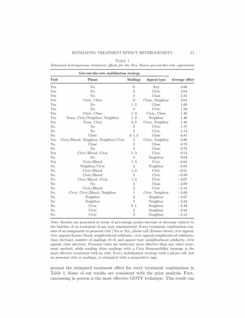
Table 1

Estimated heterogeneous treatment effects for the New Haven get-out-the-vote experiment

Get-out-the-vote mobilization strategy

Visit Phone Mailings Appeal type Average effect

Yes No 0 Any 3.06Yes No 3 Civic 2.64Yes No 3 Close 2.31Yes Civic, Close 0 Close, Neighbor 2.04Yes No 1–2 Close 1.60Yes No 3 Civic 1.50Yes Civic, Close 1–3 Civic, Close 1.46Yes None, Civic/Neighbor, Neighbor 1–2 Neighbor 1.46Yes None, Civic 0,2 Civic, Neighbor 1.46No No 3 Civic 1.17No No 2 Civic 1.14No Close 0,1,3 Close 0.81Yes Civic/Blood, Neighbor, Neighbor/Civic 3 Civic, Neighbor 0.80No Close 2 Close 0.74No No 3 Close 0.70Yes Civic/Blood, Civic 1–3 Civic 0.53No No 3 Neighbor 0.04Yes Civic/Blood 1–3 Civic −0.64No Neighbor/Civic 3 Neighbor −0.65No Civic/Blood 1,3 Civic −0.91No Civic/Blood 2 Civic −0.99No Civic/Blood, Civic 1,3 Civic −2.07No No 2 Close −2.08No Civic/Blood 2 Civic −2.14No Civic, Civic/Blood, Neighbor 1 Civic, Neighbor −2.60No Neighbor 2 Neighbor −2.67No Neighbor 3 Neighbor −3.24No Civic 0–1 Neighbor −3.49No Civic 2 Neighbor −3.56No Civic 3 Neighbor −4.12

Note: Results are presented in terms of percentage points increase or decrease relative tothe baseline of no treatment of any type administered. Every treatment combination con-sists of an assignment to personal visit (Yes or No), phone call (Donate blood, civic appeal,civic appeal/donate blood, neighborhood solidarity, civic appeal/neighborhood solidarity,close election), number of mailings (0–3) and appeal type (neighborhood solidarity, civicappeal, close election). Personal visits are uniformly more effective than any other treat-ment method, while sending three mailings with a Civic Responsibility message is themost effective treatment with no visit. Every mobilization strategy with a phone call, butno personal visit or mailings, is estimated with a nonpositive sign.

present the estimated treatment effect for every treatment combination inTable 1. Some of our results are consistent with the prior analysis. First,canvassing in person is the most effective GOTV technique. This result can


be obtained even from a simple use of the difference-in-means estimator(estimated 2.69 percentage point with t-statistic of 2.68). Second, every mo-bilization strategy that consists of a phone call and no personal visit isestimated with a nonpositive sign, suggesting that the marginal effect ofa phone call is either zero or slightly negative. Most prominently, phonemessages with a neighborhood appeal or civic appeal decrease turnout.

The proposed method also yields finer findings than the existing analy-ses. For example, since personal canvassing is expensive, campaigns may beinterested in the most effective treatment that does not include canvassing.We find that three mailings with a civic responsibility message and no phonecalls or personal visits increase turnout marginally by 1.17 percentage point.This result is similar to the one independently obtained in another study[Gerber, Green and Larimer (2008)]. Three mailings with other appeals pro-duce smaller effects (1.17 and 0.04 percentage point increase, resp.).

Finally, the proposed method, upon considering all possible treatments,produces clear prescriptions. First, in the presence of canvassing, any addi-tional treatment (phone call, mailing) will lessen the canvassing’s effective-ness. If voters are canvassed, they should not receive additional treatments.Second, if voters are not canvassed, they should be targeted with three mail-ings with a civic duty appeal. Any other treatment combination will be lesscost-effective, and may even suppress turnout.

3.2. Identifying workers for whom job training is beneficial. Next, weapply the proposed methodology to the national supported work (NSW)program. Our analysis focuses upon the subset of these individuals previ-ously used by other researchers [LaLonde (1986), Dehejia and Wahba (1999)]where the (randomly selected) treatment and control groups consist of 297and 425 such workers, respectively. We consider two aspects of treatmenteffect heterogeneity. First, we seek to identify the groups of workers forwhom the training program is beneficial. The program was administered toa heterogeneous group of workers and, hence, it is of interest to investigatewhether the treatment effect varies as a function of individual characteris-tics. Second, we show how to generalize the results based on this experimentto a target population. Such an analysis is important for policy makers whowish to use experimental results to decide whether and how to implementthis program in a target population.

For illustration, we generalize the experimental results to the 1978 panelstudy of income dynamics (PSID), which oversamples low-income individ-uals. Within this PSID sample, we focus on 253 workers who had beenunemployed at some point in the previous year to avoid severe extrapola-tion. This subsample is labeled PSID-2 in Dehejia and Wahba (1999). Thedifferences across the two samples are substantial. The PSID respondentsare on average older (36 vs. 24 years old) and more likely to be married (74%vs. 16%) and have a college degree (50% vs. 22%) than NSW participants.


The proportion of blacks in the PSID sample (40%) is much less than in theNSW sample (80%). In addition, on average, PSID respondents earned moreincome ($7600) than NSW participants ($3000). All differences, except forproportion Hispanic, are statistically significant at the 5% level.

In our model, the matrix of noncausal variables, V , consists of 45 pre-treatment covariates. These include the main effects of age, years of educa-tion, and the log of one plus 1975 earnings, as well as binary indicators forrace, marriage status, college degree, and whether the individual was unem-ployed in 1975. We also use square terms for age and years of education,and every possible two-way interactions among the pre-treatment covariatesare included. The matrix of causal heterogeneity variables Z includes thebinary treatment and interactions between this treatment variable and eachof the 39 pre-treatment covariates. This yields KZ = 45 and KV = 44.

Using this specification, we first fit the model to the NSW sample toidentify the subpopulations of workers for whom the job training programis beneficial. Second, we generalize these results to the PSID sample andestimate the ATE and CATE for these low-income workers. Unfortunately,sampling weights are not available in the original data and, hence, for thepurpose of illustration, we construct them by fitting a BART model, usingV as predictors [Hill (2011)]. We then take the inverse estimated probabil-ity of being in the NSW sample as the weights for the proposed method[Stuart et al. (2011)]. To facilitate comparison between the unweighted andweighted models, we standardize the weights to have a mean equal to one.A weight greater than one signifies an observation that is weighted morehighly in the PSID model than in the NSW model. This allows us to as-sess the extent to which differences in identified heterogeneous effects reflectunderlying differences in the covariate distributions between the NSW andPSID samples.

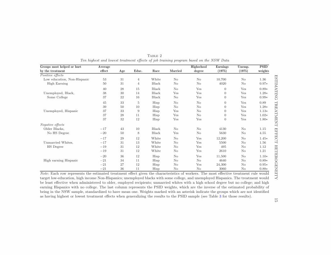
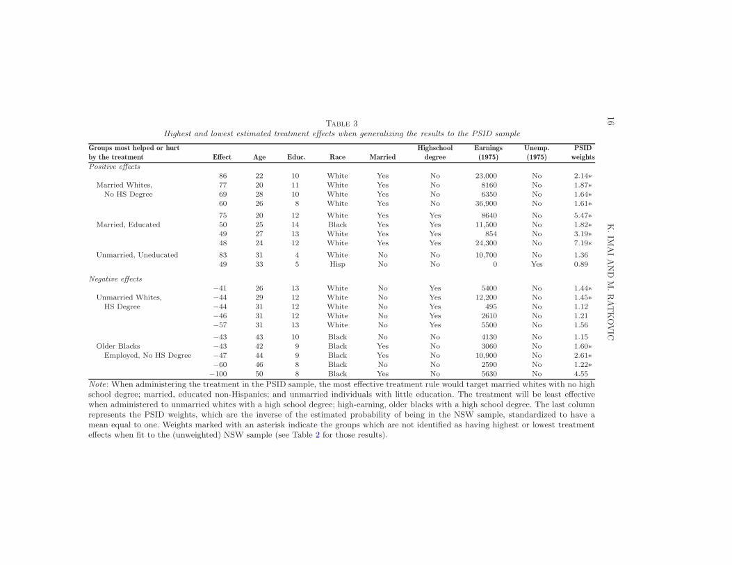
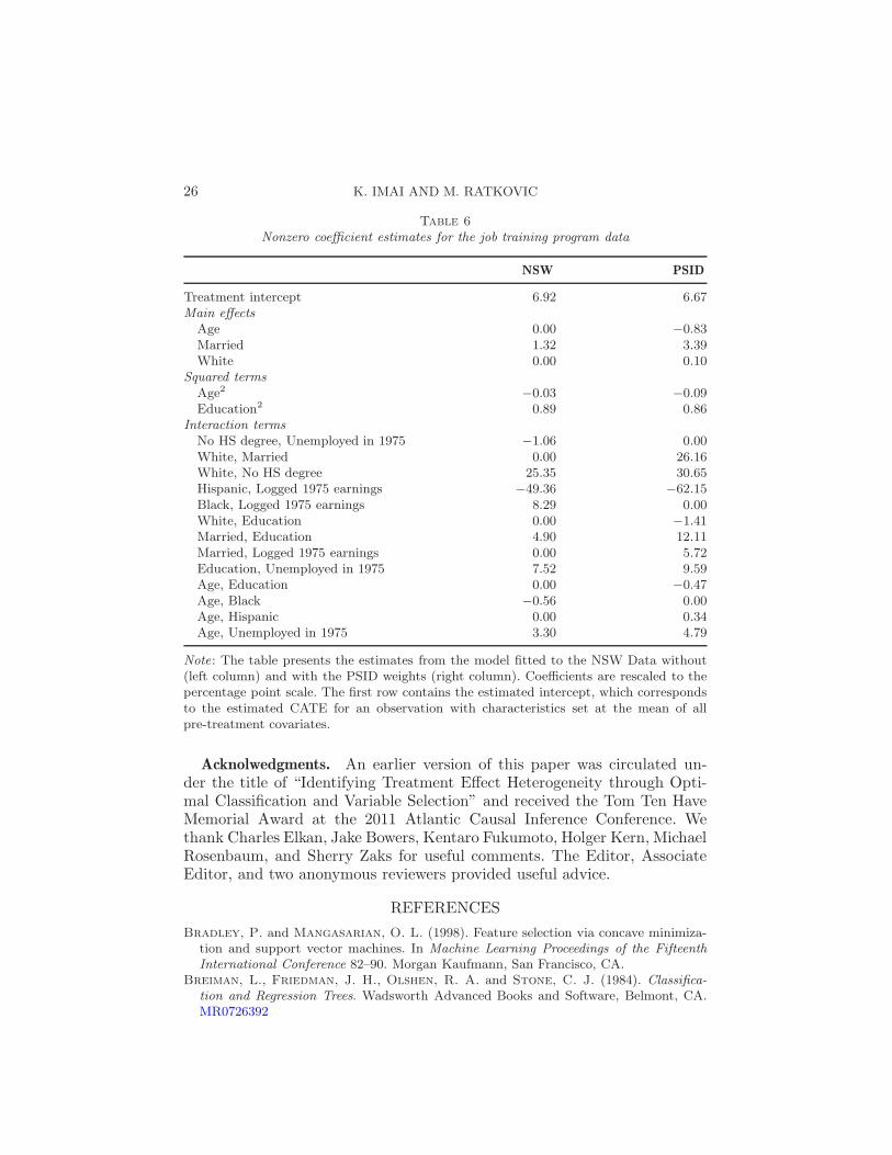
After fitting the model to the unweighted and weighted NSW samples,the CATE is estimated using the covariate value of each observation, thatis, τ(1,Xi). The sample average of these CATEs yields an ATE estimate of7.61 and 4.61 percentage points for the NSW and PSID samples, respec-tively. Nonzero coefficients from the fitted models are shown in Table 6 ofthe Appendix. As with the previous example, interpreting high order inter-actions is difficult. Thus, we present the groups of workers who are predictedto experience the ten highest and lowest treatment effects of the job train-ing program in the NSW (Table 2) and PSID sample (Table 3). The groupsmost helped, and hurt, by the treatment were identified by matching theobservations in these tables to the nonzero coefficients.

Across both tables, unemployed Hispanics and highly educated, low-earningnon-Hispanics are predicted to benefit from the program. Similarly, workerswho were older and employed and whites with a high school degree are iden-tified as those who are negatively affected by the program. Weights markedwith asterisks in each table indicate heterogeneous effects that are not iden-


tified in the other table. For example, unemployed Blacks with some collegeare identified as beneficiaries only in Table 2, while married whites with nohigh school degree only appear in Table 3. This difference is explained by thefact that unemployed blacks with some college make up 2.7% of the NSWsample but only 0.4% of the PSID sample. Similarly, married whites with nohigh school degree make up 15.8% of the PSID sample and are identified inTable 3, but only make up 0.1% of the NSW sample and are not identified inTable 2. Indeed, when generalizing the results to a different population, largegroups in that population are more likely to be selected for heterogeneoustreatment effects. Weighting allows us to efficiently estimate heterogeneoustreatment effects in a target population.

4. Simulation studies. In this section we conduct two simulation studiesto evaluate the performance of the proposed method relative to the com-monly used methods: BART (R package bayestree), Bayesian logistic re-gression with a noninformative prior (R package arm), Conditional InferenceTrees [Hothorn, Hornik and Zeileis (2006); R package party], Boosting withthe number of iterations selected by cross-validation (as implemented in Rpackage ada), and logistic regression with a single LASSO constraint andcross-validation on the “value” statistic [Qian and Murphy (2011); R pack-age glmnet]. The first set of simulations corresponds to the situation wherethe goal is to select a set of the most effective treatments among manyalternatives. The second set considers the case where we wish to identifya subpopulation of units for which a treatment is most effective. In bothcases, we assume that the treatment Ti is independent of the observed pre-treatment covariates Xi. The logistic LASSO method is only applied to thesecond set of simulations for the reason mentioned in Section 2.4. Finally,for each scenario, we examine 4 different sample sizes between 250 and 5000and run 1000 simulations.

4.1. Identifying best treatments from a large number of alternatives. Weconduct simulations for selecting a set of the best treatments among alarge number of available treatments. We use two settings, one with thecorrect model specification and the other with misspecified models, whereun-modeled nonlinear terms are added to the data generating process. In thesimulations with correct model specification, we have one control condition,49 distinct treatment conditions, and 3 pre-treatment covariates. That is,Zi consists of 49 treatment indicator variables and Vi is a vector of 3 pre-treatment covariates plus an intercept, that is, LZ = 49 and LV = 4. Among49 treatments, 3 of them have substantive effects; the ATE is approximatelyequal to 7, 5, and −3 percentage points, respectively. The remaining 46treatment indicator variables have nonzero but negligible effects, with theaverage effect sizes ranging within ±1 percentage point. In contrast, all pre-treatment covariates are assumed to have substantial predictive power.

ESTIM

ATIN

GTREATMENT

EFFECT

HETEROGENEIT

Y15

Table 2

Ten highest and lowest treatment effects of job training program based on the NSW Data

Groups most helped or hurt Average Highschool Earnings Unemp. PSID

by the treatment effect Age Educ. Race Married degree (1975) (1975) weights

Positive effects

Low education, Non-Hispanic 53 31 4 White No No 10,700 No 1.36High Earning 50 31 4 Black No No 4020 No 0.97∗

40 28 15 Black No Yes 0 Yes 0.89∗Unemployed, Black, 38 30 14 Black Yes Yes 0 Yes 1.28∗

Some College 37 22 16 Black No Yes 0 Yes 0.99∗

45 33 5 Hisp No No 0 Yes 0.8939 50 10 Hisp No No 0 Yes 1.28∗

Unemployed, Hispanic 37 33 9 Hisp Yes No 0 Yes 1.13∗37 28 11 Hisp Yes No 0 Yes 1.02∗37 32 12 Hisp Yes Yes 0 Yes 1.80∗

Negative effects

Older Blacks, −17 43 10 Black No No 4130 No 1.15No HS Degree −20 50 8 Black Yes No 5630 No 4.55

−17 29 12 White No Yes 12,200 No 1.45∗Unmarried Whites, −17 31 13 White No Yes 5500 No 1.56

HS Degree −19 31 12 White No Yes 495 No 1.12−19 31 12 White No Yes 2610 No 1.21

−20 36 12 Hisp No Yes 11,500 No 1.10∗High earning Hispanic −21 34 11 Hisp No No 4640 No 0.89∗

−21 27 12 Hisp No Yes 24,300 No 0.95∗−21 36 11 Hisp No No 3060 No 0.88∗

Note: Each row represents the estimated treatment effect given the characteristics of workers. The most effective treatment rule wouldtarget low-education, high income Non-Hispanics; unemployed blacks with some college, and unemployed Hispanics. The treatment wouldbe least effective when administered to older, employed recipients; unmarried whites with a high school degree but no college; and highearning Hispanics with no college. The last column represents the PSID weights, which are the inverse of the estimated probability ofbeing in the NSW sample, standardized to have mean one. Weights marked with an asterisk indicate the groups which are not identifiedas having highest or lowest treatment effects when generalizing the results to the PSID sample (see Table 3 for those results).

16

K.IM

AIAND

M.RATKOVIC

Table 3

Highest and lowest estimated treatment effects when generalizing the results to the PSID sample

Groups most helped or hurt Highschool Earnings Unemp. PSID

by the treatment Effect Age Educ. Race Married degree (1975) (1975) weights

Positive effects

86 22 10 White Yes No 23,000 No 2.14∗Married Whites, 77 20 11 White Yes No 8160 No 1.87∗

No HS Degree 69 28 10 White Yes No 6350 No 1.64∗60 26 8 White Yes No 36,900 No 1.61∗

75 20 12 White Yes Yes 8640 No 5.47∗Married, Educated 50 25 14 Black Yes Yes 11,500 No 1.82∗

49 27 13 White Yes Yes 854 No 3.19∗48 24 12 White Yes Yes 24,300 No 7.19∗

Unmarried, Uneducated 83 31 4 White No No 10,700 No 1.3649 33 5 Hisp No No 0 Yes 0.89

Negative effects

−41 26 13 White No Yes 5400 No 1.44∗Unmarried Whites, −44 29 12 White No Yes 12,200 No 1.45∗

HS Degree −44 31 12 White No Yes 495 No 1.12−46 31 12 White No Yes 2610 No 1.21−57 31 13 White No Yes 5500 No 1.56

−43 43 10 Black No No 4130 No 1.15Older Blacks −43 42 9 Black Yes No 3060 No 1.60∗

Employed, No HS Degree −47 44 9 Black Yes No 10,900 No 2.61∗−60 46 8 Black No No 2590 No 1.22∗

−100 50 8 Black Yes No 5630 No 4.55

Note: When administering the treatment in the PSID sample, the most effective treatment rule would target married whites with no highschool degree; married, educated non-Hispanics; and unmarried individuals with little education. The treatment will be least effectivewhen administered to unmarried whites with a high school degree; high-earning, older blacks with a high school degree. The last columnrepresents the PSID weights, which are the inverse of the estimated probability of being in the NSW sample, standardized to have amean equal to one. Weights marked with an asterisk indicate the groups which are not identified as having highest or lowest treatmenteffects when fit to the (unweighted) NSW sample (see Table 2 for those results).


We independently sample the pre-treatment covariates from a multivari-ate normal distribution with mean zero and a randomly generated covari-ance matrix. Specifically, an (LV ×LV ) matrix, U = [uij ], was generated withuij ∼N (0,1) and the covariance matrix is given by U⊤U . The design matrixfor the 49 treatment variables is orthogonal and balanced. The true values ofthe coefficients are set as β = {7.5,3.3,−2, . . .} and γ = {50,−30,30}, where. . . denotes 47 remaining coefficients drawn from a uniform distribution on[−0.7,0.7]. Finally, the outcome variable Yi ∈ {−1,1} is sampled accordingto the following model; Pr(Yi = 1 | Zi, Vi) = a(Z⊤

i β + V ⊤i γ + b) with {a, b}

selected such that the magnitude of the ATEs roughly equals the valuesspecified above.

For the simulations with an incorrectly specified model, we include un-modeled nonlinear terms based on the pre-treatment covariates in the datagenerating process. Specifically, Vi now includes the interaction term be-tween the first and second pre-treatment covariates and the square term ofthe third pre-treatment covariate as well as the main effect term for each ofthe three covariates. These higher-order terms are used to generate the data,but not included as covariates in fitting any model. As before, the outcomevariable is generated after an affine transformation in order to keep the sizeof the ATEs approximately equal to the pre-specified levels given above.

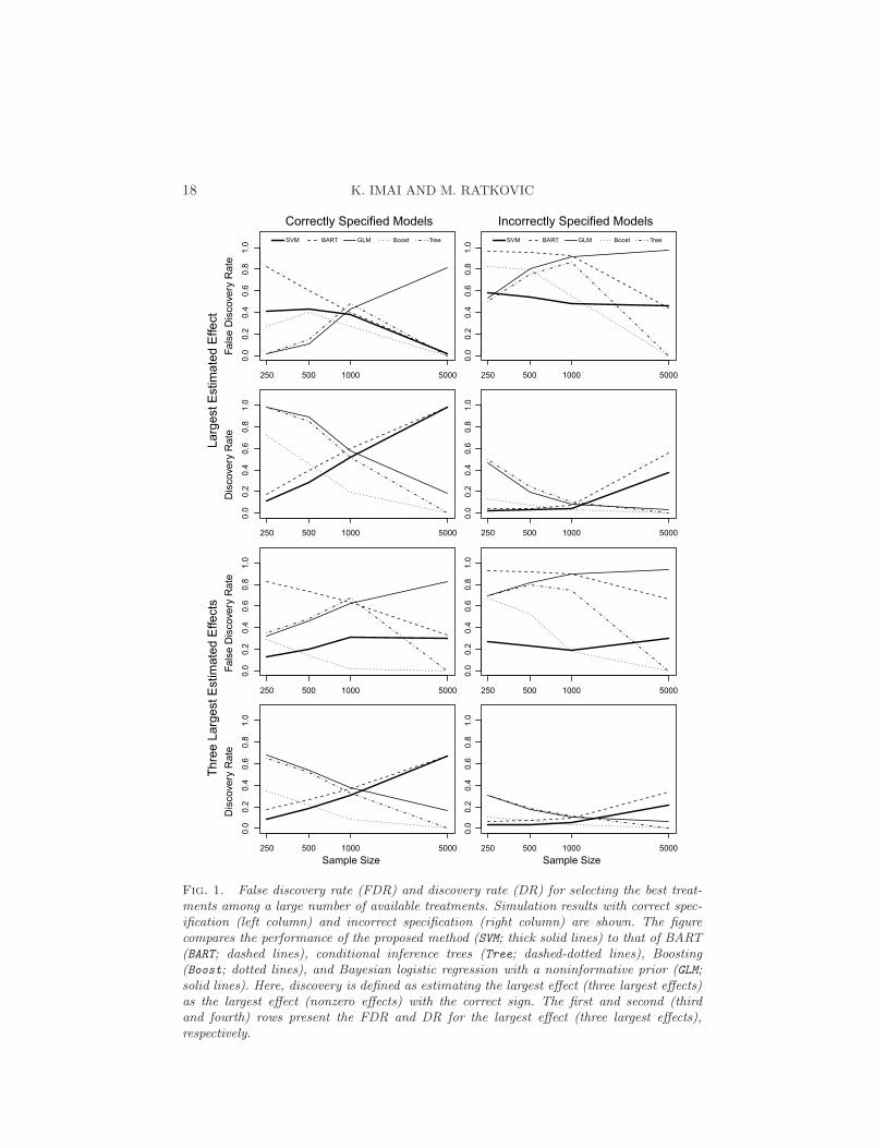
Figure 1 summarizes the results in terms of false discovery rate (FDR)and discovery rate (DR) separately for the largest and substantive effects.We define discovery as estimating the largest effect (three largest effects)as the largest effect (nonzero effects) with the correct sign. Similarly, falsediscovery occurs when the largest effect is not correctly discovered and atleast one coefficient is estimated to be nonzero. FDR may not equal oneminus DR because the former is based only on the simulations where at leastone coefficient is estimated to be nonzero. The first row presents FDR for thelargest effect whereas the second row presents its DR. Similarly, the thirdrow plots the FDR for the three largest effects while the fourth row presentstheir DR. Note that fewer than three nonzero effects may be estimated.

The results show that across simulations the proposed method (SVM; solidlines) has a smaller FDR while its DR is competitive with other methods.The comparison with BART reveals a key feature of our method. The pro-posed method dominates BART in FDR regardless of model specification.The largest estimated effect from BART identifies the largest effect slightlymore frequently, but at the cost of a higher FDR. Despite its low FDR, ourmethod maintains a competitive DR. For many methods, model misspecifi-cation increases FDR and reduces DR. For this reason, we recommend erringin favor of including too many rather than too few pre-treatment covariatesin the model.

Unlike three of its competitors, Boosting, conditional inference trees, andBayesian GLM, the performance of the proposed method improves as thesample size increases. Boosting and trees both attain an FDR and DR of


Fig. 1. False discovery rate (FDR) and discovery rate (DR) for selecting the best treat-ments among a large number of available treatments. Simulation results with correct spec-ification (left column) and incorrect specification (right column) are shown. The figurecompares the performance of the proposed method (SVM; thick solid lines) to that of BART(BART; dashed lines), conditional inference trees (Tree; dashed-dotted lines), Boosting(Boost; dotted lines), and Bayesian logistic regression with a noninformative prior (GLM;solid lines). Here, discovery is defined as estimating the largest effect (three largest effects)as the largest effect (nonzero effects) with the correct sign. The first and second (thirdand fourth) rows present the FDR and DR for the largest effect (three largest effects),respectively.


zero as the sample size grows. The tree focuses in on the largest effects, notidentifying any small effects as the sample size grows. This may be due tothe fact that trees do not converge asymptotically to the true conditionalmean function unless the underlying function is piecewise constant (thoughthey converge to the minimal risk) [see, e.g., Breiman et al. (1984)]. Theboosting algorithm uses trees as base learners, which may be leading to thedeteriorating performance in identifying small effects. The performance ofBayesian GLM also declines with increasing sample size, because we arenot considering uncertainty in the posterior mean estimates. To address thisissue, one must use some p-value based regularization, such as using a p-valuethreshold of 0.10 (see Figure 2 in the next set of simulations for illustration).

4.2. Identifying units for which a treatment is beneficial/harmful. In thesecond set of simulations, we consider the problem of identifying groups ofunits for which a treatment is beneficial (or harmful). Here, we are interestedin identifying interactions between a treatment and observed pre-treatmentcovariates. The key difference between this simulation and the previous one isthat in the current setup causal heterogeneity variables (treatment-covariateinteractions) may be correlated with each other as well as other noncausalvariables. The previous simulation setting assumes that causal heterogeneityvariables (treatment indicators) are independent of each other and othervariables. In this simulation, we also include a comparison with the logisticregression with a single LASSO constraint and the maximal ten-fold cross-validation on the “value” statistic [Qian and Murphy (2011)]. This statisticis the expected benefit from a particular treatment rule [see also Imai andStrauss (2011)]. Note that in the previous simulation, due to a large numberof treatments, cross-validation on this statistic is not feasible.

In the current simulation, we have a single treatment condition, that is,K = 1, and 20 pre-treatment covariates Xi. The pre-treatment covariatesare all based on the multivariate normal distribution with mean zero and arandom variance-covariance matrix as in the previous simulation study, withfive covariates then discretized using 0.5 as a threshold. Causal heterogeneityvariables Zi consist of 20 treatment-covariate interactions plus the maineffect for the treatment indicator (LZ = 21), while Vi is composed of themain effects for the pre-treatment covariates (LV = 20).

Given this setup, we generate the outcome variable Yi in the same wayas in Section 4.1 according to the linear probability model. There are 4pre-treatment covariates that interact with the treatment in a systematicmanner. As before, we apply an affine transformation so that an observationwhose values for these two covariates are one standard deviation above themean has the CATE of roughly 4 and 1.7 percentage points. That is, we setβ = {−2.7,2.7,−6.7,−6.7, . . .} and γ = {50,−30,30,20,−20, . . .} where the. . . denotes uniform draws from [−0.7,0.7].


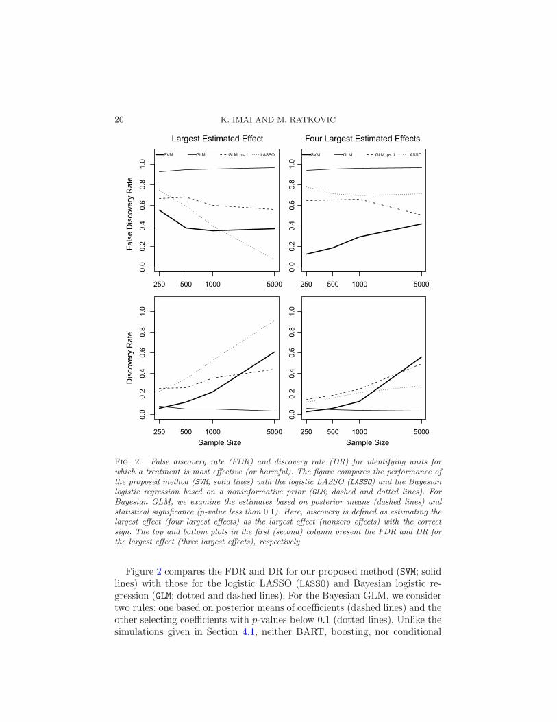
Fig. 2. False discovery rate (FDR) and discovery rate (DR) for identifying units forwhich a treatment is most effective (or harmful). The figure compares the performance ofthe proposed method (SVM; solid lines) with the logistic LASSO (LASSO) and the Bayesianlogistic regression based on a noninformative prior (GLM; dashed and dotted lines). ForBayesian GLM, we examine the estimates based on posterior means (dashed lines) andstatistical significance (p-value less than 0.1). Here, discovery is defined as estimating thelargest effect (four largest effects) as the largest effect (nonzero effects) with the correctsign. The top and bottom plots in the first (second) column present the FDR and DR forthe largest effect (three largest effects), respectively.

Figure 2 compares the FDR and DR for our proposed method (SVM; solidlines) with those for the logistic LASSO (LASSO) and Bayesian logistic re-gression (GLM; dotted and dashed lines). For the Bayesian GLM, we considertwo rules: one based on posterior means of coefficients (dashed lines) and theother selecting coefficients with p-values below 0.1 (dotted lines). Unlike thesimulations given in Section 4.1, neither BART, boosting, nor conditional


inference trees provide a simple rule for variable selection in this setting andhence no results are reported.

The interpretation of these plots is identical to that of the plots in Fig-ure 1. In the left column, the top (bottom) plot presents FDR (DR) for thelargest effect, whereas that of the right column presents FDR (DR) for thefour largest effects. When compared with the Bayesian GLM, the proposedmethod has a lower FDR for both largest and four largest estimated effects.The p-value thresholding improves the Bayesian GLM, and yet the proposedmethod maintains a much lower FDR and comparable DR. Relative to theLASSO, the proposed method is not as effective in considering the largestestimated effect except that it has a lower FDR when the sample size issmall. However, when considering the four largest estimated effects, the pro-posed method maintains a lower FDR than the LASSO, and a comparableDR. This result is consistent with the fact that the value statistic targets thelargest treatment effect while the GCV statistic corresponds to the overall fit.

To further evaluate our method, we consider a situation where each methodis applied to a sample and then used to generate a treatment rule for eachindividual in another sample. For each method, a payoff, characterized bythe net number of people in the new sample who are assigned to treatmentand are in fact helped by the treatment, is calculated. To represent a bud-get constraint faced by most researchers, we specify the total number ofindividuals who can receive the treatment and vary this number within thesimulation study.

Specifically, after fitting each model to an initial sample, we draw anothersimple random sample of 2000 observations from the same data generat-ing process. Using the result from each method, we calculate the predictedCATE for each observation of the new sample, τ(1; Xi), and give the treat-ment to those with highest predicted CATEs until the number of treatedobservations reaches the pre-specified limit. Finally, a payoff of the form1{τ (1; Xi) > 0} · sgn(τ(1;Xi)) is calculated for all treated observations ofthe new sample where τ(1;Xi) is the true CATE. This produces a payoffof 0.5 if a treated observation is actually helped by the treatment, −0.5 ifthe observation is harmed, and 0 for untreated observations. As a baseline,we compare each method to the “oracle” treatment rule, 1{τ(1;Xi) > 0} ·sgn(τ(1;Xi)), which administers the treatment only when helpful. We have

also considered an alternative payoff of the form 1{τ(1; Xi) > 0} · τ(1;Xi),representing how much (rather than whether) the treatment helps or harms.The results were qualitatively similar to those presented here.

The results from the simulation are presented in Table 4. The tablepresents a comparison of payoffs, by method, as a percentage of the op-timal oracle rule, which is considered as 100%. The bottom row presents theoutcome if every observation were treated, indicating that in this simula-tion the average treatment effect is negative but there exists a subgroup forwhich treatment is beneficial. The proposed method (SVM) narrowly domi-


Table 4

Performance in payoff relative to the oracle

Sample size

Method 250 500 1000 5000

SVM −2 11 22 42BART −19 −4 8 21LASSO −18 2 15 28GLM −20 −7 7 34Boost −1 10 18 40Tree 2 2 2 5Treat everyone −123 −121 −121 −116

Note: The table presents a payoff for each method as a percentage of the optimal oraclerule, which is considered as 100%. Each method is fit to a training set, and the treatmentis administered to every person in the validation set with a predicted improvement. Theproposed method (SVM) narrowly dominates Boosting (Boost), and both the proposedmethod and Boosting noticeably outperform all other competitors, except conditionalinference trees (Tree) at sample size 250. At larger sample sizes the tree severely underfits.While the proposed method and Boosting perform similarly by a predictive criterion,Boosting does not return an interpretable model. BART, GLM, and LASSO represent theBayesian Additive Regression Tree, the logistic regression with a noninformative prior,and the logistic regression with a single LASSO constraint and cross-validation on thevalue statistic. The bottom row presents the outcome if every observation were treated,indicating that in this simulation the average treatment effect is negative, but there existsa subgroup for which the treatment is beneficial.

nates Boosting (Boost), and both the proposed method and Boosting no-ticeably outperform all other competitors, except conditional inference trees(Tree) at sample size 250. At larger sample sizes, however, the tree severelyunderfits. While the proposed method and Boosting perform similarly by apredictive criterion, Boosting does not return an interpretable model. Wealso find that SVM outperforms LASSO, which is consistent with the fact thatthe GCV statistic targets the overall performance while the value statisticfocuses on the largest treatment effect. If administering the treatment iscostless, the proposed method generates the most beneficial treatment ruleamong its competitors.

Figure 3 presents the results across methods and sample sizes in the pres-ence of a budget constraint. The left column shows the proportion of treatedunits that actually benefit from the treatment for each observation consid-ered for the treatment in the order of predicted CATE (the horizontal axis).The oracle identifies those who certainly benefit from the treatment andtreats them first. The middle column shows the proportion of treated unitsthat are hurt by the treatment. Here, the oracle never hurts observationsand hence is represented by the horizontal line at zero. The right columnpresents the net benefit by treatment rule, which can be calculated as the


Fig. 3. The relative performance of individualized treatment rules derived by eachmethod. The figure presents the proportion of treated units (based on the treatment rule ofeach method) who benefit from the treatment (left column), are harmed by the treatment(middle column), and the difference between the two (right column) at each percentile ofthe total sample who can be assigned to the treatment. The oracle (solid lines) treats eachobservation only when helpful and hence is identical to the horizontal line at zero in themiddle column. The proposed method (SVM; solid thick lines) makes fewer mistreatmentsthan other methods, while it is conservative in assigning observations to the treatment.


difference between the positive (left column) and negative (middle column)effects. Each row presents a different sample size to which each method isapplied.

The figure shows that when the sample size is small, the proposed methodassigns fewer observations a harmful treatment, relative to its competitors.For moderate and large sample sizes, the proposed method dominates itscompetitors in both identifying a group that would benefit from the treat-ment and avoiding treating those who would be hurt. This can be seenfrom the plots in the middle column where the result based on the pro-posed method (SVM; solid thick lines) stays close to the horizontal zero linewhen compared to other methods. Similarly, in the right column, the resultsbased on the proposed method stay above other methods. When these linesgo below zero, it implies that a majority of treated observations would beharmed by the treatment. The disadvantage of the proposed method is itsconservativeness. This can be seen in the left column where at the begin-ning of the percentile the solid thick line is below its competitors for smallsample sizes. This difference vanishes as the sample size increases, with theproposed method outperforming its competitors. In sum, when used to pre-dict a treatment rule for out-of-sample observations, the proposed methodmakes fewer harmful prescriptions and often yields a larger net benefit thanits competitors.

5. Concluding remarks. Estimation of heterogeneous treatment effectsplays an essential role in scientific research and policy making. In particu-lar, researchers often wish to select the most efficacious treatments from alarge number of possible treatments and to identify individuals who benefitmost (or are harmed) by treatments. Estimation of treatment effect hetero-geneity is also important when generalizing experimental results to a targetpopulation of interest.

The key insight of this paper is to formulate the identification of het-erogeneous treatment effects as a variable selection problem. Within thisframework, we develop a Support Vector Machine with two separate spar-sity constraints, one for a set of treatment effect heterogeneity parametersof interest and the other for observed pre-treatment effect parameters. Thissetup addresses the fact that in many applications, pre-treatment covariatesare much more powerful predictors than treatment variables of interest ortheir interactions with covariates. In addition, unlike the existing techniquessuch as Boosting and BART, the proposed method yields a parsimoniousmodel that is easy to interpret. Our simulation studies show that the pro-posed method has low false discovery rates while maintaining competitivediscovery rates. The simulation study also shows that the use of our GCVstatistic is appropriate when exploring the treatment effect heterogeneityrather than identifying the single optimal treatment rule.


A number of extensions of the method developed in this paper are pos-sible. For example, we can accommodate other types of outcome variablesby considering different loss functions. Instead of the GCV statistic we use,alternative criteria such as AIC or BIC statistics as well as more targetedquantities such as the average treatment effect for the target population canbe employed. While we use LASSO constraints, researchers may prefer al-ternative penalty functions such as the SCAD or adaptive LASSO penalty.Furthermore, although not directly examined in this paper, the proposedmethod can be extended to the situation where the goal is to choose thebest treatment for each individual from multiple alternative treatments. Fi-nally, it is of interest to consider how the proposed method can be appliedto observational data [e.g., see Zhang et al. (2012) who develop a doubly ro-bust estimator for optimal treatment regimes] and longitudinal data settingswhere the derivation of optimal dynamic treatment regimes is a frequent goal[e.g., Murphy (2003), Zhao et al. (2011)]. The development of such meth-ods helps applied researchers avoid the use of ad hoc subgroup analysis andidentify treatment effect heterogeneity in a statistically principled manner.

APPENDIX: ESTIMATED NONZERO COEFFICIENTS FOREMPIRICAL APPLICATIONS

Table 5

Nonzero coefficient estimates for the New Haven get-out-the-vote experiment

Treatment interactions

Visit Phone Mailings Message Coefficient

Yes Any 0–3 Any 1.50

No No 2 Neighborhood 1.25

Yes No 0 Any 1.04

No Close 0 Close 0.84

Any No 3 Any 0.72Yes Any 0 Any 0.59

Any No 3 Civic 0.49

Yes No 0–3 Close 0.15

No Any 2 Any −0.08

Any Any 3 Civic −0.68

Any Civic 0–3 Civic −0.95No No 2 Close −2.09

Any Civic/Blood 0–3 Civic −2.16

No Neighbor 0–3 Neighbor −2.72

No Civic 0–3 Neighbor −3.67

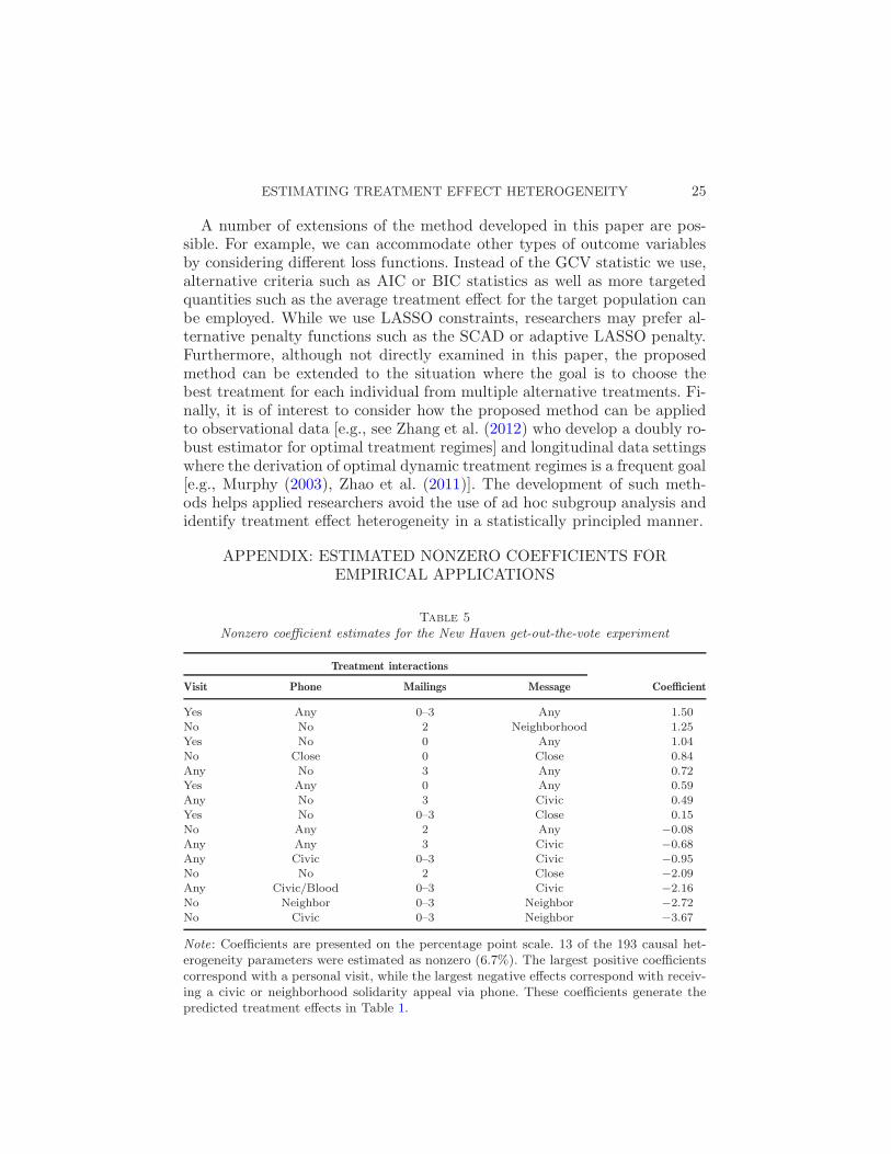
Note: Coefficients are presented on the percentage point scale. 13 of the 193 causal het-erogeneity parameters were estimated as nonzero (6.7%). The largest positive coefficientscorrespond with a personal visit, while the largest negative effects correspond with receiv-ing a civic or neighborhood solidarity appeal via phone. These coefficients generate thepredicted treatment effects in Table 1.


Table 6

Nonzero coefficient estimates for the job training program data

NSW PSID

Treatment intercept 6.92 6.67Main effects

Age 0.00 −0.83Married 1.32 3.39White 0.00 0.10

Squared termsAge2 −0.03 −0.09Education2 0.89 0.86

Interaction termsNo HS degree, Unemployed in 1975 −1.06 0.00White, Married 0.00 26.16White, No HS degree 25.35 30.65Hispanic, Logged 1975 earnings −49.36 −62.15Black, Logged 1975 earnings 8.29 0.00White, Education 0.00 −1.41Married, Education 4.90 12.11Married, Logged 1975 earnings 0.00 5.72Education, Unemployed in 1975 7.52 9.59Age, Education 0.00 −0.47Age, Black −0.56 0.00Age, Hispanic 0.00 0.34Age, Unemployed in 1975 3.30 4.79

Note: The table presents the estimates from the model fitted to the NSW Data without(left column) and with the PSID weights (right column). Coefficients are rescaled to thepercentage point scale. The first row contains the estimated intercept, which correspondsto the estimated CATE for an observation with characteristics set at the mean of allpre-treatment covariates.

Acknolwedgments. An earlier version of this paper was circulated un-der the title of “Identifying Treatment Effect Heterogeneity through Opti-mal Classification and Variable Selection” and received the Tom Ten HaveMemorial Award at the 2011 Atlantic Causal Inference Conference. Wethank Charles Elkan, Jake Bowers, Kentaro Fukumoto, Holger Kern, MichaelRosenbaum, and Sherry Zaks for useful comments. The Editor, AssociateEditor, and two anonymous reviewers provided useful advice.

REFERENCES

Bradley, P. and Mangasarian, O. L. (1998). Feature selection via concave minimiza-tion and support vector machines. In Machine Learning Proceedings of the FifteenthInternational Conference 82–90. Morgan Kaufmann, San Francisco, CA.

Breiman, L., Friedman, J. H., Olshen, R. A. and Stone, C. J. (1984). Classifica-tion and Regression Trees. Wadsworth Advanced Books and Software, Belmont, CA.MR0726392

http://www.ams.org/mathscinet-getitem?mr=0726392


Cai, T., Tian, L., Wong, P. H. and Wei, L. J. (2011). Analysis of randomized compar-ative clinical trial data for personalized treatment selections. Biostatistics 12 270–282.

Chipman, H. A., George, E. I. and McCulloch, R. E. (2010). Bart: Bayesian additiveregression trees. Ann. Appl. Stat. 4 266–298. MR2758172

Cole, S. R. and Stuart, E. A. (2010). Generalizing evidence from randomized clinicaltrials to target populations: The ACTG 320 trial. Am. J. Epidemiol. 172 107–115.

Crump, R. K., Hotz, V. J., Imbens, G. W. and Mitnik, O. A. (2008). Nonparametrictests for treatment effect heterogeneity. The Review of Economics and Statistics 90389–405.

Davison, A. C. (1992). Treatment effect heterogeneity in paired data. Biometrika 79463–474.

Dehejia, R. H. and Wahba, S. (1999). Causal effects in nonexperimental studies: Reeval-uating the evaluation of training programs. J. Amer. Statist. Assoc. 94 1053–1062.

Efron, B.,Hastie, T., Johnstone, I. andTibshirani, R. (2004). Least angle regression.Ann. Statist. 32 407–499. MR2060166

Franc, V., Zien, A. and Scholkopf, B. (2011). Support vector machines as probabilisticmodels. In The 28th International Conference on Machine Learning 665–672. ACM,Bellevue, WA.

Frangakis, C. (2009). The calibration of treatment effects from clinical trials to targetpopulations. Clin. Trials 6 136–140.

Freund, Y. and Schapire, R. E. (1999). A short introduction to boosting. In Proceedingsof the Sixteenth International Joint Conference on Artificial Intelligence 1401–1406.Morgan Kaufmann, San Francisco, CA.

Friedman, J. H., Hastie, T. and Tibshirani, R. (2010). Regularization paths for gen-eralized linear models via coordinate descent. Journal of Statistical Software 33 1–22.

Gail, M. and Simon, R. (1985). Testing for qualitative interactions between treatmenteffects and patient subsets. Biometrics 41 361–372.

Gelman, A., Jakulin, A., Pittau, M. G. and Su, Y.-S. (2008). A weakly informativedefault prior distribution for logistic and other regression models. Ann. Appl. Stat. 21360–1383. MR2655663

Gerber, A. S. and Green, D. P. (2000). The effects of canvassing, telephone calls, anddirect mail on voter turnout: A field experiment. American Political Science Review 94653–663.

Gerber, A., Green, D. and Larimer, C. (2008). Social pressure and voter turnout:Evidence from a large-scale field experiment. American Political Science Review 10233–48.

Green, D. P. and Kern, H. L. (2010a). Detecting heterogenous treatment effects inlarge-scale experiments using Bayesian additive regression trees. In The Annual SummerMeeting of the Society of Political Methodology. Univ. Iowa.

Green, D. P. andKern, H. L. (2010b). Generalizing experimental results. In The AnnualMeeting of the American Political Science Association. Washington, D.C.

Gunter, L., Zhu, J. and Murphy, S. A. (2011). Variable selection for qualitative inter-actions. Stat. Methodol. 8 42–55. MR2741508

Hartman, E., Grieve, R. and Sekhon, J. S. (2010). From SATE to PATT: The essentialrole of placebo test combining experimental and observational studies. In The AnnualMeeting of the American Political Science Association. Washington, D.C.

Hill, J. L. (2011). Challenges with propensity score matching in a high-dimensionalsetting and a potential alternative. Multivariate and Behavioral Research 46 477–513.

Hothorn, T., Hornik, K. and Zeileis, A. (2006). Unbiased recursive partitioning:A conditional inference framework. J. Comput. Graph. Statist. 15 651–674. MR2291267







Imai, K. (2005). Do get-out-the-vote calls reduce turnout?: The importance of statisticalmethods for field experiments. American Political Science Review 99 283–300.

Imai, K. and Strauss, A. (2011). Estimation of heterogeneous treatment effects fromrandomized experiments, with application to the optimal planning of the get-out-the-vote campaign. Political Analysis 19 1–19.

Kang, J., Su, X., Hitsman, B., Liu, K. and Lloyd-Jones, D. (2012). Tree-structuredanalysis of treatment effects with large observational data. J. Appl. Stat. 39 513–529.MR2880431

Lagakos, S. W. (2006). The challenge of subgroup analyses–reporting without distorting.N. Engl. J. Med. 354 1667–1669.

LaLonde, R. J. (1986). Evaluating the econometric evaluations of training programs withexperimental data. American Economic Review 76 604–620.

LeBlanc, M. and Kooperberg, C. (2010). Boosting predictions of treatment success.Proc. Natl. Acad. Sci. USA 107 13559–13560.

Lee, Y., Lin, Y. and Wahba, G. (2004). Multicategory support vector machines: Theoryand application to the classification of microarray data and satellite radiance data.J. Amer. Statist. Assoc. 99 67–81. MR2054287

Lin, Y. (2002). Support vector machines and the Bayes rule in classification. Data Min.Knowl. Discov. 6 259–275. MR1917926

Lipkovich, I., Dmitrienko, A., Denne, J. and Enas, G. (2011). Subgroup identificationbased on differential effect search—a recursive partitioning method for establishingresponse to treatment in patient subpopulations. Stat. Med. 30 2601–2621. MR2815438

Loh, W. Y., Piper, M. E., Schlam, T. R., Fiore, M. C., Smith, S. S., Jorenby, D. E.,Cook, J. W., Bolt, D. M. and Baker, T. B. (2012). Should all smokers use com-bination smoking cessation pharmacotherapy? Using novel analytic methods to detectdifferential treatment effects over eight weeks of pharmacotherapy. Nicotine and TobaccoResearch 14 131–141.

Manski, C. F. (2004). Statistical treatment rules for heterogeneous populations. Econo-metrica 72 1221–1246. MR2064712

Menon, A. K., Jiang, X., Vembu, S., Elkan, C. and Ohno-Machado, L. (2012).Predicting accurate probabilities with a ranking loss. In Proceedings of the 29th Inter-national Conference on Machine Learning. Edinburgh, Scotland.

Moodie, E. E. M., Platt, R. W. and Kramer, M. S. (2009). Estimating response-maximized decision rules with applications to breastfeeding. J. Amer. Statist. Assoc.104 155–165. MR2663039

Murphy, S. A. (2003). Optimal dynamic treatment regimes. J. R. Stat. Soc. Ser. B Stat.Methodol. 65 331–366. MR1983752

Nickerson, D. W. (2008). Is voting contagious?: Evidence from two field experiments.American Political Science Review 102 49–57.

Pineau, J., Bellemare, M. G., Rush, A. J., Ghizaru, A. and Murphy, S. A. (2007).Constructing evidence-based treatment strategies using methods from computer sci-ence. Drug and Alcohol Dependence 88S S52–S60.

Platt, J. (1999). Probabilistic outputs for support vector machines and comparison toregularized likelihood methods. In Advances in Large Margin Classifiers 61–74. MITPress, Cambridge, MA.

Qian, M. and Murphy, S. A. (2011). Performance guarantees for individualized treat-ment rules. Ann. Statist. 39 1180–1210. MR2816351

Ratkovic, M. and Imai, K. (2012). FindIt: R package for finding heterogeneous treatmenteffects. Available at Comprehensive R Archive Network (http://cran.r-project.org/package=FindIt).












Rosenbaum, P. R. and Rubin, D. B. (1983). The central role of the propensity score inobservational studies for causal effects. Biometrika 70 41–55. MR0742974

Rothwell, P. M. (2005). Subgroup analysis in randomized controlled trials: Importance,indications, and interpretation. The Lancet 365 176–186.

Rubin, D. B. (1990). Comment on J. Neyman and causal inference in experiments andobservational studies: “On the application of probability theory to agricultural exper-iments. Essay on principles. Section 9” [Ann. Agric. Sci. 10 (1923) 1–51]. Statist. Sci.5 472–480. MR1092987

Sollich, P. (2002). Bayesian methods for support vector machines: Evidence and predic-tive class probabilities. Machine Learning 46 21–52.

Stuart, E. A., Cole, S. R., Bradshaw, C. P. and Leaf, P. J. (2011). The use ofpropensity scores to assess the generalizability of results from randomized trials. J. Roy.Statist. Soc. Ser. A 174 369–386. MR2898850

Su, X., Tsai, C. L., Wang, H., Nickerson, D. M. and Li, B. (2009). Subgroup analysisvia recursive partitioning. J. Mach. Learn. Res. 10 141–158.

Tibshirani, R. (1996). Regression shrinkage and selection via the lasso. J. Roy. Statist.Soc. Ser. B 58 267–288. MR1379242

Vapnik, V. N. (1995). The Nature of Statistical Learning Theory. Springer, New York.MR1367965

Wahba, G. (1990). Spline Models for Observational Data. CBMS-NSF Regional Confer-ence Series in Applied Mathematics 59. SIAM, Philadelphia, PA. MR1045442

Wahba, G. (2002). Soft and hard classification by reproducing kernel Hilbert space meth-ods. Proc. Natl. Acad. Sci. USA 99 16524–16530 (electronic). MR1947755

Yang, Y. and Zou, H. (2012). An efficient algorithm for computing the HHSVM and itsgeneralizations. J. Comput. Graph. Statist. To appear.

Yuan, M. and Lin, Y. (2006). Model selection and estimation in regression with groupedvariables. J. R. Stat. Soc. Ser. B Stat. Methodol. 68 49–67. MR2212574

Zhang, T. (2004). Statistical behavior and consistency of classification methods based onconvex risk minimization. Ann. Statist. 32 56–85. MR2051001

Zhang, H. H. (2006). Variable selection for support vector machines via smoothing splineANOVA. Statist. Sinica 16 659–674. MR2267254

Zhang, B., Tsiatis, A. A., Laber, E. B. and Davidian, M. (2012). A robust methodfor estimating optimal treatment regimes. Biometrics. To appear.

Zhao, Y., Zeng, D., Socinski, M. A. and Kosorok, M. R. (2011). Reinforcementlearning strategies for clinical trials in nonsmall cell lung cancer. Biometrics 67 1422–1433. MR2872393

Zhao, Y., Zeng, D., Rush, J. A. and Kosorok, M. R. (2012). Estimating individualizedtreatment rules using outcome weighted learning. J. Amer. Statist. Assoc. 107 1106–1118.

Zou, H. and Hastie, T. (2005). Regularization and variable selection via the elastic net.J. R. Stat. Soc. Ser. B Stat. Methodol. 67 301–320. MR2137327

Zou, H., Hastie, T. and Tibshirani, R. (2007). On the “degrees of freedom” of thelasso. Ann. Statist. 35 2173–2192. MR2363967

Department of Politics

Princeton University

Princeton, New Jersey 08544

USA

E-mail: [email protected]@princeton.edu

URL: http://imai.princeton.edu














mailto:[email protected]

mailto:[email protected]

http://imai.princeton.edu

Documents

Estimating treatment effect heterogeneity in randomized ... · 2 K. IMAI AND M. RATKOVIC heterogeneity as the degree to which different treatments have differential causal effects